Submitted:
27 June 2024
Posted:
27 June 2024
You are already at the latest version
Abstract
The development of virtual models has recently been generalized in the field of complex mechatronic product design. Virtual models have various advantages such as: the systemic design approach, most often parametric, the implementation of extreme, expensive, and perhaps risky scenarios for the operation of the designed product, the testing of a large number of variants, etc.
The main contribution of the paper consists of the development of an interface family called DeSeRoI (Dedicated Serial Robot Interface). Each member of the interface family integrates Simulink libraries and is created by the programmer in accordance with user requests. It follows that the interfaces composing the DeSeRoI family can have different levels of complexity depending on user needs and constraints.
We are implementing a MATLAB-based application with user-provided configuration for serial robots in order to automatically visualize the kinematics data and simulation. Within MATLAB, two scripts are created responsible for generating Simulink models that compute the kinematics problem. One of the scripts (Main) saves information about the configuration of the robot and the other one (Generates_Simulink_Models) computes the kinematics problem. Different types of functions (software module) have been developed. Using these functions, the Simulink models result as modular entities. The automated approach eases user’s interaction and understanding of serial robots’ kinematics by performing the simulation procedure in a shorter amount of time and with higher efficiency, assuring a precise outcome despite the chosen parameters.
Keywords:
serial robots
; kinematics
; simulation model
; interchangeable configuration
; virtual models
1. Introduction
In the field of manufacturing, there is an ongoing quest for efficiency, flexibility and productivity, which is shaping industry practices and driving innovation and competitiveness. With the intention of achieving all of the above, manufacturers and engineers are implementing innovative technologies and methodologies to enhance productivity in their operations. These technologies and methods that are currently employed include automation [1], collaborative robots [2], lean manufacturing [3], additive manufacturing (3D printing) [4], IoT [5], and simulation [6] among others.
Each of them have a different benefit and contribute to innovation in their unique way. Automation and collaborative robotics contribute to the enhancement of efficiency [7,8], additive manufacturing and collaborative robots improve the flexibility [9,10], IoT and lean manufacturing contribute to sustainability and cost reduction, and IoT, additive manufacturing and simulation boost the productivity [11].
In addition to these widely adopted methods, the manufacturing industry regularly employs serial robots (SR). They perform various operations such as assembling components, welding, quality control, machining, and handling materials. To ensure the functionality and seamless integration of SR into systems, several steps must be followed, including: design, simulation, hardware and software integration, staff training, monitoring, and maintenance.
Simulation refers to the process of designing and modelling a real or hypothetical physical system, running the model (replicating the real-world use of the physical system in a dynamic virtual environment), and then analyzing the results with respect to a predetermined set of goals that the system has to meet. It is considered a very important tool not only in robotics but in numerous other fields, due to its many positives [18]. A great benefit of using simulation models is the capacity to optimize production processes by introducing a virtual (and thus more cost-effective) feedback loop meant to find errors and oversights made in previous development steps.
It can be observed that simulation is a very common activity in recent years, used across many sciences and disciplines to highlight aspects or demonstrate hypotheses. Concrete uses of simulation include product design, process optimization, medical training, traffic flow analysis, and flight simulators, among others. In the manufacturing industry, simulation is essential for the optimization of processes and refining of the product design. In robotics, simulation plays an important role in development and testing, ensuring that they are efficient and safe.
Scientists from various fields presented the importance of simulation in education [12], manufacturing [13], nursing education [14], robotics [15,16,17], and many others. Hereafter, simulation will be discussed, with a focus on the simulation of serial robots.
To ensure optimal performance, SR are extensively simulated for various behaviors. These simulations include path planning for optimal routing, task execution for jobs like assembly or welding, and kinematics and dynamics to validate motion and forces. They can also cover error handling, force control, and sensor integration. Such comprehensive simulations validate that SR are accurate and safe to use in industrial operations [19,20,21].
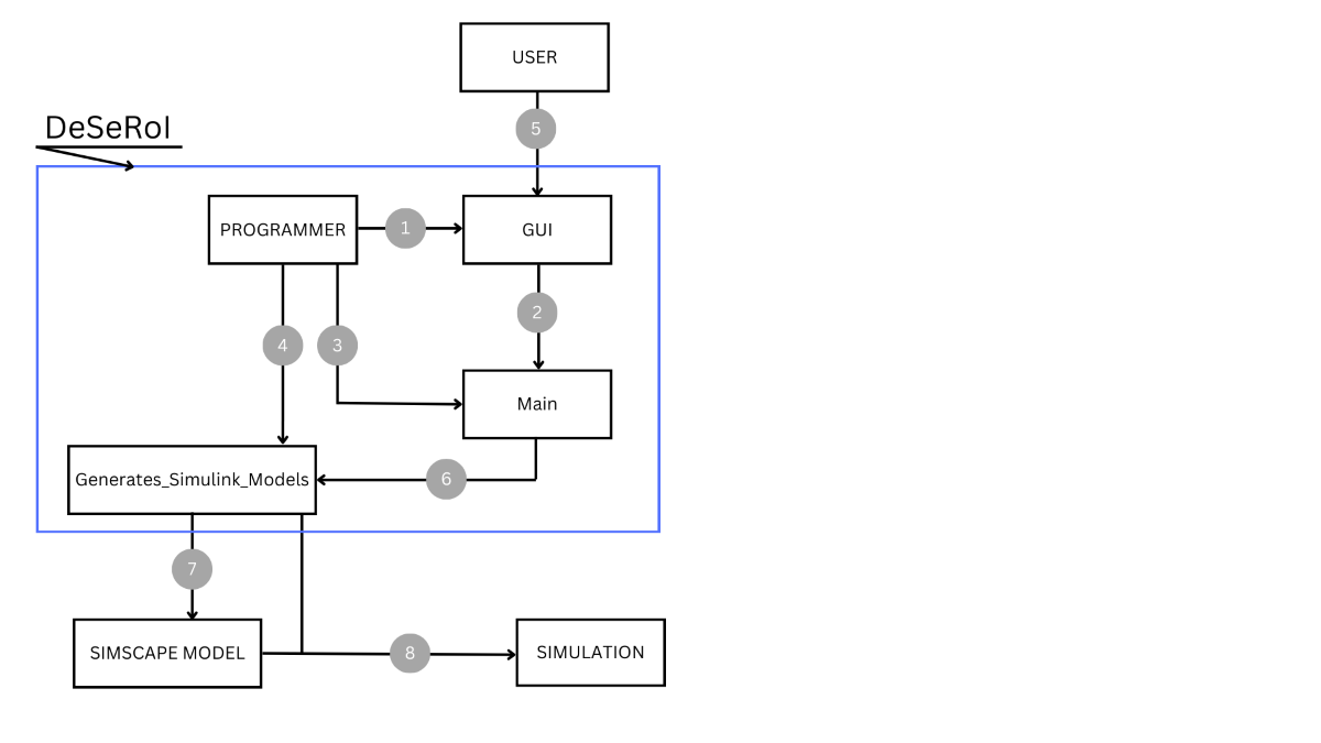
The main contribution of the paper consists of the development of an interface family called DeSeRoI (Dedicated Serial Robot Interface) (Figure 1). Each member of the interface integrates Simulink libraries and is created by the programmer in accordance with user requests. It follows that the interfaces composing the DeSeRoI family can have different levels of complexity depending on user needs and constraints. DeSeRoI is characterized by the following:
- a)
- Adaptability to constraints imposed by the user. Therefore, being able to have various complexity levels implemented by the programmer.
- b)
- It is necessary to preinstall MATLAB but it is not necessary for the user to have MATLAB knowledge
- c)
- Depending on its complexity, any serial robot configuration can be simulated.
Figure 1.
DeSeRoI general template.
The rest of the paper is organized as follows: Section 2, applications used for simulation, Section 3, the structure of the proposed application is presented and all of the component parts are described in detail. In Section 4, an example is provided for validation reasons and to emphasize the importance of the application.
2. Related Work
Building on the presented concepts, researchers have conducted significant work to enhance the capabilities and applications of serial robots. Nam et al. propose a vehicle crash simulator [22] that, unlike most simulators, which focus on a single vehicle, simulates both vehicles and their environments. Their simulator integrates Simpy-based vehicle collision simulations with Unity-based animation for comprehensive visualization of crash scenarios. Vehicle and environment models are previously stored. The model adjusts the characteristics of the vehicle model according to the discrete events sent by the Simpy engine and identifies the collisions that might occur on the road. However, there are some potential limitations that could arise, for instance, the simulator’s dependence on the model repository means that any inaccuracies in the stored models could lead to unreliable simulation outcomes. Additionally, the reliance on JSON files for communication between the simulation and animation components introduces potential transmission issues, which could lead to incorrect animations.
Another utility of simulation is that it can assist in the practical implementation of swarm robotics, enclosing the gap between concept and real-world application. Different multi-robot simulators were developed for simulation of swarm robotics as presented in [23]. Each of them has specific characteristics depending on the aspects to be simulated such as the capability to simulate multiple mobile robots (Stage), high-level modeling language for analyzing the swarm robotics systems (Bio-PEPA), built-in collision detection system (Open Dynamics Engine), the generation of consistent interaction between objects (Gazebo). Additionally, a simulation using OOP (Object-Oriented Programming) is presented in [24].
A simulation model was developed by Bencak et al. for the determination of an object’s optimal pick-point due to its complexity [25]. The simulation model is based on ADAMS/MATLAB cosimulation, with the mechanical model created in ADAMS and the force controller, support functions and user interface developed in MATLAB/Simulink, respectively MATLAB/App Designer. The proposed model is capable of simulating a variety of objects and of suggesting new configurations for the existing robotic gripper. The main disadvantage of the model is the reliance on exact values for contact and other parameters, which are challenging to verify without highly accurate sensors. Moreover, the simulation achieves less accuracy than simulations conducted using alternative methods.
Similar computer applications were developed to teach forward and inverse kinematics. Gonzalez-Garcia et al. used an experimental platform based on MATLAB’s Sim-scape Multibody library in order to validate that computer simulations are very effective in teaching robotics to undergraduates [26]. The approach involves creating 3D robot models in Solidworks, converting them to STL and XML files using Simscape Multibody library tools, and importing these files into Matlab/Simulink to create a mechanical model. The virtual model is afterwards configured in three sections. In the input parameters section users adjust the joint positions. The forward kinematics section is where D-H parameters are set, the reference systems are defined, and transformation matrices are calculated. Finally, in the results display section, users can visualize the positions and orientations of each joint. When the model is first loaded, the reference systems are at the robot’s base, so the user must redefine each of them according to the D-H method.
Arnay et al. developed a software suite made of two applications based on Python and Unity3D [27] in which, after a file containing the configuration of the robot is processed, students are presented with a 2D schematic and a 3D model of the robot, achieving comprehensive learning experience. The first application, implemented as a Python script, extracts the configuration of the robot, and generates its visual schematic. A user interface was created using Unity3D in which the students have to define joint reference systems. In contrast, the second application, developed using Unity3D, creates an interactive 3D model of the robot that allows the manipulation of joint movements and facilitates the derivation of D-H parameters.
Another educational simulation tool was developed by Sanguino and Márquez [28]. They created a simulation tool that helps with teaching and learning 3D kinematics workspaces without the need of programming knowledge. The graphical interface allows for the definition of D-H parameters and the geometry of a serial robotic arm with up to 5 DOF.
Currently, there is a lot of simulation software available for robot systems. Among the most utilized platforms for modeling and simulation is MATLAB. Some benefits of using MATLAB include: the possibility of real time simulation, powerful visualization tools for analyzing and interpreting simulation results, and the ability to handle complex simulations.
3. Materials and Methods
All the applications mentioned above require the user to create a simulation model for conducting simulations. However, creating a 3D model or a simulation model in MATLAB, for example, can be very time-consuming.
The goal was to develop an application that can help ease the process of simulating the kinematics problem for a serial robot with a desired configuration. The forward kinematics is very important in robotics, mainly for simulations issues, while the inverse kinematics is used for implementation of real-life applications.
The forward kinematics problem involves determining the absolute position and the orientation of the end-effector (EE) when the joint variables are known, whereas the inverse kinematics implies determining the generalized coordinates necessary to achieve a given EE position.
In an effort to make the simulation process easier for the user, the authors propose a MATLAB based application, using Simulink’s Simscape library for modelling purposes. The application provides the simulation of a robotic manipulator based on information provided by the user. In contrast to the standard method, the proposed approach does not require any prior knowledge of MATLAB Simulink, and moreover, it offers the capability to generate simulation models for multiple configurations.
3.1. Generating a Simulation in MATLAB
The following terms are going to be used in the next sections:
User – refers to the end-user interacting with the system.
Programmer – denotes the individual responsible for writing the code, in this case the author.
GUI – stands for Graphical User Interface and represents the interface between User and the application.
Main – refers to the MATLAB script associated with the GUI.
Generates_Simulink_Models – refers to the MATLAB script that creates the Simulink models for the simulation.
RobotStructure - refers to the Simulink model created using Simscape library that contains the links and joints of the robot.
SimulationModel – refers to the Simulink model that computes the requested problem.
For comparison purposes, Table 1 presents a description of generating a kinematics simulation using each of the methods, standard and proposed.
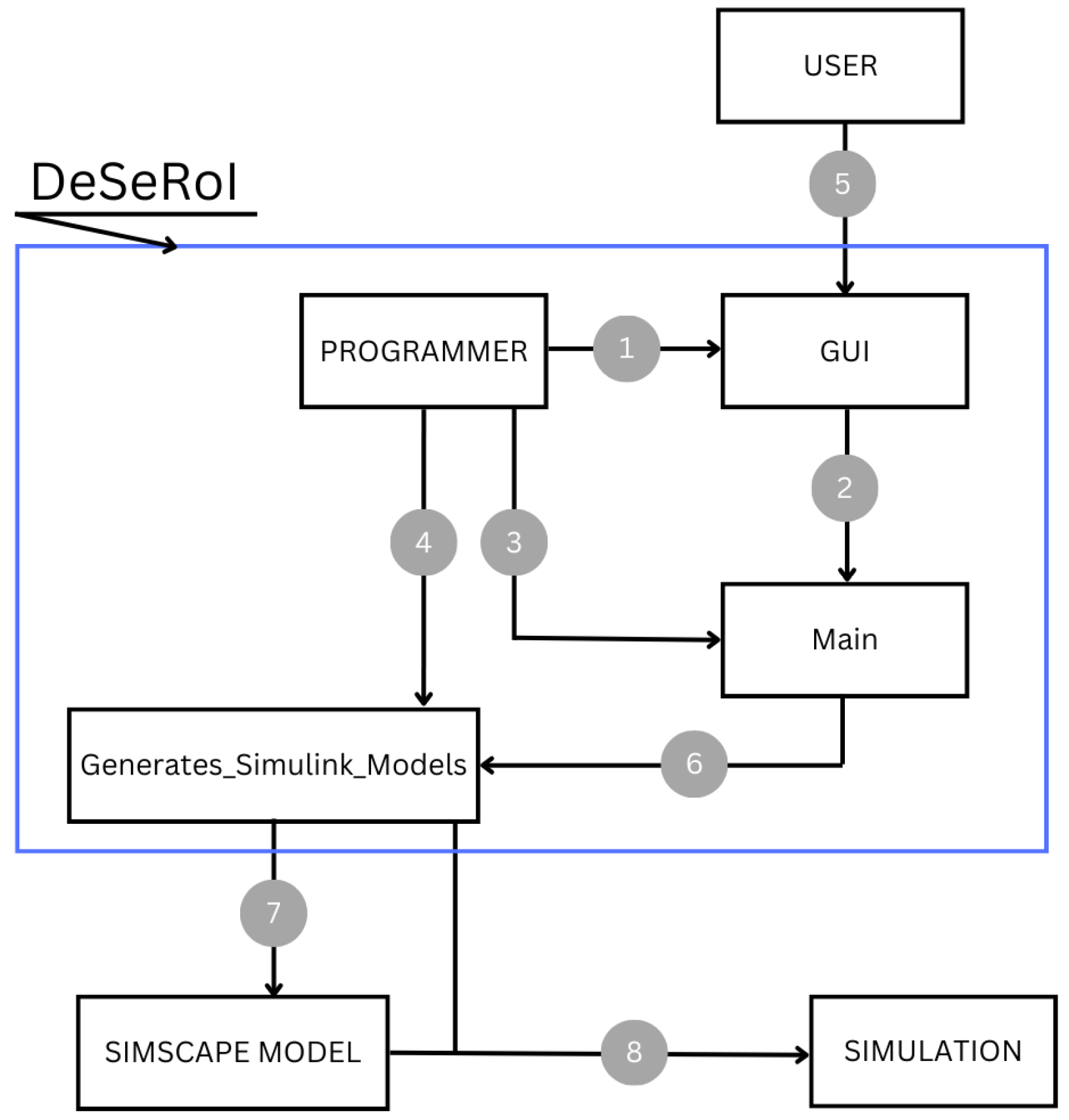
An example of a Simulink model containing the structure of a 3DOF serial robot is provided in Figure 2. 1, 2, 3, and 4 represent the links, while J1, J2, and J3 represent the joints.
In the next paragraph, the process of creating a Simulink model for the structure of a robot will be explained, and some important abbreviations will be clarified so the thought process behind the application can be understood better.
When creating the structure of the robotic arm the user must follow basic Simulink representation rules, for example every movement is around or along the Z axis. The model must contain some mandatory blocks (“Solver Configuration”, “Mechanism Configuration” and “World Frame” - WF) followed by the links and the joints of the robotic arm, and “Rigid Transform” (RT) blocks that make the connection between links and joints. Whenever a link or a joint is added to the model it needs a coordinate system associated to it, that is relative to the previous link or joint. The system, represented by the RT block, is supposed to be in the mass center of the element, and it can be translated and rotated in order to get to a new position. Additionally, if the rotation of a joint is around X axis (in relation to the global reference WF) or the length of a link is along X axis, for example, the RT associated has to be rotated so that its Z axis corresponds to the global reference’s X axis. In Figure 2, RT blocks Z1, Z2, Z3 were added to position links on the right axis, and the other RT blocks WF2Base, Base2Joint1 and so on were added in order to position the following joint or link.
Considering all of the above mentioned, it is obvious that the proposed application is a helpful tool for the user.
3.2. Application Overview
With the purpose of involving the user as little as possible a GUI was created, where the user fills in the data regarding the configuration of the robotic arm and by pressing a button they are provided with the simulation of the desired robot. The overview of the application is presented in Figure 1. The steps that must be followed in the creation of the application are mentioned below and explained in the following subsections.
Step 1: The programmer creates the GUI.
Step 2: The GUI generates its callback script (Main).
Step 3: The programmer makes changes or adds code to Main.
Step 4: The programmer writes the Generates_Simulink_Models script that creates the robot’s Simulink model.
Step 5: The user introduces the information needed for the simulation.
Step 6: Information entered by the user is assigned to specific variables found in Main script.
Step 7: Generates_Simulink_Models generates the Simulink model of the robotic arm.
Step 8: The simulation is provided to the user.
DeSeRoI offers configurable complexity levels customized to user requirements. The application is capable of performing a range of computations, including forward kinematics, inverse kinematics, dynamics problems, and additional functionalities, each of these computations being a member of the DeSeRoI family. This flexibility ensures that varying levels of computational demands and user expertise can be met by the application.
3.3. Graphical User Interface
A GUI is a digital interface in which a user can operate graphical components such as menus, buttons, and text inputs. Through a GUI the user can interact with electronic devices or computer systems. GUIs are used in various types of applications such as software for smartphones, video games, and industrial applications, all because of the intuitiveness and ease that they offer in controlling systems.
The interface was created interactively using a drag-and-drop environment [32]. To open the environment, type “guide” in the Command Window. On the left side of the Editor can be found a menu that contains all the components that can be added as shown in Figure 3.
In order to place the components, they have to be dragged and dropped. The size of the interface can be adjusted by dragging the right bottom corner. After that, by double clicking a component, an Inspector opens where all parameters can be modified. Figure 4 shows the parameter list for a Push Button and an Edit Text.
For the components used, parameters “String” and “FontSize” were changed to match the characteristics of the robotic arm. The “Tag” parameter value is the value that is used in the callback functions in order to identify the component that one is working with. After configuring the parameters, the final design of the interface can be seen in Figure 5. The information required in the GUI refers to the name of the robot, type of the joints, link sizes and joint variables.
The components are going to be reffered to as boxes preceded by their name. The proposed GUI has a total of 35 boxes.
With the aim of creating an intuitive and user-friendly GUI, various types of boxes available were used. For example, to enhance usability and clarity a significant number of “Static Text” boxes were incorporated, which provide explanations for user input fields. For efficient selection of joint types, “Pop-up Menu” boxes were employed, while “Edit” boxes were used for filling-in sizes of the links, values for joint variables, and the name of the robot. Additionally, a “Push button” box responsible for running the simulation was included to streamline the user’s navigation through the process.
Once saved, a MATLAB Script (Main), containing the callback functions is generated based on the actions that took place in the GUI editor. The script has the same name as the figure and is saved in the same folder.
3.4. MATLAB Scripts
The application contains two scripts: Main – the script containing the GUI callbacks and Generates_Simulink_Models – the script that creates the Simulink model for the simulation.
3.4.1. Main Script
Main is the script containing the GUI callbacks that are generated with the creation of the GUI. The script is structured as follows: first, there are the functions that deal with the setup and initialization of the GUI and that manage the GUI’s state and output (Main, Main_OpeningFcn and Main_OutputFcn). Following those, there is a function associated with each box in the interface adding up to a total of 40 functions. Some of the functions in Main are “edit3”, “popupmenu1”, and “pushbutton1”.
For every box in the GUI that is going to contain a value or some information necessary for the simulation model, a variable is created in their respective callback function from Main, responsible with storing the value. As an example, Figure 6 represents the callback function edit3, associated to the “Edit Text” box where the user fills in the name of the robot. The command that stores the value is highlighted in a rectangle.
The functions for the other boxes are similar to the one shown above, except for the “Push Button” function that is responsible for running the Generates_Simulink_Models Script. The function is shown in Figure 7.
The variables are declared as global, each in their own callback function but also in the callback function of the “Push Button” so they can be used in Generates_Simulink_Models. Once run, Main saves all of the data provided by User in GUI and runs Generates_Simulink_Models.
3.4.2. Generates_Simulink_Models Script
The main objective of Generates_Simulink_Models Script is to create the Simulink model of the robotic arm and run its simulation.
The Generates_Simulink_Models Script is structured as shown in Figure 8.
First, the Simulink model containing the configuration of the robot (RobotStructure) was created and saved in order to obtain the Rigid Body Tree, then a new Simulink model was created, tasked with conducting the forward kinematics process (SimulationModel). Following that, there is the command for running the simulation of the model and some useful functions created specifically for this application.
The RobotStructure model only contains the configuration of the robot as seen in Figure 2. It was created using the open_system(new_system()) command. After the model is saved, the corresponding Rigid Body Tree is obtained with the help of importrobot() function [33]. SimulationModel is created just like RobotStructure and it is named according to the user’s input in the GUI plus the current date and time. This model contains “Constant” blocks with the values of the joint variables followed by “Gain” blocks that transform the measurement unit from degrees to radians. The configuration of the robot is also represented here so the outputs from the “Gain” blocks are then provided as inputs for the “Revolute Joint” blocks. This is done by using a “Simulink-PS Converter” for each of the joints, that converts the Simulink input signal to a Physical Signal.
Each one of the joints has an output associated with the position by checking the “Position” box under “Sensing” in the Block parameter. The outputs are connected to a “Mux”, through “PS-Simulink Converter” blocks, which is then connected to a “Get Transform” block. The “Get Transform” block has a parameter called “Rigid Body Tree” where the Rigid Body Tree obtained with the help of the GetRBT function is used. Other parameters that have to be configured are “Source Body” and “Target Body” where the last and the first element of the robot need to be selected. The next block is the “Coordinate Transformation Conversion” that has a homogenous transformation as input and converts it to a translation vector.
To configure parameters for the blocks, the “set_param” command is used, and to establish connections between blocks, the “add_line” command is used.
Because before every link or joint in the structure of the robot a RT has to be added and configured in relation to the previous one (as explained in subsection 3.1), there would be many variations of the RT. With the great number of orientations of the coordinate system, there is a great amount of work to generate diverse configurations. One of the proposed features of the application is to reduce the number of possible orientations for the RT down to three, each of them corresponding to a rotation around one of the axes of the global coordinate system as shown in Figure 9.
To be able to only use the three coordinate systems presented above, it is required to add an additional RT after every link or joint. The additional RT is going to reorient the coordinate system to ensure that it consistently maintains alignment with the WF, the global reference frame of the model [31]. To identify the type of Rigid Transform a variable called varSist is defined. For Figure 9 a) varSist = 3, for Figure 9 b) varSist = 2, and for Figure 9 c) varSist = 1. The necessary transformations to reorient the coordinate system to WF orientation are presented in Figure 10.
Figure 11 presents the structure of a 3DOF robot created using the proposed method.
Based on the grouping of elements in Figure 11, three of the functions in Figure 8 were created: a) Convert_to_WF_Orientation - coresponds to all of the blocks that contain “2WF” in their names, b) AddJoint - coresponds to the blocks in rectangles, c) AddLink - coresponds to the blocks in capsules.
Convert_to_WF_Orientation is the function that adds an intermediate RT block that converts the orientation back to WF orientation as explained previously. The function is called using the name of the last added link or joint, it checks its orientation, transforms it accordingly, and resets varSist to 3, the value specific to WF orientation. The function is presented in Figure 12.
Functions AddJoint and AddLink were created in order to be able to add joints and links in an easier manner. As seen in Figure 12, each joint and link is preceded by an associated RT, with parameters set according to the specific element.
AddJoint = RT block + Joint block
The function adds the RT block, checks for the type of joint, sets the parameters and resets varSist accordingly, then adds the joint block, sets its parameters and makes the connections between blocks. Its input parametres are: 1. SimName – the name of the model that the blocks are added to, 2. C – the variable that saves the joint type selected, 3. numeCupla – the name of the joint block in the model, 4. elemAnterior – the name of the previous link block, 5. cuplaUrmatoare – the abbreviated name of the joint, 6. lx – the length of the previous link on X axis, 7. ly - the length of the previous link on Y axis, 8. lz - the length of the previous link on Z axis.
AddLink = RT block + Link block
AddLink function adds both the RT and the link block, verifies on which axis the link’s length is on, sets the parameters, and makes the connections between the blocks. The input parameters for this function are: 1. SimName – the name of the model that the blocks are added to, 2. numeElem – the name of the link block in the model, 3. cuplaAnterioara – the name of the previous joint block, 4. elemUrmator – the abbreviated name of the link, 5. lx – link length on X axis, 6. ly – link length on Y axis, 7. lz – link length on z axis.
The last function defined in Generates_Simulink_Models is Obtain_Rigid_Body-Tree function containing the importrobot command for obtaining the rigid body tree from RobotStructure model.
4. Validation and Results
To ensure the functionality and effectiveness of the proposed application, a comprehensive validation process was conducted. The validation process is conducted through the following approaches:
- Accuracy verification: The objective is to demonstrate that the simulations generated using the proposed method are equivalent to those obtained using standard theoretical methods (D-H or direction cosines). The coordinate matrix of the origin of system T3 (fourth column in matrix H1, respectively H2) complies with the geometrical values, therefore validating the calculations performed.
- Efficiency analysis: The number of operations performed by the user to complete simulations, was considered as a factor that characterizes efficiency.. The steps involved in both the standard method and the proposed application will be enumerated, demonstrating a significant reduction in user operations with the application.
The application was tested on a system with the following specifications:
- Operating system: Windows 11
- Processor Intel Core i5
- RAM: 8GB
- MATLAB Version: MATLAB R2023a
In the following, a simplified version of DeSeRoI is considered, namely DeSeRoI_Forward_Kinematics (Figure 13), the member of DeSeRoI family that computes the forward kinematics problem. To reduce complexity while maintaining relevancy, it was decided to use a serial robot with 3DOF with only revolute joints. The validation of the developed application was conducted by performing a series of simulations with various configurations of serial robots. The application was configured to perform simulations based on user – defined inputs, being able to handle various input parameters such as: joint types, joint angles, link sizes.
4.1. Accuracy Verification
To validate the accuracy of the application, two serial robots with different configurations were simulated and an H matrix was provided for each of them. The matrix describes the absolute orientation of Link3 and the absolute position of the origin of the coordinate system T3, fixed to Link3 and positioned at the center of Joint3.
The first example is a 3DOF serial robot with the configuration RzRyRz (Figure 14). Its input data can be found in Figure 15.
The simulated position, based on the values in Figure 15, is presented in Figure 16 alongside the H1 matrix mentioned at the beginning of the subsection.
4.2. Efficiency Analysis
Moreover, the number of operations performed by the user for developing the simulation model using the standard method, as well as the proposed method, is considered and objective parameter in assesing the efficiency of the proposed method. The operations performed by the user to obtain the simulation of the 3DOF robot in Figure 14 using the standard method are enumerated below and their sum is assigned to the variable Ns, where s stands for standard.
- -
- Creating the Simulink model RobotStructure
- -
-
Adding the blocks:
- o
- 3 x mandatory blocks (Solver Configuration, Mechanism Configuration, World Frame)
- o
- 4 x elements
- o
- 3 x Revolute Joint
- o
- 7 x Rigid Transform
- -
- Adding lines between blocks of RobotStructure model
- -
- Setting parameteres
- -
- Creating a MATLAB script to obtain the Rigid Body Tree
- -
- Creating the Simulink model SimulationModel
- -
-
Adding blocks
- o
- 3 x Constant
- o
- 3 x Gain
- o
- 3 x Simulink-PS Converter
- o
- 3 x PS-Simulink Converter
- o
- 1 x Mux
- o
- 1 x Get Transform
- o
- 1 x Coordinate Transformation Conversion
- -
- Adding the RobotStructure model
- -
- Adding lines between blocks of SimulationModel model
- -
- Setting parameters
Once the models are done, User needs to run the script and the models and the simulation is provided resulting in operations, excluding multiple blocks of the same kind.
To obtain a simulation for the same robot using the proposed method User must perform the following operations:
- -
- Run Main script
- -
- Complete the name of the robot
- -
- Fill in the desired type of joints
- -
- Fill in the sizes of the elements
- -
- Provide the joint variables
- -
- Press the Simulation button
The operations performed by the user add up to a total of operations where p stands for proposed as in proposed application.
By comparing the results, it is found that . In accordance with this approach, the proposed method is an efficient one.
4. Discussion
The findings of the paper align with previous studies that emphasize the advantages of automated tools in robotic simulations proposing a new application.
The paper has demonstrated that using the Simulink library, an efficient application can be created to facilitate simulation processes. The study has shown the effectiveness and efficiency of DeSeRoI for simulating a 3DOF serial robot with revolute joints. The results demonstrate that the application creates outcomes equivalent to those obtained through traditional methods while significantly reducing the number of operations. The application streamlines the simulation process and reduces potential errors, therefore supporting the hypothesis that it can accurately replicate traditional simulation results with reduced user effort.
The application’s capability to handle various input parameters and configurations makes it a versatile tool for diverse robotic simulations.
Future research could focus on extending the application to support more complex robotic configurations, including various joint types and robots with higher degrees of freedom, and the developing of the other members of the DeSeRoI family.
In conclusion, the MATLAB-based application presents a valuable tool for robotic simulations, offering significant improvements in efficiency and user-friendliness. The paper confirms that the application can achieve identical results to traditional methods with fewer user operations, making it an effective solution.
Author Contributions
All authors have the same contribution, they read and agreed to the published version of the manuscript.
Funding
This research received no funding.
Conflicts of Interest
The authors declare no conflicts of interest.
References
- J. Frohm., V. Lindström, M. Winroth, J. Stahre, The Industry’s View on Automation in Manufacturing. IFAC Proceedings Volumes 2006, 39, 453–458. [CrossRef]
- S. Patil, V. Vasu, K. V. S. Srinadh, Advances and perspectives in collaborative robotics: a review of key technologies and emerging trends. Discov Mechanical Engineering 2023, 2, 13.
- T. Melton, The Benefits of Lean Manufacturing: What Lean Thinking has to Offer the Process Industries. Chemical Engineering Research and Design 2005, 83, 662–673.
- K. Satish Prakash, T. Nancharaih, V.V. Subba Rao, Additive Manufacturing Techniques in Manufacturing -An Overview. Materials Today: Proceedings 2018, 5, 3873-3882.
- M. Soori, B. Arezoo, R. Dastres, Internet of things for smart factories in industry 4.0, a review. Internet of Things and Cyber-Physical Systems 2023, 3, 192-204.
- D. Mourtzis, M. Doukas, D. Bernidaki, Simulation in Manufacturing: Review and Challenges. Procedia CIRP 2014, 25, 213-229.
- Z. Papulová, A. Gažová, Ľ. Šufliarský, Implementation of Automation Technologies of Industry 4.0 in Automotive Manufacturing Companies. Procedia Computer Science 2022, 200, 1488–1497. [CrossRef]
- K. Kovič, J. Aljaž, R. Ojsteršek, I. Palčič, The Impact of Changing Collaborative Workplace Parameters on Assembly Operation Efficiency. Robotics 2024, 13, 36. [CrossRef]
- Luft, A Cost/Benefit and Flexibility Evaluation Framework for Additive Technologies in Strategic Factory Planning”. Processes 2023, 11, 1968. [CrossRef]
- C. Taesi, F. Aggogeri, N. Pellegrini, COBOT Applications—Recent Advances and Challenges. Robotics 2023, 12, 79.
- S. M. Zahraee, A. Tolooie, S. J. Abrishami, N. Shiwakoti, P. Stasinopoulos, Lean manufacturing analysis of a Heater industry based on value stream mapping and computer simulation. Procedia Manufacturing 2020, 51, 1379–1386.
- T. S. Sokratis Tselegkaridis, Simulators in Educational Robotics: A Review. Educ. Sci. 2021, 11, 11.
- H. H. F. Hosseinpour, Importance of Simulation in Manufacturing. In World Academy of Science, Engineering and Technology, 27.03.2009.
- Z. G. B. Evrim Eyikara, The importance of simulation in nursing education. World Journal on Educational Technology 2019, 9, 6.
- A. Afzal, D. S. Katz, C. Le Goues, C. S. Timperley, Simulation for Robotics Test Automation: Developer Perspectives. In IEEE Conference on Software Testing, Verification and Validation, Porto de Galinhas, Brazil, 12.04.2021.
- J. Collins, S. Chand, A. Vanderkop, D. Howard, A Review of Physics Simulators for Robotic Applications. IEEE Access 2021, 9, 51416-51431.
- K. S. A. M.-R. H. Z. Yilin Yan, “Simulation of the Landing Buffer of a Three-Legged Jumping Robot,” Machines 2022, 10, 299.
- L. Žlajpah, Simulation in Robotics. Mathematics and Computers in Simulation 2008, 79, 879–897. [CrossRef]
- X. -J. M. Z.-J. D. H.-X. H. L. -X. Zhang, Simulation-Based Reliability Design Optimization Method for Industrial Robot Structural Design. Appl. Sci. 2023, 13, 3776. [CrossRef]
- W. J. Q. Z. W. Z. J. Zhong, Design and Simulation of a Seven-Degree-of-Freedom Hydraulic Robot Arm. Actuators 2023, 12, 362.
- R. D. C. Garriz, Trajectory Optimization in Terms of Energy and Performance of an Industrial Robot in the Manufacturing Industry. Sensors 2022, 22, 7538. [CrossRef] [PubMed]
- Nam, S.M.; Park, J.; Sagong, C.; Lee, Y.; Kim, H.-J. A Vehicle Crash Simulator Using Digital Twin Technology for Synthesizing Simulation and Graphical Models. Vehicles 2023, 5, 1046–1059. [Google Scholar] [CrossRef]
- Calderón-Arce, C.; Brenes-Torres, J.C.; Solis-Ortega, R. Swarm Robotics: Simulators, Platforms and Applications Review. Computation 2022, 10, 80. [Google Scholar] [CrossRef]
- Y. T. Somar Boubou, Swarm Robot Simulation using Object-Oriented programming. In Proceedings of SICE Annual Conference, Taipei, Taiwan, 18.08.2010.
- Bencak, P.; Hercog, D.; Lerher, T. Simulation Model for Robotic Pick-Point Evaluation for 2-F Robotic Gripper. Appl. Sci. 2023, 13, 2599. [Google Scholar] [CrossRef]
- González-García, S., Rodríguez-Arce, J., Loreto-Gómez, G. et al. Teaching forward kinematics in a robotics course using simulations: transfer to a real-world context using LEGO mindstorms™. Int J Interact Des Manuf 2020, 14, 773–787.
- Rafael Arnay, Javier Hernández-Aceituno, Evelio González, Leopoldo Acosta, Teaching kinematics with interactive schematics and 3D models. Computer Applications in Engineering Education 2017, 25, 420 – 429.
- J. A. M. T.J. Mateo Sanguino, Simulation tool for teaching and learning 3D kinematics workspaces of serial robotic arms with up to 5-DOF. Computer Applications in Engineering Education 2012, 20, 750-761.
Figure 2.
DOF serial robot a) Configuration of the robot b) Simulink model of the robot’s structure.
Figure 2.
DOF serial robot a) Configuration of the robot b) Simulink model of the robot’s structure.
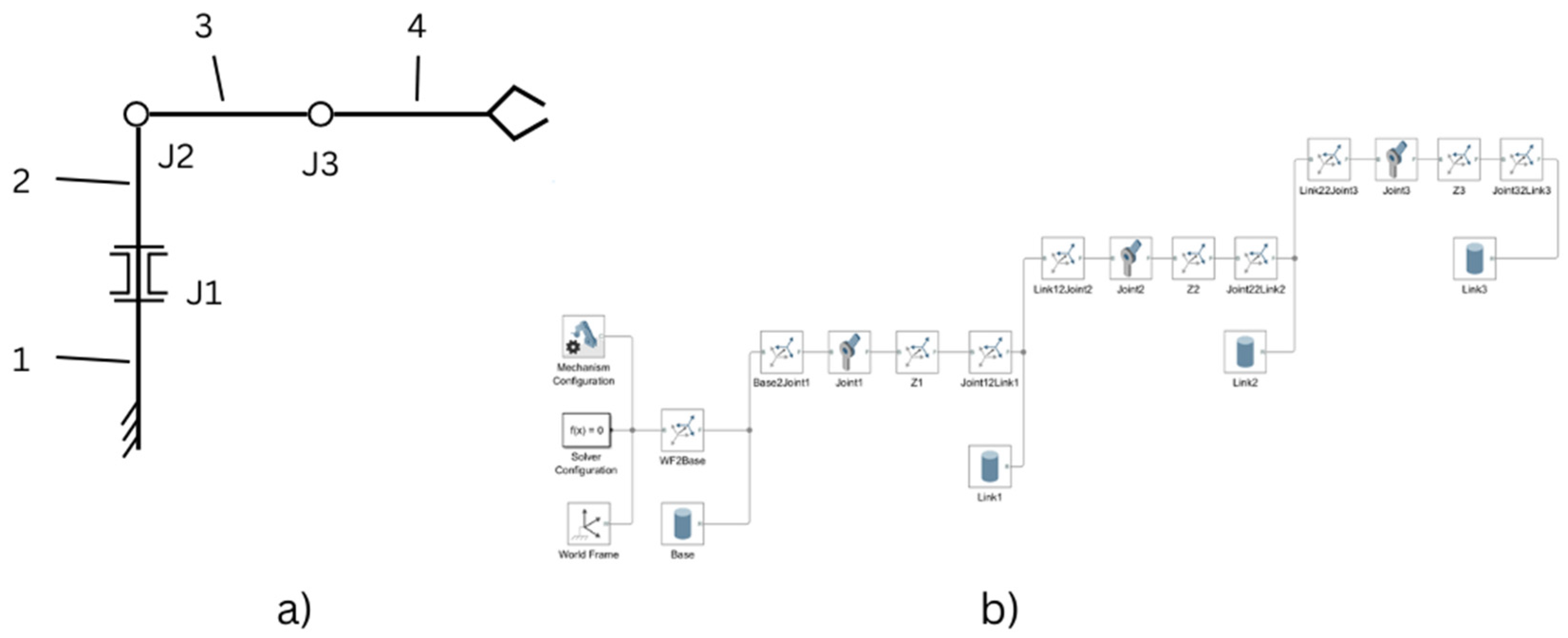
Figure 3.
The components menu in the GUI Editor.
Figure 4.
Push Button (left) and Edit Text (right) parameter lists.
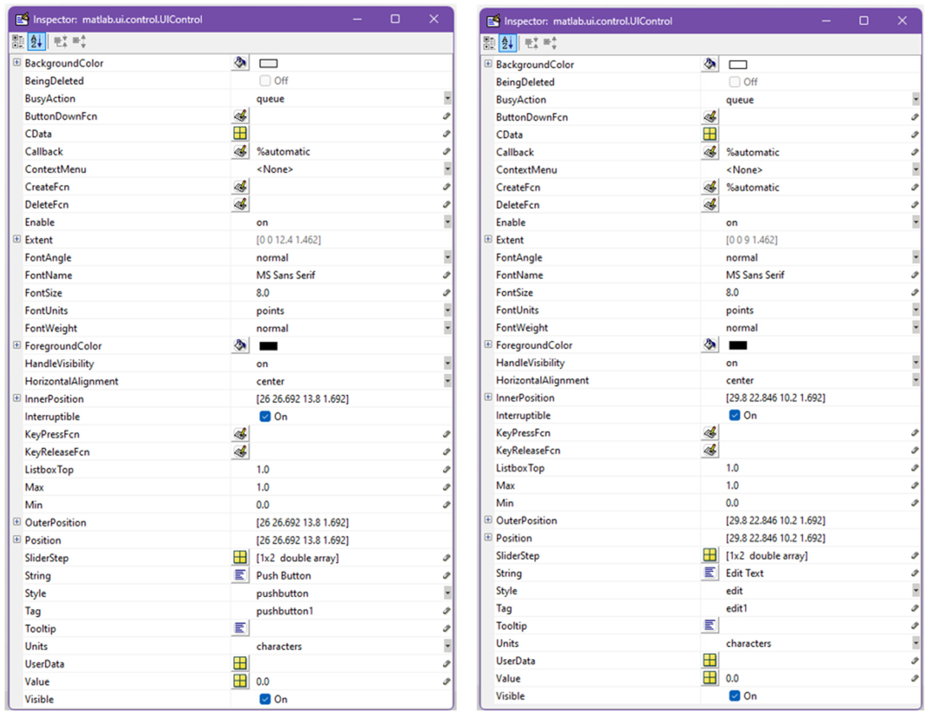
Figure 5.
The user interface.
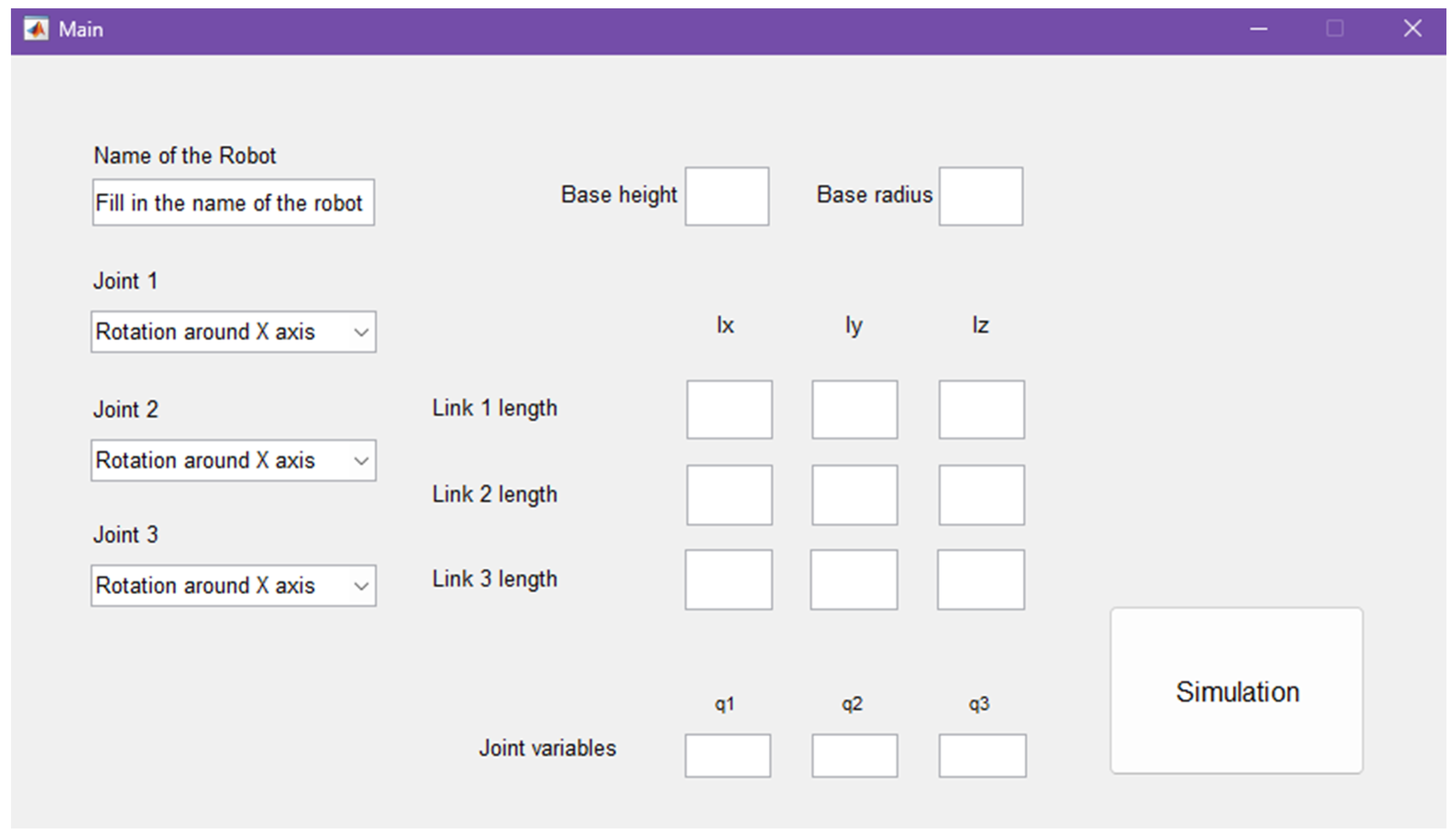
Figure 6.
Function for edit3 - the “Edit Text” box reserved for the name of the robot.
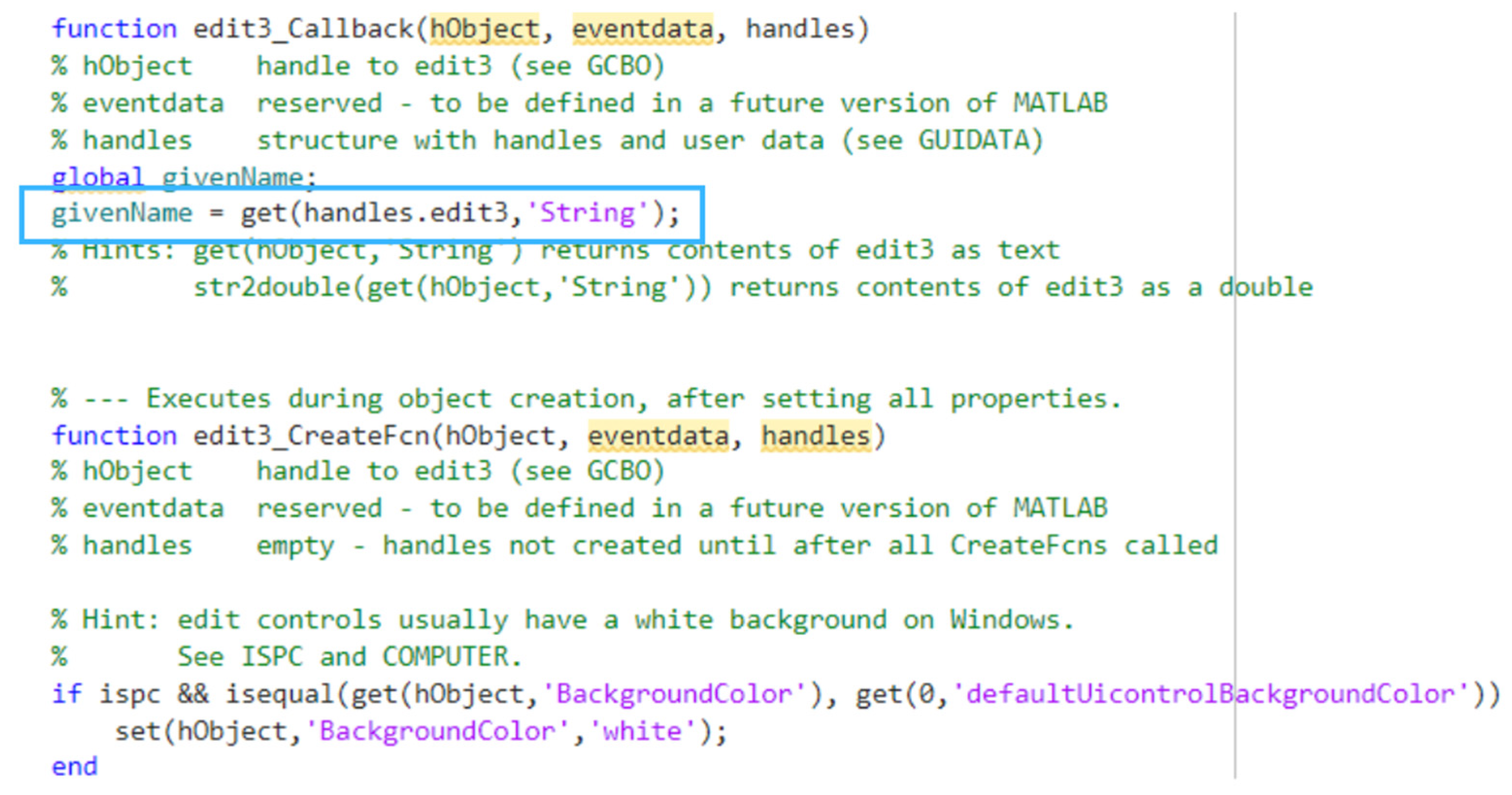
Figure 7.
Function callback for “Push Button”.
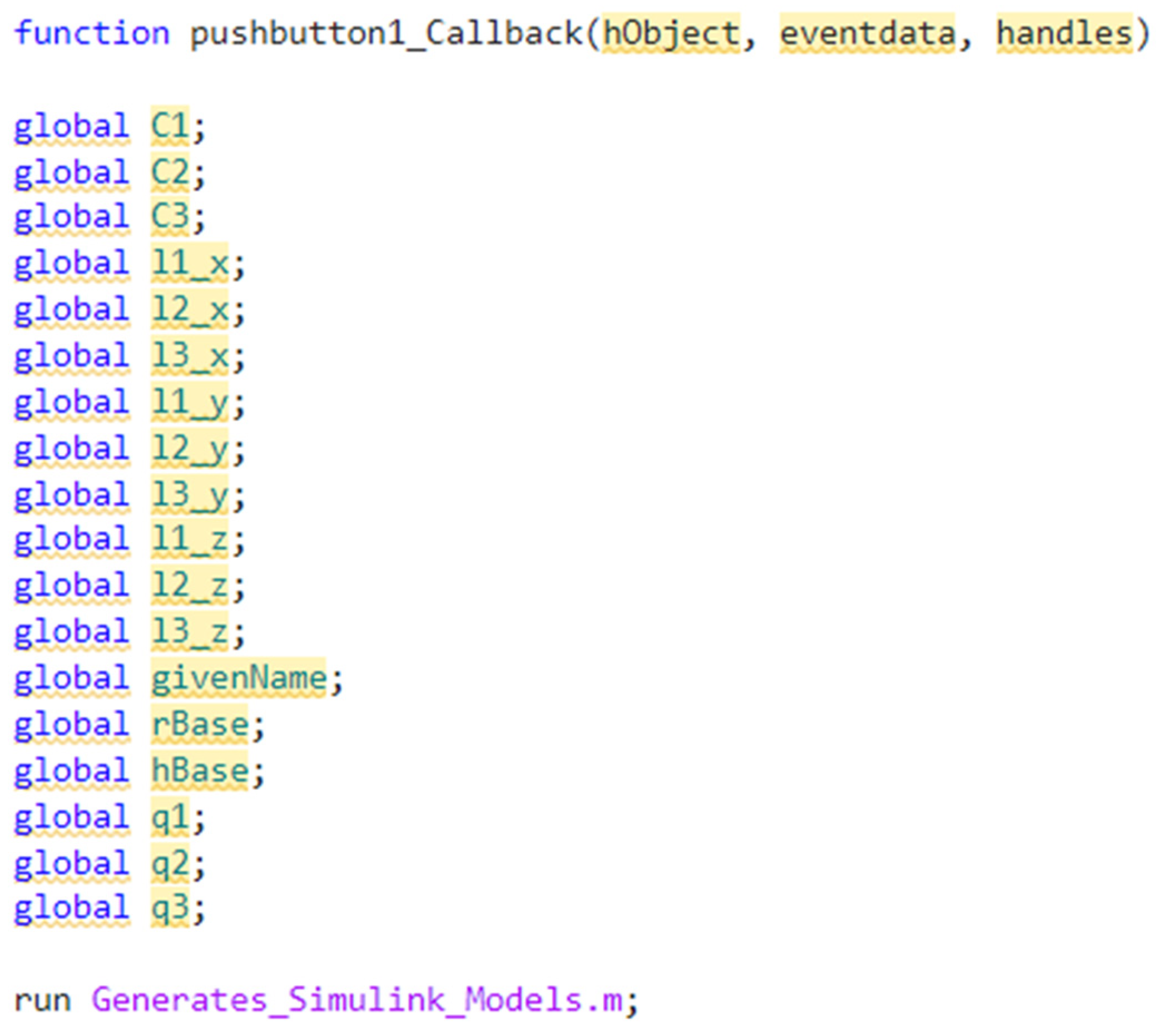
Figure 8.
Structure of Generates_Simulink_Models script.
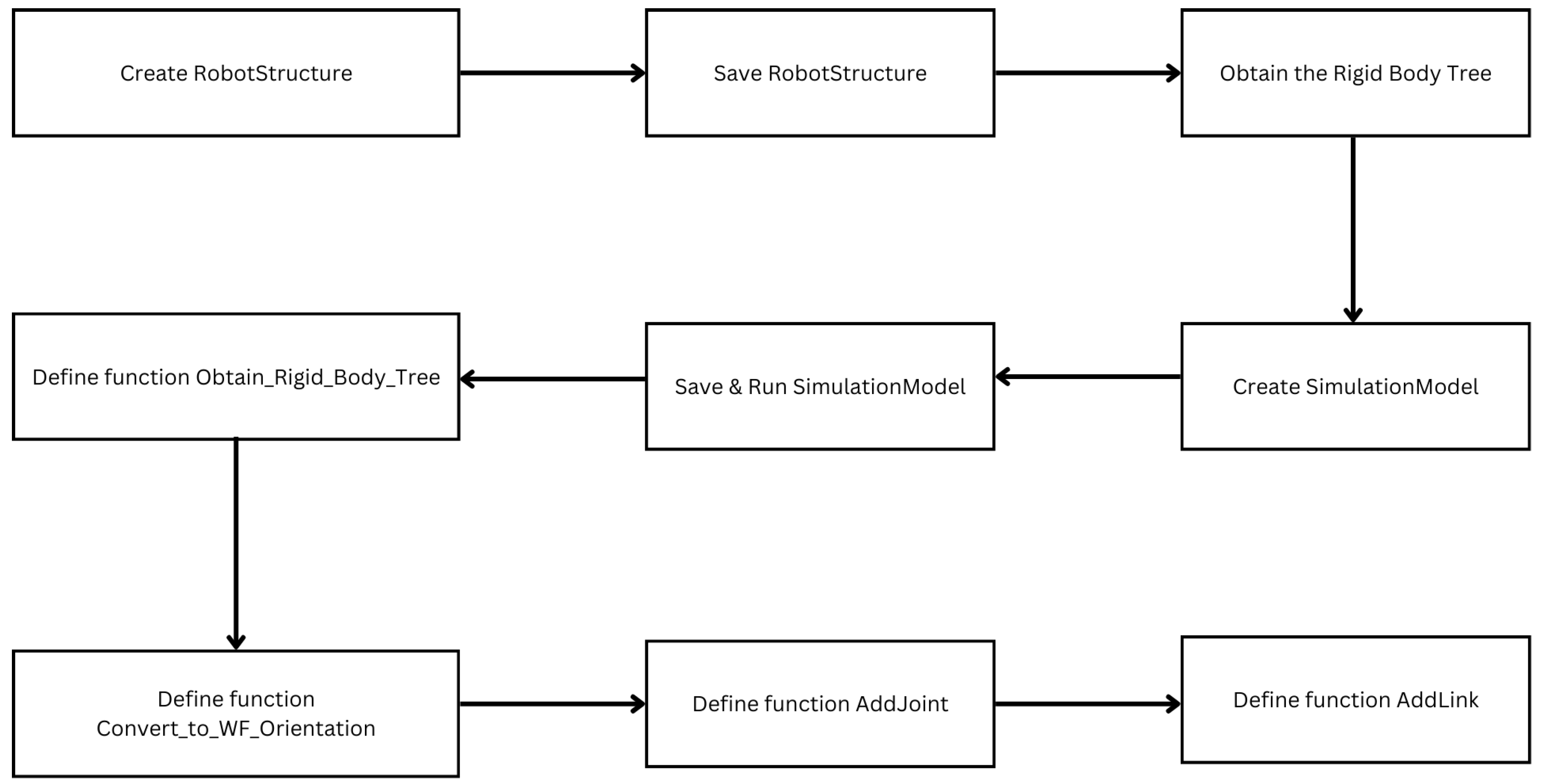
Figure 9.
The three types of Rigid Transform that are proposed. a) Associated with rotation around Z or link length along Z – corresponds to World Frame orientation; b) Associated with rotation around Y or link length along Y; c) Associated with rotation around X or link length along X. All movements are related to WF orientation.
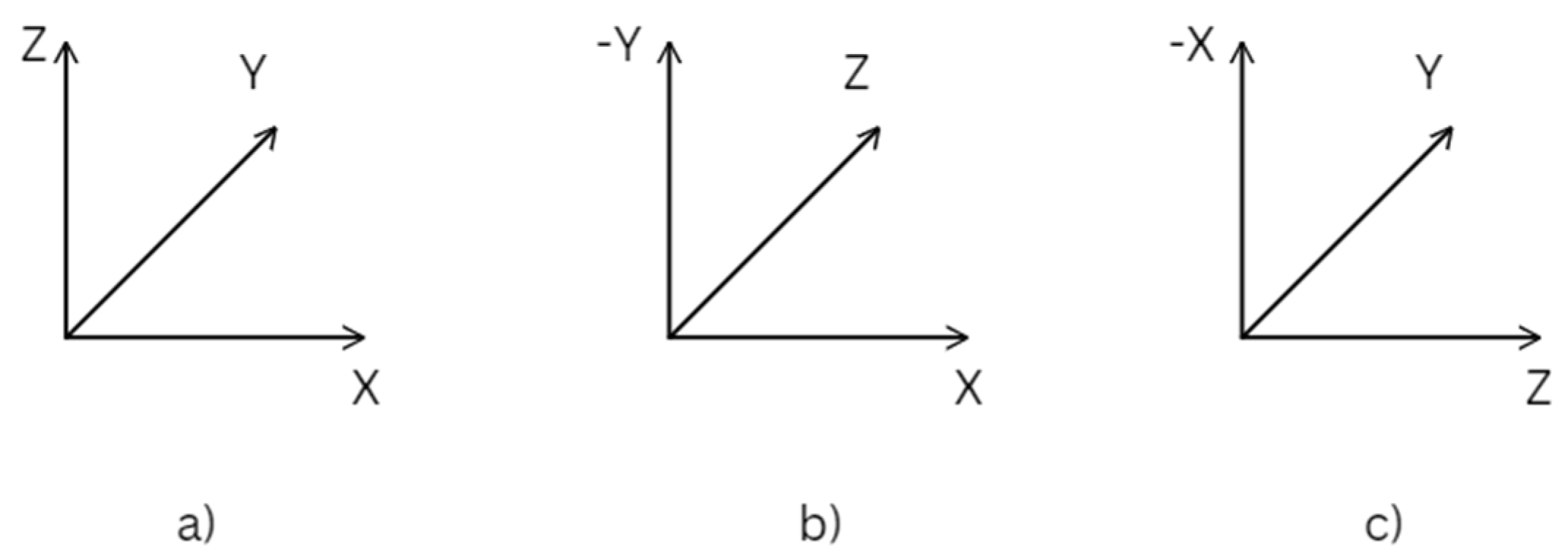
Figure 10.
The necessary transformations to reorient the coordinate system.
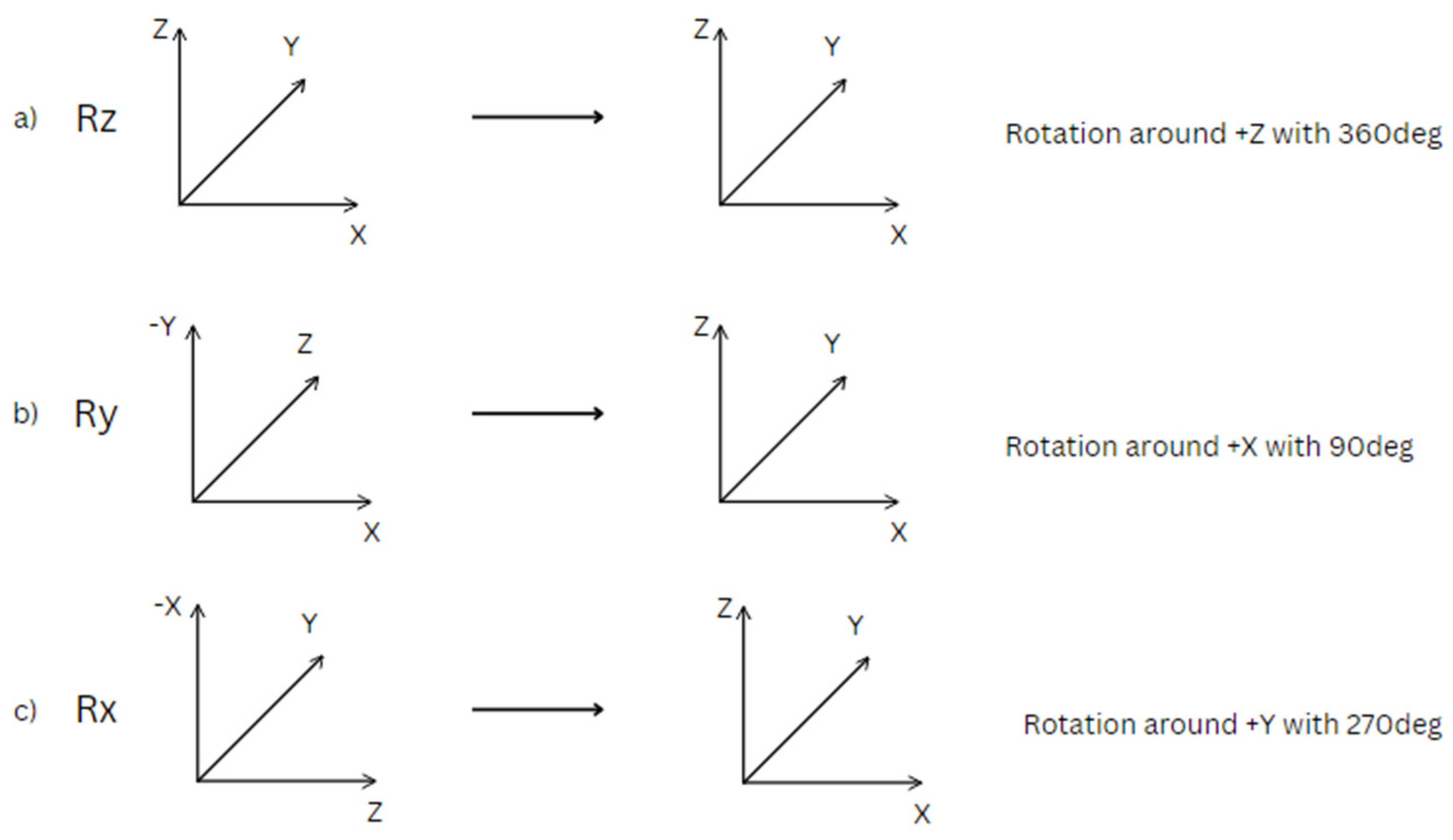
Figure 11.
Structure of a 3DOF using an intermidiate Rigid Transform.
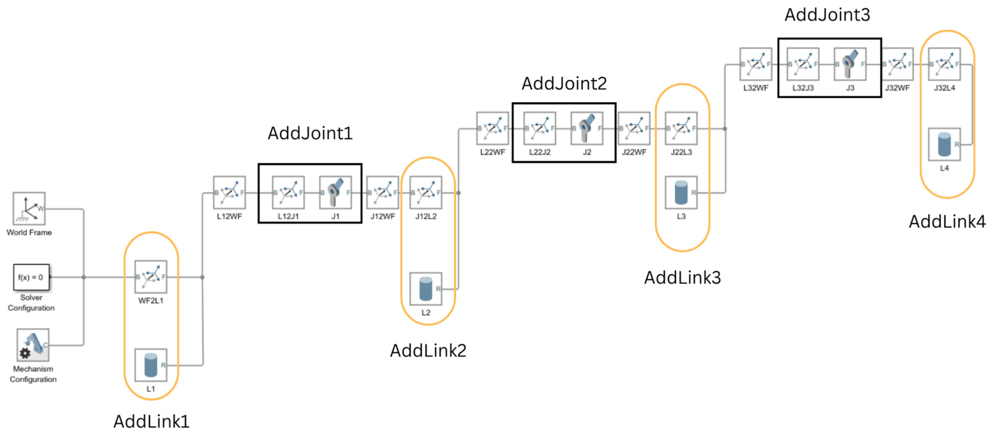
Figure 12.
Convert_to_WF_Orientation function.
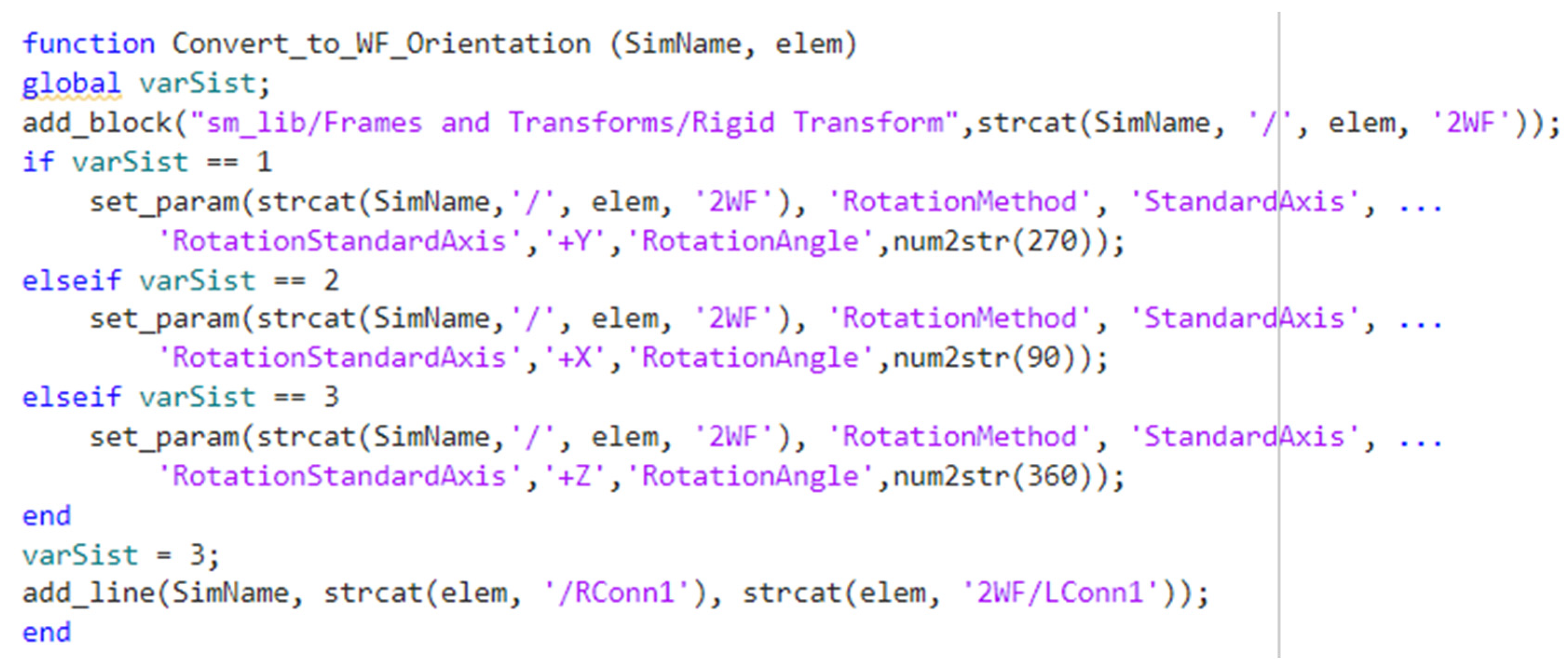
Figure 13.
The scheme of the proposed application that computes forward kinematics.
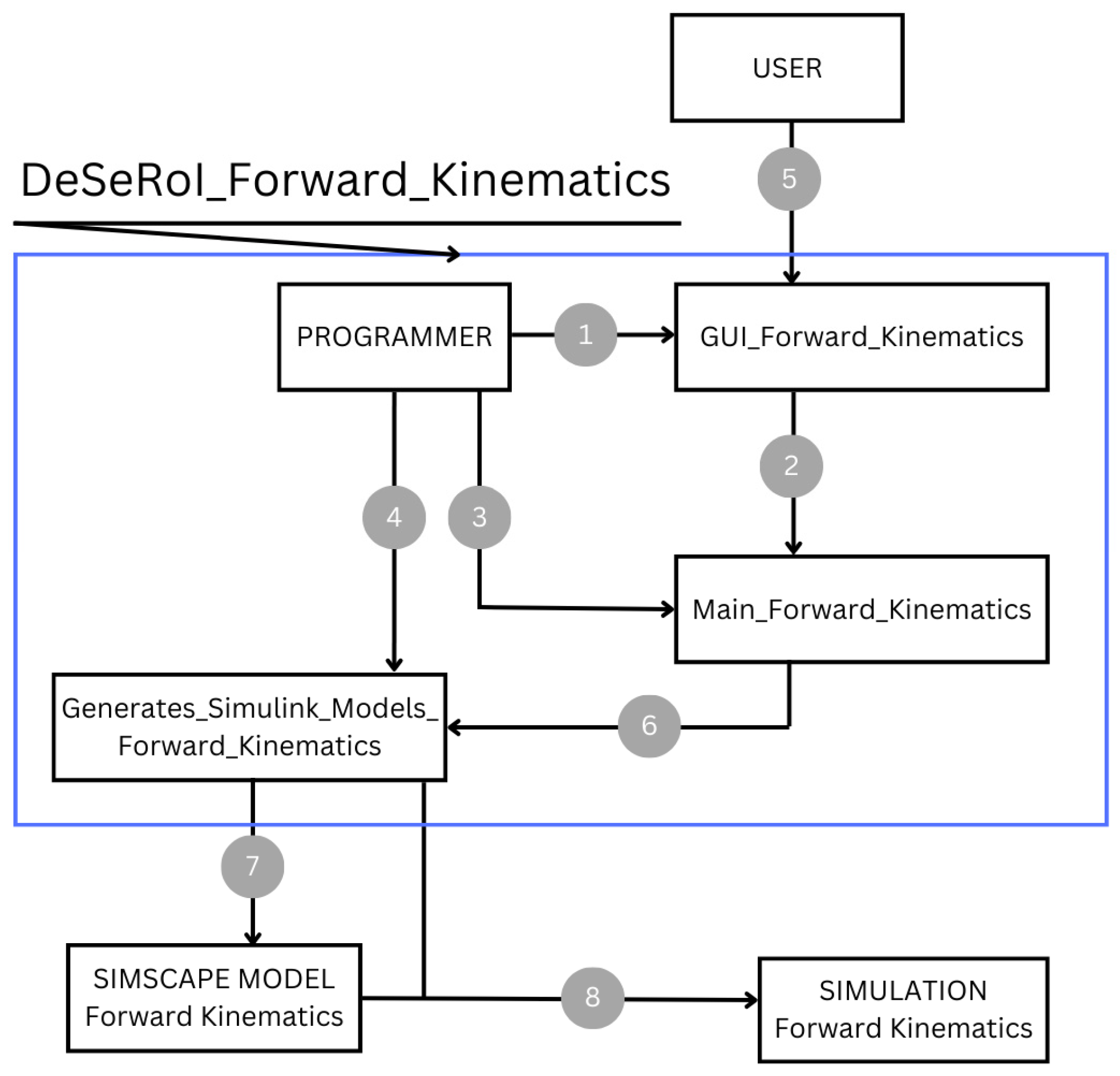
Figure 14.
Configuration of the first serial robot: RzRyRz.
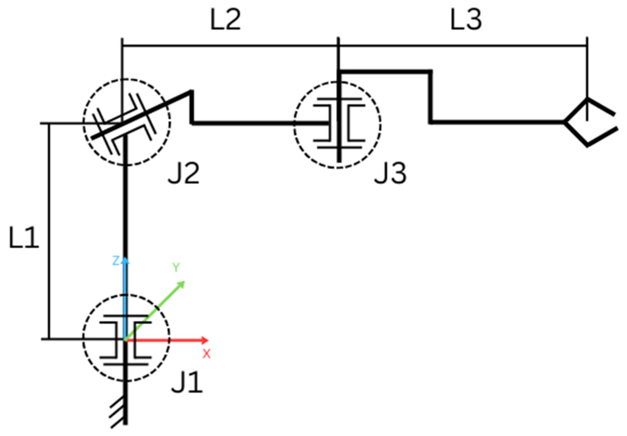
Figure 15.
Input values used for simulating the forward kinematics of the first example.
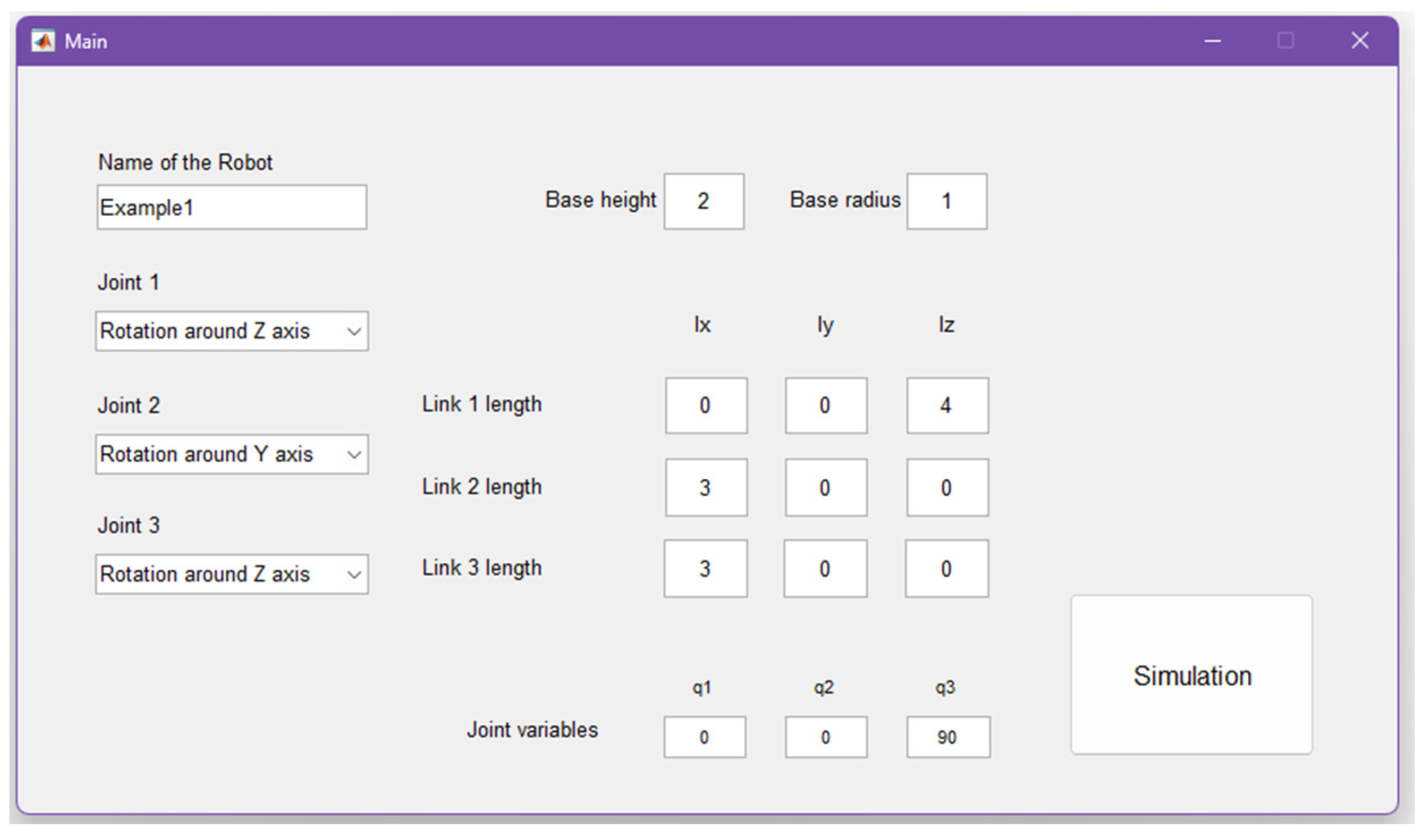
Figure 16.
Simulation results of the RzRyRz serial robot a) Computed position, b) Matrix H1 where the values on column 4 have the following corespondents: 3 – length on X axis (Link2), 0 – length on Y axis, 6 – length on Z axis (Base + Link 1).
Figure 16.
Simulation results of the RzRyRz serial robot a) Computed position, b) Matrix H1 where the values on column 4 have the following corespondents: 3 – length on X axis (Link2), 0 – length on Y axis, 6 – length on Z axis (Base + Link 1).
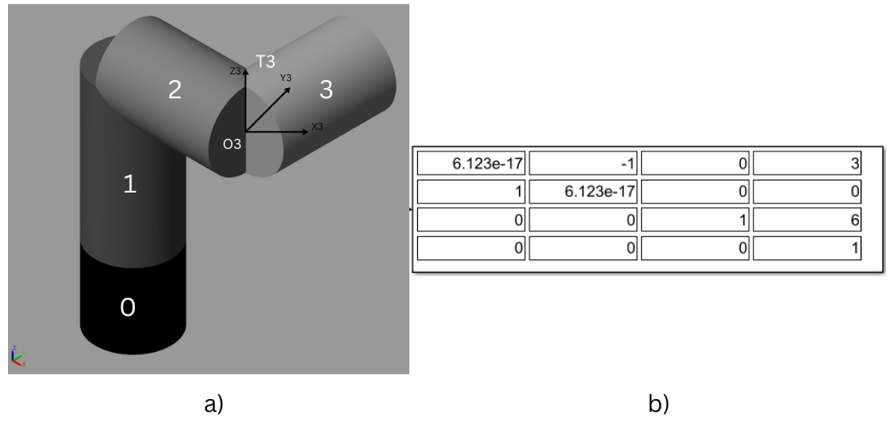
Figure 17.
Configuration of the second serial robot: RzRxRy.
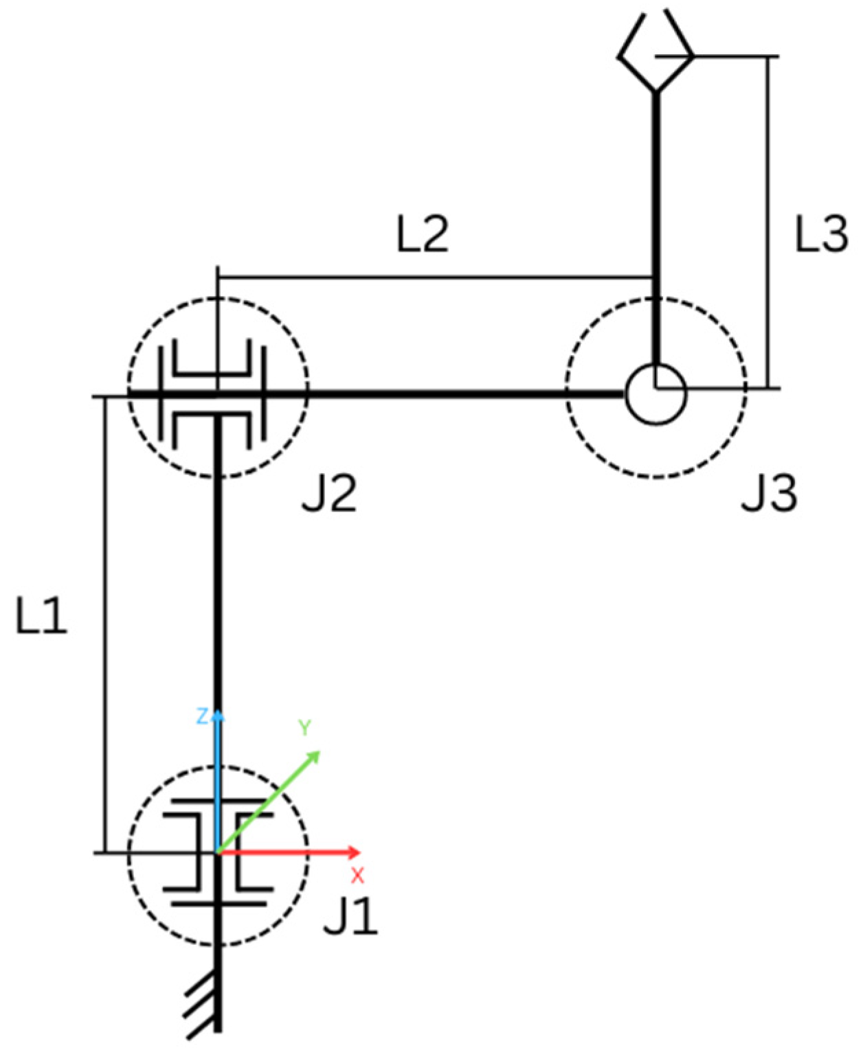
Figure 18.
Input values used for simulating the forward kinematics of the second example.
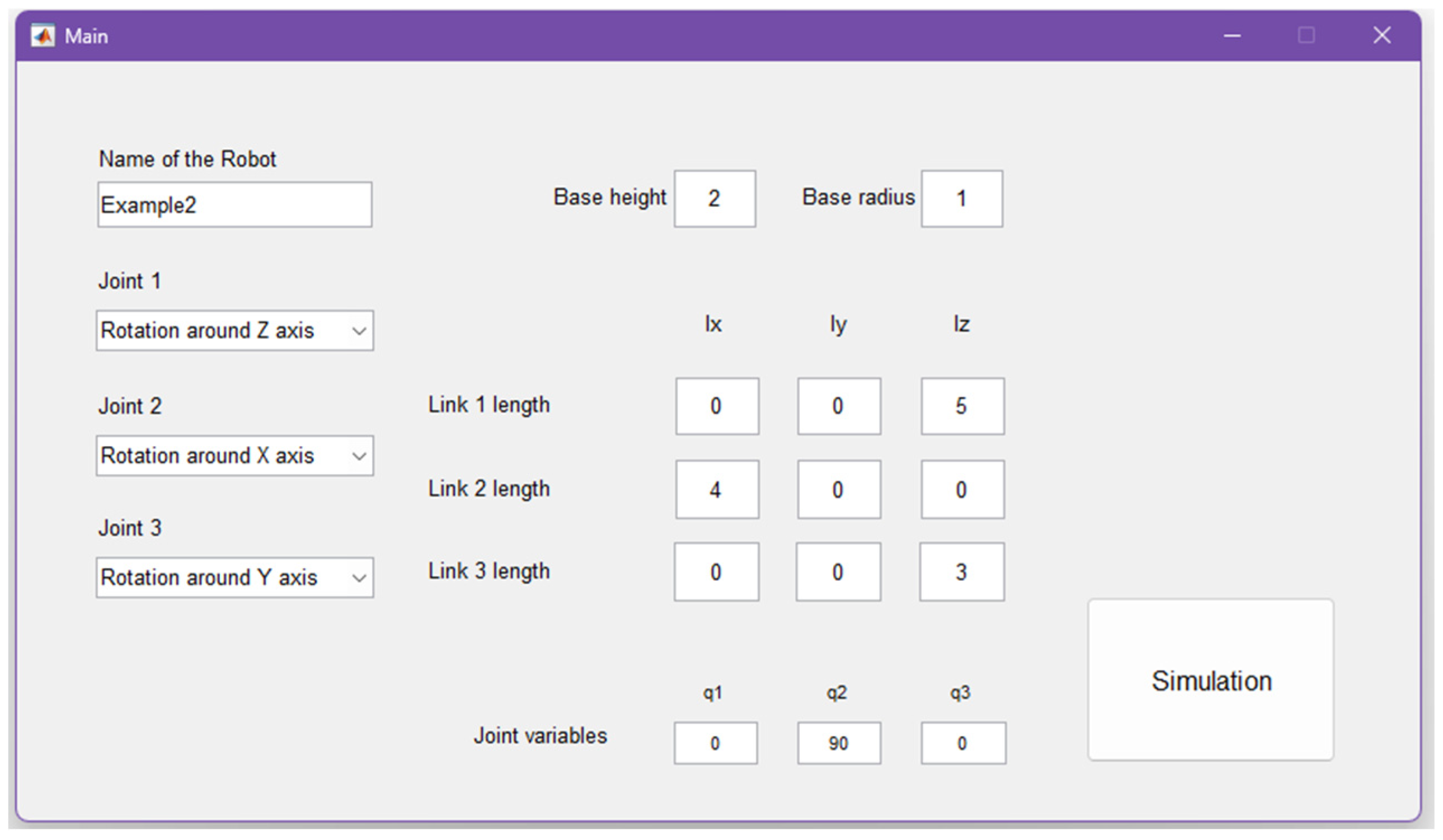
Figure 19.
Simulation results of the RzRxRy serial robot a) Computed position, b) Matrix H2 where the values on column 4 have the following corespondents: 3 – length on X axis (Link2), 0 – length on Y axis, 6 – length on Z axis (Base + Link 1).
Figure 19.
Simulation results of the RzRxRy serial robot a) Computed position, b) Matrix H2 where the values on column 4 have the following corespondents: 3 – length on X axis (Link2), 0 – length on Y axis, 6 – length on Z axis (Base + Link 1).
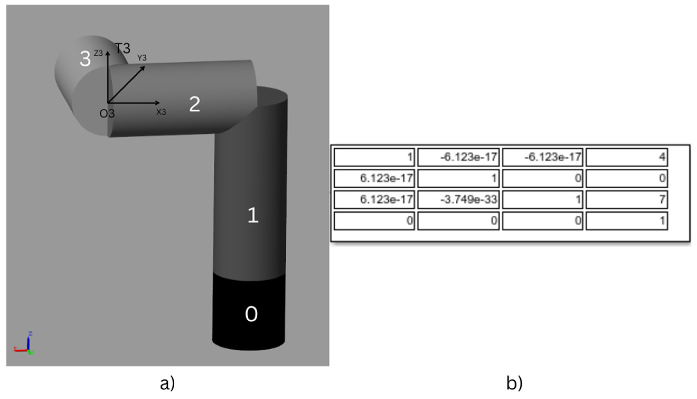

Table 1.
Comparison of the two methods.
| Standard Method | Proposed Method |
| User must build a Simulink Model using the Simscape library that contains the structure of the robot (RobotStructure) | Programmer creates the application that contains a GUI |
| RobotStructure model has to contain blocks representing the links and joints of the robot, connected by coordinate systems, some solver blocks, and the global coordinate system | User runs the main Script (Main) and the graphical interface is open |
| User has to create a MATLAB script where they import the Rigid Body Tree of the robot | User fills in the information about the structure of the robot (name of the robot, type of joints, base parameters, link length, etc.) |
| After the script is run, User has to create a second Simulink model (SimulationModel) | User presses the push button called “Simulation” |
| SimulationModel is going to contain blocks with the values of the joint variables, blocks that convert the measurement unit and are connected to the joints, the structure of the robot, and blocks that solve the kinematics problem | The scripts are going to be run creating two Simulink models: RobotStructure and SimulationModel. SimulationModel going to be run automatically |
| User has to configure the parameters for all of the blocks and make the connections between them | Simulation of the robot can be visualized in MATLAB |
| When finished, SimulationModel must be run | |
| Simulation of the robot can be visualized in MATLAB |
Disclaimer/Publisher’s Note: The statements, opinions and data contained in all publications are solely those of the individual author(s) and contributor(s) and not of MDPI and/or the editor(s). MDPI and/or the editor(s) disclaim responsibility for any injury to people or property resulting from any ideas, methods, instructions or products referred to in the content. |
© 2024 by the authors. Licensee MDPI, Basel, Switzerland. This article is an open access article distributed under the terms and conditions of the Creative Commons Attribution (CC BY) license (https://creativecommons.org/licenses/by/4.0/).
Copyright: This open access article is published under a Creative Commons CC BY 4.0 license, which permit the free download, distribution, and reuse, provided that the author and preprint are cited in any reuse.


