
Submitted:
21 June 2024
Posted:
24 June 2024
You are already at the latest version
Abstract
Mesoscale eddies wield a significant influence on primary productivity in marine ecosystems by regulating nutrient availability, vertical mixing, and phytoplankton growth dynamics. In this study, we tracked and analyzed the effects of mesoscale eddies on net primary productivity (NPP) across the Bay of Bengal (BoB) using remote sensing data. Dividing the Bay into six zones based on mesoscale eddy frequency and distribution, our analysis identified 1880 anticyclonic eddies and 1972 cyclonic eddies during January 2010–March 2020 monitoring period. Cyclonic eddies predominantly occurred in the western part of the bay - along the east coast of the Indian Peninsula; while anticyclonic eddies were also observed, albeit in lesser proportions. Among eddies lasting one-week, anticyclonic eddies comprised approximately 48.81%, while cyclonic eddies constituted approximately 51.19% of the total. Analysis of the NPP distribution across the months revealed intriguing patterns. Mean values of NPP fluctuated throughout the year, with the highest value observed in August (748.51 mg C/m2/day) and the lowest in May (519.26 mg C/m2/day). The findings indicate a complex relationship between eddy distribution and NPP, with Zones 1 and 2 exhibiting a higher occurrence of cyclonic eddies, correlating with greater NPP and its variability. Conversely, Zones 3 and 5 display increased eddy activity despite fewer cyclonic eddies and lower NPP levels. Zone 6 shows reduced eddy activity and NPP, while Zone 4 presents moderate eddy activity alongside lower NPP. In contrast, Zones 3 to 5 exhibit lower NPP levels despite exhibiting heightened eddy activity. This study contributes valuable insights into the dynamics of ocean circulation and the impacts of eddies on NPP, which can inform fisheries management strategies, advances climate resilience measures, expands scientific knowledge, and guides policies related to conservation and sustainable resource utilization.
Keywords:
Mesoscale eddies
; Bay of Bengal
; Primary productivity
; Remote sensing
; Fisheries management
; Ocean dynamics
; Monsoonal wind
; Sustainable resource utilization
1. Introduction
Mesoscale eddies, highly dynamic oceanic features typically spanning tens to hundreds of kilometers in diameter, exhibit distinctive rotational motions and creating circular water flow patterns [1]. These eddies constitute a fundamental dynamic component of the ocean circulation system and play a significant role in the transport of heat, nutrients, and various oceanic properties. They also help in retaining larvae of fish and invertebrates and, in some cases, aggregating pollutants. Their occurrences are widespread across different oceanic regions and often coincide with spatial gradients in temperature, salinity, and biological activity [2]; indicating their pivotal role in shaping local oceanic conditions. Eddy formation is driven by a combination of forces, including wind stress curl, meander separation, baroclinic instability; and that establishes a dynamic equilibrium between pressure gradient force, centrifugal force, and Coriolis force [3]. Eddy formation by means of shedding closed loop meanders from major currents leads to emergence of warm-core and cold-core eddies, representing two primary categories [4]. Warm-core eddies possess elevated temperatures and sea levels at their centers, while cold-core eddies exhibit lower temperatures and reduced sea levels in their cores [5,6]. These distinct characteristics not only influence the thermal and dynamic properties of surrounding oceanic environment, but also impact the distribution and behavior of marine life, making them essential for understanding oceanic ecosystems and climate dynamics [7] on an ocean-wide scale.
In the context of the Bay of Bengal (BoB), mesoscale eddies are vital components of its circulation and mixing dynamics. The BoB undergoes a semiannual reversal of monsoon wind system, in sync with the climate pattern of southern and southeastern Asia. From June to September, southwesterly winds (referred to as the summer/southwest monsoon) prevail, while from November to February, northeasterly winds prevail (known as the winter/northeast monsoon). These wind patterns also result in a seasonal reversal of ocean circulation pattern in the BoB. The Bay also experiences high precipitation; > 2000 mm/year[8]. Additionally, runoff from peninsular rivers contributes approximately 1.625×10¹² cubic meters per year. The associated suspended sediment discharge from river runoff into the Bay is estimated to reach approximately 1.382×10⁹ metric tons per year [9]. Cheng et al. [10] studied the formation and propagation of mesoscale eddies in the BoB that would originate near the eastern boundary and spread southwestward with a lifespan of 30 to 120 days. Eddies also arise in the western portion of the BoB due to baroclinic instability of the East Indian Coastal Current (EICC); whereas eddies in the central BoB are remotely pushed by equatorial Kelvin waves, coastline geometry, and nonlinear Rossby wave propagation [9,11]. Kumar et al. [11,12] reported nine cold-core eddies that resulted from the instability of EICC in the central and western BoB, based on hydrographic and satellite data. Cheng et al. [9] also found that eddies in the BoB are predominantly driven by equatorial zonal winds, with the majority of eddies having lifespans in the range of 30-120 days and originating near the eastern border and aligning with the thermocline’s vertical motion. Several studies have employed satellite altimetry data to identify and track mesoscale eddies in the BoB, particularly during the inter-monsoon period [13,14,15]. In the summer season, anticyclonic gyres are present in the western BoB due to the occurrence of higher temperature and salinity lingering from the spring season, along with decreasing salinity during autumn [11,13,14,15]. Notably, the western boundary is more conducive to eddy formation, which can be attributed to enduring baroclinic instability of the EICC; whereas the southern Bay experiences fewer eddies, potentially due to a weaker Coriolis force at approximately 6°N [16,17,18]. Moreover, some studies have revealed that variations in eddy genesis and propagation correlate with monsoonal changes in the western BoB, which features shallow bathymetry and significant freshwater influx from the Godavari and Krishna Rivers into the western BOB during the post monsoon period [13,19].Advection of freshwater plumes farther south by the EICC from the northern BoB forms a barrier layer, further influencing eddy dynamics along eastern BoB [16,20,21].
Baroclinic instability induced by Rossby waves also supports eddy formation in the western BoB. Roman-Stork [22] and Kumar [23] both highlighted the role of baroclinic instability in the formation of eddies in the western BoB. Roman-Stork [22]) specifically links this instability to the influence of coastal Kelvin waves and westward propagating Rossby waves, while Kumar [23] emphasizes the impact of opposing currents and wind stress curl. They affect ocean instabilities, enhancing them in winter and diffusing them in summer and modulating coastal circulations, weakening the EICC in winter and strengthening it in summer. Mukherjee et al. [24] demonstrated and examined how the Andaman and Nicobar Islands influence mesoscale eddy formation in the western BoB. Their findings indicate a significant reduction in the number of westward propagating eddies due to the presence of the Archipelago.
In a recent study by Gulakaram et al. [25], during the period of 1993-2016, a total of 571 anticyclonic tracks and 560 cyclonic tracks were identified in the BoB, encompassing 3,936 individual anticyclonic eddies and 3,840 individual cyclonic eddies. Research has demonstrated that cold-core eddies can displace the nutricline upward along isopycnal surfaces, infusing nutrients into the surface layer. This vertical transport process has the potential to enhance productivity and promote the downward export of organic carbon [26,27,28]. Kumar et al. [11] suggested eddy pumping as a potential method of vertical nutrient transport from the halocline to the euphotic zone during the summer monsoon, when the upper ocean is strongly stratified. Sarma et al. [29] reported high nutrient concentrations associated with cyclonic eddies in the BoB and vice versa for anticyclonic eddies.
Considering these complex circulation dynamics, the primary objective of this study is to comprehensively characterize and analyze mesoscale eddies across the entirety of the BoB using multiple time series datasets. Despite significant prior research contributing to our understanding of mesoscale eddies and their behavior within the BoB, knowledge gaps remain regarding their influence on various regions, including the eastern coastal waters of India, the coastal waters of Bangladesh affected by freshwater input from three major rivers, the Andaman Sea, and deeper waters, as well as their impact on the vertical distribution of biogeochemical properties, particularly in the northern and southern reaches of the BoB. This study further explored the underlying mechanisms governing eddy formation and its spatiotemporal variability to gain a deeper understanding of their implications for marine ecology. Within the context of the BoB, this research holds particular significance because it illuminates the dynamics of a critical marine ecosystem, informs fisheries management strategies, advances climate resilience measures, contributes to the expansion of scientific knowledge, and informs policies related to conservation and sustainable resource utilization.
2. Materials and Methods
2.1. Study Area
The study area covers the BoB and most of the Andaman Sea (see Figure 1). The BoB is the northern extension of the Indian Ocean and is surrounded by land except in the southern region, where it is open to the influence of the Indian Ocean. The geographic location of the study domain is between 0°N and 23°N and between 80°E and 100°E, and the area covers approximately 4.087×10⁶ km2, with a maximum depth of approximately 4500 m [30]. It is surrounded by India and Sri Lanka in the west, Bangladesh in the north, Myanmar, and the northern Malay Peninsula in the east. The regional climate is heavily influenced by monsoons, with the southwest monsoon prevailing from June to September and the northeast monsoon prevailing from November to April. Additionally, the BoB is known for its tropical cyclones, with approximately 5 to 6 cyclones originating annually, some of which can be severe and cause landfall in India, Bangladesh, and Myanmar. Several major rivers drain into the BoB, viz., Ganges, Brahmaputra, Mahanadi, Godavari, Krishna, Irrawaddy, Meghna, Karnaphuli, etc.
2.2. Data Sources
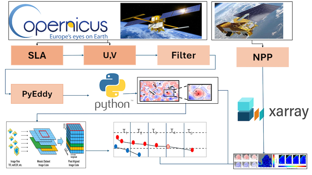
Mesoscale eddies in the BoB were identified from the analysis of postprocessed and gridded daily sea surface height anomaly data from January 2010 to March 2020. This dataset was obtained from the Copernicus Marine Environment Monitoring Service (CMEMS) and is available at https://cds.climate.copernicus.eu/cdsapp#!/dataset/satellite-sea-level-global?tab=overview), with a spatial resolution of 0.25° x 0.25°. To visualize seasonal surface currents, the method involved iterating through three distinct seasons: premonsoon (March- May), southwest monsoon (June to September), and winter (October to December). For each season, the u and v components of velocity were extracted from the dataset, and the velocity magnitude was computed. A longitude-latitude grid was created, and streamlines representing flow direction were plotted using the streamplot function. Additionally, the velocity magnitude was depicted as a color mesh using the pcolormesh function of Matplotlib [31].
2.3. Eddy Identification
Eddy tracking, identification, and associated property identification were conducted using the Python package (https://github.com/AntSimi/py-eddy-tracker). This package uses daily 0.25° × 0.25° resolution gridded sea level anomaly (SLA) data [32] as input. Recent advancements in oceanographic research have led to the widespread utilization of three primary algorithms for mesoscale eddy tracking. These methodologies encompass the geometric approach [33,34,35], which relies on the characterization of closed contours in SLA data based on their shape and size; the Okubo-Weiss (OW) method [36], which leverages vorticity and strain derived from the flow field as computed from SLA; and the wavelet method [37], which is rooted in spectral analysis through wavelet transformation of SLA data. For our research, the emphasis was placed on the OW and geometric methods, with the procedures following the framework established by [34,36,38]. This method has already been reported in several studies focusing on the detection of mesoscale eddies in the Tasman Sea [39], Mediterranean Sea [40], and global ocean [36]. Therefore, an automated eddy detection algorithm based on the OW parameter that has been tested for diverse oceanic and regional seas was implemented in this study. The OW parameter is defined as
where and, ω are the normal strain, shear strain (normal component and shear component of the strain tensor), and vorticity (vertical component of the relative vorticity), respectively.
where u and v are the zonal and meridional geostrophic velocity components, which are calculated from the sea surface height anomaly (SSHA) as follows:
where g is the gravitational force, f is the Coriolis factor and x and y are horizontal coordinates. Generally, a threshold of W=0 is set such that OW < 0 represents vorticity and eddy-dominated regions. The negative values of OW are in good agreement with the eddy cores detected. The choice of the threshold for the OW parameter defines the precision and ability to identify an eddy. Therefore, we utilized OW < -0.2 σw as a threshold value to determine the region of eddy core where σw is the standard deviation of the OW [41].
3. Results and Discussion
Our extensive analysis spanning from January 2010 to March 2020 revealed interesting patterns in the frequency and spatial distribution of mesoscale eddies in the BoB. Remarkably, both cyclonic and anticyclonic eddies were found to be prominent features, each comprising approximately half of the observed eddy count (Figure 2). Specifically, our study identified approximately 1880 anticyclonic eddies and 1972 cyclonic eddies within the BoB during the analysis period (Figure 3). This finding surpasses previous research [42], as we have accounted for the lifespan of eddies lasting up to a week. Further analysis revealed distinct spatial distributions of cyclonic and anticyclonic eddies within the BoB. Cyclonic eddies were primarily prevalent in the western part of the bay (Figure 2 and Figure 3) along the east Indian coast, whereas anticyclonic eddies were observed but in lesser proportions. The eddy frequencies visible to the east of Sri Lanka, along the western boundary of the BoB in Figure 2, are clearly identifiable. Due to its strategic positioning and potential to redirect the pathway of the EICC, the consistent presence of this eddy is a significant finding of this research. This distribution pattern suggests potential differences in the underlying ocean dynamics and atmospheric interactions that drive the formation and propagation of these mesoscale eddies. These findings are also consistent with those of Cui et al.[43] and Trott and Subrahmanyam [44]. The prevalence and distribution of eddies within the BoB are influenced by various factors, including oceanic local currents, atmospheric circulation patterns, seasonally varying air-sea interaction dynamics and local bathymetry [13]. Cyclonic eddies often result from the convergence of oceanic currents or interactions with topographic features. These eddies can also modulate the intensity of tropical cyclones, with their presence resulting in significant sea surface temperature cooling and changes in latent heat flux supply [45]. The formation of subsurface cyclonic eddies in the BoB, such as the one observed in the northwestern region in 1984, can be attributed to baroclinic instability at the interface of opposing boundary currents [46]. Anticyclonic eddies, on the other hand, may arise from the divergence of currents or the influence of atmospheric systems, such as cyclonic storms or monsoon winds [21,47]. These warm-core eddies significantly impact the ocean heat content in the BoB. Studies have shown that these eddies can alter the vertical distribution of heat, thereby influencing the overall thermal structure of the ocean [48]. This process is crucial for understanding the thermal dynamics and energy budget of the BoB. The westward propagation pattern observed in our study suggests potential interactions between eddies and adjacent oceanic features, such as coastal upwelling zones or boundary currents. These interactions can significantly impact nutrient transport, heat flux, and planktonic community structure within the BoB, ultimately influencing marine ecosystem and fisheries productivity [49].
3.1.1. Mesoscale Eddy Life Span, Frequency, and Track Analysis
Analysis of eddy lifespans revealed notable trends in the distribution of anticyclonic and cyclonic eddies across different time scales. For eddies lasting 1 week, percentage of anticyclonic eddies is approximately 48.81%, while cyclonic eddies constitute approximately 51.19% of the total. Similarly, for eddies with a lifespan of 4 weeks, the proportions of anticyclonic and cyclonic eddies remain close, with percentages of approximately 49.00% and 51.00%, respectively. This suggests that cyclonic eddies tend to have extended lifetimes and greater energy levels [50]. However, as the lifespan of eddies increases, their distribution shifts. For instance, for 12-week-long eddies, the percentage of anticyclonic eddies decreases to approximately 41.51%, while that of cyclonic eddies increases to approximately 58.49%. This trend continues with 16-week-long eddies, where anticyclonic eddies constitute approximately 44.23%, and cyclonic eddies increase to approximately 55.77%. Interestingly, for 24-week-long eddies, the ratio shifts significantly, with that of anticyclonic eddies comprising 56.25% and that of cyclonic eddies decreasing to 43.75%. The most pronounced shift is observed for 30-week-long eddies, where the percentage of anticyclonic eddies decreases to 16.67%, while that of cyclonic eddies increases dramatically to 83.33% of the total. This finding underscores the dynamic and transient nature of mesoscale eddy formations within the study area. Furthermore, our investigation revealed distinct patterns in the spatial distribution and propagation direction of these eddies. Specifically, we observed that the majority (91%) of all eddies propagated west/southwestward (Figure 3) along the western slope of the Andaman Archipelago, potentially influenced by the interaction between prevailing ocean currents and coastal topography, with concentrations primarily observed in the Andaman Sea and the western and central zones of the BoB (86-93E, 13-16 N). This spatial distribution highlights the importance of regional circulation dynamics and atmospheric forcing in the evolution and transport of eddies in the BoB (Figure 3). This finding aligns with the results reported by Chen et al. [17].
The frequencies of mesoscale anticyclonic and cyclonic eddies in the BoB exhibit clear spatial patterns. Newly formed cyclonic eddies tend to have a scattered distribution across the BoB, while anticyclonic eddies are more commonly found along the shelf and are concentrated in the western boundary and the south-eastern region (around the Andaman Sea) (Figure 4).In the western BoB, baroclinic instability of the EICC and turbulent energy within meanders contribute significantly to eddy formation; accounting for 30-50% of sea level variability [51]. The eastern bay experiences the highest number of eddies, with coastal Kelvin and Rossby waves being key mechanisms for generating small-scale eddies [10]. Cheng [48] further supports this, identifying high eddy activity in the western BoB and attributing it to barotropic/baroclinic instability. Gonaduwage [52] adds to this by identifying baroclinic instability as a key factor in the increased eddy kinetic energy and transport in the western BoB. This highlights the dynamic and complex nature of eddy formation in the BoB, driven by different physical processes in the western and eastern regions [17,48]. The studies by Chen et al. [17], Chang et al. and Jinglong et al. [48,53] highlighted the significance of baroclinic instability and wind stress in affecting the variability of eddies in the BOB.
Analysis of histogram on the lifespan of mesoscale eddies revealed a relative dominance of short-lived eddies (both cyclonic eddies, represented by blue bars, and anticyclonic eddies, represented by red bars, as shown in Figure 5) across all years of observation (top left plot). This dominance is evident from the decreasing frequency of eddies with increasing lifespan. Despite both types exhibiting an increasing trend in cumulative occurrence (top right plot), the blue line in the bottom left plot, representing the ratio of cyclonic to anticyclonic eddies within each lifetime bin, consistently surpassed the green line, indicating equal distribution. This preference for short-lived cyclonic eddies further manifested in the bottom right plot, where the blue line depicting the cumulative ratio steadily increasing over time, suggesting a potential shift in BoB eddy dynamics favoring shorter-lived cyclonic events [22].
3.1.2. Mesoscale Eddy Propagation Analysis
Eddy propagation distances vary directly with their lifespan, with longer-duration eddies exhibiting greater spatial coverage. For eddies lasting 1 week, the mean propagation distance is approximately 72.26 km, with a maximum of 337.03 km and a minimum of 6.75 km. As the duration of the eddy increases to 4 weeks, the mean propagation distance increases to approximately 242.31 km, with a maximum of 741.72 km and a minimum of 45.29 km. Similarly, for 8-week-long eddies, the mean propagation distance further increases to approximately 392.66 km, with a maximum of 1164.53 km and a minimum of 107.82 km. In contrast, for 12-week-long eddies, although the mean propagation distance remains relatively high at approximately 536.33 km, there is a notable increase in variability, with a maximum of 936.44 km and a minimum of 262.54 km. Interestingly, for 16-week-long eddies, the mean propagation distance remains consistent at 661.83 km, indicating a stable pattern of propagation over this duration. However, for longer durations, such as 20 weeks and 24 weeks, there was a substantial increase in the mean propagation distance to approximately 884.87 km and 1187.43 km, respectively (Figure 6).
In the case of cyclonic eddies, the mean speed radius is 76.14 km, with a maximum of 308.6 km and a minimum of 20.4 km. Similarly, the mean of the speed average is 0.25 cm/s, with a maximum value of 1.07 cm/s and a minimum of 0.04 cm/s (Figure 7). In the context of anticyclonic activity, the statistical analysis revealed that the mean speed radius was 80.62 km, with a maximum value of 351.3 km and a minimum value of 22.15 km. Similarly, the mean speed average is determined to be 0.24 cm/s, ranging from 0.04 to 1.11 cm/s.
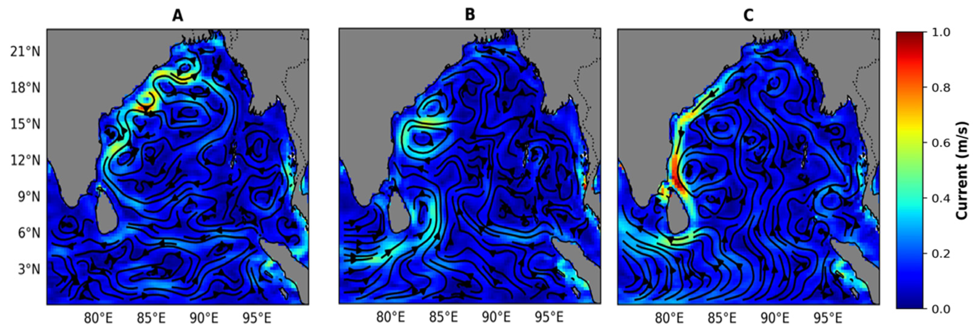
Ocean-scale circulation (Figure 8) in the BoB is unique and more complex than other regional bays and seas in the world because it is dominated by the seasonally reversing monsoon wind system; southwesterly winds during summer months (June–September) and northeasterly winds during fall (October–December). The EICC flows northward during the Inter-monsoon season, beginning in February, and becomes extremely strong in March and April because of anticyclonic eddies forming and spreading westward (see Figure 8A). As the southwest monsoon arrives, the EICC continues to flow north along the southern portion of the Indian Peninsula, but the current becomes erratic as it approaches the head Bay region (Figure 8B). This can be explained by the anticyclonic and cyclonic eddies developing in succession throughout the summer monsoon season. Fall arrives (October to December), and EICC begins to flow southward with current speed reaching 1 m s−1 in the upper 70-80m. Low-salinity water from the head bay area is transported south by the EICC, and high-salinity water is brought into the bay by the subsurface northward flow during this season. In contrast, eastern coast experiences moderate currents, typically ranging between 0.2 and 0.6 m/s. BoB’s flow dynamics is also controlled by the equatorial wind and current system, which is modulated by the Indian Ocean Dipole (IOD) and is linked to El Niño–Southern Oscillation (ENSO), which originates in the equatorial–Tropical Pacific [25,54]. During the spring and summer, the BoB receives a large influx of water and sediments from seven main rivers that originate in the Himalayas and Indian Subcontinent. Several studies have documented the formation, distribution, propagation, and lifecycle of mesoscale eddies in the BoB to comprehend their circulation pattern and impacts. While cyclonic eddies predominate during the northeast monsoon, several significant anticyclonic eddies regulate the circulation of the bay throughout the spring (March–April) inter-monsoon period [12,17,19,49]. The EICC, which shows a northward flow along the southern portion of the east coast of India and a southbound flow along the northern part, primarily influences the surface circulation in the BoB. The formation of the EICC has been largely attributed to seasonal coastal Kelvin waves, as demonstrated by a study by Cheng et al. [8]. Furthermore, the EICC plays a crucial role in regional hydrodynamics. East of Sri Lanka, the EICC bifurcates, with one part continuing along the Sri Lankan coast and the major part flowing eastward into the BoB (Figure 8). This bifurcation results in the offshore transport of chlorophyll-rich, low-salinity water from the Sri Lankan coast This bifurcation of the EICC occurs annually, driven by an anticyclonic eddy impinging on the Sri Lankan coast. However, it is notably absent during IOD years [55]. The main sources of eddies include interannual wind patterns and nonlinear interactions with the morphological features and bathymetry of the continental shelf. Particularly near the western boundary (Figures 2 and 8), these eddies propagate southwestward for durations ranging from 30 to 120 days [50,51]. Strong seasonal variability characterizes the upper layer circulation in the BoB, with anticyclonic flow predominating during the early southwest monsoon in April and May and cyclonic flow dominating during the early northeast monsoon in November. This variability is closely tied to the Indian monsoon, which is fueled by dry northeasterly winds cooling during the winter and southwesterly winds, warmth, precipitation, and enhanced freshwater discharge from rivers during the summer and is intimately linked to this fluctuation [27].
4. Conclusions
Mesoscale eddies in the BoB were studied in terms of their lifespan and frequency using satellite altimetry data spanning from 2010 to 2020. Employing a hybrid algorithm that incorporates both physical and geometrical properties, we have detected and tracked eddies in the study area. Our study thoroughly examines the statistical characteristics, variability, and properties of both anticyclonic eddies and cyclonic eddies over a 10-year period. The results revealed a distinct relationship between the level of eddy activity and a myriad of regional forcings that caused them, including the role of Rossby waves and Kelvin waves propagating across BOB. Cyclonic eddies, prevalent in western and head Bay region of BOB enhance primary productivity by promoting nutrient upwelling and mixing. Conversely, anticyclonic eddies, which are more common in mid to eastern regions, tend to suppress nutrient availability, which may result in lower productivity. Our findings underscore the significant role played by mesoscale eddies in redistributing nutrients and mixing of water masses within the BoB, with a particular emphasis on the impact of cyclonic eddies on ocean productivity. Understanding the dynamics of these eddies is crucial for effective management and conservation efforts aimed at sustaining marine resources and livelihoods in this region. Further research and monitoring efforts are warranted to deepen our understanding of complex interactions between eddies and productivity, thereby informing more targeted and sustainable management strategies for the BoB ecosystem.
Author Contributions
Conceptualization, H.A. and J.F.; methodology, H.A.; software, H.A.; validation, H.A. and J.F.; formal analysis, H.A. and J.F; investigation, H.A. and J.F.; data curation, H.A and S.I.; writing—original draft preparation, H.A.; review and editing, J.F., P.D and S. I; visualization, H.A.; supervision, J.F and P.D.
Funding
This research received no external funding.
Data Availability Statement
Data will be available upon reasonable request from H.A and J.F.
Conflicts of Interest
The authors declare no conflicts of interest.
References
- Robinson, I.S. Mesoscale Ocean Features: Eddies. In Discovering the Ocean from Space; Springer Berlin Heidelberg: Berlin, Heidelberg, 2010; pp. 69–114; ISBN 978-3-540-24430-1. [Google Scholar]
- Dube, S.K.; Luther, M.E.; O’Brien, J.J. Relationship between the Interannual Variability of Ocean Fields and the Wind Stress Curl over the Central Arabian Sea and the Indian Summer Monsoon Rainfall (Unpublished). 1986.
- Gopalan, A.K.S.; Krishna, V.V.; Ali, M.M.; Sharma, R. Detection of Bay of Bengal Eddies from TOPEX and in Situ Observations. Journal of Marine Research 2000, 58, 721–734. [Google Scholar] [CrossRef]
- Kang, D.; Curchitser, E.N. Gulf Stream Eddy Characteristics in a High-resolution Ocean Model. JGR Oceans 2013, 118, 4474–4487. [Google Scholar] [CrossRef]
- Busireddy, N.K.R.; Ankur, K.; Osuri, K.K. Significance of Mesoscale Warm Core Eddy on Marine and Coastal Environment of the Bay of Bengal. In Coastal and Marine Environments-Physical Processes and Numerical Modelling; IntechOpen, 2019.
- Chelton, D.B.; Schlax, M.G.; Samelson, R.M.; Szoeke, R.A. de Global Observations of Large Oceanic Eddies. Geophysical Research Letters 2007, 34. [Google Scholar]
- Godø, O.R.; Samuelsen, A.; Macaulay, G.J.; Patel, R.; Hjøllo, S.S.; Horne, J.; Kaartvedt, S.; Johannessen, J.A. Mesoscale Eddies Are Oases for Higher Trophic Marine Life. PLoS ONE 2012, 7, e30161. [Google Scholar] [CrossRef] [PubMed]
- Prasad, T.G. Annual and Seasonal Mean Buoyancy Fluxes for the Tropical Indian Ocean. Current Science 1997, 667–674. [Google Scholar]
- Subramanian, V. Sediment Load of Indian Rivers. Current Science 1993, 928–930. [Google Scholar]
- Cheng, X.; McCreary, J.P.; Qiu, B.; Qi, Y.; Du, Y.; Chen, X. Dynamics of Eddy Generation in the Central Bay of Bengal. Journal of Geophysical Research: Oceans 2018, 123, 6861–6875. [Google Scholar] [CrossRef]
- Kumar, S.P.; Nuncio, M.; Narvekar, J.; Kumar, A.; Sardesai, S.; Souza, S.N.D.; Gauns, M.; Ramaiah, N.; Madhupratap, M. Are Eddies Nature’s Trigger to Enhance Biological Productivity in the Bay of Bengal? Geophysical Research Letters 2004, 31. [Google Scholar] [CrossRef]
- Kumar, S.P.; Nuncio, M.; Ramaiah, N.; Sardesai, S.; Narvekar, J.; Fernandes, V.; Paul, J.T. Eddy-Mediated Biological Productivity in the Bay of Bengal during Fall and Spring Intermonsoons. Deep-Sea Research Part I: Oceanographic Research Papers 2007, 54, 1619–1640. [Google Scholar] [CrossRef]
- Mandal, S.; Sil, S.; Pramanik, S.; Arunraj, K.S.; Jena, B.K. Characteristics and Evolution of a Coastal Mesoscale Eddy in the Western Bay of Bengal Monitored by High-Frequency Radars. Dynamics of Atmospheres and Oceans 2019, 88, 101107. [Google Scholar] [CrossRef]
- Potemra, J.T.; Luther, M.E.; O’Brien, J.J. The Seasonal Circulation of the Upper Ocean in the Bay of Bengal. Journal of Geophysical Research: Oceans 1991, 96, 12667–12683. [Google Scholar] [CrossRef]
- Shankar, D.; McCreary, J.P.; Han, W.; Shetye, S.R. Dynamics of the East India Coastal Current: 1. Analytic Solutions Forced by Interior Ekman Pumping and Local Alongshore Winds. Journal of Geophysical Research: Oceans 1996, 101, 13975–13991. [Google Scholar] [CrossRef]
- Babu, M.T.; Sarma, Y.V.B.; Murty, V.S.N.; Vethamony, P. On the Circulation in the Bay of Bengal during Northern Spring Inter-Monsoon (March–April 1987). Deep Sea Research Part II: Topical Studies in Oceanography 2003, 50, 855–865. [Google Scholar] [CrossRef]
- Chen, G.; Wang, D.; Hou, Y. The Features and Interannual Variability Mechanism of Mesoscale Eddies in the Bay of Bengal. Continental Shelf Research 2012, 47, 178–185. [Google Scholar] [CrossRef]
- Kurien, P.; Ikeda, M.; Valsala, V.K. Mesoscale Variability along the East Coast of India in Spring as Revealed from Satellite Data and OGCM Simulations. Journal of oceanography 2010, 66, 273–289. [Google Scholar] [CrossRef]
- Nyadjro, E.S. Study on the Basin Scale Salt Exchange in the Indian Ocean Using Satellite Observations and Model Simulations. PhD Thesis, University of South Carolina, 2012.
- Sengupta, D.; Goddalehundi, B.R.; Anitha, D.S. Cyclone-Induced Mixing Does Not Cool SST in the Post-Monsoon North Bay of Bengal. Atmospheric Science Letters 2008, 9, 1–6. [Google Scholar] [CrossRef]
- Vinayachandran, P.N.; Shetye, S.R.; Sengupta, D.; Gadgil, S. Forcing Mechanisms of the Bay of Bengal. Curr. Sci 1996, 70, 753–763. [Google Scholar]
- Mukherjee, A.; Chatterjee, A.; Francis, P.A. Role of Andaman and Nicobar Islands in Eddy Formation along Western Boundary of the Bay of Bengal. Scientific reports 2019, 9, 1–10. [Google Scholar] [CrossRef] [PubMed]
- Kumar, S.P.; Muraleedharan, P.M.; Prasad, T.G.; Gauns, M.; Ramaiah, N.; Souza, S.N. de; Sardesai, S.; Madhupratap, M. Why Is the Bay of Bengal Less Productive during Summer Monsoon Compared to the Arabian Sea? Geophysical Research Letters 2002, 29, 88-1–88-4. [Google Scholar] [CrossRef]
- Kumar, S.P.; Narvekar, J.; Nuncio, M.; Kumar, A.; Ramaiah, N.; Sardesai, S.; Gauns, M.; Fernandes, V.; Paul, J. Is the Biological Productivity in the Bay of Bengal Light Limited? Current science 2010, 1331–1339. [Google Scholar]
- Madhupratap, M.; Gauns, M.; Ramaiah, N.; Kumar, S.P.; Muraleedharan, P.M.; Sousa, S.N.D.; Sardessai, S.; Muraleedharan, U. Biogeochemistry of the Bay of Bengal: Physical, Chemical and Primary Productivity Characteristics of the Central and Western Bay of Bengal during Summer Monsoon 2001. Deep Sea Research Part II: Topical Studies in Oceanography 2003, 50, 881–896. [Google Scholar] [CrossRef]
- Sarma, V.; Jagadeesan, L.; Dalabehera, H.B.; Rao, D.N.; Kumar, G.S.; Durgadevi, D.S.; Yadav, K.; Behera, S.; Priya, M.M.R. Role of Eddies on Intensity of Oxygen Minimum Zone in the Bay of Bengal. Continental Shelf Research 2018, 168, 48–53. [Google Scholar] [CrossRef]
- Gulakaram, V.S.; Vissa, N.K.; Bhaskaran, P.K. Characteristics and Vertical Structure of Oceanic Mesoscale Eddies in the Bay of Bengal. Dynamics of Atmospheres and Oceans 2020, 89, 101131. [Google Scholar] [CrossRef]
- Falkowski, P.G.; Ziemann, D.; Kolber, Z.; Bienfang, P.K. Role of Eddy Pumping in Enhancing Primary Production in the Ocean. Nature 1991, 352, 55–58. [Google Scholar] [CrossRef]
- Shetye, S.R.; Gouveia, A.D.; Shenoi, S.S.C.; Sundar, D.; Michael, G.S.; Nampoothiri, G. The Western Boundary Current of the Seasonal Subtropical Gyre in the Bay of Bengal. Journal of Geophysical Research: Oceans 1993, 98, 945–954. [Google Scholar] [CrossRef]
- Singh, A.; Gandhi, N.; Ramesh, R.; Prakash, S. Role of Cyclonic Eddy in Enhancing Primary and New Production in the Bay of Bengal. Journal of Sea Research 2015, 97, 5–13. [Google Scholar] [CrossRef]
- Liu, H.; Guo, Y.; Yun, M.; Zhang, X.; Zhang, G.; Thangaraj, S.; Zhao, W.; Sun, J. Variation in Biogenic Calcite Production by Coccolithophores across Mesoscale Eddies in the Bay of Bengal. Marine Pollution Bulletin 2022, 179, 113728. [Google Scholar] [CrossRef] [PubMed]
- Alonso-González, I.J.; Arístegui, J.; Lee, C.; Sanchez-Vidal, A.; Calafat, A.; Fabrés, J.; Sangrá, P.; Mason, E. Carbon Dynamics within Cyclonic Eddies: Insights from a Biomarker Study. PLoS ONE 2013, 8, e82447. [Google Scholar] [CrossRef]
- Madhu, N.V.; Jyothibabu, R.; Maheswaran, P.A.; Gerson, V.J.; Gopalakrishnan, T.C.; Nair, K.K.C. Lack of Seasonality in Phytoplankton Standing Stock (Chlorophyll a) and Production in the Western Bay of Bengal. Continental Shelf Research 2006, 26, 1868–1883. [Google Scholar] [CrossRef]
- Behrenfeld, M.J.; Falkowski, P.G. Photosynthetic Rates Derived from Satellite-Based Chlorophyll Concentration. Limnology and Oceanography 1997, 42, 1–20. [Google Scholar] [CrossRef]
- Mason, E.; Pascual, A.; McWilliams, J.C. A New Sea Surface Height–Based Code for Oceanic Mesoscale Eddy Tracking. Journal of Atmospheric and Oceanic Technology 2014, 31, 1181–1188. [Google Scholar] [CrossRef]
- Chaigneau, A.; Gizolme, A.; Grados, C. Mesoscale Eddies off Peru in Altimeter Records: Identification Algorithms and Eddy Spatio-Temporal Patterns. Progress in Oceanography 2008, 79, 106–119. [Google Scholar] [CrossRef]
- Kurian, J.; Colas, F.; Capet, X.; McWilliams, J.C.; Chelton, D.B. Eddy Properties in the California Current System. Journal of Geophysical Research: Oceans 2011, 116. [CrossRef]
- Nencioli, F.; Dong, C.; Dickey, T.; Washburn, L.; McWilliams, J.C. A Vector Geometry–Based Eddy Detection Algorithm and Its Application to a High-Resolution Numerical Model Product and High-Frequency Radar Surface Velocities in the Southern California Bight. Journal of atmospheric and oceanic technology 2010, 27, 564–579. [Google Scholar] [CrossRef]
- Chelton, D.B.; Schlax, M.G.; Samelson, R.M. Global Observations of Nonlinear Mesoscale Eddies. Progress in oceanography 2011, 91, 167–216. [Google Scholar] [CrossRef]
- Doglioli, A.M.; Blanke, B.; Speich, S.; Lapeyre, G. Tracking Coherent Structures in a Regional Ocean Model with Wavelet Analysis: Application to Cape Basin Eddies. Journal of Geophysical Research: Oceans 2007, 112. [CrossRef]
- Penven, P.; Echevin, V.; Pasapera, J.; Colas, F.; Tam, J. Average Circulation, Seasonal Cycle, and Mesoscale Dynamics of the Peru Current System: A Modeling Approach. Journal of Geophysical Research: Oceans 2005, 110.
- Waugh, D.W.; Abraham, E.R.; Bowen, M.M. Spatial Variations of Stirring in the Surface Ocean: A Case Study of the Tasman Sea. Journal of Physical Oceanography 2006, 36, 526–542. [Google Scholar] [CrossRef]
- Isern-Fontanet, J.; Garc\’ıa-Ladona, E.; Font, J. Identification of Marine Eddies from Altimetric Maps. Journal of Atmospheric and Oceanic Technology 2003, 20, 772–778. [Google Scholar] [CrossRef]
- Vos, M. de; Backeberg, B.; Counillon, F. Using an Eddy-Tracking Algorithm to Understand the Impact of Assimilating Altimetry Data on the Eddy Characteristics of the Agulhas System. Ocean Dynamics 2018, 68, 1071–1091. [Google Scholar] [CrossRef]
- Yang, X.; Xu, G.; Liu, Y.; Sun, W.; Xia, C.; Dong, C. Multi-Source Data Analysis of Mesoscale Eddies and Their Effects on Surface Chlorophyll in the Bay of Bengal. Remote Sensing 2020, 12, 3485. [Google Scholar] [CrossRef]
- Nuncio, M.; Kumar, S.P. Life Cycle of Eddies along the Western Boundary of the Bay of Bengal and Their Implications. Journal of Marine Systems 2012, 94, 9–17. [Google Scholar] [CrossRef]
- Muraleedharan, K.R.; Jasmine, P.; Achuthankutty, C.T.; Revichandran, C.; Dinesh Kumar, P.K.; Anand, P.; Rejomon, G. Influence of Basin-Scale and Mesoscale Physical Processes on Biological Productivity in the Bay of Bengal during the Summer Monsoon. Progress in Oceanography 2007, 72, 364–383. [Google Scholar] [CrossRef]
- Cheng, X.; Xie, S.-P.; McCreary, J.P.; Qi, Y.; Du, Y. Intraseasonal Variability of Sea Surface Height in the Bay of Bengal. Journal of Geophysical Research: Oceans 2013, 118, 816–830. [Google Scholar] [CrossRef]
- Jinglong, C.; Qiu, Y.; Xinyu, L.; Chunsheng, J. General Features and Seasonal Variation of Mesoscale Eddies in the Bay of Bengal. J. Appl. Oceanogr 2019, 38, 150–158. [Google Scholar] [CrossRef]
- Ahmad, H.; Jose, F. Seasonal Influence of Freshwater Discharge on Primary Productivity and Euphotic Depth in the Northern Bay of Bengal. In Proceedings of the IGARSS 2023–2023 IEEE International Geoscience and Remote Sensing Symposium; IEEE: Pasadena, CA, USA, July 16, 2023; pp. 4023–4024. [Google Scholar]
- Hareesh Kumar, P.V.; Mathew, B.; Ramesh Kumar, M.R.; Raghunadha Rao, A.; Jagadeesh, P.S.V.; Radhakrishnan, K.G.; Shyni, T.N. ‘Thermohaline Front’ off the East Coast of India and Its Generating Mechanism. Ocean Dynamics 2013, 63, 1175–1180. [Google Scholar] [CrossRef]
- Eigenheer, A.; Quadfasel, D. Seasonal Variability of the Bay of Bengal Circulation Inferred from TOPEX/Poseidon Altimetry. Journal of Geophysical Research: Oceans 2000, 105, 3243–3252. [Google Scholar] [CrossRef]
- Golder, M.R.; Shuva, M.S.H.; Rouf, M.A.; Uddin, M.M.; Bristy, S.K.; Bir, J. Chlorophyll-a, SST and Particulate Organic Carbon in Response to the Cyclone Amphan in the Bay of Bengal. J Earth Syst Sci 2021, 130, 157. [Google Scholar] [CrossRef]
- P. J., V.; Das, S.; Murali.R, M. Contrasting Chl-a Responses to the Tropical Cyclones Thane and Phailin in the Bay of Bengal. Journal of Marine Systems 2017, 165, 103–114. [CrossRef]
- He, Q.; Zhan, H.; Cai, S. Anticyclonic Eddies Enhance the Winter Barrier Layer and Surface Cooling in the Bay of Bengal. JGR Oceans 2020, 125, e2020JC016524. [Google Scholar] [CrossRef]
- Dey, S.; Sil, S. Spatio-Temporal Variability of Coastal Upwelling Using High Resolution Remote Sensing Observations in the Bay of Bengal. Estuarine, Coastal and Shelf Science 2023, 282, 108228. [Google Scholar] [CrossRef]
- Davis, K.A.; Banas, N.S.; Giddings, S.N.; Siedlecki, S.A.; MacCready, P.; Lessard, E.J.; Kudela, R.M.; Hickey, B.M. Estuary-enhanced Upwelling of Marine Nutrients Fuels Coastal Productivity in the U. S. P Acific N Orthwest. JGR Oceans 2014, 119, 8778–8799. [Google Scholar] [CrossRef]
- Kay, S.; Caesar, J.; Janes, T. Marine Dynamics and Productivity in the Bay of Bengal. 2018.
- Ray, S.; Swain, D.; Ali, M.M.; Bourassa, M.A. Coastal Upwelling in the Western Bay of Bengal: Role of Local and Remote Windstress. Remote Sensing 2022, 14, 4703. [Google Scholar] [CrossRef]
- Chaigneau, A.; Le Texier, M.; Eldin, G.; Grados, C.; Pizarro, O. Vertical Structure of Mesoscale Eddies in the Eastern South Pacific Ocean: A Composite Analysis from Altimetry and Argo Profiling Floats. J. Geophys. Res. 2011, 116, 2011JC007134. [Google Scholar] [CrossRef]
- Dandapat, S.; Chakraborty, A. Mesoscale Eddies in the Western Bay of Bengal as Observed from Satellite Altimetry in 1993–2014: Statistical Characteristics, Variability and Three-Dimensional Properties. IEEE Journal of Selected Topics in Applied Earth Observations and Remote Sensing 2016, 9, 5044–5054. [Google Scholar] [CrossRef]
- Cornec, M.; Laxenaire, R.; Speich, S.; Claustre, H. Impact of Mesoscale Eddies on Deep Chlorophyll Maxima. Geophysical Research Letters 2021, 48, e2021GL093470. [Google Scholar] [CrossRef] [PubMed]
Figure 1.
Study area: Bay of Bengal. Major rivers draining into the study area are shown in blue.
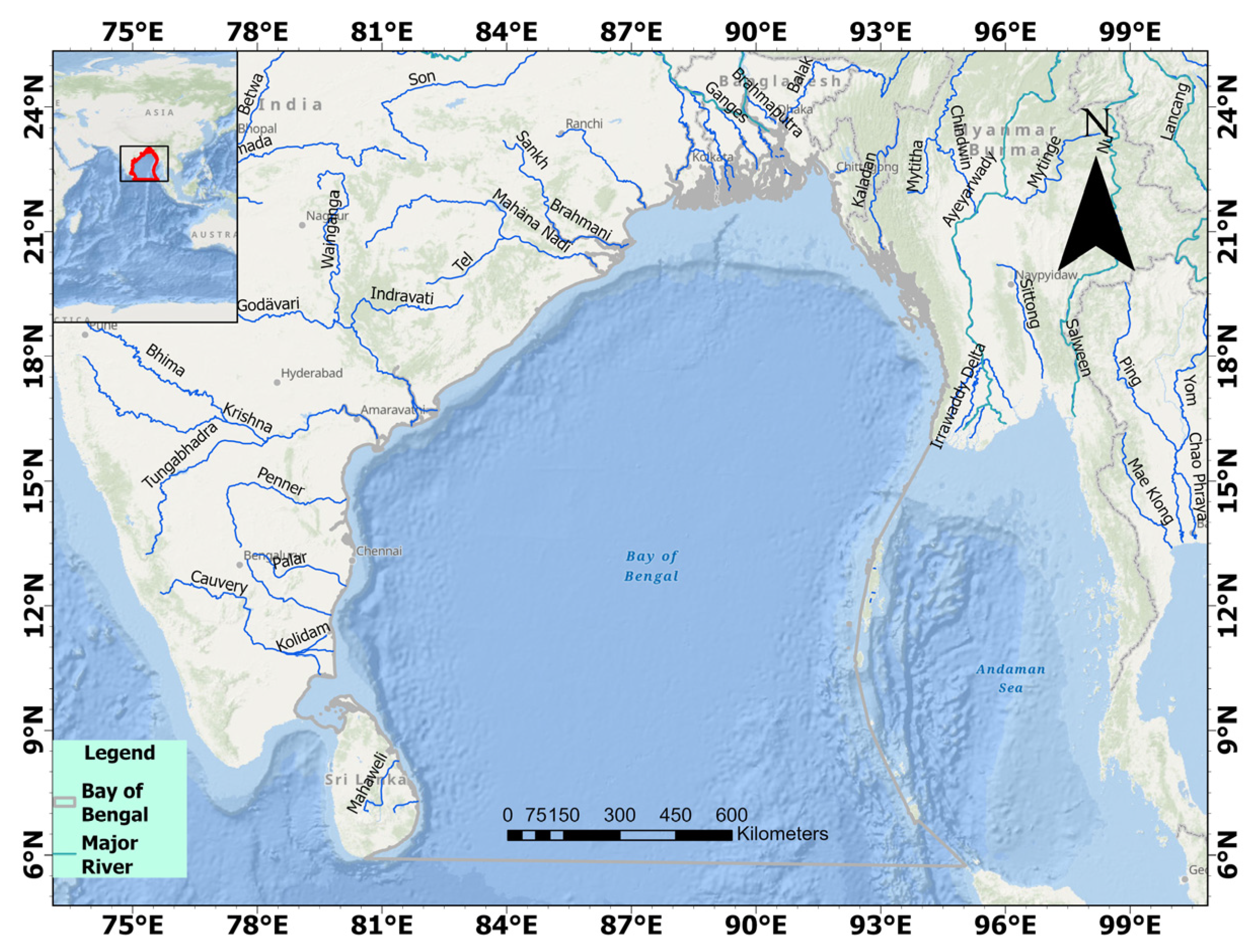
Figure 2.
Distribution of mesoscale eddies in the Bay of Bengal; A) anticyclonic eddies, B) cyclonic eddies, C) compilation of all eddies, and D) ratio of cyclonic to anticyclonic eddies.
Figure 2.
Distribution of mesoscale eddies in the Bay of Bengal; A) anticyclonic eddies, B) cyclonic eddies, C) compilation of all eddies, and D) ratio of cyclonic to anticyclonic eddies.
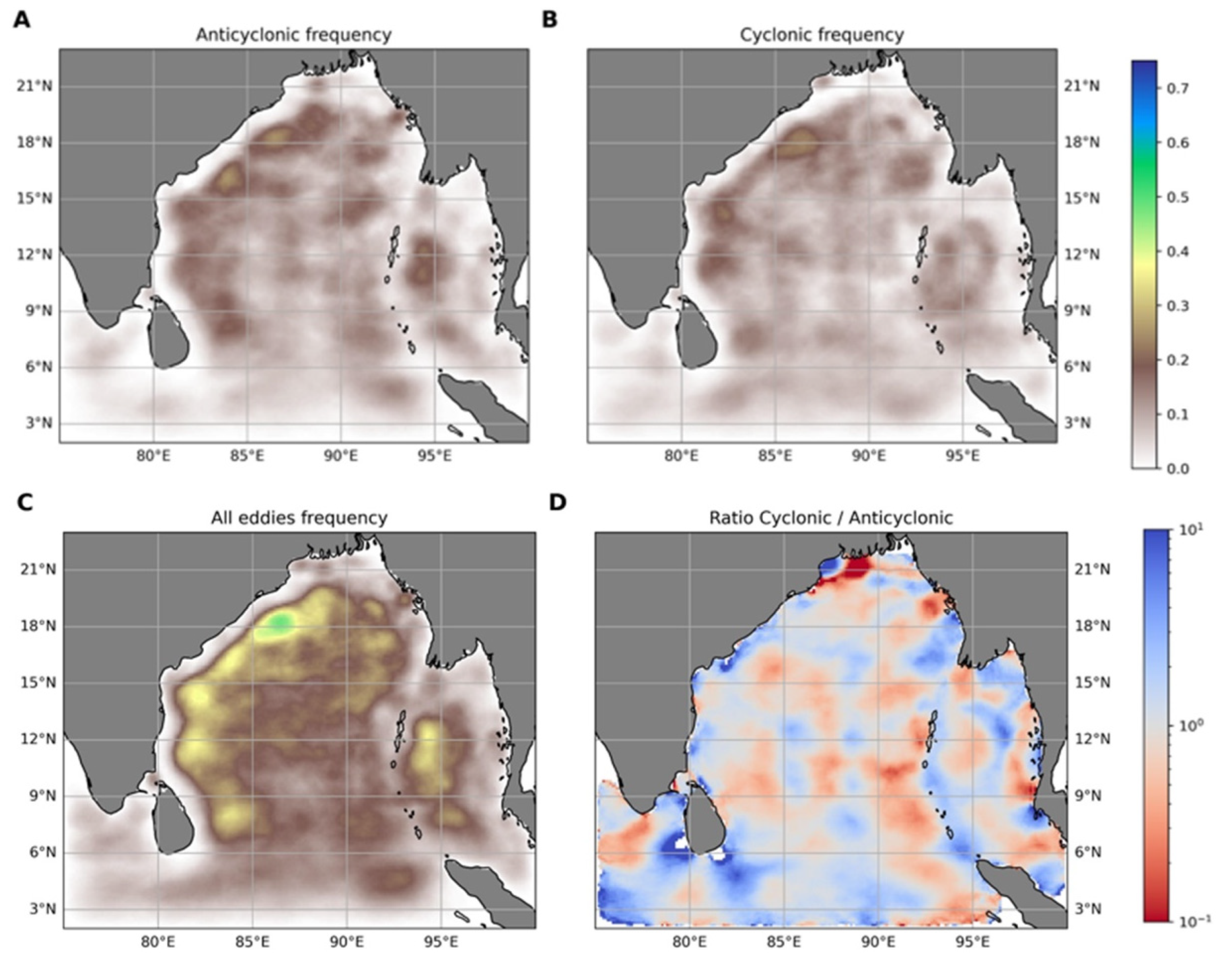
Figure 3.
Tracks of mesoscale eddies with varying lifespans. Subplots A-F correspond to eddies lasting from 1 week to 2 weeks and 5 or more weeks, encompassing both cyclonic and anticyclonic types.
Figure 3.
Tracks of mesoscale eddies with varying lifespans. Subplots A-F correspond to eddies lasting from 1 week to 2 weeks and 5 or more weeks, encompassing both cyclonic and anticyclonic types.
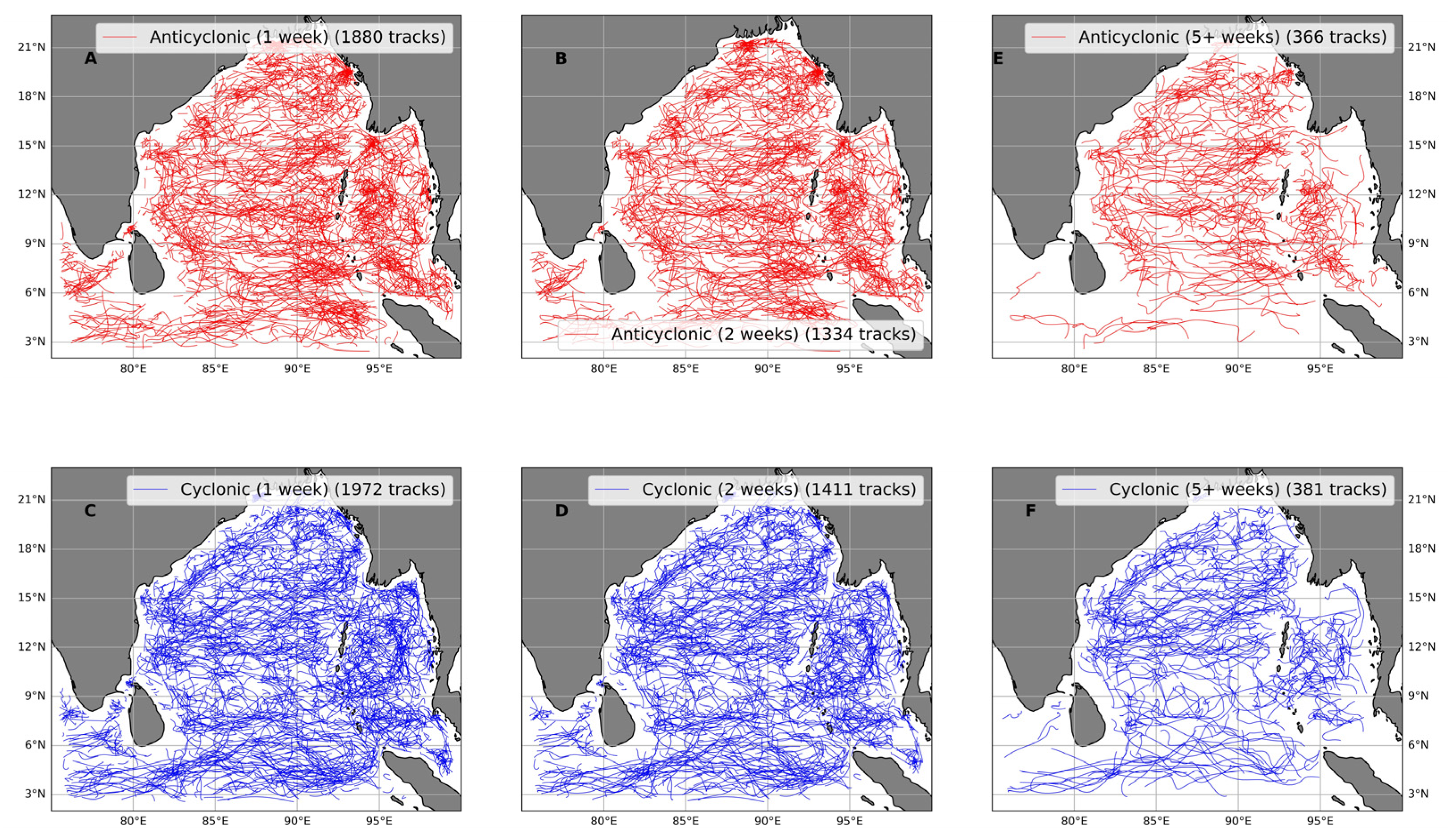
Figure 4.
Birth frequencies of cyclonic (A) and anticyclonic eddies (B).

Figure 5.
Eddy characteristics observed from the BoB, including A) Lifetime histogram, B) Number of eddies by year, C) cumulative number of eddies by year, D) ratio of cyclonic to anticyclonic eddies, and D) cumulative ratio of cyclonic to anticyclonic eddies. “Number of eddies by year” shows the yearly count, while the “Cumulative number of eddies by year” shows the total count from the starting year up to each subsequent year.

Figure 6.
Results from eddy propagation analysis; A) Number of eddies by year, B) cumulative number of eddies by year, C) ratio of cyclonic to anticyclonic eddies, and D) cumulative ratio of cyclonic to anticyclonic eddies.
Figure 6.
Results from eddy propagation analysis; A) Number of eddies by year, B) cumulative number of eddies by year, C) ratio of cyclonic to anticyclonic eddies, and D) cumulative ratio of cyclonic to anticyclonic eddies.

Figure 7.
Mesoscale eddy characteristics, Parameter Histogram; First column focuses on the amplitude of eddies in centimeters. Top plot (A1): Presents the cumulative percent distribution of the amplitude values. Middle plot (A2): Displays the histogram showing the percentage of observations for different amplitude values, Anticyclonic eddies are represented in red, and cyclonic eddies are represented in blue. Bottom plot (A3): Shows the ratio of the percentage of cyclonic to anticyclonic observations across different amplitude values. This ratio plot highlights the relative frequency of cyclonic versus anticyclonic eddies at each amplitude level. Second column (B): Indicates the speed radius in kilometers. The speed radius, also known as the eddies’ radius 𝑅max (it is the radius of the best-fit circle that matches the contour of the maximum circum-average geostrophic speed of the eddy). Top plot (B1): Displays the percentage of observations for different speed radius values. Middle plot (B2): Shows the cumulative percent distribution of the speed radius. Bottom plot (B3): Presents the ratio of cyclonic to anticyclonic observations for different speed radius values. Third column (C): Shows the average speed in centimeters per second. Top plot (C1): Displays the percentage of observations for different average speed values. Middle plot (C2): Shows the cumulative percent distribution of the average speed. Bottom plot (C3): Presents the ratio of cyclonic to anticyclonic observations for different average speed values.
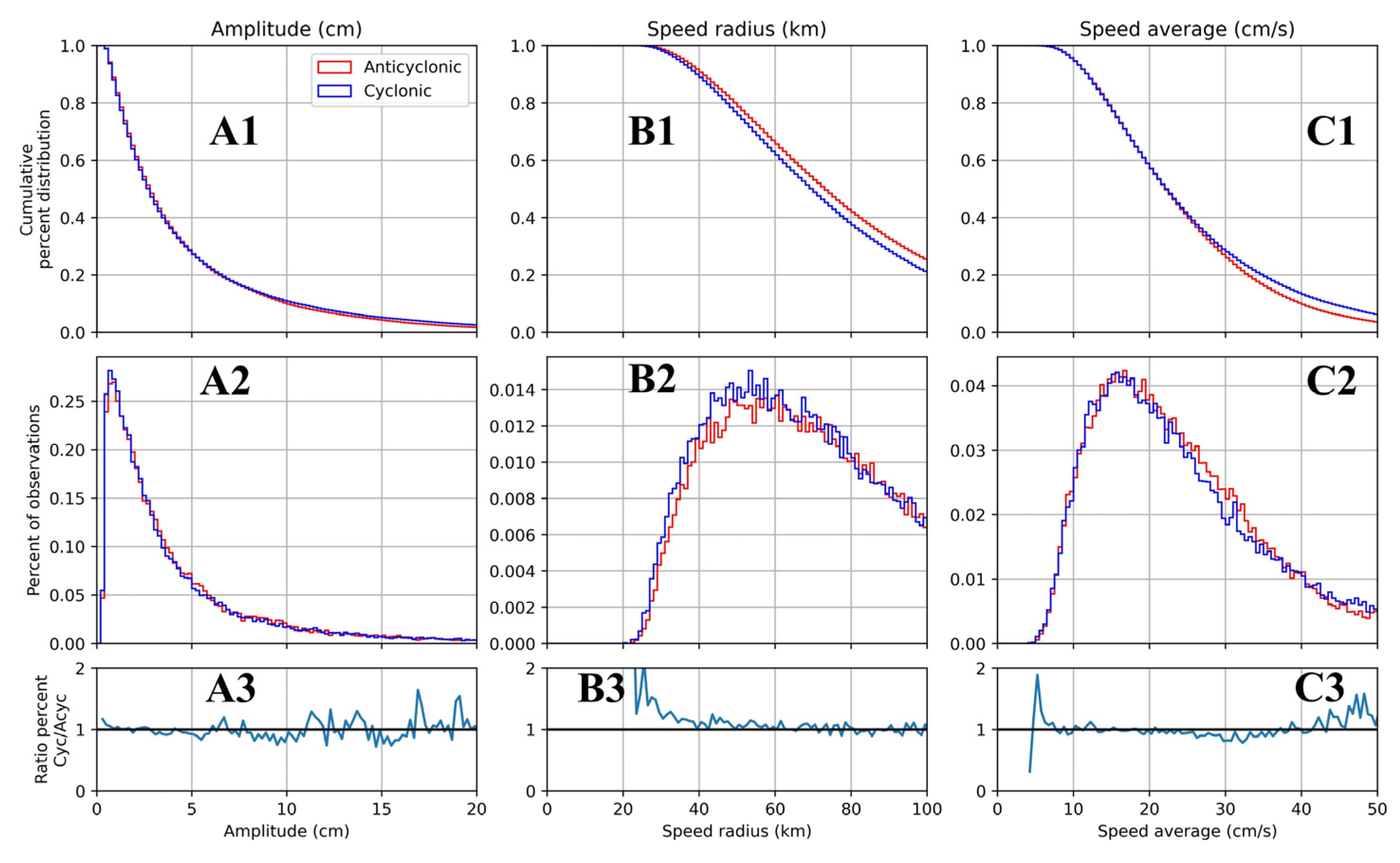
Figure 8.
Monsoon dominated seasonal surface geostrophic current (ms-1) distribution in the BoB; A) pre-monsoon season (March to May), B) southwest monsoon season (June to September), and C) northeast monsoon season (October to December).
Figure 8.
Monsoon dominated seasonal surface geostrophic current (ms-1) distribution in the BoB; A) pre-monsoon season (March to May), B) southwest monsoon season (June to September), and C) northeast monsoon season (October to December).
Disclaimer/Publisher’s Note: The statements, opinions and data contained in all publications are solely those of the individual author(s) and contributor(s) and not of MDPI and/or the editor(s). MDPI and/or the editor(s) disclaim responsibility for any injury to people or property resulting from any ideas, methods, instructions or products referred to in the content. |
© 2024 by the authors. Licensee MDPI, Basel, Switzerland. This article is an open access article distributed under the terms and conditions of the Creative Commons Attribution (CC BY) license (http://creativecommons.org/licenses/by/4.0/).
Copyright: This open access article is published under a Creative Commons CC BY 4.0 license, which permit the free download, distribution, and reuse, provided that the author and preprint are cited in any reuse.


