
Submitted:
13 June 2023
Posted:
14 June 2023
You are already at the latest version
Abstract
The Kuroshio Extension(KE) System exhibits highly energetic mesoscale phenomena, but the impact of mesoscale eddies on marine ecosystems and biogeochemical cycling is not well understood. This study utilizes remote sensing and Argo floats to investigate how eddies modify surface and subsurface chlorophyll (Chl-a) concentrations. On average, cyclones (anticyclones) induce positive (negative) surface Chl-a anomalies, particularly in winter. This occurs because cyclones (anticyclones) lift (deepen) isopycnals and nitrate into (out of) the euphotic zone, stimulating (depressing) the growth of phytoplankton. Consequently, cyclones (anticyclones) result in greater (smaller) subsurface Chl-a maximum (SCM), depth-integrated Chl-a, and depth-integrated nitrate. The positive (negative) surface Chl-a anomalies induced by cyclones (anticyclones) are mainly located near (north of) the main axis of the KE. The second and third mode represent monopole Chl-a patterns within eddy centers corresponding to either positive or negative anomalies, depending on the sign of the principal component. Chl-a concentrations in cyclones (anticyclones) above the SCM layer are higher (lower) than the edge values, while those below are lower (higher), regardless of winter variations. The vertical distributions and displacements of Chl-a and SCM depth are associated with eddy pumping. In terms of frequency, negative (positive) Chl-a anomalies account for approximately 26% (18%) of the total cyclones (anticyclones) across all four seasons. The opposite phase suggests that nutrient supply resulting from stratification differences under convective mixing may contribute to negative (positive) Chl-a anomalies in cyclone (anticyclone) cores. Additionally, the opposite phase can also be attributed to eddy stirring, trapping high and low Chl-a, and/or eddy Ekman pumping. Based on OFES outputs, the seasonal variation of nitrate from winter to summer primarily depends on the effect of vertical mixing, indicating that convective mixing processes contribute to an increase (decrease) in nutrients during winter (summer) over the KE.
Keywords:
mesoscale eddies
; chlorophyll concentrations
; biogeochemical cycling
1. Introduction
Mesoscale eddies, which encompass spatial scales ranging from 10 to 100 kilometers and temporal scales from weeks to months, are significant drivers of complex interactions within the ocean, including its physics, biology, and biogeochemistry [1]. These eddies are commonly observed in west boundary currents and are characterized by strong vertical and horizontal currents. The Kuroshio Extension (KE), situated in the North Pacific Ocean, is a notable component of the western boundary current. It is distinguished by its elevated temperature, salinity, flow velocity, and noticeable ocean color [2].
The Kuroshio Extension (KE) region is renowned for its prominent ocean front and the highest eddy kinetic energy globally. This unique oceanic area is influenced by various factors, including topography, monsoons, and the western boundary current. These factors contribute to the manifestation of complex and dynamic characteristics observed in the eddies present within the KE [3]. Throughout the lifecycle of an eddy, from its formation to dissipation, it actively transports its internal water mass in a westward direction. This transport is facilitated by a range of physical processes, including eddy stirring, trapping, pumping, and eddy-wind Ekman pumping [4,5,6,7,8,9,10]. These processes play a crucial role in facilitating horizontal exchange and vertical transport of physical and chemical constituents, such as heat, salt, kinetic energy, nutrients, and phytoplankton. The physical and biological processes within eddies has a significant impact on the ecological environment of the upper ocean [11,12,13]. The widely accepted eddy pumping process, based on satellite measurements of cyclonic (anticyclonic) eddies, suggests that the uplifting (deepening) of isopycnals and nitrate into (out of) the euphotic zone stimulates (inhibits) phytoplankton growth, resulting in elevated (reduced) concentrations of chlorophyll-a (Chl-a) [14,15,16,17,18,19,20]. With the advancement of Argo and Bio-Argo float deployments, researchers now have effective tools to explore the subsurface dynamics within eddies without relying solely on satellite observations. In a more recent study, Dufois et al. [8] conducted cruise observations and provided evidence that anticyclonic eddies in subtropical gyres exhibit intensified surface Chl-a concentrations during winter, attributed to convective mixing stirring the subsurface Chl-a maximum. Wang et al. [9] proposed that winter cyclonic eddies (CE) promote enhanced vertical blooms dominated by phytoplankton biomass due to shallow mixed layers and uplifted thermoclines.
In South China Sea, He et al. [10] found that intense downwelling within anticyclone eddies (ACE) leads to a substantially deeper and less pronounced subsurface Chl-a maximum compared to CE during summer. In the North Subtropical Pacific, Huang et al. [12] conducted studies and observed that the depth-integrated nitrate and Chl-a anomalies within eddies are generally within ±90% for nitrate and ±10% for Chl-a in the euphotic layer. However, it is worth noting that the magnitudes of these anomalies can vary significantly depending on individual eddy analyses. Rii et al. [21] and Bidigare et al. [22] reported substantial increases in anomalies within CE compared to areas outside of eddies, with magnitudes ranging from 3.3 to 9.0 times and 1.0 to 1.5 times, respectively. These variations highlight the importance of incorporating a significant amount of subsurface observation data to distinguish the contributions of different physical processes. Overall, Previous studies have provided valuable observational evidence concerning regional variations in the biogeochemical response to eddies. Nevertheless, the biogeochemical response driven by eddies remains unclear, particularly with regard to different seasons.
This study examines the seasonal variations in eddy-driven biogeochemical responses in the KE using satellite data and decades of oceanographic observation data. Eddy-associated surface Chl-a anomalies spanning 21 years are composited onto eddy-centric coordinates. Additionally, Argo floats are used to normalize Chl-a, nutrient, temperature, and salinity measurements into a standardized vertical profile, allowing for a statistical analysis of the vertical structure ( physical and biological) of eddies in the KE under different seasons. OFES outputs is used to evaluated the contribution of mesoscale dynamics to nutrient transport.
2. Materials and Methods
2.1. In Situ Data
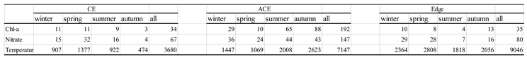
In situ data are obtained from global Argo project (Argo and Bio-Argo) (downloaded from http://www.argo.net), which are included the profile of temperature, salinity, Chl-a, nutrient and dissolved oxygen. The data are quality-controlled using automated procedures and assessed using statistical analysis residuals. Here, we extracted the in-situ data from 1998 to 2020 in thr KE to reveal the change of vertical physical and biochemical structures, approximately 19000 temperature and salinity profiles, 294 nitrate profiles, 261 Chl-a profiles (Table1). Argo floats (Chl-a, nutrient, temperature and salinity) are normalized into a standard vertical profile under different seasons,which provided a statistical view of the vertical structure(biological and physical) of eddied in the KE.

Table 1.
Numbers of Argo floats under different seasons.
2.2. Other data
The daily merged satellite product of Chl-a concentration data was obtained using a multisensor approach that integrated data from various sensors, such as SeaWiFS, MODIS, MERIS, VIIRS-SNPP, JPSS1, OLCI-S3A, and S3B. These algorithms were designed to provide accurate estimations with a spatial resolution of 4 km, catering to the needs of end-users. The Copernicus Marine Environmental Monitoring Center (CMEMS, http://marine.copernicus.eu/) served as the source for acquiring the data, which was utilized to analyze and characterize the biomass dynamics at the sea surface [23]. For the analysis of eddies, sea level anomaly (SLA) data were obtained from CMEMS. These data had a spatial resolution of 25 km and a temporal resolution of 1 day. Multimission altimetry datasets were used to detect the eddies. Each day, the detected eddies provided information on their location, type (cyclonic or anticyclonic), speed, radius, and associated metadata. The detection process employed a delayed-time algorithm (version DT2.0exp), which was developed and validated in collaboration with D. Chelton and M. Schlax at Oregon State University [1]. The altimetry period covered data from 1993 to the present. By utilizing these datasets and detection methods, the study aims to investigate the characteristics and behavior of eddies in the designated region.
The nutrient levels in the upper ocean, specifically above 200 m, were characterized by utilizing multi-year average profiles of nitrate. These profiles were derived from the World Ocean Atlas 2018 (WOA18), which can be accessed at https://www.nodc.noaa.gov/ocs/woa18
The OFES quasi-global eddy-resolving simulation (accessible at http://www.jamstec.go.jp/ofes/ofes.html) utilized the Modular Ocean Model ver.3 (MOM3), developed by GFDL/NOAA, with a horizontal resolution of 0.1 degree and 54 vertical levels featuring varying intervals from 5 m at the surface to 330 m at a maximum depth of 6065 m. By forcing the model with a 5-year integration of NCEP/NCAR monthly climatology, it successfully captured the annual cycle of temperature, nitrogen (the sole nutrient), and phytoplankton in the upper ocean [20]. These model outputs, encompassing variables such as velocity and nitrate, were employed in the present study to investigate the influence of mesoscale dynamics on biological production [9].
2.3. Composite analysis
In this study, the eddy trajectories product provided by Chelton et al. [1] covering the period from 1998 to 2021 was utilized. To analyze each eddy, the corresponding normalized Chl-a anomalies (Chl-a') field were collocated and projected onto a high-resolution grid with normalized eddy-centric coordinates. The grid used had a resolution of 0.025 and consisted of a 161x161 grid cells. The size of the collocation region was determined based on the eddy radius, denoted as R, ensuring accurate spatial alignment and analysis. Chl-a' were used for each composite individual eddy and calculated as:
Where , the overbar denotes the radial average and is the standard deviation, both computed over the eddy for r≤2R.
2.4. EOF analysis
Empirical Orthogonal Function (EOF) analysis was employed to identify dominant coherent variations and Chl-a' patterns within eddies across different seasons different seasons [24]. The space-time Chl-a data set A(x,y,t) can be expressed as:
Whereis the modulated function to show the corresponding temporal variation, and is the Kth model spatial patterns. Typically, the first three modes, characterized by higher variance, are likely to possess significant physical interpretations [25].
2.5. Mixed layer Nutrient Budget
To explore the influence of mesoscale dynamics on biological production, we examined the nitrate budget equation based on the formulation introduced by Caniaux and Planton [26] for the mixed layer heat budget. The rate of change of nitrate (N) within the mixed layer [27] is:
The formula consists of three terms on the right side, namely lateral advection, vertical advection, and vertical mixing. Using the Reynolds averaging method, the rate of change of N can be divided into contributions from the mean flow and the fluctuating eddy flow [28]:
where the overbar denotes a time mean to be defined and the prime all deviations from this time mean (referred as the eddy term).
3. Results
The study focused on the KE region, specifically the area between 30°N-40°N and 140°E-170°E, as illustrated in Figure 1. The standard deviation (STD) of the average SLA within this region, calculated from data spanning 1998 to 2020, exhibited high variability along the main axis of the KE at 35°N. Both the north and south sides of this axis displayed a substantial STD value of 0.3 m, indicative of pronounced eddy activity. The region adjacent to the main axis predominantly featured ACE on the north side and CE on the south side. Notably, the concentration of Chl-a within CE was significantly higher compared to ACE [11].
3.1. Eddy features
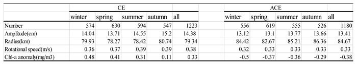
Table 2 presents the characteristics of eddies in the KE during different seasons from 1998 to 2020. The table includes information on the number, amplitude, and rotational speed of CE and ACE. The activity of both CE and ACE shows similar seasonal variations, with the highest activity observed in spring. While ACE generally have a larger radius across all seasons, CE exhibit slightly higher values in terms of number, average amplitude, and rotational speed compared to ACE. CE are characterized by their smaller size and greater intensity compared to ACE. Specifically, in winter, the number, amplitude, and rotational speed of CE are 3%, 7%, and 11% larger than those of ACE, respectively, while the radius of ACE is 13% smaller than that of CE. Additionally, we utilize a dimensionless coefficient (U/C, where U represents rotational speed and C denotes translational speed) greater than 1 to identify nonlinear eddies. This criterion indicates that the water within a certain depth maintains its distinct properties without exchanging with the surrounding environment [29]. Both CE and ACE exhibit a high level of nonlinearity according to this criterion [1].
Table 2.
Statistics of eddy properties in different seasons of KE.
 |
3.2. Eddy and Chl-a Relationship
The relationship between SLA and Chl-a concentrations in the KE region was investigated to gain insights into the impact of eddies on surface Chl-a levels. Figure 2 illustrates a notable negative correlation (r < 0.8, p < 0.05) between SLA and Chl-a, predominantly observed along the KE region (from 140 oE to 180 oE along 35 oE) throughout the four seasons. The areas exhibiting a significant correlation align with the regions of high SLA STD as depicted in Figure 1. These correlation patterns are in line with findings from previous studies [5,11]. The negative correlations can be attributed to the upwelling (downwelling) processes within CE (ACE), which transport nutrient-rich (poor) water from deeper (shallower) regions, respectively.
The spatial distribution of composite average normalized Chl-a concentrations across multiple eddies during different seasons provides detailed insights into the Chl-a response to CEs and ACEs (Figure 3). Monopole Chl-a patterns are observed only in winter and spring, indicating that higher (lower) Chl-a values within CEs (ACEs) during all four seasons correspond to positive (negative) Chl-a anomalies in the eddy center (r/R < 1) (Table 2). According to Table 2, the average Chl-a anomaly concentration in CEs (ACEs) is 0.48 (-0.5), 0.41 (-0.37), 0.31 (-0.36), and 0.11 (-0.29) mg/m3 during different seasons, respectively. These positive (negative) anomalies in CEs (ACEs) can be attributed to eddy pumping, which is associated with upwelling (downwelling) processes.
Additionally, the large-scale horizontal gradient of Chl-a plays a significant role in the spatial patterns observed across all four seasons. The meridional advection of Chl-a contributes to the generation of Chl-a anomalies along the edges of eddies [8], particularly during summer and autumn. Moreover, the clockwise (anticlockwise) rotation of eddy flows leads to the accumulation of Chl-a anomalies in the northwest (southeast) quadrant of the eddies, influenced by the water transport in eddy-centric coordinates.The EOF method was employed to decompose normalized Chl-a data across thousands of eddies into significant temporal and spatial components that capture the primary variability in the spatial patterns. Table 3 presents the variances of the first three temporal modes for different seasons, illustrating the significant spatial variability captured by the first three spatial EOF modes. Figure 4 and Figure 5 display these spatial EOF modes, which account for approximately 50% of the total variance in Chl-a for both CEs and ACEs. The first modes (variance: 18%~31%) correspond to the horizontal eddy stirring process, exhibiting Chl-a anomalies at the eddy edges. The second mode (variance: 12%~16%) represents monopole Chl-a patterns within the eddy centers, displaying either positive or negative anomalies based on the sign of the principal component. Moreover, most of the third mode (variance: 10%~14%) exhibits similarities to the second mode.
Figure 3 illustrates the composite averages of Chl-a anomalies associated with CEs and ACEs in the KE region. CEs exhibit positive Chl-a anomalies, while ACEs display negative Chl-a anomalies. However, it is important to note that not all eddies in the KE region exhibit Chl-a anomalies, as revealed by the EOF modes. Figure 4 and Figure 5 depict the variability in Chl-a values within CEs and ACEs, respectively. Similar patterns have been observed in subtropical gyres, where ACEs have been found to enhance Chl-a concentrations through the modulation of winter mixing by eddies, as suggested by Dufois et al. [8].
To calculate the Chl-a anomalies associated with CEs and ACEs, each eddy is individually assessed and mapped onto a 0.5°×0.5° grid. The results demonstrate that CEs generally increase Chl-a concentrations in most regions of the KE, while ACEs tend to decrease them. However, the magnitude of Chl-a anomalies varies across different regions. The spatial distribution of eddies also exhibits varying polarities. CEs induce higher positive Chl-a anomalies, primarily concentrated near the main axis of the KE. Conversely, negative anomalies are predominantly observed to the south of the main axis, while lower positive anomalies occur to the north. These negative anomalies account for 24% (winter), 23% (spring), 25% (summer), and 44% (autumn) of all CEs (Figure 6a-d-g-j). On the other hand, ACEs induce higher negative anomalies primarily north of the main axis, while positive anomalies are predominantly observed to the south. The positive anomalies account for 19% (winter), 21% (spring), 16% (summer), and 20% (autumn) of all ACEs (Figure 6b-e-h-k).
Previous research conducted by Itoh and Yasuda [30] has indicated that CEs are more commonly observed in the southern region of the KE compared to the northern region. This spatial distribution of eddies suggests that eddy activity may play a role in the regional variations observed in Chl-a anomalies associated with CEs and ACEs. Specifically, CEs located near the KE are more likely to encounter water with higher concentrations of Chl-a and nutrients originating from the northern region of the KE.
3.3. Vertical Profiles of Temperature, Chl-a and Nitrate in Eddies
We conducted an analysis of eddy trajectories [1] and the distribution of approximately 19,000 temperature and salinity profiles, 294 nitrate profiles, and 261 Chl-a profiles obtained from the Argo program in the KE region (refer to Table 1). Among these profiles, 3,680 (7,100) temperature/salinity profiles were associated with CEs (ACEs), while 34 (192) Chl-a profiles and 64 (147) nitrate profiles were observed in CEs (ACEs). The higher number of profiles in ACEs compared to CEs can be attributed to the larger size of ACEs, as indicated in Table 2. In addition, we identified 9,000 temperature/salinity profiles, 35 Chl-a profiles, and 140 nitrate profiles located at the edges of the eddies. To facilitate analysis, the Chl-a, nutrient, temperature, and salinity data from the Argo floats were normalized into standardized vertical profiles corresponding to different seasons (Figure 7, Figure 8 and Figure 9).
Figure 7 illustrates the temperature characteristics within the depth range of 0-300 m. It demonstrates that the temperature is lower (higher) in CEs (ACEs) than in ACEs (CEs) and at the eddy edges during all seasons. During the colder seasons (winter and spring), the average temperature ranges between 10-20 ℃. However, in the warmer seasons (summer and autumn), there is a noticeable increase of approximately 10 ℃ in the temperature within the 0-100 m depth range. The mixed layer depth (MLD) experiences different patterns in CEs and ACEs. The MLD deepens to 90 m (120 m) due to winter deep mixing in CEs (ACEs), while the MLD shoals to 10 m (20 m) in CEs (ACEs) owing to seasonal stratification in summer. The variations in MLD within the same season indicate the presence of upwelling and downwelling processes, which contribute to vertical fluctuations within eddies and influence the vertical flux of nutrients and Chl-a.
Figure 8 illustrates the vertical distribution of Chl-a within eddies. The results reveal that near-surface Chl-a concentrations are higher in CEs compared to the eddy edges, while ACEs exhibit lower near-surface Chl-a concentrations. This pattern is consistent with the variations observed in near-surface Chl-a from satellite data (Figure 3), except for autumn. Additionally, the depth of the subsurface Chl-a maximum (SCM) layer is shallower in CEs than in ACEs. Specifically, the SCM depths in CEs are 48 m (spring), 36 m (summer), 54 m (autumn), and 30 m (winter), while in ACEs, they are 75 m (spring), 81 m (summer), 78 m (autumn), and 35 m (winter). It is important to note that the vertical distribution of Chl-a above 100 m is relatively uniform due to winter mixing. The SCM within CEs reaches values of 0.87 mg/m3 (winter), 2.3 mg/m3 (spring), 1.5 mg/m3 (summer), and 0.91 mg/m3 (autumn), which are significantly higher compared to the edge values. In contrast, the SCM values in ACEs are 0.59 mg/m3 (winter), 0.82 mg/m3 (spring), 0.7 mg/m3 (summer), and 0.52 mg/m3 (autumn).
In general, the vertical distribution of Chl-a within eddies exhibits distinct patterns. Above the SCM layer, Chl-a concentrations are higher within CEs and lower within ACEs compared to the values at the eddy edges (Figures 8abcd). Conversely, below the SCM layer, Chl-a concentrations are lower within CEs and higher within ACEs than the edge values (Figures 8bcd), regardless of seasonal variations. These vertical distributions and displacements of Chl-a and SCM depth are associated with upwelling in CEs and downwelling in ACEs. These observations are consistent with the enrichment of nutrients within CEs and the depletion of nutrients within ACEs (Figure 9).
The depth-integrated nitrate over the upper 150 m is higher within CEs and lower within ACEs compared to the edge values in each season. Specifically, it is 13% (winter), 25% (spring), 50% (summer), and 7% (autumn) higher within CEs, and 23% (winter), 37% (spring), 50% (summer), and 20% (autumn) lower within ACEs. Furthermore, the depth-integrated Chl-a is higher within CEs and lower within ACEs compared to the edge values. It is 25% (winter), 42% (spring), 90% (summer), and 13% (autumn) higher within CEs, and 9% (winter), 19% (spring), 5% (summer), and 24% (autumn) lower within ACEs. These variations can be attributed to the vertical movement of isopycnals and nitrate, resulting in the stimulation or depression of phytoplankton growth and thus affecting the depth-integrated Chl-a within CEs and ACEs. However, due to rapid biological removal processes within the euphotic layer (40-60 m), significant variations in nitrate concentration associated with high Chl-a within the SCM layer are challenging to observe [12,31,32].
In winter, despite high nutrient levels, reduced light availability limits a substantial increase in depth-integrated Chl-a within eddies. Therefore, changes in the vertical distribution of Chl-a during winter result from the redistribution of preexisting Chl-a through enhanced vertical mixing. The higher depth-integrated Chl-a during the spring bloom can be explained by various hypotheses, including the critical depth, shoaling mixing layer, critical turbulence, onset of stratification, and disturbance-recovery hypotheses. In summer, the depth-integrated Chl-a decreases but remains higher than in autumn. This is attributed to high light availability and the influence of mesoscale modulation of the mixed layer depth on the persistence of high Chl-a/nitrate concentrations originating from the spring period, resulting in a more prominent SCM than in autumn [33]. Overall, these findings demonstrate that the relationship between Chl-a and nutrients undergoes seasonal variations, reflecting alternating limiting factors and nitrate availability for primary production.
4. Discussion
In this study, we have observed that CEs in the KE region exhibit higher surface Chl-a concentrations compared to the edge values, while ACEs show lower surface Chl-a concentrations. This pattern is particularly pronounced during the cold seasons (winter and spring) when Chl-a levels are typically at their highest. The analysis of Chl-a patterns within eddies, using EOF analysis, has revealed the complexity of these relationships, indicating that multiple mechanisms contribute to the interaction between eddies and Chl-a dynamics.
Nutrients and light availability are crucial factors influencing phytoplankton blooms. Eddies play a significant role in shaping the vertical distribution of Chl-a and nitrate through processes such as eddy pumping, eddy Ekman pumping, eddy stirring, variations in light conditions, and vertical mixing, which vary across different seasons [12,16,34]. The modulation of the MLD by eddies has also been identified as a contributing factor to elevated Chl-a levels [8,18]. In our study, we followed the approaches of previous researchers [16,35] to investigate how MLD within eddies affects the distribution of Chl-a and nitrate. Despite the seasonal variation in our data, the integrated Chl-a (I-Chl), SCM, and deep SCM (DSCM) showed significant correlations with SLA (r = -0.58, -0.38, -0.27; Figure 10), all with p < 0.01. Similarly, integrated nitrate (I-nitrate) exhibited a strong negative correlation (r = -0.47, p < 0.01) with SLA (Figure 12a). These findings indicate that I-Chl, SCM, DSCM, and I-nitrate are more pronounced within CEs compared to the eddy edges, but weaker within ACEs. Furthermore, Figure 12 and Figure 13b demonstrate a significant correlation between I-Chl, SCM, DSCM, I-nitrate, and MLD (r = 0.45, -0.33, -0.21, 0.19; Figure 11 and 12b), all with p < 0.01. Deeper MLD corresponds to decreased SCM and DSCM by factors of 0.005 mg/m4 and 0.1765 m, respectively. Conversely, I-Chl and I-nitrate increase linearly by factors of 0.29 mg/m4 and 0.75 μmol/L/m, respectively, with MLD deepening. Notably, most CEs (blue marks) exhibit larger SCM, DSCM, I-Chl, and I-nitrate values compared to ACEs (pink marks). Previous studies have demonstrated that CEs are associated with shallower euphotic depths than ACEs, providing more favorable light conditions for phytoplankton growth and leading to larger SCM and I-Chl values [14,15,16,36]. These findings highlight the critical role of nutrient supply in driving phytoplankton blooms.
The modulation of MLD within eddies plays a significant role in shaping the distribution of Chl-a. Generally, CEs (ACEs) enhance (dampen) nutrient supply through eddy-induced upwelling (downwelling), leading to high (low) Chl-a concentrations [5]. Previous studies have shown that eddy pumping is the dominant mechanism controlling the biogeochemical response in eddies, resulting in upward and downward displacement of the SCM layer [12]. However, other studies propose that ACEs are more productive than CEs in subtropical gyres due to winter deeper mixing (MLD), which enhances nutrient supply to the mixed layer and/or redistributes Chl-a through stirring of the SCM [7,8,18]. In summer, the shallow MLD without strong vertical mixing does not promote the stirring of the SCM [16]. Figure 13 illustrates that changes in the MLD are influenced by turbulent vertical mixing and adiabatic processes associated with vertical stretching and/or eddy pumping [18]. Eddy pumping leads to a deeper MLD in ACEs compared to CEs throughout the year, with the most significant differences observed in winter. Both ACEs and CEs exhibit a shallow mixed layer with stable water (stronger N2) throughout the year (Figure 13a and b). From summer to winter, as the mixed layer deepens, the shallow stratification dissipates, and the nitrate flux peaks by the end of winter. Subsequently, the water column undergoes restratification starting from spring. In CE (ACE), the summer stratification is stronger (weaker) than that in ACE (CE), resulting in a shallower (deeper) MLD, which facilitates a greater (smaller) injection of nutrients into the mixed layer during winter (Figure 13). However, these changes in MLD do not align with the occurrence of higher (lower) average Chl-a concentrations in CEs (ACEs). It is worth noting that negative (positive) Chl-a values in the core of CEs (ACEs) account for a significant proportion of the total CEs (ACEs) during winter (24% and 19%, respectively). This suggests that the differences in stratification during winter convective mixing, leading to variations in nutrient supply, may contribute to negative (positive) Chl-a concentrations in the core of CEs (ACEs). The opposite Chl-a phase can also be attributed to eddy stirring, which traps areas of high and low Chl-a concentrations, and/or eddy Ekman pumping [37].
Additionally, it is important to consider the influence of submesoscale processes in the KE system, which are most pronounced during winter and spring [38]. Submesoscale features exhibit higher vertical velocities compared to eddies [39], making them important contributors to phytoplankton production by transporting nutrients and phytoplankton into the sunlit ocean [40,41,42]. This transport mechanism plays a significant role in promoting phytoplankton production. Although the analysis in this study may not fully capture the submesoscale features due to the spatial resolution of the data and potential obscuration in the EOF patterns, it is essential to acknowledge their potential influence for a comprehensive understanding of the biogeochemical dynamics in the KE system.
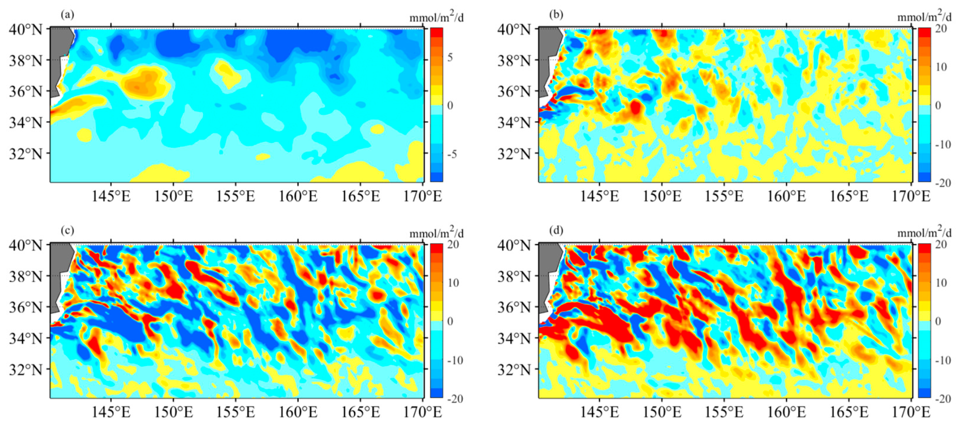
To assess the influence of mesoscale dynamics on biological production, the mixed-layer nitrogen budget is analyzed using the OFES hydrography-biology products [9,28]. The nitrogen change in the OFES model (in mmol m-2 d-1) is divided into three components: mean advective flow, eddy flow, and mixing. During winter, the average nitrate increase is 2.67, with the three components contributing as follows: 0.54 (mean advective flow), -5.13 (eddy flow), and 7.26 (mixing) (Figure 14). In contrast, summer exhibits an average nitrate decrease of 4.64, with the three components contributing as follows: -0.34 (mean advective flow), -5.93 (eddy flow), and 1.64 (mixing) (Figure 15). These results indicate that eddy flows play a significant role in nutrient depletion, while the mean flow has a relatively minor impact and contributes minimally to nutrient changes. The magnitude of these flows does not exhibit clear seasonal variation. On the other hand, the mixing component displays substantial variations in magnitude. Therefore, the seasonal variation of nitrate primarily depends on the influence of vertical mixing, highlighting the contribution of convective mixing processes to nutrient increase (winter) or decrease (summer) in the KE region.
5. Conclusions
This study investigates the influence of mesoscale and submesoscale processes on biological production in the KE System. Using remote sensing and Argo floats, the researchers explore how eddies modify surface and subsurface Chl-a concentrations. CE and ACE induce positive and negative surface Chl-a anomalies, respectively, particularly in winter. This is due to the lifting or deepening of isopycnals and nitrate, stimulating or depressing phytoplankton growth. Consequently, CE and ACE result in variations in SCM depth-integrated Chl-a, and nitrate. These anomalies are mainly located near the main axis of the KE. Monopole Chl-a patterns within eddy centers correspond to positive or negative anomalies, depending on the principal component's sign. Chl-a concentrations above the SCM layer in CE and ACE are higher and lower than the edge values, respectively, while those below exhibit the opposite pattern, regardless of winter variations. Negative and positive Chl-a anomalies account for approximately 26% and 18% of the total CE and ACE, respectively, across all seasons. Nutrient supply resulting from stratification differences under convective mixing and eddy stirring may contribute to these anomalies. The study also highlights the role of submesoscale processes, such as higher vertical velocity in winter and spring, in transporting nutrients and phytoplankton into the sunlit ocean and promoting significant phytoplankton production. However, the study acknowledges the need for improved spatial resolution and comprehensive observations to fully understand submesoscale processes. Another study examined MLD adjustment in eddies, revealing the influence of eddy-induced upwelling and downwelling in CE and ACE on nutrient supply and Chl-a concentrations. The differences between CE and ACE are more significant in winter due to deeper mixing, enhanced nutrient supply, and redistribution of Chl-a. The shallow mixed layer and stratification in summer affect nutrient injection and contribute to variations in Chl-a concentrations. Convective mixing processes also play a role in nutrient increase or decrease during winter and summer, respectively. Overall, this study highlights the importance of mesoscale and submesoscale processes in driving biological productivity in the KE system.
Overall, the study emphasizes the importance of mesoscale and submesoscale processes in driving biological productivity and provides insights into the mechanisms underlying nutrient supply and Chl-a distributions in the KE system. While shedding light on these dynamics, the study acknowledges the need for future research to improve spatial resolution and incorporate comprehensive observations for a better understanding of submesoscale features and their impacts.
Author Contributions
T.W. and S.Z. conceived and designed the study. T.W. helped with writing and provided thorough editing. T.W. and F.C. contributed to the writing and data interpretation. Data analyses were conducted mainly by T.W. and L.X. All authors have read and agreed to the published version of the manuscript.
Funding
This research was funded by Lingnan Normal University, grant number 000302302637.
Acknowledgments
The authors would like to thank the anonymous reviewers and editor for their very constructive comments. The comments and suggestions provided by the reviewers and editor have greatly enhanced the quality and presentation of this work. The authors would also like to extend their thanks to the Copernicus Marine Environmental Monitoring Center (CMEMS), the global Argo project, the National Oceanic and Atmospheric Administration (NOAA), the Japan Agency for Marine-Earth Science and Technology (JAMSTEC) scientific teams, as well as D. Chelton and M. Schlax for their contributions in processing and providing the essential datasets used in this study.
Conflicts of Interest
The authors declare no conflict of interest.
References
- Chelton D B, Schlax M G, Samelson R M. Global observations of nonlinear mesoscale eddies. Progress in oceanography, 2011, 91(2): 167-216. [CrossRef]
- Qiu, B. Kuroshio Extension variability and forcing of the Pacific decadal oscillations: Responses and potential feedback. Journal of Physical Oceanography, 2003, 33(12): 2465-2482. [CrossRef]
- Qiu, B. , & Chen, S. Variability of the Kuroshio Extension jet, recirculation gyre, and mesoscale eddies on decadal time scales. Journal of Physical Oceanography, 2005, 35(11): 2090-2103. [CrossRef]
- Siegel, D. A. , Peterson, P., McGillicuddy Jr, D. J., Maritorena, S., & Nelson, N. B. Bio-optical footprints created by mesoscale eddies in the Sargasso Sea. Geophysical Research Letters, 2011, 38(13). [CrossRef]
- Gaube, P. , Chelton, D. B., Strutton, P. G., & Behrenfeld, M. J. Satellite observations of chlorophyll, phytoplankton biomass, and Ekman pumping in nonlinear mesoscale eddies. Journal of Geophysical Research: Oceans, 2013, 118(12): 6349-6370. [CrossRef]
- Jose, Y. S. , Aumont, O., Machu, E., Penven, P., Moloney, C. L., & Maury, O. Influence of mesoscale eddies on biological production in the Mozambique Channel: Several contrasted examples from a coupled ocean-biogeochemistry model. Deep Sea Research Part II: Topical Studies in Oceanography, 2014, 100: 79-93. [CrossRef]
- Dufois, F. , Hardman-Mountford, N. J., Fernandes, M., Wojtasiewicz, B., Shenoy, D., Slawinski, D.,... & Toresen, R. Observational insights into chlorophyll distributions of subtropical South Indian Ocean eddies. Geophysical Research Letters, 2017, 44(7): 3255-3264. [CrossRef]
- Dufois, F. , Hardman-Mountford, N. J., Greenwood, J., Richardson, A. J., Feng, M., & Matear, R. J. Anticyclonic eddies are more productive than cyclonic eddies in subtropical gyres because of winter mixing. Science advances, 2016, 2(5): e1600282. [CrossRef]
- Wang, T. , Du, Y., Liao, X., & Xiang, C. Evidence of eddy-enhanced winter chlorophyll-a blooms in northern Arabian Sea: 2017 cruise expedition. Journal of Geophysical Research: Oceans, 2020, 125(4): e2019JC015582. [CrossRef]
- He, Q. , Zhan, H., Xu, J., Cai, S., Zhan, W., Zhou, L., & Zha, G. Eddy-induced chlorophyll anomalies in the western South China Sea. Journal of Geophysical Research: Oceans, 2019, 124(12): 9487-9506. [CrossRef]
- Kouketsu, S. , Kaneko, H., Okunishi, T., Sasaoka, K., Itoh, S., Inoue, R., & Ueno, H. Mesoscale eddy effects on temporal variability of surface chlorophyll a in the Kuroshio Extension. Journal of Oceanography, 2016, 72: 439-451. [CrossRef]
- Huang, J. ,&Xu F. Observational evidence of subsurface chlorophyll response to mesoscale eddies in the North Pacific. Geophysical Research Letters, 2018, 45(16): 8462-8470. [CrossRef]
- Siswanto, E. , Sasai, Y., Matsumoto, K., & Honda, M. C. Winter–Spring Phytoplankton Phenology Associated with the Kuroshio Extension Instability. Remote Sensing, 2022, 14(5): 1186. [CrossRef]
- McGillicuddy Jr D J, Robinson A R. Eddy-induced nutrient supply and new production in the Sargasso Sea. Deep Sea Research Part I: Oceanographic Research Papers, 1997, 44(8): 1427-1450. [CrossRef]
- McGillicuddy Jr, D. J. , Robinson, A. R., Siegel, D. A., Jannasch, H. W., Johnson, R., Dickey, T. D.,... & Knap, A. H. Influence of mesoscale eddies on new production in the Sargasso Sea. Nature, 1998, 394(6690): 263-266. [CrossRef]
- He, Q. , Zhan, H., Cai, S., & Zha, G. On the asymmetry of eddy-induced surface chlorophyll anomalies in the southeastern Pacific: The role of eddy-Ekman pumping. Progress in Oceanography, 2016, 141: 202-211. [CrossRef]
- Wang, T. , Chen, F., Zhang, S., Pan, J., Devlin, A. T., Ning, H., & Zeng, W. Remote Sensing and Argo Float Observations Reveal Physical Processes Initiating a Winter-Spring Phytoplankton Bloom South of the Kuroshio Current Near Shikoku. Remote Sensing, 2020, 12(24): 4065. [CrossRef]
- Dufois, F. , Hardman-Mountford, N. J., Greenwood, J., Richardson, A. J., Feng, M., Herbette, S., & Matear, R. Impact of eddies on surface chlorophyll in the South Indian Ocean. Journal of Geophysical Research: Oceans, 2014, 119(11): 8061-8077. [CrossRef]
- Huang, J. , Xu, F., Zhou, K., Xiu, P., & Lin, Y. Temporal evolution of near-surface chlorophyll over cyclonic eddy lifecycles in the southeastern Pacific. Journal of Geophysical Research: Oceans, 2017, 122(8): 6165-6179. [CrossRef]
- Sasai, Y. , Sasaoka, K., Sasaki, H., & Ishida, A. Seasonal and intra-seasonal variability of chlorophyll-a in the North Pacific: model and satellite data. Journal of the Earth Simulator, 2007, 8(11): 3-11. [CrossRef]
- Rii, Y. M. , Brown, S. L., Nencioli, F., Kuwahara, V., Dickey, T., Karl, D. M., & Bidigare, R. R. The transient oasis: Nutrient-phytoplankton dynamics and particle export in Hawaiian lee cyclones. Deep Sea Research Part II: Topical Studies in Oceanography, 2008, 55(10-13): 1275-1290. [CrossRef]
- Bidigare, R. R. , Benitez-Nelson, C., Leonard, C. L., Quay, P. D., Parsons, M. L., Foley, D. G., & Seki, M. P. Influence of a cyclonic eddy on microheterotroph biomass and carbon export in the lee of Hawaii. Geophysical Research Letters, 2003, 30(6). [CrossRef]
- Maritorena, S. , d'Andon, O. H. F., Mangin, A., & Siegel, D. A. Merged satellite ocean color data products using a bio-optical model: Characteristics, benefits and issues. Remote Sensing of Environment, 2010, 114(8): 1791-1804. [CrossRef]
- Kaihatu, J. M. , Handler, R. A., Marmorino, G. O., & Shay, L. K. Empirical orthogonal function analysis of ocean surface currents using complex and real-vector methods. Journal of atmospheric and oceanic technology, 1998, 15(4): 927-941. [CrossRef]
- Lorenz, E. N. Empirical orthogonal functions and statistical weather prediction (Vol. 1, p. 52). Cambridge: Massachusetts Institute of Technology, Department of Meteorology. 1956.
- Caniaux, G. , & Planton, S. (1998). A three-dimensional ocean mesoscale simulation using data from the SEMAPHORE experiment: Mixed layer heat budget. Journal of Geophysical Research: Oceans, 1998, 103(C11): 25081-25099. [CrossRef]
- Radenac, M. H. , Jouanno, J., Tchamabi, C. C., Awo, M., Bourlès, B., Arnault, S., & Aumont, O. Physical driversof the nitrate seasonal variability in the Atlantic cold tongue. Biogeosciences, 2020, 17(2): 529-545. [CrossRef]
- Resplandy, L. , Lévy, M., Madec, G., Pous, S., Aumont, O., & Kumar, D. Contribution of mesoscale processes to nutrient budgets in the Arabian Sea. Journal of Geophysical Research: Oceans, 2011, 116(C11). [CrossRef]
- Flierl, G. R. Particle motions in large-amplitude wave fields. Geophysical & Astrophysical Fluid Dynamics, 1981, 18(1-2): 39-74. [CrossRef]
- Itoh, S. , & Yasuda, I. Characteristics of mesoscale eddies in the Kuroshio–Oyashio Extension region detected from the distribution of the sea surface height anomaly. Journal of Physical Oceanography, 2010, 40(5): 1018-1034. [CrossRef]
- Karl, D. M. , & Church, M. J. Microbial oceanography and the Hawaii Ocean Time-series programme. Nature Reviews Microbiology, 2014, 12(10), 699–713. [CrossRef]
- Karl, D. M. , & Church, M. J. Ecosystem structure and dynamics in the North Pacifific subtropical gyre: New views of an old ocean. Ecosystems, 2017, 20(3), 433–457. [CrossRef]
- Song, H. , Long, M. C., Gaube, P., Frenger, I., Marshall, J., & McGillicuddy, D. J. Seasonal variation in the correlation between anomalies of sea level and chlorophyll in the Antarctic Circumpolar Current. Geophysical Research Letters, 2018, 45, 5011–5019. [Google Scholar]
- Gao, W. , Wang, Z., & Zhang, K. Controlling effects of mesoscale eddies on thermohaline structure and in situ chlorophyll distribution in the western North Pacifific. Journal of Marine Systems, 2017, 175, 24–35. [Google Scholar] [CrossRef]
- Xiu, P. , & Chai, F. Eddies affect subsurface phytoplankton and oxygen distributions in the North Pacific Subtropical Gyre. Geophysical Research Letters, 2020, 47(15), e2020GL087037. [CrossRef]
- Oschlies, A. , & Garçon, V. Eddy-induced enhancement of primary production in a model of the North Atlantic Ocean. Nature, 1998, 394(6690), 266-269. [CrossRef]
- Chelton, D. B. , Gaube, P., Schlax, M. G., Early, J. J., & Samelson, R. M. The influence of nonlinear mesoscale eddies on near-surface oceanic chlorophyll. Science, 2011, 334(6054), 328-332. [CrossRef]
- Dong, J. , Fox-Kemper, B., Zhang, H., & Dong, C. The seasonality of submesoscale energy production, content, and cascade. Geophysical Research Letters, 2020, 47(6), e2020GL087388. [CrossRef]
- Ruiz, S. , Claret, M., Pascual, A., Olita, A., Troupin, C., Capet, A.,... & Mahadevan, A.Effects of oceanic mesoscale and submesoscale frontal processes on the vertical transport of phytoplankton. Journal of Geophysical Research: Oceans, 2019, 124(8): 5999-6014. [CrossRef]
- Uchida, T. , Balwada, D., Abernathey, R. P., McKinley, G. A., Smith, S. K., & Lévy, M. Vertical eddy iron fluxes support primary production in the open Southern Ocean. Nature Communications, 2020, 11(1): 1125. [CrossRef]
- Lévy, M. , Ferrari, R., Franks, P. J., Martin, A. P., & Rivière, P. Bringing physics to life at the submesoscale. Geophysical Research Letters, 2012, 39(14). [CrossRef]
- Zhang,Z.,&Qiu,B. Surface chlorophyll enhancement in mesoscale eddies by submesoscale spiral bands. Geophysical Research Letters, 2020, 47(14): e2020GL088820. [CrossRef]
Figure 1.
Spatial distribution of standard deviation for SLA from 1993 to 2020 year.
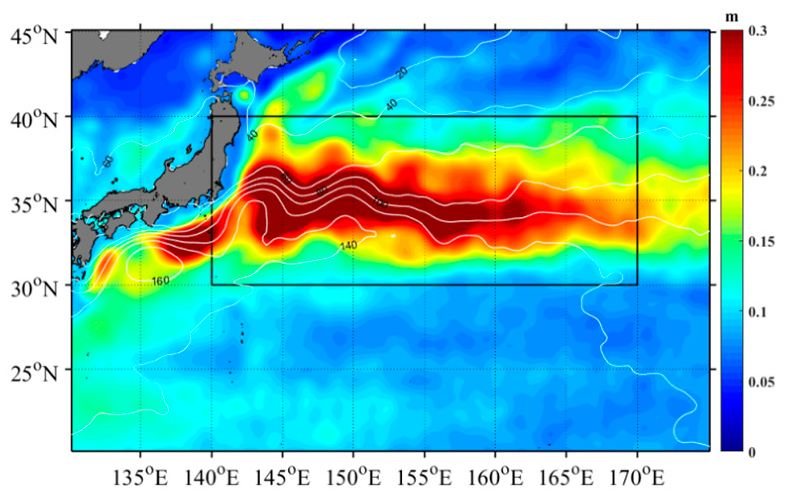
Figure 2.
Spatial distribution of correlation(a:winter; b:spring; c:summer; d:autumn) between SLA and Chl-a anomaly corresponding to eddies from 1993 to 2017. Plus sign denote significant correlations at a 95 % confidence level.
Figure 2.
Spatial distribution of correlation(a:winter; b:spring; c:summer; d:autumn) between SLA and Chl-a anomaly corresponding to eddies from 1993 to 2017. Plus sign denote significant correlations at a 95 % confidence level.
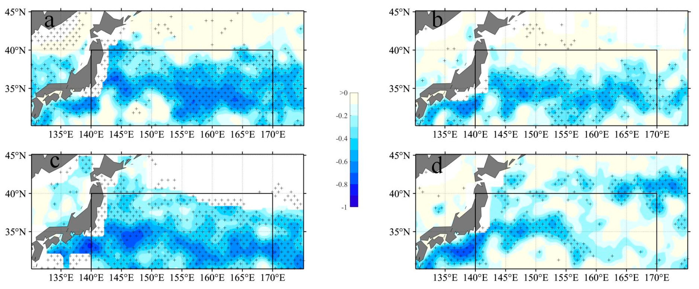
Figure 3.
Composite averages of winter (a and c), spring (b and f), summer (c and g) and autumn (d and h) Chl-a anomalies associated with Cyclonic and Anticyclonic eddy in the KE during the period 1998 to 2016. Inner and outer circles respectively coincide with r/R<1 and r/R<2.
Figure 3.
Composite averages of winter (a and c), spring (b and f), summer (c and g) and autumn (d and h) Chl-a anomalies associated with Cyclonic and Anticyclonic eddy in the KE during the period 1998 to 2016. Inner and outer circles respectively coincide with r/R<1 and r/R<2.
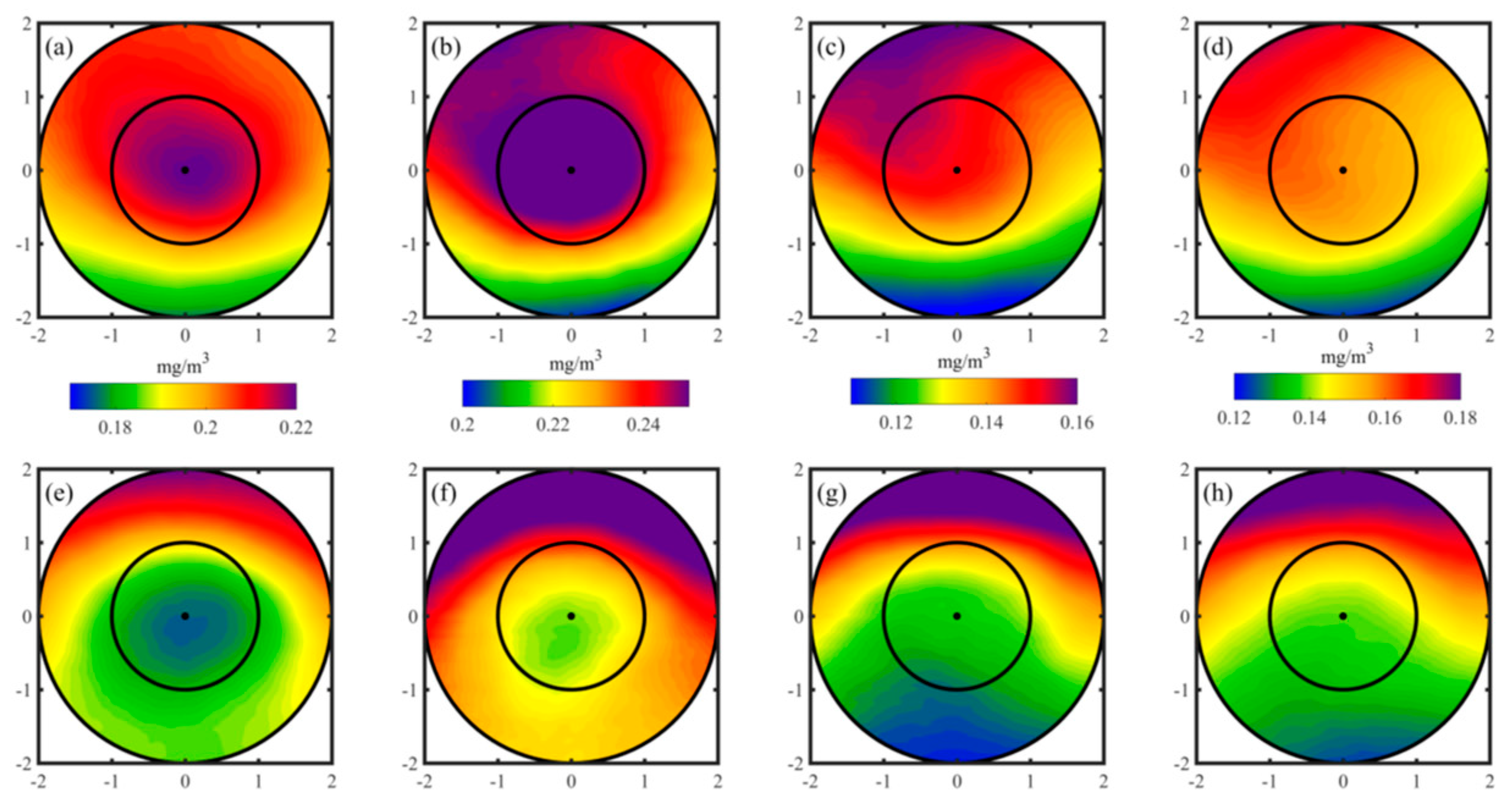
Figure 4.
The first three spatial empirical orthogonal function (EOF) mode of Chl-a within Cyclonic eddy in winter (first column),spring (second column), summer (third column) and autumn (fourth column).
Figure 4.
The first three spatial empirical orthogonal function (EOF) mode of Chl-a within Cyclonic eddy in winter (first column),spring (second column), summer (third column) and autumn (fourth column).
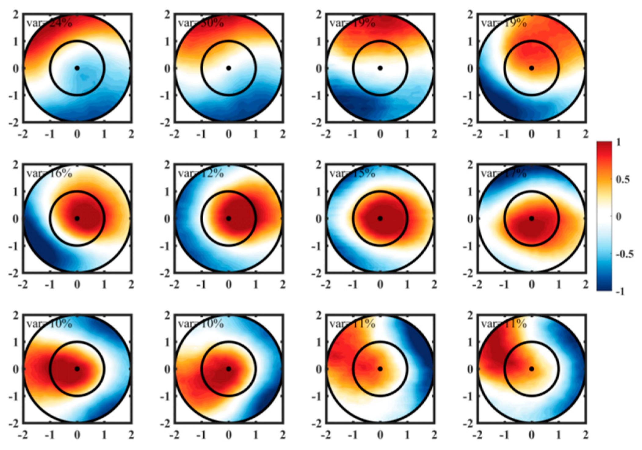
Figure 5.
The first three spatial empirical orthogonal function (EOF) mode of Chl-a within Anticyclonic eddy in winter (first column), spring (second column), summer (third column) and autumn (fourth column).
Figure 5.
The first three spatial empirical orthogonal function (EOF) mode of Chl-a within Anticyclonic eddy in winter (first column), spring (second column), summer (third column) and autumn (fourth column).
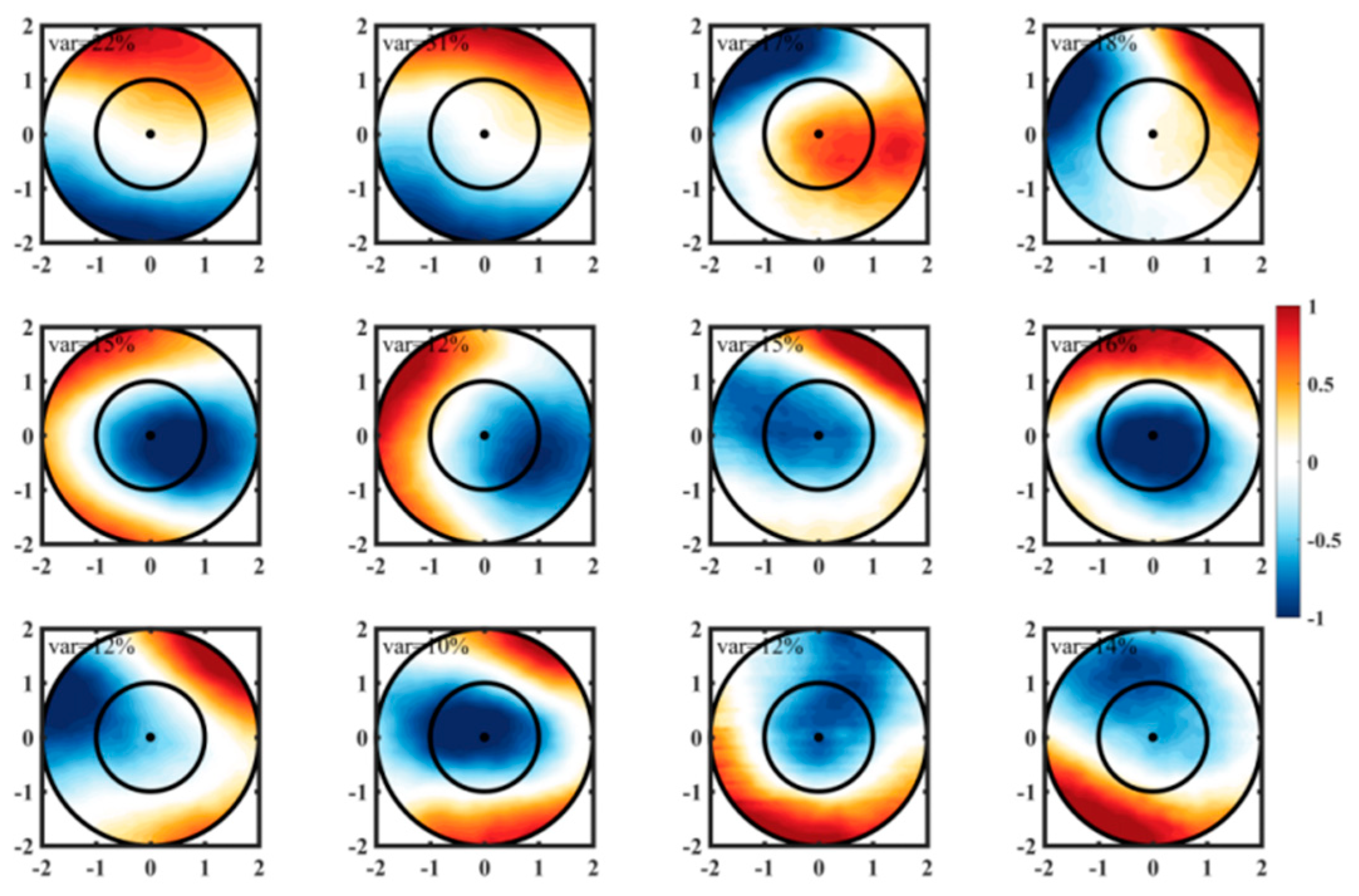
Figure 6.
Mean regional winter (a,b,c), spring (d,e,f), summer (g,h,i) and autumn (j,k,l) Chl-a anomalies within Cyclonic and Anticyclonic eddy in the KE during the period 1998 to 2016. Quantified at each 0.5 × 0.5 pixel.
Figure 6.
Mean regional winter (a,b,c), spring (d,e,f), summer (g,h,i) and autumn (j,k,l) Chl-a anomalies within Cyclonic and Anticyclonic eddy in the KE during the period 1998 to 2016. Quantified at each 0.5 × 0.5 pixel.
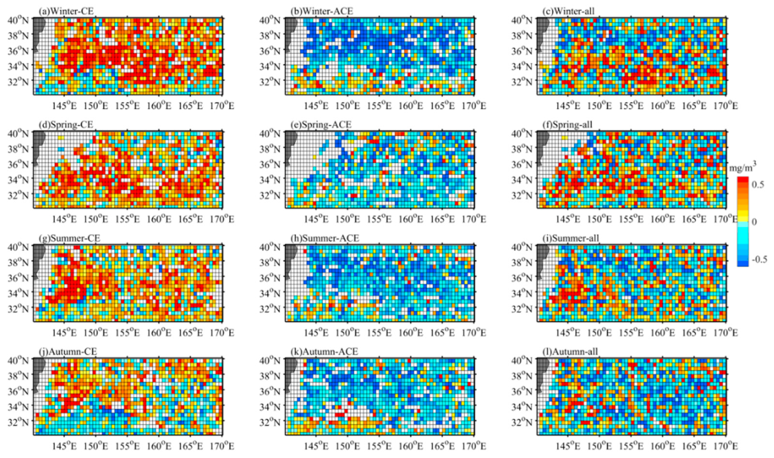
Figure 7.
Vertical profiles of temperature in eddies during winter(a), spring(b), summer(c) and autumn(d). Composite mean vertical profiles for cyclonic eddies (pink), anticyclonic eddies (blue), and edge (green). N indicates the number of profiles. The shading are standard errors. Dotted line represents mixed layer depth.
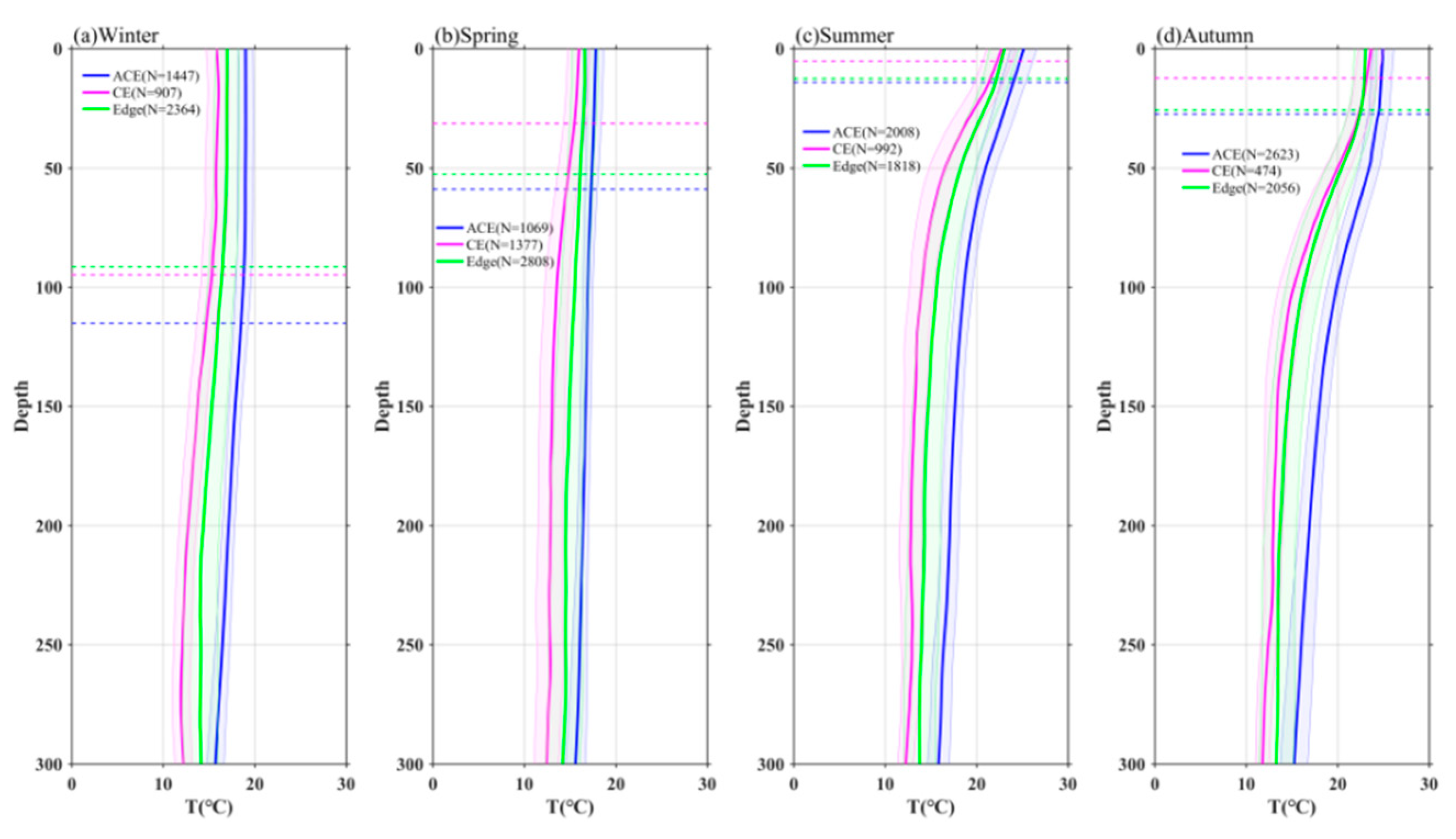
Figure 8.
Vertical profiles of Chl-a in eddies during winter(a), spring(b), summer(c) and autumn(d). The shading are standard errors.
Figure 8.
Vertical profiles of Chl-a in eddies during winter(a), spring(b), summer(c) and autumn(d). The shading are standard errors.
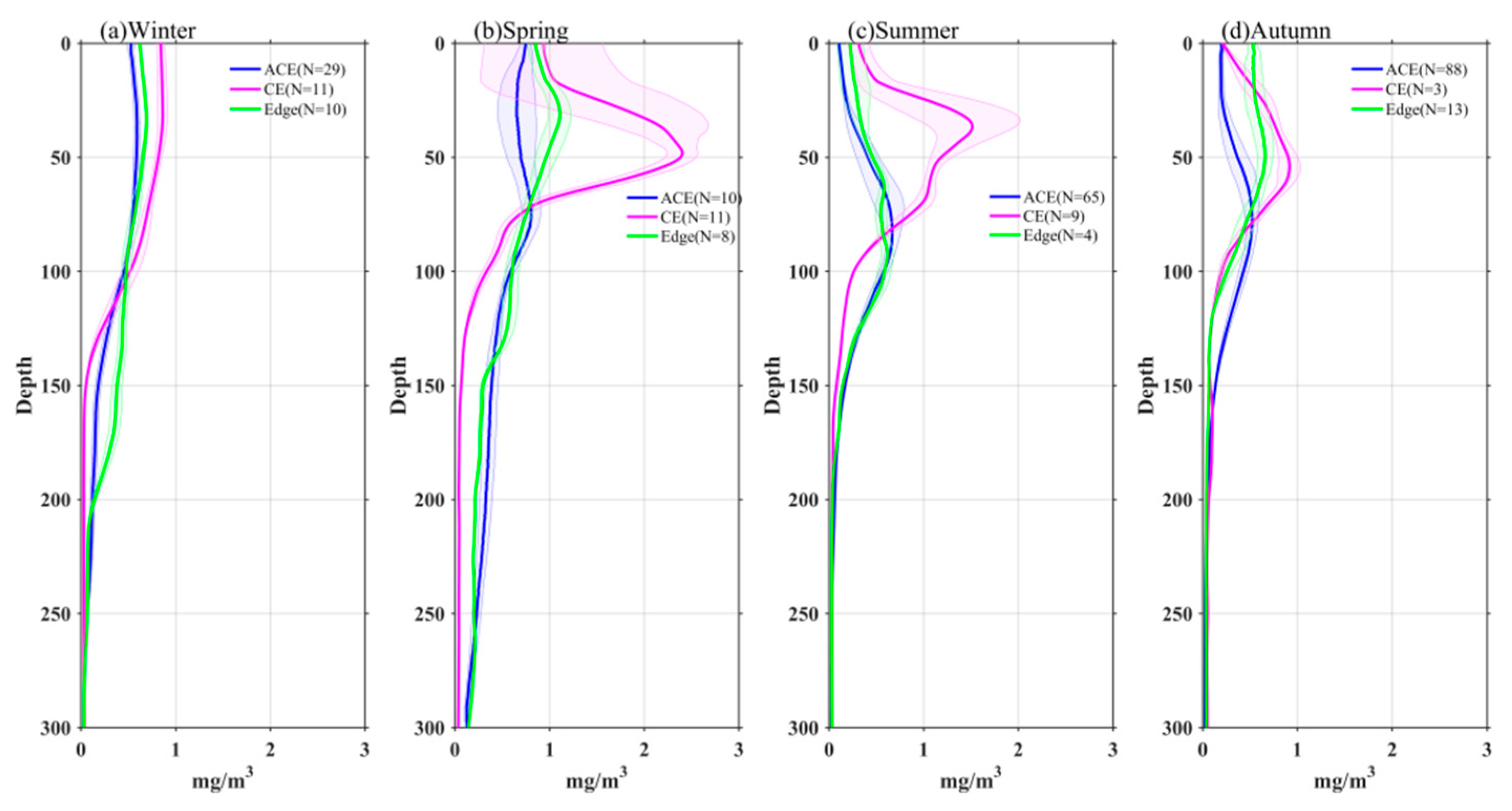
Figure 9.
Vertical profiles of nitrate in eddies during winter(a), spring(b), summer(c) and autumn(d). The shading are standard errors.
Figure 9.
Vertical profiles of nitrate in eddies during winter(a), spring(b), summer(c) and autumn(d). The shading are standard errors.
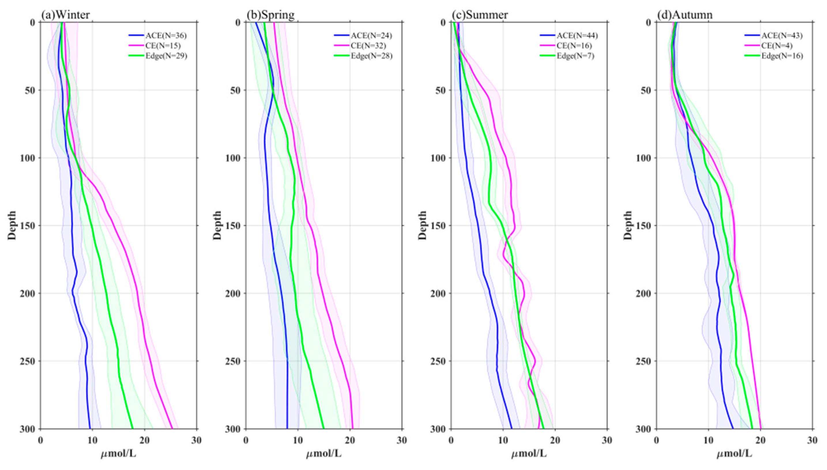
Figure 10.
Statistical relationship between the depth-integrated Chl-a (a), SCM(b), DSCM(c) and SLA. The blue, pink and green marks represent the observations in the CE, ACE and edge, respectively. The black solid lines are the linear regressions.
Figure 10.
Statistical relationship between the depth-integrated Chl-a (a), SCM(b), DSCM(c) and SLA. The blue, pink and green marks represent the observations in the CE, ACE and edge, respectively. The black solid lines are the linear regressions.
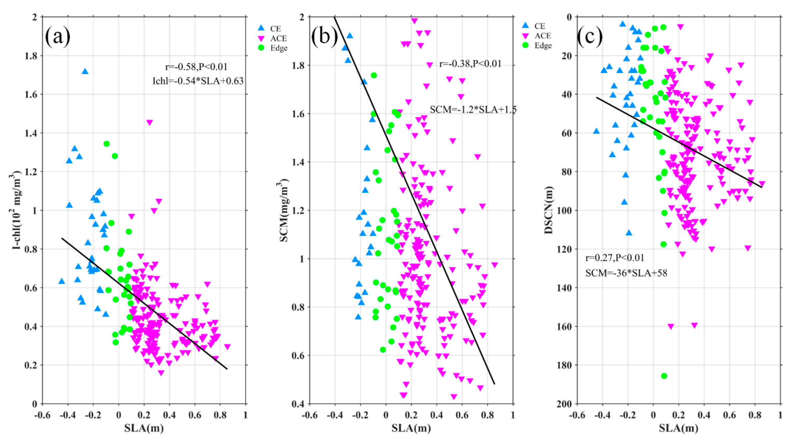
Figure 11.
Statistical relationship between the depth-integrated Chl-a(a), SCM(b), DSCM(c) and MLD. The blue, pink and green marks represent the observations in the CE, ACE, and edge, respectively. The black solid lines are the linear regressions.
Figure 11.
Statistical relationship between the depth-integrated Chl-a(a), SCM(b), DSCM(c) and MLD. The blue, pink and green marks represent the observations in the CE, ACE, and edge, respectively. The black solid lines are the linear regressions.
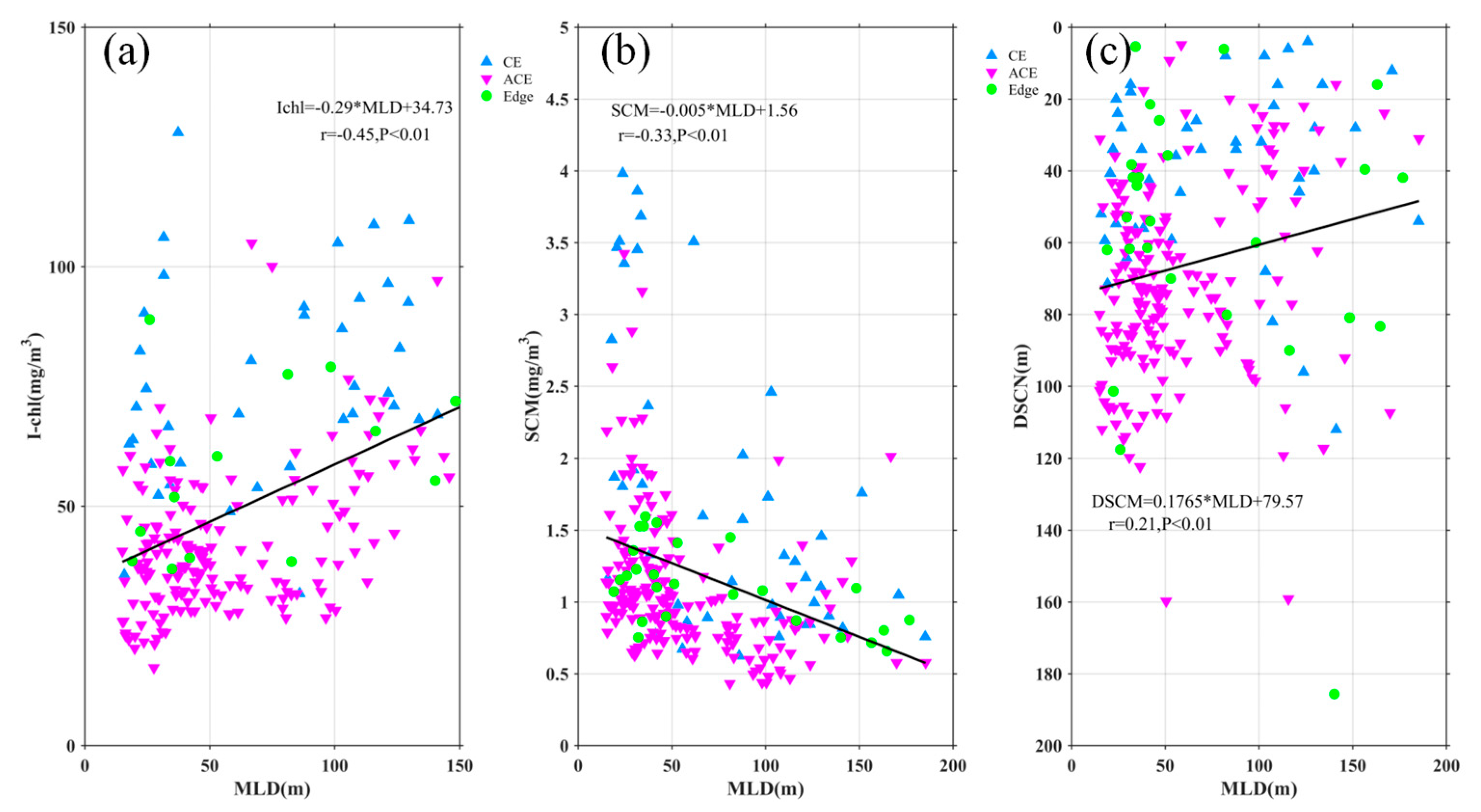
Figure 12.
Statistical relationship between the depth-integrated nitrate and SLA (a), MLD (b). The blue, pink and green marks represent the observations in the CE, ACE, and edge, respectively. The black solid lines are the linear regressions.
Figure 12.
Statistical relationship between the depth-integrated nitrate and SLA (a), MLD (b). The blue, pink and green marks represent the observations in the CE, ACE, and edge, respectively. The black solid lines are the linear regressions.
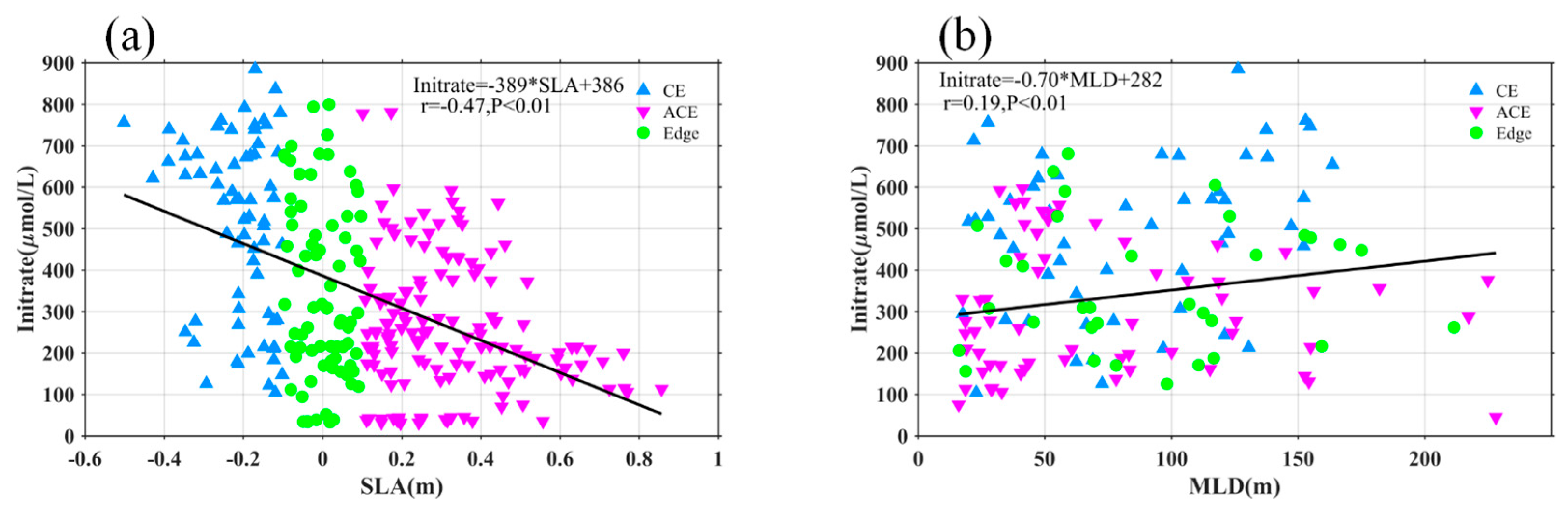
Figure 13.
Buoyancy frequency (shading) and MLD (blue and red lines)) from Argo floats within CEs (a) and ACEs (b) in KE. (c) buoyancy frequency difference between CEs and ACEs. The grey lines correspond to the nitrate mean seasonal contours.
Figure 13.
Buoyancy frequency (shading) and MLD (blue and red lines)) from Argo floats within CEs (a) and ACEs (b) in KE. (c) buoyancy frequency difference between CEs and ACEs. The grey lines correspond to the nitrate mean seasonal contours.
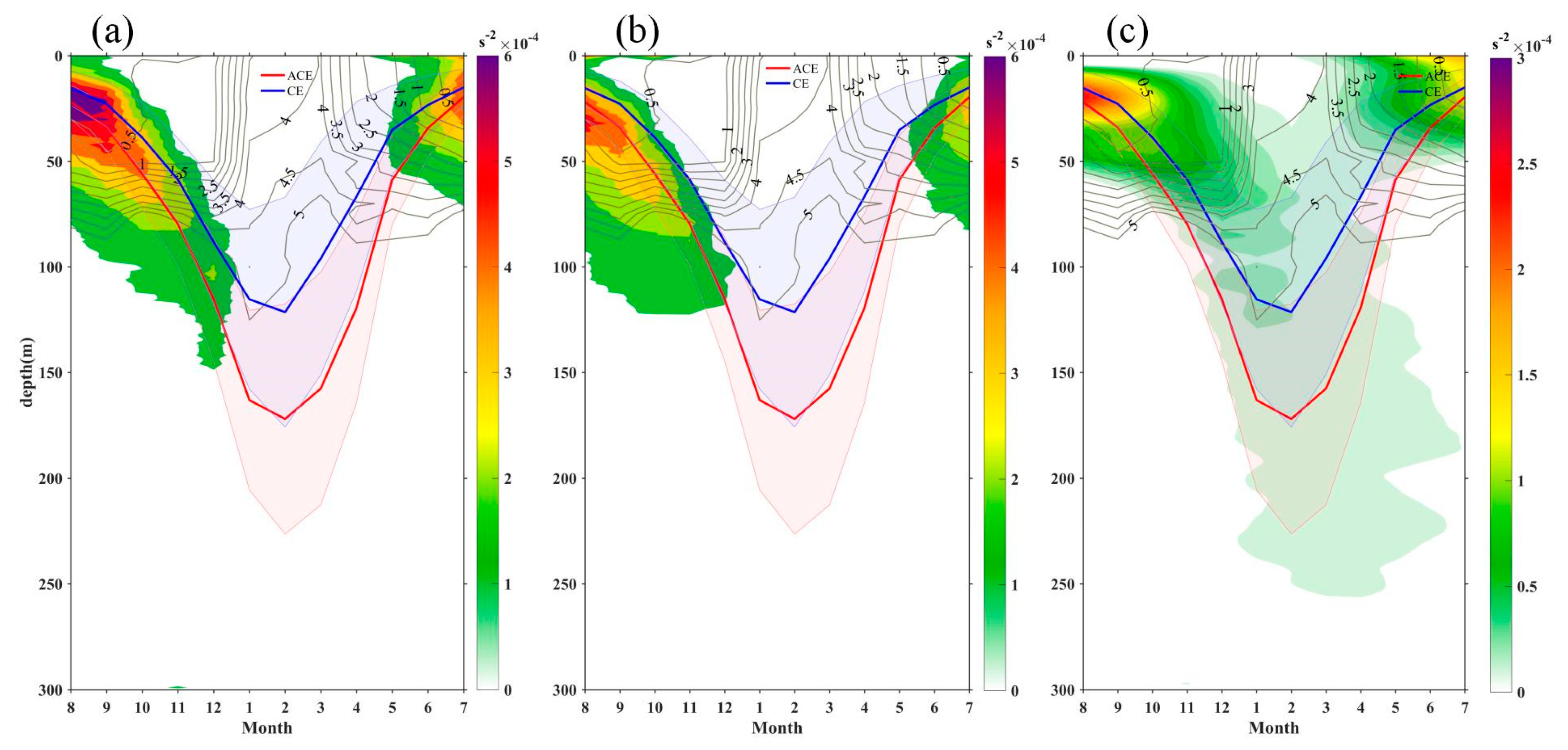
Figure 14.
The nitrogen budget analysis using the OFES hydrography-biology products provides estimates of nitrate changes (in mmol m−2 d−1) within the mixed layer during the winter period from 1999 to 2009. Four components are considered: (a) the total change in nitrate, (b) the mean advective-induced component (horizontal + vertical), (c) the eddy-induced component (horizontal + vertical), and (d) the mixing component.
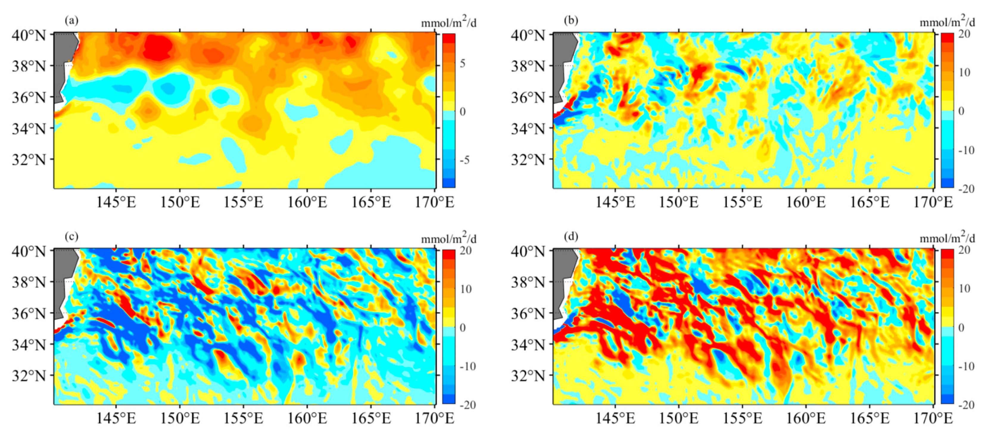
Figure 15.
The nitrogen budget analysis using the OFES hydrography-biology products provides estimates of nitrate changes (in mmol m−2 d−1) within the mixed layer during the summer period from 1999 to 2009. Four components are considered: (a) the total change in nitrate, (b) the mean advective-induced component (horizontal + vertical), (c) the eddy-induced component (horizontal + vertical), and (d) the mixing component.
Disclaimer/Publisher’s Note: The statements, opinions and data contained in all publications are solely those of the individual author(s) and contributor(s) and not of MDPI and/or the editor(s). MDPI and/or the editor(s) disclaim responsibility for any injury to people or property resulting from any ideas, methods, instructions or products referred to in the content. |
© 2023 by the authors. Licensee MDPI, Basel, Switzerland. This article is an open access article distributed under the terms and conditions of the Creative Commons Attribution (CC BY) license (http://creativecommons.org/licenses/by/4.0/).
Copyright: This open access article is published under a Creative Commons CC BY 4.0 license, which permit the free download, distribution, and reuse, provided that the author and preprint are cited in any reuse.


