
Submitted:
21 June 2024
Posted:
24 June 2024
You are already at the latest version
Abstract
The thermal conditions of transitional (ranging from warm to cold) coldwater streams impact the ranges and resource availabilities for biota inhabiting these lotic systems. With ongoing climate change and increasing land modifications, thermal boundaries may shift, altering thermal transition zones and their biotic communities. The objective of this study was to investigate the condition of trout across three forks of the Whitewater River catchment and to investigate factors influencing fish community composition and distribution. Each fork was characterized into three separate sections: headwater (coolwater), middle (warmwater), and lower (coldwater). Springs were identified throughout each fork, with greatest concentrations in the lower sections of each fork. Using single-pass electrofishing, we sampled 61 sites across the three forks in the Whitewater River system (North = 21 sites, Middle = 19, South = 21), and catch statistics were used to calculate diversity, trout abundance, and trout condition. In general, diversity increased, and trout were healthier but less abundant in middle and headwater sections, whereas diversity decreased slightly, trout condition decreased, and trout abundance increased in lower reaches, with changes differing somewhat among forks. Canonical correlation analysis had strong significant correlations showing simpson diversity and condition increase going upstream with high non trout abundance and catch rates while trout catch rates and reach width decrease. The Whitewater River is a catchment exhibiting transitional temperature-pattern characteristics with generally low fish community diversity and trout conditions that range from thin, normal, and robust. Dominated by a changing landscape (agriculture) and intensifying climate change, we may begin to see stream temperatures increase along with species diversity. Understanding how spring temperature influences species composition and distribution can bring potential stressors to light increasing our understanding of thermal conditions and to help mitigate the negative impacts from land use and climate change.
Keywords:
trout abundance
; climate change
; temperature pattern streams
; canonical correlation
; flow-chain model.
1. Introduction
Ecology is a discipline that seeks to understand why biological communities change over time [1]. As global climates change, it is important to understand and to predict how ecosystems and ecosystem services will respond to those changes [2]. As the severity of climate change increases, stream dynamics such as water temperature fluctuations [3], habitat changes and availability [4], and hydrological regime [5], become increasingly unstable, unpredictable, and highly variable [2]. Climate change, coupled with human activities that alter landscapes, can be drivers of change with the potential to negatively affect freshwater systems [6]. Often, landscapes are converted for agriculture, urban development, roadways or other municipal operations [7], and encroach on important floodplain features like riparian zones, and can have negative impacts on rivers [8]. The alteration of riparian zones (e.g., deforestation, grass and prairie removal) can alter lotic temperature regimes [9] and have deleterious effects on the natural structure and functioning of river ecosystems [10].
Climate change and land alterations are well known to affect streams and rivers. However, landscape type (such as karst geology) can further influence the structure and functioning of river ecosystems [11]. Karst landscapes have important hydrological influences on streams and rivers via groundwater exchange, providing biota with unique thermal refugia [12]. In karst terrain, groundwater processes have important moderating effects, reducing overall stream temperature and providing the cooler thermal regimes [12] needed by certain biota to complete their life histories [13]. Surface springs in karstic regions are extremely important for their influence on flow and temperature [14]. Springs can be variable in output volume and temperature depending on bedrock composition and complexity [15], which can influence the variability of stream temperatures [14]. Groundwater temperatures in karst landscapes can be governed by mean annual temperatures of the region in which those landscapes are located [14]. As climate change increases, mean annual atmospheric temperatures are expected to increase, this can have the potential of elevating aquifer (shallow aquifers can be more susceptible to warming) and groundwater temperatures and potentially increasing stream peak temperatures [16]. Consequently, the effects of increasing temperatures can act as a stressor and driver on biological communities, causing variability in populations [17].
Globally, 15.2% of the land surface is covered by karst [18]. Broken down, karst can be found in Europe (21.8%), North America (19.6%), Asia (18.6%), Africa (13.5%), Oceania (6.2%), and South America (4.3%) [18]. Karst dominates the landscape in portions of the upper midwestern USA, one of several such locations in North America. This region also is characterized as a sensitive bio-ecoregion [19], with streams exhibiting transitional, temperature-pattern stream networks supporting diverse communities. In this region, there is extensive dissolution and fracture of carbonate rock that accommodates large aquifers with extensive groundwater-surface water connectivity via springs and sinks. These springs stabilize flows and temperatures of receiving streams [15]. However, these conduit-type groundwater flow paths also produce rapid streamflow responses to rainfall, which can negatively alter hydrology and stream conditions [14].
Thermal refugia can be limiting to species distribution and composition [20,21], yet the variability of stream temperatures is known to be governed by climate change [22], groundwater [12], and changes to the riparian corridor [23] which can create unique temperature-driven stream patterns and communities. Transitional temperature-pattern streams are characterized by varying assemblages of warmwater, coolwater, and coldwater fish species occupying specific thermal habitats in karst regions [2,15]. As stream temperatures warm, certain species may become exposed to the dangers of shifting thermal regimes. Salmonids are of major concern, as they inhabit cold, groundwater-fed streams. Trout are generally sensitive fish with specific habitat and thermal requirements [24], have low thermal thresholds, and have high cultural, and recreational value [25].
Understanding the ecological effects of thermal inputs and changes in stream temperatures is paramount to predicting distributions of various species in sensitive regions. Karst regions are complex and thus present challenges toward this understanding, especially when these landscapes also are dominated by agriculture [26]. Stream temperatures can be influenced by atmospheric temperatures [27] and agricultural land modifications (forest removal, riparian removal) [6], but how biological communities respond to those changing temperatures is a knowledge gap requiring more research [12], especially in transitional temperature-pattern stream networks. In the present study, our objectives were to determine what effects thermal conditions may have on the distribution of different fish communities in a transitional temperature-pattern catchment in southeastern Minnesota, USA. Specifically, we examined fish communities and condition of trout within the transitional sections of streams along a longitudinal thermal gradient influenced by springs. We hypothesized that spring inputs would support the theory of the transitional temperature pattern and that fish communities would change along that thermal gradient. We hypothesize there will be important correlations in fish community distribution and trout condition.
2. Methodology
2.1. Study Area
Karst environments are dominated by soluble sandstone, limestone, dolomite, and shale [28]. Karst regions are among the most diverse hydrogeological environments, providing both valuable drinking water from aquifers and cold groundwater inputs to streams and rivers, as well as creating unique landscapes with sensitive biodiversity [18]. Forming 200 million years ago (mya) from deposited material under shallow seas, accumulations cemented together over time, forming layers of rock that are now the bluffs in southeastern Minnesota, southwestern Wisconsin, northeastern Iowa, and northwestern Illinois, collectively referred to as the Driftless Area (DA) ecoregion. During the most recent glacial advance ~10,000 years ago, the DA was left untouched by ice. Glacial meltwaters carved surrounding bluffs and plateaus, forming Mississippi River tributaries within an area > 25,900 km2, with > 27,000 km of fishable trout streams [29].
Located in southeastern Minnesota, USA, the Whitewater River is an agricultural catchment within the DA supporting a coldwater fishery. Home to native brook trout (Salvelinus fontinalis), introduced brown trout (Salmo trutta), stocked rainbow trout (Oncorhynchus mykiss), and slimy and mottled sculpin (family Cottidae; Uranidea cognata, Uranidea bairdii, respectively), sensitive species found throughout the catchment typically in coldwater sections. This catchment is comprised of three sub-catchments, the North, Middle, and South forks with >189 km of fishable, coldwater streams [6]. Together, the forks drain 829.6 km2 of agricultural land and mixed deciduous hardwood forest, across three counties (Olmsted, Winona, and Wabasha), joining together near Elba, Minnesota, and ultimately draining into the Mississippi River at Weaver, Minnesota, USA.
Each fork of the Whitewater River catchment, North, Middle, and South, are temperature-transitional sub-catchments. They are arranged from headwaters (HW), middle sections (MS), and lower sections (LS); coolwater, warmwater, and coldwater, respectively. A previous study [30] characterized each fork by section based on physical habitat, benthic macroinvertebrate index of biotic integrity, and fish index of biotic integrity. Our designations can be supported by stream management plans obtained from the Minnesota Department of Natural Resources Fisheries section in Lanesboro, Minnesota, USA. Each fork has specific designations for coldwater sections, in river miles, beginning at the confluence of each stream, going upstream with lower 24.2 (North Fork), 23.3 (Middle Fork), and 20.8 (South Fork) of each fork are designated as coldwater. Crow Spring drains into the Middle Fork downstream of the coldwater cutoff and is technically the coldwater section of the Middle.
2.2. Stream Surveys
During late spring to early autumn (May – October) in 2018 and 2019, we conducted fish surveys at 61 sites within the three forks of the Whitewater River catchment (North = 21, Middle = 19, South = 21; Figure 1). Surveys were conducted at sites along each of the three river forks and within main tributaries to each fork. Sites included locations both on private lands (with landowner consent) and public lands (e.g., state parks and wildlife management areas). We attempted to select study sites every 1.5 km along each fork and main tributaries. However, some areas were inaccessible due to terrain and lack of roadways within all forks; there were spatial gaps between sites, especially along the lower reaches of each fork.
Fish assessments were completed to estimate abundance (trout and non-trout), Simpsons Diversity Index (SDI), fishing effort (CPUE), and relative weight (Wr, trout only, a measure of fish condition) within 150-m reaches at each stream sites across all forks. A single-pass electrofishing method (downstream to upstream, Smith-Root LR-24 electrofisher, two or three netters) was used to survey the fish community. Fish captured were identified, counted, only trout were weighed (g) and measured (total length, mm), all fish were returned to the stream after capture, except for a few specimens retained for later identification. We examined length/weight data for trout only, to investigate trout condition and potential influences. We used condition as a descriptor for relative weight (Wr) to describe trout as “thin” (< 89%), “normal” (90 – 100 %), and “robust” (> 100%).
2.3. Data Analyses
Data were analyzed using Program R version 3.5.1 (R Core Team 2018), and Microsoft Excel. Basic descriptive statistics were used to describe stream variables and catch statistic data (i.e., means, and standard deviation). Inferential statistical methods following [31] (e.g., analysis of variance [ANOVA], Chi-square goodness of fit analysis, two-sample t-test) were used as appropriate to test for differences across various measurements among study reaches.
Spring data were collected from the Minnesota Spring Inventory website (https://arcgis.dnr.state.mn.us/portal/apps/webappviewer/index.html?id=560f4d3aaf2a41aa928a38237de291bc: Accessed 10 March 2024). Spring data were used to describe their potential influence on the temperature pattern of each fork. Number of springs, flow rates, and temperature were described for each of three sections across all forks for characterization of sections.
We used Simpson’s Diversity Index [32] to describe diversity of fish among forks. SDI is a measure of diversity which considers the number of species present and the relative abundance of each species. To calculate SDI using catch statistics, we used the following formula
where n is the number of individuals of a single species, N is the number of individuals in the total sample. The resulting values lie between 0 (low diversity) and 1 (high diversity).
SDI = 1- (∑n (n - 1) / N (N – 1))
To calculate trout abundance, we used number of fish caught divided by reach length, then multiplied by 1609 km. For CPUE estimates, we used fish/min to describe catch rates from electrofishing.
To assess whether certain factors varied longitudinally, a linear regression model-least squares approach (lm) was used with river.km as the predictor and diversity, CPUE, and condition, separately, as a response. Linear regression is used to estimate the linear relationship between a response (dependent) and predictor (independent) variables.
Canonical Correlations (CanCorr) [33] was used to explore multivariate relationships among stream variables and catch statistics. CanCorr finds separate linear combinations for the stream and catch multivariate data sets that have the maximum correlation with each other; these are denoted as the first canonical variate pair. Subsequent pairs of canonical variates (i.e., second, third, and so on) are independent of all previous canonical variates and show relationships among variables after accounting for factors driving all previous canonical variates. However, correlation strength decreases for subsequent canonical variates, so approximate F-tests [33] were used to test for non-zero correlations between canonical variate pairs. Heliographs [34] of the correlations between all significant canonical variates and the stream variables and catch statistics were used to portray multivariate relationships among stream characteristics.
3. Results
3.1. Spring Distribution and Influence
In total, 61 sites across the three forks (North, Middle, South) of the Whitewater River catchment were sampled for select environmental variables and fish. We identified 26, 30, and 19 springs in the three forks, with the greatest concentrations in the lower sections across each fork (Figure 2). Chi-square analyses revealed significant differences in spring distributions among stream sections within each fork (Table 1), whereas Chi-square contingency table analysis detected significant differences in the distributional patterns of springs among forks (X2 = 9.3, DF =2, P = 0.05). Cumulative flow inputs into the lower sections of each fork were: 459 l/s (North), 3,978 l/s (Middle), and 1,854 l/s (South); chi-square contingency determined there were significant differences in flow inputs by section among the three forks (X2 = 290, DF = 4, P = < 0.0001). The coldest temperature inputs from springs occurred in the LS of each fork, with inputs ranging from 5 – 9.6 °C (Figure 3). ANOVA revealed there were no significant differences in temperature inputs by section in each fork (F = 0.40, DF = 2, P = 0.67).
3.2. Diversity
In total, 9974 fish representing 21 species were sampled across the 61 sites surveyed within the catchment. For a full listing of fish species and counts, see [30]. Diversity was calculated for each section (HW, MS, and LS), and we used a linear model (diversity – response, river fork – predictor) to determine if there were any longitudinal patterns in diversity. The model detected differences, indicating that fish community diversity increases significantly in the upstream direction (LS to HW; Table 2). In general, diversity was lowest in LS, highest in MS, and intermediate in the HW within each fork (Table 3; Figure 4). However, ANOVA was only able to confirm differences for the Middle and South forks.
3.3. CPUE and Trout Abundance Estimates
A linear model (cpue – response, river.km – predictor) was used to detect any longitudinal patterns among sections within each fork. The model detected a significant relationship, with high catch rates in the LS, intermediate in the MS, and lowest in the HW in each fork (Table 4). All forks followed the same pattern of trout distribution, with more fish caught in the LS, to fewer in the MS, and the fewest trout caught in the HW sections. Distribution was uneven throughout sections; however, trout were present in all sections of each fork.
Trout abundance is an extrapolation of CPUE and was thus not modeled, as we expected the same outcome. Trout were most abundant in the Middle Fork with an estimated 338 trout/km in the LS, whereas abundance was less among sections in the North and South forks (Table 4). Catch rates in the MS of the Middle Fork were very high. Among sections of each fork, trout abundance varied, with significant differences detected in the North and South forks, but no differences in the Middle Fork. ANOVA determined there were significant differences in trout abundance within section of the North and South forks but not the Middle Fork (Table 4).
3.4. Trout Condition
A linear model (river.km – response, condition - predictor) was used on condition data to determine if a longitudinal pattern exists. We detected significant differences in the model showing that the North and South forks were different than the Middle Fork (Table 5). Within sections, trout condition differed significantly in the North and South forks but not in the Middle Fork (Table 6). The North and South forks followed the same pattern of robust trout in the HW’s, normal trout in the MS, and thin trout in the LS, while condition was normal throughout each section of the Midde Fork. ANOVA determined there were differences in trout condition within sections of the North and South forks but not the Middle Fork (Table 6).
3.5. Modeling
CanCorr modeling was used to further investigate the correlation structure between select non-catch and stream variables (x) to catch statistics (Y) to determine drivers of condition and trout distribution. The model produced a total of three canonical variate pairs, of which the first two showed significant correlation strength significantly different from zero (p < 0.05; Table 7). Heliographs revealed variables with strong correlations in describing potential drivers of population dynamics (Figure 5). The first canonical variate of the data sets had 76% significant correlation and showed that as river.km increases (upstream) in narrow reaches with high non-trout.min, diversity increases with fewer trout.min but in better condition. The second canonical variate had 51% significant correlation and showed that as reach width narrows (with river.km effect removed), catch rates (i.e., trout, non.trout) and condition increases, while diversity decreased.
4. Discussion
4.1. Major Findings
Karst landscapes provide features such as surface springs and aquifers that contribute greatly to transitional temperature patterns of streams and govern fish communities through thermal refugia. This study focused on investigating the effects thermal conditions may have on fish communities and distribution in a transitional temperature-pattern catchment in southeastern Minnesota, USA. First, springs were useful in characterizing the different river sections LS, MS, and HW associated with coldwater, warmwater, and coolwater transitional zones, respectively. Second, diversity showed a disjunct, non-linear pattern; communities were not distributed evenly as we hypothesized, but important details emerged with unexpected high SDI values in the coldwater LS portions of the North and South forks. Third, we detected an inverse relationship between trout abundance and condition that follows a linear pattern from LS to HW; high trout abundance means normal to thinner fish, moderate abundance = normal trout, and very low abundance = robust trout. Lastly, non-trout abundance was used in modeling to explore whether non-trout fish had an influence on trout condition; this supports the theory that trout are feeding on warmwater fish species with minimal intra-specific competition.
Findings from this study suggest the potential underlying factors governing temperature patterns, fish communities, and trout condition may be related to climate change and land use effects, among other factors. Climate change effects on river ecosystems is an area that is well understood, with many ecological changes attributed to warming temperatures [12,35]. Rising temperatures due to climate change, has a dampening effect in shallow aquifers [12] and may impact the temperature pattern of streams [36], as well as species composition and distribution [20], in karstic regions like those in southeastern Minnesota. Karstic regions are sensitive to biophysical changes [2] and the effects from climate change in the Whitewater River catchment may already be evident. We determined each fork exhibited a specific temperature pattern from cool to warm to cold (from the headwaters to downstream) related to spring inputs. However, we determined that the distribution and composition of fishes may be increasing in coldwater sections. Only the Middle Fork exhibited the pattern we expected with low (LS), high (MS), and moderate (HW) diversity. This may be explained as the LS of the Middle was heavily influenced by spring inputs (flow and temperature), likely from deep, well insulated aquifers [14]. Our findings are likely the result of rising temperatures, although, it is important to note, this study did not measure climate change-related components. The catchment is showing signs of increased diversity in sections where diversity should be low, both LS and HW. Only the Middle Fork showed the expected patterns of a transitional temperature-pattern stream, from cold to warm to cool.
Land use habits have been known to cause negative impacts to lotic systems from agriculture [6], roadways [37], and deforestation [38]. Agricultural streams in karst regions can be negatively impacted by hydrological events that deliver an excess amount of warmwater runoff [2], increased sediment loads, and nutrients [39], causing localized extirpation or displacement of biological communities [40]. Additional agricultural features can be sub-surface drain tile that can act as a rapid delivery system for shallow infiltrated water and may alter temperature regimes [35]. The Whitewater River catchment is located within a landscape altered for agriculture, with > 70% of the surrounding land converted [6]. Our findings led us to believe that temperature inputs may be allowing brown trout to travel further upstream into designated warmwater sections, dominated by agriculture, feeding on warmwater fish species. Trout were sparse, but in better condition in these sections than trout observed in the coldwater sections, where there are many and thinner trout. Streams may be warming due to land alterations but may be kept cool enough by sub-surface drain tiling for trout to thrive. The effects from climate change and land alterations on river ecosystems can be viewed through the lens of a conceptual model to put theories into perspective [41].
4.2. Conceptual Framework and Implications
Conceptual frameworks are increasingly used to understand complexity in environmental systems, such as the one in the present study. Flow chain models demonstrate interactions between various components of complex adaptive systems at multiple scales. Flow chain models have been used to demonstrate the efficiencies of environmental flow regimes on biophysical processes [41] and the ecological concept of disturbance in river systems [42]. Flow-chain models have four basic components representing the interplay of biophysical and social characteristics in river ecosystems (see Figure A below). Drivers are the main agents of change; functions are a series of controllers or processes that are governed by the agents of change; templates are those surfaces (both abiotic and biotic) upon which drivers and functions act; and finally, there are a series of responders, which can be sets of processes or actors that are parts of the social-ecological environment present across river ecosystems.
A flow chain model of the distribution of coldwater refugia (Figure A) shows their spatial array across the Whitewater River network to be the product of multiple biophysical interactions. The flow regime and water temperature are the main drivers that act upon the geomorphological structure of the riverine landscape. The output of this interaction, the altered physical template, directly influences the potential assemblage of coldwater refugia within the river network - the type, abundance, and position in the network [43]. Controllers, such as fish population density, competition, and social influences like fishing intensity, influence community structure of coldwater fishes within the network. Controllers interact via a series of interactions between the provision of coldwater refugia and coldwater fish community composition. Overall, this framework helps to understand the complex relationships between drivers, the physical template, and responses (ecological) and ecosystem services (social) within coupled riverine landscapes.
The ramifications from both climate change and land use habits are both seen and felt across the world. For example, as temperatures rise, oxygen concentrations, reproduction, and other various fish life history components decline, causing displacement or extirpation in rivers all around the world [44]. Thermal refugia created by groundwater or surface springs, at shallow depths, remain threatened by warming; many species are susceptible to temperature changes unless they are already adapted to variable water temperatures [12]. The continuing rise in temperatures may counter the effect of groundwater inputs (flow and temperature), so that species requiring colder temperatures may not be able to survive in this situation [45]. However, for deep aquifers, there is a buffering effect from warming climates. Aquifers are insulated beneath thick layers of rock, allowing for continuous coldwater flow inputs that help support sensitive species requiring these thermal regimes [14].
Thermal buffering from riparian corridors is known to moderate stream temperatures by shading stream channels [23]. There is a direct relationship from warming temperatures on the influence of stream temperatures when riparian corridors are modified due to land use [46], for example, when width of the buffer is narrow and other vegetation removed [47]. The effects from land use and its associated alterations are reported to negatively impact not only stream temperatures but extirpate local communities and cause long-term shifts in composition [48]. Proper management of the land and how it is used can enhance stream temperatures and community composition, but also recharge groundwater, ensuring its thermal integrity [14]. Recent studies have shown the positive effects of enhancing riparian features, for both stream temperatures and water quality [23,49,50]. Thermal regimes are controlled by exchanges with air temperature and groundwater [27]. Understanding the complexity of these relationships and how communities are influenced (i.e., distribution and composition) by such interactions is important to predicting how lotic systems are responding to change. Climate change and land use habits are known to be drivers of both thermal regimes [27] and the biological assemblages associated with temperature pattern-driven streams influenced by groundwater [36]. Under the current conditions, we may see changes in biological communities. Consider a flow chain model (Figure B) to attempt to predict how river ecosystems may respond. In a scenario with minimal stressors (i.e., no climate change, natural landscape), a natural setting exists. Under a natural setting, a typical set of conditions for a particular stream in a karst region in southeastern Minnesota are characterized. These will be influenced by changing conditions (disturbances) via land use. The result may be a new set of conditions as a response to land use. Now, couple land use with climate, creating yet again a different set of conditions. Each change has implications for the current physical structure (habitat) and its proper functioning (communities).
5. Conclusions
Thermal regimes in agricultural streams in karst landscapes are influenced by groundwater processes and atmospheric temperatures [14]. Underlying drivers of many biological processes in lotic systems and consequently biological assemblages, are related to variable stream temperature inputs [36]. Our findings indicate that groundwater likely was most influential in driving temperature patterns and the distribution and condition of trout. We believe there are short comings and knowledge gaps in our study as expected, but the findings appear sound. The complexity of the influence of warming climate and land use on biological assemblages could be studied further. Many studies with related findings suggest that the impacts from drivers can be mitigated with proper land management practices [2,12,14,21,36], and by doing so, changes may be minimal or non-existent. Proper land management is especially important in karst regions with coldwater streams and salmonids as inhabitants, as recreational activities help economically to sustain local communities [6].
Acknowledgments
We thank the private landowners who granted us permission to access the river for this study. A. Varela, C. Weaver, T. Biederman, O. Graziano, and others that assisted with fish surveys. Dedicated to Mark White (Forestville State Park, MN), for our conversations on groundwater movement in karst regions. .
Ethics approval - Compliance with ethical standards
Fish surveys were made under special permits (Numbers 12769, 23668, 28374) from the Minnesota Department of Natural Resources, Division of Fish and Wildlife, Section of Fisheries, and were conducted with the approval of the Winona State University Institutional Animal Care and Use Committee (1317064-1, 1310072-2). This research complied with all ethical standards.
Author Contributions
WV and NM developed the concept for the paper. WV, NM, CW, and JCB participated in field work consisting of stream surveys. WV and DS performed the analyses, SB conducted additional analyses, and WV led the writing of the paper. MT assisted with conceptual model development and understanding and made contributions to the discussion. (All authors will edit the manuscript and eventually accept the submitted version.).
Funding
This project was funded by the Minnesota’s Environment and Natural Resources Trust Fund, as recommended by the Legislative-Citizen Commission on Minnesota Resources (M.L. 2017, Chp. 96, Sec. 2, Subd. 04d / Water Quality Monitoring in Southeastern Minnesota Trout Streams).
Conflicts of Interest
The authors declare no competing interests.
References
- Connell, J.H.; Sousa, W.P. On the evidence needed to judge ecological stability or persistence. Am. Nat. 1983, 121, 789–824. [Google Scholar] [CrossRef]
- Hitt, N.P.; Rogers, K.M.; Kessler, K.G.; Briggs, M.A.; Fair, J.H. Stabilising effects of karstic groundwater on stream fish communities. Ecol Freshw Fish, 2022, 32, 538–551. [Google Scholar] [CrossRef]
- Kaushal, S.S.; Likens, G.E.; Jaworski, N.A.; Pace, M.L.; Sides, A.M.; Seekell, D.; Belt, K.T.; Secor, D.H.; Wingate, R.L. Rising stream and river temperatures in the United States. Front. Ecol. Environ. 2010, 8, 461–466. [Google Scholar] [CrossRef]
- Van Meerbeek, K.; Jucker, T.; Svenning, J. Unifying the concepts of stability and resilience in ecology. J. Ecol. 2021, 109, 3114–3132. [Google Scholar] [CrossRef]
- Hitt, N.P.; Rogers, K.M.; Kelly, Z.A.; Henesy, J.; Mullican, J.E. Fish life history traits indicate increasing flow stochasity in an unregulated river. Ecosphere, 2020, 11, e03026. [Google Scholar] [CrossRef]
- arela, W.L.; Mundahl, N.D.; Staples, D.F.; Greene, R.H.; Bergen, S.; Cochran-Biederman, J.; Weaver, C.R. Influence of Riparian Conditions on Physical Instream Habitats in Trout Streams in Southeastern Minnesota, USA. Water, 2024, 16, 864. [Google Scholar] [CrossRef]
- Brierley, G.J. “The socio-ecological river, Socio-economic, cultural and environmental relations to river systems”. Finding the Voice of the River: Beyond Restoration and Management. Springer International Publishing AG. 2020, 29-60.
- Graziano, M.P.; Deguire, A.K.; Surasinghe, T.D. Riparian Buffers as a Critical Landscape Feature: Insights for Riverscape Conservation and Policy Renovations. Diversity. 2022, 14, 172. [Google Scholar] [CrossRef]
- Opperman, J.J.; Merenlender, A.M. The effectiveness of Riparian Restoration for Improving Fish Habitat in Four Hardwood-Dominated California Streams. North Am. J Fish. Manage. 2004, 24, 822–834. [Google Scholar] [CrossRef]
- Thorp, J.H.; Thoms, M.C.; Delong, M.D. The Riverine Ecosystem Synthesis: Toward Conceptual Cohesiveness in River Science. Academic Press: London, UK, 2008.
- Magoulick, D.D.; Dekar, M.P.; Hodges, S.W.; Scott, M.K.; Rabalais, M.R.; Bare, C.M. Hydrologic variation influences stream fish assemblage dynamics through flow regime and drought. Sci. Rep. 2021, 11, 10704. [Google Scholar] [CrossRef]
- Kaandorp, V.P.; Doornenbal, P.J.; Broers, H.P.; de Louw, P.G.B. Temperature buffering by groundwater in ecologically valuable lowland streams under current and future climate conditions. J. Hydrol.X, 2019, 3, 100031. [Google Scholar] [CrossRef]
- Mims, M.C.; Olden, J.D. Life history theory predicts fish assemblage response to hydrologic regimes. Ecology 2012, 93, 35–45. [Google Scholar] [CrossRef]
- Krider, L.A.; Magner, J.A.; Perry, J.; Vondracek, B.; Ferrington Jr., L. C. Air-water temperature relationships in the trout streams of southeastern Minnesota’s carbonate-sandstone landscape. J. Am. Water Resour. Assoc. 2013, 49, 896–907. [Google Scholar] [CrossRef]
- Luhmann, A.J.; Covington, M.D.; Peters, A.J.; Alexander, S.C.; Anger, C.T.; Green, J.A.; Runkel, A.C.; Alexander Jr., E. C. Classification of Thermal Patterns at Karst Springs and Cave Streams. Ground Water, 2011, 49, 324–335. [Google Scholar] [CrossRef]
- Watts, G.; Battarbee, R.W.; Bloomfield, J.P.; Crossman, J.; Daccache, A.; Durance, L.; Elliot, J.A.; Garner, G.; Hannaford, J.; Hannah, D.M.; Hess, T.; Jackson, C.R.; Kay, A.L.; Kernan, M.; Knox, J.; Mackay, J.; Monteith, D.T.; Ormerod, S.J.; Rance, J.; Stuart, M.E.; Wade, A.J.; Wade, S.D.; Weatherhead, K.; Whitehead, P.G.; Wilby, R.L. Climate change and water in the UK – past changes and future prospects. Prog. Phys. Geogr. 2015, 39, 6–28. [Google Scholar] [CrossRef]
- Woodward, G.; Perkins, D.M.; Brown, L.E. Climate change and freshwater ecosystems: impacts across multiple levels of organization. Phil. Trans. R. Soc. 2010, 365, 2093–2106. [Google Scholar] [CrossRef]
- Goldscheider, N.; Chen, Z.; Auler, A.S.; Bakalowicz, M.; Broda, S.; Drew, D.; Hartmann, J.; Jiang, G.; Moosdorf, N.; Stevanovic, Z.; Veni, G. Global distribution of carbonate rocks and karst water resources. Hydrogeol. J. 2020, 28, 1661–1677. [Google Scholar] [CrossRef]
- Omernik, J.M. Ecoregions of the conterminous United States. Ann. Assoc. Am. Geogr. 1987, 77, 118–125. [Google Scholar] [CrossRef]
- Isaak, D.J.; Luce, C.; Horan, D.L.; Chandler, G.L.; Wollrab, S.P.; Nagel, D.E. Global warming of salmon and trout Rivers in the Northwestern U.S.: road to ruin or path through purgatory? Trans. Am. Fish. Soc. 2018, 147, 566–587. [Google Scholar] [CrossRef]
- Kaandorp, V.P.; Molina-Navarro, E.; Andersen, H.E.; Bloomfield, J.P.; Kuijper, M.J.M.; de Louw, P.G.B. ; A conceptual model for the analysis of multi-stressors in linked groundwater-surface water systems. Sci. Total Environ. 2018, 627, 880–895. [Google Scholar] [CrossRef]
- Hammond, J.C.; Simeone, C.; Hecht, J.S.; Hodgkins, G.A.; Lombard, M.; McCabe, G.; Wolock, D.; Wieczorek, M.; Olson, C.; Caldwell, T.; Dudley, R.; Price, A.N. Going beyond low flows: Streamflow drought deficit and duration illuminate distinct spatio-temporal drought patterns and trends in the U.S. during the last century. Water Resour. Res. 2022, 58, e2022WRO31930. [Google Scholar] [CrossRef]
- Mundahl, N.D.; Varela, W.L.; Weaver, C.; Mundahl, E.D.; Cochran-Biederman, J.L. Stream habitats and aquatic communities in an agricultural watershed: changes related to a mandatory riparian buffer law. Environ. Manage. 2023, 5, 945–958. [Google Scholar] [CrossRef] [PubMed]
- Dieterman, J.D.; Mitro, M.D. Stream Habitat Needs for Brook Trout and Brown Trout in the Driftless Area. A look back at driftless area science to plan for resiliency in an uncertain future. Special Publication of the 11th Annual Driftless Symposium, La Crosse, Wisconsin. 2019.
- Isaak, D.J.; Wollrab, S.; Horan, D.; Chandler, G. Climate change effects on stream and river temperatures across the northwest U.S. from 1980-2009 and implications for salmonid fishes. Clim. Change, 2012, 113, 499–524. [Google Scholar] [CrossRef]
- Bendorf, J.; Hubbard, J.; Kucharik, C.J.; VanLoocke, A. Rapid changes in agricultural land use and hydrology in the Driftless Region. Agrosystems Geosci. Environ. 2021, 4, e20214. [Google Scholar] [CrossRef]
- Webb, B.W.; Hannah, D.M.; Moore, R.D.; Brown, L.E.; Nobilis, F. Recent advances in stream and river temperature research. Hydrol. Process. 2008, 22, 902–918. [Google Scholar] [CrossRef]
- Mundahl, N.; Borsari, B.; Meyer, C.; Wheeler, P.; Siderius, N.; Harmes, S. Sustainable Management of Water Quality in Southeastern Minnesota, USA: History, Citizen Attitudes, and Future Implications. Sustainable Water Use and Management: Examples of New Approaches and Perspectives. Springer International Publishing, Cham. 2015.
- Iannicelli, M. Evolution of the Driftless Area and Contiguous Regions of Midwestern USA Through Pleistocene Periglacial Processes. The Open Geol. J. 2010, 4, 35–54. [Google Scholar] [CrossRef]
- Varela, W.L.; Mundahl, N.D.; Bergen, S.; Staples, D.F.; Cochran-Biederman, J.; Weaver, C.R. Physical and Biological Stream Health in an Agricultural Watershed after 30+ Years of Targeted Conservation Practices. Water 2023, 15, 3475. [Google Scholar] [CrossRef]
- Zar, J.H. Biostatistical Analysis. Prentice Hall Inc. Upper Saddle River, New Jersey. 1999.
- Simpson, E.H. Measurement of species diversity. Nature, 1949, 163, 688. [Google Scholar] [CrossRef]
- Rencher, A.C.; Christensen, W.F. Methods of Multivariate Analysis. Wiley Series in Probability Statistics 3rd edition. John Wiley and Sons Inc. 2012. [Google Scholar]
- Degani, A.; Shafto, M.; Olson, L. Canonical correlation analysis: Use of composite heliographs for representing multiple patterns. International Conference on Theory and Application of Diagrams. Berlin, Heidelberg: Springer Berlin Heidelberg. 2006, 93-97.
- Smith, E.A.; Gillete, T.; Blann, K.; Coburn, B.H.; Rhees, S. Drain tiles and groundwater resources: Understanding the relations. Minnesota Ground Water Association, 2018.
- Snyder, C.D.; Hitt, N.P.; Young, J.A. Accounting for groundwater in stream fish thermal habitat responses to climate change. Ecol. Appl. 2015, 25, 1397–1419. [Google Scholar] [CrossRef]
- Trimble, S.W., Jr.; Sartz, R.S. How far from a stream should a logging road be located? J. For. 1957, 55, 339–341. [Google Scholar]
- Meleason, M.A.; Gregory, S.V.; Bolte, J.P. Implications of Riparian Management Strategies on Wood in Streams of the Pacific Northwest. Ecol. Appl. 2003, 13, 1212–1221. [Google Scholar] [CrossRef]
- Dotterweich, M. The history of human-induced soil erosion: Geomorphic legacies, early descriptions and research, and the development of soil conservation-A global synopsis. Geomorphology 2013, 201, 1–34. [Google Scholar] [CrossRef]
- Roghair, C.N.; Dolloff, C.A.; Underwood, M.K. Response of a brook trout population and instream habitat to a catastrophic flood and debris flow. Trans. Am. Fish. Soc. 2002, 131, 718–730. [Google Scholar] [CrossRef]
- Yarnell, S.M.; Thoms, M.C. Enhancing the functionality of environmental flows through an understanding of biophysical processes in the riverine landscape. Front. Environ. Sci. 2022, 10, 787216. [Google Scholar] [CrossRef]
- Grimm, N.B.; Pickett, S.T.A.; Hale, R.L.; Cadenasso, M.L. Does the ecological concept of disturbance have utility in urban social-ecological-technological systems? Ecosyst. Health Sustain. 2017, 3, e01255. [Google Scholar] [CrossRef]
- Thoms, M.C.; Meitzen, K.M.; Julian, J.P.; Butler, D.R. Bio-geomorphology and resilience thinking: Common ground and challenges. Geomorphology, 2018, 305, 1–7. [Google Scholar] [CrossRef]
- Chopel, Y. Global Warming and Climate Change (GWCC) Realities. In The Nature, Causes, Effects and Mitigation of Climate Change on the Environment. 2022, 3. [Google Scholar]
- Kurylyk, B.L.; MacQuarrie, K.T.B.; Voss, C.I. Climate change impacts on the temperature and magnitude of groundwater discharge from shallow, unconfined aquifers. Water Resour. Res. 2014, 50, 3253–3274. [Google Scholar] [CrossRef]
- O’Driscoll, M.A.; DeWalle, D.R. Stream-Air Temperatures Relations to Classify Stream-Ground Water Interactions in a Karst Setting, Central Pennsylvania, USA. J. Hydrol. 2006, 329, 140–153. [Google Scholar] [CrossRef]
- Cristea, N.; Janisch, J. “Modeling effects of the riparian buffer width on effective shade and stream temperature”. Washington State Department of Ecology, 2007.
- Comte, L.; Olden, J.D.; Tedesco, P.A.; Ruhi, A.; Giam, X. Climate and land-use changes interact to drive long-term reorganization of riverine fish communities globally. Proc. Natl. Acad. Sci. USA 2021, 118, e2011639118. [Google Scholar] [CrossRef]
- Welcomme, R.L. Fisheries Ecology of Floodplain Rivers; Longman: London, UK, 1979. [Google Scholar]
- Death, R.G.; Collier, K.J. Measuring stream macroinvertebrate responses to gradients of vegetation cover: When is enough enough? Freshw. Biol. 2010, 55, 1447–1464. [Google Scholar] [CrossRef]
Figure 1.
Whitewater River catchment located in southeastern Minnesota, USA. Displayed are the North (n = 21), Middle (n = 19), and South Forks (n = 21) with main tributaries. The four-point stars are study sites along each fork. This catchment is dominated by agricultural activities with >70% of the once forested land converted.

Figure 2.
The distribution of springs in proportion form. Springs were unevenly distributed throughout each fork. The greatest concentrations were found in the LS’s of each fork near the confluence into the mainstem. Data retrieved from the Minnesota Spring Inventory website (https://arcgis.dnr.state.mn.us/portal/apps/webappviewer/index.html?id=560f4d3aaf2a41aa928a38237de291bc: Accessed March 2024) for the Whitewater River catchment located in southeastern Minnesota, USA.

Figure 3.
The occurrence of temperature inputs from springs into each fork. Most inputs were below 10 °C or 50 °F. Temperatures were arranged in bins of five-degree increments and sites were tallied based on temperature. Data retrieved from the Minnesota Spring Inventory website (https://arcgis.dnr.state.mn.us/portal/apps/webappviewer/index.html?id=560f4d3aaf2a41aa928a38237de291bc: Accessed 10 March 2024) for the Whitewater River catchment located in southeastern Minnesota, USA.
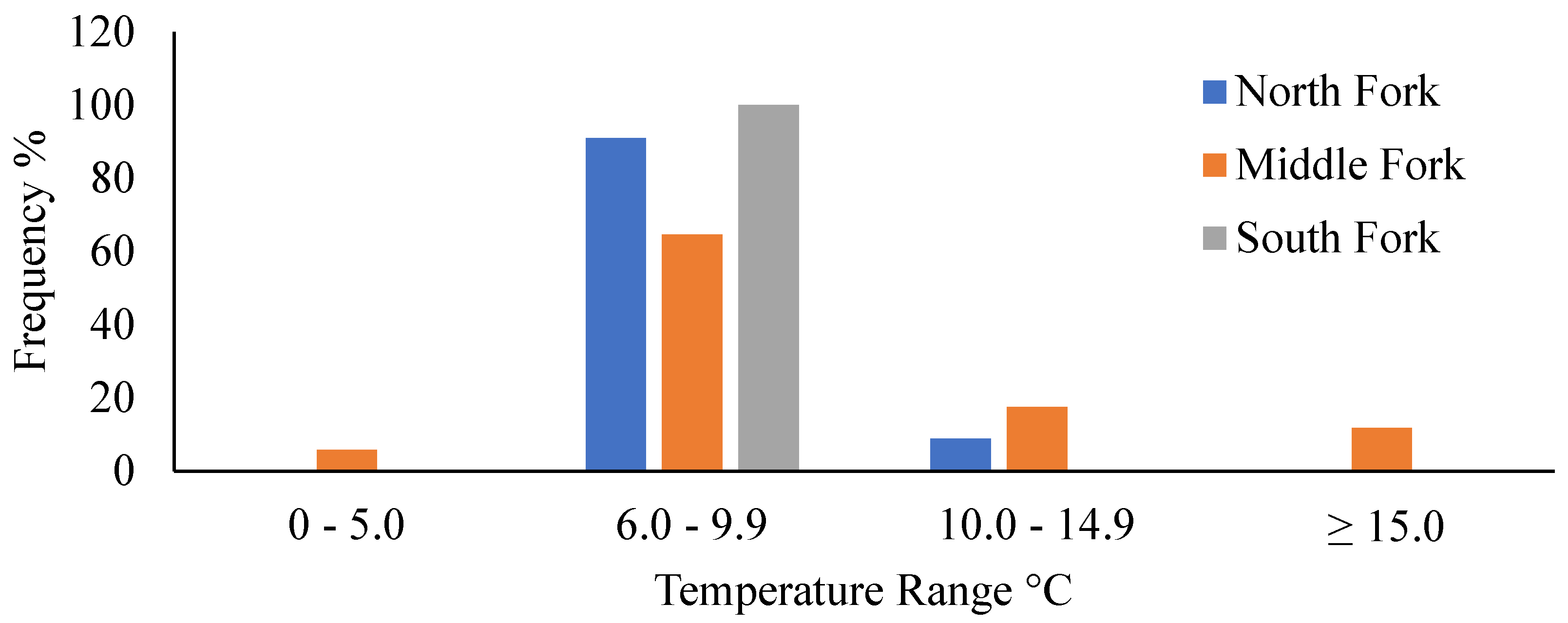
Figure 4.
Mean Simpson Diversity Index values are displayed with ± one standard deviation error bars. Data are arranged by section for each fork from the HW to LS’s sections. Data collected during late spring and early fall in 2018 and 2019 in the Whitewater River catchment in southeastern Minnesota, USA.
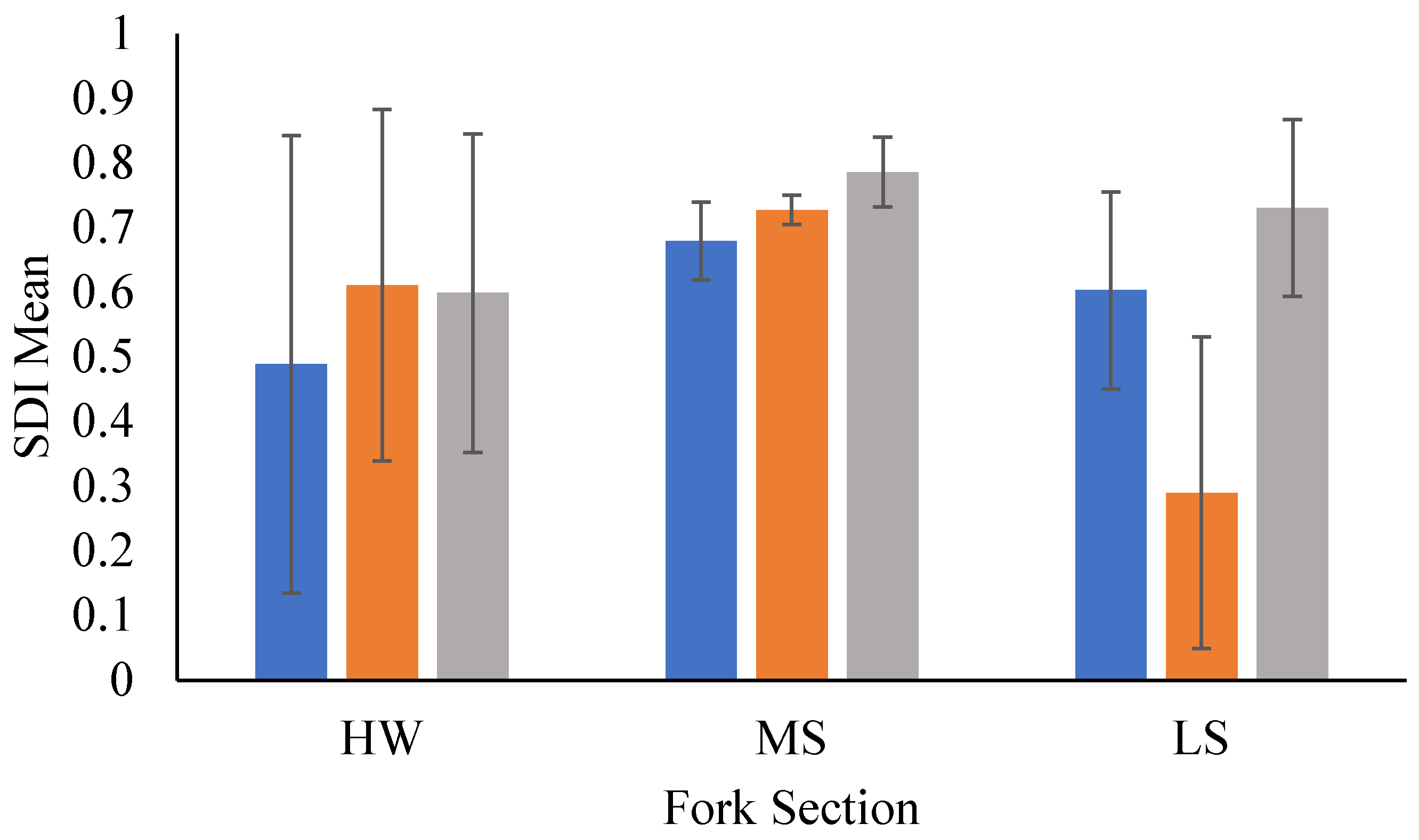
Figure 5.
Heliographs of the first two canonical variates from Canonical Correlation modeling displaying the correlation between canonical variates and associated stream variables (X) and catch statistics (Y). Length of bars are proportional to the absolute strength of the correlation; solid black vars are positive correlations, while clear bars show negative correlations plotted on polar coordinates. Data collected during late spring and early fall in 2018 and 2019 in the Whitewater River catchment in southeastern Minnesota, USA. Figure A. Conceptual social-ecological model. This describes the agents that shape the physical template of rivers, the altered template, those that control composition, and how communities respond to those agents/drivers of change. Developed for coldwater communities in southeastern Minnesota, USA. Figure B. Flow chain model depicting how rivers may respond to changes. Under a natural setting with natural conditions, some disturbance alters the natural setting, land use; from that interaction, a new set of conditions emerges. Then climate change coupled with land use may produce another set of conditions in river ecosystems. This model can be used to predict potential responses to change or drivers of change in river ecosystems. Flow chain model was developed for trout streams in southeastern Minnesota, USA.
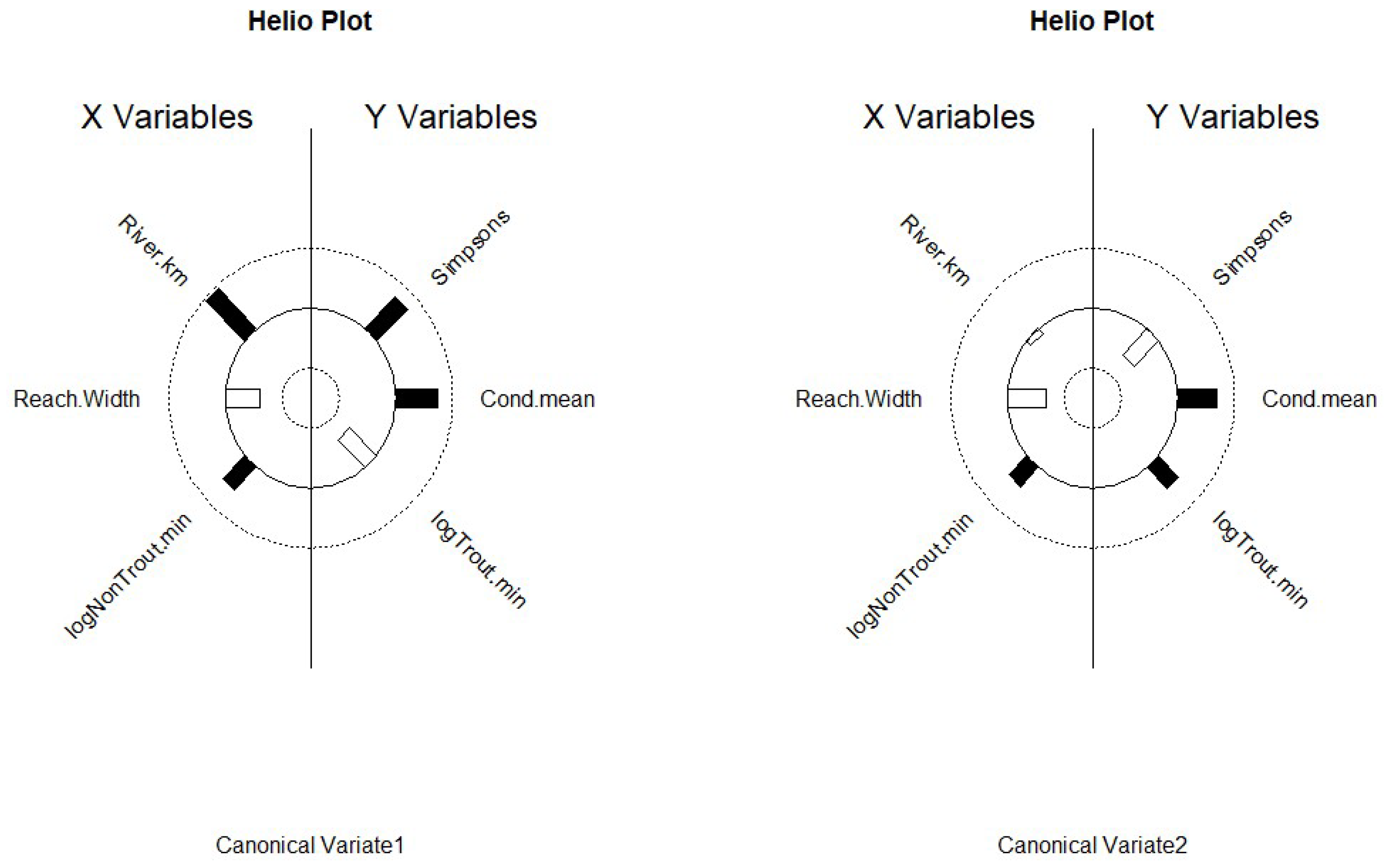
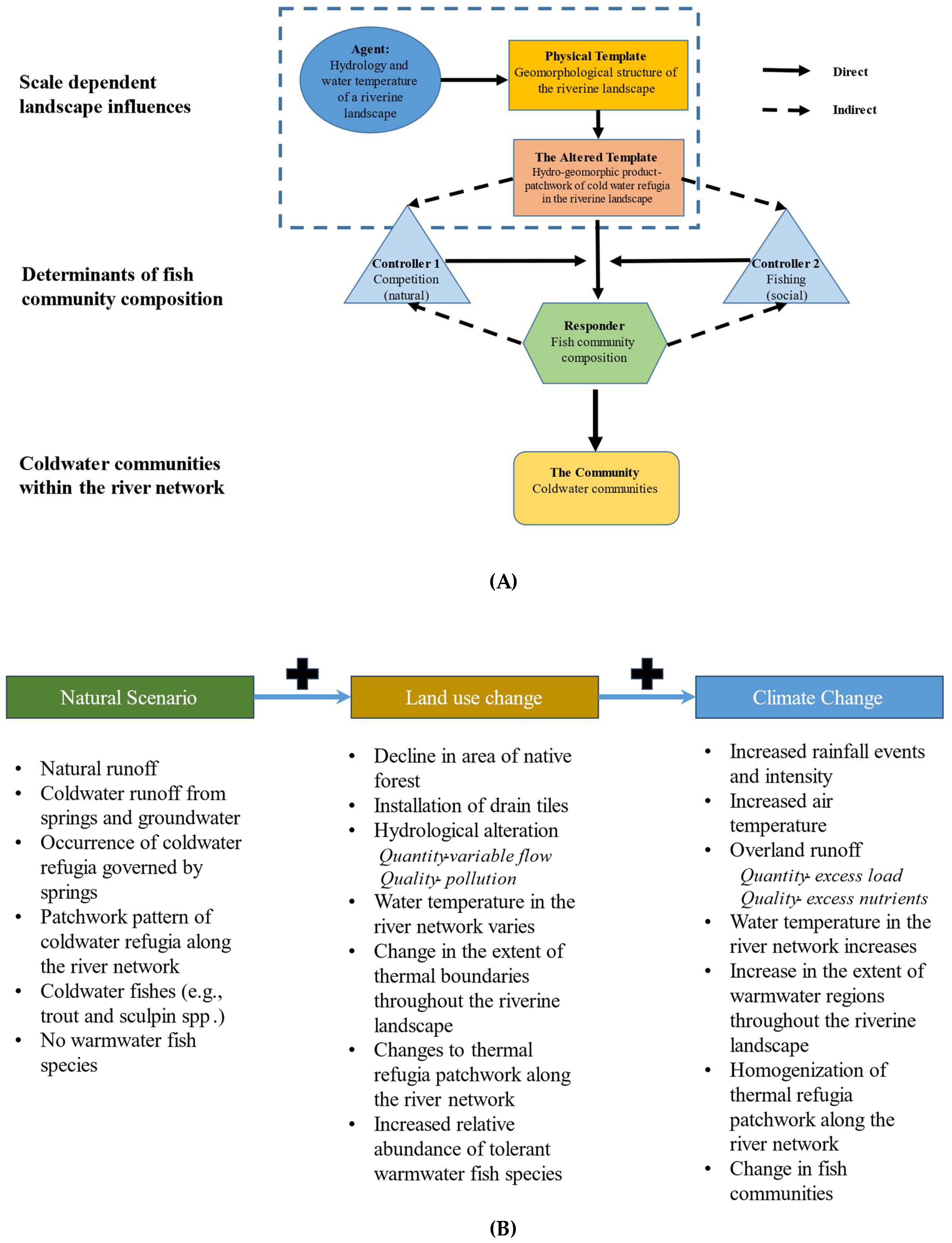

Table 1.
Spring data showing distribution and influence of inputs for both flow in liters/sec (Q) and mean temperature (x-bar). Abbreviations are North Fork (NF), Middle Fork (MF), South Fork (SF), headwaters (HW), middle sections (MS), and lower sections (LS) of each fork. Means (x-bar) for variable are shown with + one standard deviation. Chi-square results testing for differences distribution among forks and differences in pattern among sections. Asterisks denote significance and number of asterisks denote strength. Data collected from the Minnesota Spring Inventory website for spring located in the Whitewater catchment in southeastern Minnesota, USA. .
| Springs | Testing | |||||||
| Fork | x̄ | Q | n | X2 | DF | P | ||
| North | 9.2 (3.04) | 459 | 26 | |||||
| Middle | 9.6 (3.10) | 3,978 | 30 | 9.3 | 2 | 0.05* | ||
| South | 9 (3.00) | 1,854 | 19 | |||||
| Section | ||||||||
| NF- HW | 9.9 | 28 | 1 | |||||
| NF- MS | 1 | 41.1 | 2 | < 0.0001** | ||||
| NF- LS | 9.2 | 431 | 24 | |||||
| MF- HW | 8.9 | 184 | 3 | |||||
| MF- MS | 12.6 | 305 | 7 | 15.8 | 2 | < 0.0001** | ||
| MF- LS | 8.7 | 3489 | 20 | |||||
| SF- HW | 9.1 | |||||||
| SF- MS | 1 | 32.5 | 2 | < 0.0001** | ||||
| SF- LS | 9 | 1854 | 18 | |||||
Table 2.
Results from linear model with diversity used as the response and river.km as the predictor. Shown are model estimate, standard error, r-square value, T and F statistic, and probability statistic. Asterisk denotes significant differences and strength. Data represented is for the three forks (North, Middle, South) of the Whitewater River located in southeastern Minnesota, USA.
| Coefficient | Estimate | Std. Error | T | P |
| Middle Fork | 0.486 | 0.064 | 7.55 | 3.9e-10*** |
| North Fork | 0.151 | 0.077 | 1.96 | 0.05 |
| South Fork | 0.283 | 0.081 | 3.51 | 0.001*** |
| River.km | -0.001 | 0.002 | -0.499 | 0.62 |
| Model | R2 | DF | F | P |
| lm | 0.16 | 3 and 57 | 4.72 | 0.005 |
Table 3.
Fish community SDI values obtained for each fork by section. Abbreviations are as follow, North Fork (NF), Middle Fork (MF), South Fork (SF), headwater (HW), middle section (MS), and lower section (LS). X-bar is the mean value for SDI. All values are 1-D. ANOVA results are shown with f-statistic and p-value. Asterisk denotes significant differences. Data represented is for the three forks (North, Middle, South) of the Whitewater River located in southeastern Minnesota, USA.
| Fork | x̄ | F | P |
| NF- HW | 0.49 (0.35) | ||
| NF- MS | 0.67 (0.05) | 1.52 | 0.245 |
| NF- LS | 0.60 (0.15) | ||
| MF- HW | 0.61 (0.27) | ||
| MF- MS | 0.72 (0.02) | 6.71 | 0.007* |
| MF- LS | 0.29 (0.24) | ||
| SF- HW | 0.59 (0.24) | ||
| SF- MS | 0.79 (0.05) | 3.35 | 0.05* |
| SF- LS | 0.73 (0.12) |
Table 4.
Mean (+ one standard deviation) CPUE (trout/min) and abundance (fish/km) of trout. Abbreviations are as follow: North Fork (NF), Middle Fork (MF), South Fork (SF), headwaters (HW), middle sections (MS), and lower sections (LS). ANOVA results are shown with f-statistic and p-value. Asterisk denotes significant differences. Data collected during late spring and early fall in 2018 and 2019 in the Whitewater River catchment in southeastern Minnesota, USA.
| Fork | CPUE | Abundance | F | P | ||
| NF - HW | 0.043 (0.07) | 32 (0) | ||||
| NF - MS | 0.23 (0.15) | 82 (33.4) | 9.21563 | 0.00322* | ||
| NF - LS | 0.56 (0.24) | 193 (82.3) | ||||
| MF - HW | 0.202 (0.21) | 67 (63.9) | ||||
| MF - MS | 0.62 (0.70) | 166 (204) | 3.19866 | 0.06966 | ||
| MF - LS | 1.30 (0.96) | 338 (216) | ||||
| SF - HW | 0.01 (0.01) | 11 (0) | ||||
| SF - MS | 0.23 (0.15) | 65 (34) | 16.5381 | 0.00016* | ||
| SF - LS | 0.73 (0.15) | 234 (97) | ||||
| Model | F | DF | P | |||
| lm | 14.72 | 5 and 55 | 3.75e-09*** |
Table 5.
Linear model testing of trout condition. Estimate value is the model response, standard error, t-statistic of testing, and the probability statistic. Model outputs are adjusted r-square, degrees of freedom, F statistic, and model p-value. Asterisks denote significance and strength. Data collected during late spring and early fall in 2018 and 2019 in the Whitewater River catchment in southeastern Minnesota, USA.
| Fork | Estimate | Std. Error | T | P |
| Middle | 83.9 | 2.53 | 33.14 | 2e-16 *** |
| North | -7.66 | 2.88 | -2.65 | 0.0121 * |
| South | -11.2 | 3.48 | -3.21 | 0.0029 ** |
| River.km | 0.5 | 0.09 | 5.03 | 1.69e-05 *** |
| Model | R2 | DF | F | P |
| Lm | 0.38 | 3 and 33 | 8.303 | 0.0003 |
Table 6.
Mean (+ one standard deviation) trout condition (relative weight, Wr) within sections of each fork. Abbreviations are as follow: North Fork (NF), Middle Fork (MF), South Fork (SF), headwaters (HW), middle sections (MS), and lower sections (LS). Also shown are ANOVA results with f and p-value. Asterisk denotes significant differences. Data collected during late spring and early fall in 2018 and 2019 in the Whitewater River catchment in southeastern Minnesota, USA.
| Fork | Wr | F | P |
| NF-HW | 110 (0.90) | ||
| NF-MS | 89 (7.41) | 11.2301 | 0.00277* |
| NF-LS | 85 (3.97) | ||
| MF-HW | 93 (5.50) | ||
| MF-MS | 96 (6.31) | 1.04063 | 0.38556 |
| MF-LS | 91 (5.90) | ||
| SF-HW | 118 (0) | ||
| SF-MS | 90 (6.32) | 10.0172 | 0.00883* |
| SF-LS | 86 (5.64) |
Table 7.
Canonical variates produced by modeling with stream (X) and catch statistic variables (Y) using Canonical Correlations. Results show correlation strength (Corr) between the variate pair, approximate F-test statistics, and p-values for tests of non-zero correlations. Data collected during late spring and early fall in 2018 and 2019 in the Whitewater River catchment in southeastern Minnesota, USA.
| Variate | Corr | F | P |
|---|---|---|---|
| 1 | 0.764 | 5.45 | 9.63E-06 |
| 2 | 0.510 | 2.97 | 0.026 |
| 3 | 0.196 | 1.32 | 0.259 |
Disclaimer/Publisher’s Note: The statements, opinions and data contained in all publications are solely those of the individual author(s) and contributor(s) and not of MDPI and/or the editor(s). MDPI and/or the editor(s) disclaim responsibility for any injury to people or property resulting from any ideas, methods, instructions or products referred to in the content. |
© 2024 by the authors. Licensee MDPI, Basel, Switzerland. This article is an open access article distributed under the terms and conditions of the Creative Commons Attribution (CC BY) license (http://creativecommons.org/licenses/by/4.0/).
Copyright: This open access article is published under a Creative Commons CC BY 4.0 license, which permit the free download, distribution, and reuse, provided that the author and preprint are cited in any reuse.


