Submitted:
20 June 2024
Posted:
21 June 2024
Read the latest preprint version here
Abstract
Short-term energy consumption forecasting crucial for the operation of new electrical en-ergy grids, not only due to their own characteristics, but also due to the new elements pre-sent in the energy matrix. Many existing models are limited by their methodologies or by considering only a narrow set of factors influencing energy consumption. This study in-troduces a pipeline for developing an energy forecasting model and evaluates the signifi-cance of factors affecting energy consumption and, consequently, forecast accuracy. The study utilizes a dataset from ISO NE (Independent System Operator New England), span-ning the total electric load of various cities in New England from January 2017 to December 2019. This dataset comprises 23 independent variables, including weather data, economic indicators, and market information. The results outline the steps involved in constructing energy forecast models using time series analysis. By carefully selecting variables and rep-resenting external factors, the study demonstrates the feasibility of generating more accu-rate predictions with reduced computational resources.
Keywords:
electricity forecasting model
; deep learning
; computational intelligence
1. Introduction
The traditional structure of the Electric Power System is characterized by the presence of large power generation plants (such as hydroelectric and thermal power plants) located far from the consumption areas. In this kind of system, decisions are centralized and the flow of energy is unidirectional, meaning it goes from the operators to the end consumers.
Changes in the energy matrix, driven by a growing proportion of clean and sustainable sources and spurred by the deregulation of the sector, are reshaping the terrain of electric power grid management. We are moving from a scenario with stable predictions and controlled power generation to a more volatile and less predictable scenario, where the flow of energy is bidirectional, traversing from operators to consumers and vice versa [1].
Modern electric grids, referred to as "Smart Grids," represent an evolution designed to address contemporary challenges by leveraging advanced communication and information technologies. These grids encompass not only the transmission of energy from generation to substations but also the distribution of electricity from substations to individual end-users [2].
In this new networks, electrical load forecasting and energy generation forecasting play fundamental roles in maintaining network stability, preventing overloads and to ensure a smooth transition to more ecologically sustainable energy use, all depending on the ability to understand and predict energy supply and demand [3].
To predict energy generation, the procedure proposed in [4] can be utilized. For predicting electrical load demand, the pipeline developed in this study is applicable. The sparse interconnection of alternative energy sources and the loads they supply necessitates distributed control and monitoring of energy flow. Distributed control needs higher availability of information for effective decision-making [5]. Decision-making could be of two types: a) involving unit commitments with response times of several hours and b) load dispatch decisions with response times ranging from a few minutes to several hours [6]. The pipeline proposed in this study primarily aims to address load dispatch, so the focus is on suitable methods for short-term electric energy prediction.
The main contributions of this paper can be summarized as follows: (1) Emphasizing the growing significance of short-term energy consumption prediction; (2) Offering a comprehensive framework detailing the construction of energy prediction models; (3) Addressing critical considerations in the development of energy consumption prediction models; (4) Evaluating model effectiveness through the analysis of its representation of consumption-affecting factors and the efficacy of relevant prediction methodologies.
The remainder of this paper is organized as follows: Section 2 elaborates on the applicable techniques, implementation challenges, and the proposed prediction model pipeline, while Section 3 outlines the conducted experiments and their results. The concluding section presents the study's findings, followed by the inclusion of bibliographic references.
2. Energy Prediction
2.1. Energy Consumption
Electric energy consumption is subject to a multitude of influencing factors, including user behaviors, weather conditions, seasonal variations, economic indicators, and more [7]. The nonlinear nature of the relationship between exogenous factors and energy consumption add complexity to energy prediction processes.
The complexities of energy prediction stem from the granularity of the demand being forecasted. Predicting aggregate consumer demand proves to be more manageable than individual consumer demand due to stronger correlations with external factors like temperature, humidity, and internal factors such as historical trends. Aggregation mitigates the inherent volatility of individual consumers, resulting in a smoother curve shape and greater homogeneity [8].
In [9] the two situations are compared, one where the prediction of individual users is made and the aggregate prediction is generated from them and another where the prediction of the electrical load is made directly from the aggregate demand.
With regard to reducing energy consumption, it is important to take into account the use of strategies to control the temperature of buildings and reduce costs by taking advantage of surplus photovoltaic energy, as proposed in [10].
2.2. Selection of the prediction method
2.2.1. Prediction Technique based on time series
One of the possible ways to predict energy consumption is through time series analysis. Time series data allows for predicting future values based on past values with a certain margin of error [11].
Traditional techniques for energy demand prediction encompass statistical time series models, such as ARIMA (autoregressive integrated moving average), SARIMA (seasonal ARIMA), and exponential smoothing. For [12], these techniques are benchmarks in the field of energy demand forecasting.
In recent decades, however, computational intelligence methods have gained prominence for better describing the trends of nonlinear systems and taking into account the effects of exogenous factors. As examples, we can mention, according to the same author, the Artificial Neural Network (ANN), the Support Vector Machine (SVM) and others.
Recent works published in the last five years indicate a growing adoption of deep learning techniques for several reasons, including their potential to generate more accurate predictions, advancements in processing capabilities, and the greater availability of information (large datasets). Examples of these techniques include Long Short-Term Memory (LSTM), Convolutional Neural Network (CNN), as well as combinations thereof. As previously mentioned, while they offer more accurate predictions, they also entail higher computational costs [9,14,15,16].
2.2.2. Deep learning techniques
According to [13], “neural networks represent a subfield of machine learning and deep learning constitutes a subfield of neural networks that has revolutionized various fields of knowledge in recent decades.”. Deep learning employs deep architectures or hierarchical learning methods consisting of multiple layers between the input and output layers, followed by various stages of non-linear processing units. These models are attractive because it explores well the learning characteristics and classifying patterns [17]. Since deep learning was introduced, some disruptive solutions have been developed, showcasing its success in various application domains. Below, the characteristics of the deep learning techniques considered in the study are briefly described.
Artificial Neural Networks (ANNs), or general neural networks, consist of a perceptron that contains few or no internal layers with multiple units (neurons). A Dense Neural Network (DNN) is a perceptron with multiple internal layers capable of modeling complex nonlinear relationships with fewer processing units compared to the general neural network while achieving similar performance.
A Recurrent Neural Network (RNN) is fundamentally different from a conventional neural network because it is a sequence-based model that establishes a relationship between previous information and the current moment. This means that a decision made by the RNN at the current time can impact future time steps.
As a successful RNN model, LSTM (Long Short Term Memory) presents a cell memory that can retain its state over time and non-linear gate units to control the flow of information into and out of the cell [17]. Figure 1 illustrates these elements.
The operations performed by the elements identified in the previous figure are represented by the equations below [18].
where Wi, Wf, Wo, e bi, bf, bo are the weights and biases that govern the behavior of the it (input gate), ft (forget gate) e ot (output gate), respectively, and where Wc and bc are the weights and bias of the (memory cell candidate) and Ct is the cell state. Consider that xt is the input to the network, ht is the output of the hidden layer and σ denotes the sigmoidal function.
ft = σ (Wf × [ht−1, xt] + bf),
it = σ(Wi × [ht−1, xt] + bi),
ot = σ(Wo × [ht−1, xt] + bo),
ht = ot × tanh(Ct),
A Convolutional Neural Network (CNN) is a particular type of neural network that also acts as a feature extractor [17]. This neural network utilizes a combination of convolution and pooling layers applied to input data to extract new features. These features are then used as new inputs and passed to a classic MLP neural network, also known as a fully connected layer. Convolution involves extracting feature maps from each input using a filter with a specific size (typically square filters) and a stride (a left-to-right and top-to-bottom step). The feature maps extracted by the filters (kernels) are subsequently smaller than the input matrix and have different values since each filter is distinct. The feature maps are then used as inputs for the next layer, which can be another convolution layer or a pooling layer; a pooling layer shortens the feature map using a filter with a specific size and stride and the reduction performed by the pooling layer can be either max pooling or average pooling.
After the convolution and pooling layers, the extracted feature maps are flattened and passed to a fully connected layer, as indicated in Figure 2.
The hybrid model that combines a CNN and an LSTM represents an alternative to enhance prediction accuracy and stability by leveraging the advantages of each. The CNN preprocesses the data and extracts features from the variables that affect consumption, while the LSTM handles modeling temporal information with irregular trends in the time series and uses this information for future estimates. In some situations, a model that employs a single machine learning algorithm may not have as much complexity, but its results can be unrealistic and imprecise [13,15].
2.3. External factors
External factors that affect energy consumption, as mentioned in Section 3.1, are represented by adding or generating new variables derived from the combination of available variables.
2.3.1. Cyclical seasonality
It's intuitive to envision energy consumption curves displaying annual, weekly, and daily cyclic variations. Across the year, consumption fluctuates with the changing seasons. Weekly variations arise from differing consumption patterns on weekdays versus weekends. Similarly, consumption experiences daily fluctuations, often peaking when individuals return home from work.
To replicate these phenomena, [20] introduced several encoding techniques such as binary encoding, linear relationships, and trigonometric functions. These encoding methods serve to distinguish between days of the week and hours of the day, thereby capturing weekly and daily seasonal behaviors. In [21], all these approaches were evaluated, with optimal outcomes observed when using day of the week (dc) coding set to 3, equivalent to employing a 7-bit coding scheme, and time of day (hc) coding set to 2, corresponding to the utilization of trigonometric functions.
2.3.2. Calendar
Energy consumption is influenced by the calendar, which establishes holidays, workdays and weekends [12]. Additionally, the calendar allows us to identify the working hours during which consumption is higher.
Holidays exhibit an atypical behavior in terms of both daily energy consumption and the duration of the consumption curve. The reference for energy consumption on a holiday is the value consumed on the same day of the previous year. For some holiday dates, it is also necessary to consider the induced holiday, which is the bridge day between the holiday and the next weekend. On these days, energy consumption is lower than on workdays.
2.3.3. Thermal discomfort index
According to [23], buildings are responsible for 30% of global final energy consumption and 26% of global energy-related emissions. A significant portion of this energy is used to ensure the thermal comfort of the facilities. Thermal discomfort is related to the field of building ambience studies, which aims to design people's well-being, meaning to provide a bodily state in which there is no sensation of cold or heat. Figure 3 illustrates the boundaries of a thermal comfort zone.
Within the survival zone, one can discern the temperature thresholds crucial for human survival. These limits encompass hypothermia, characterized by a body temperature below 35 °C, and hyperthermia, denoting a significant rise in body temperature. At the outermost edges of the thermal comfort zone lie the critical temperatures, divided into lower and upper categories.
Figure 3.
Thermal Comfort Zone.m (Source: [26]).
Figure 3.
Thermal Comfort Zone.m (Source: [26]).

The method used to obtain the thermal discomfort index is based on the formula adapted by [24] and cited by [25]. In this formula, Ta represents the air temperature in degrees Celsius (°C) and To represents the dew point temperature, also in degrees Celsius (°C).
where:
Id = 0,99 × Ta + 0,36 × To + 41,5,
Id - Discomfort Index
Ta - Ambient temperature
To - Dew point temperature
The thermal comfort condition is determined by referencing Table 1, as presented by [26], which provides the calculated discomfort index (Id).
When Id values fall within the extreme ranges, exceeding 75 or dropping below 60, individuals tend to activate air conditioning devices.
2.3.4. Market and economic indicators
Econometric models indicate that Gross Domestic Product (GDP), energy prices, gross production and population influence energy consumption [27].
2.4. Modeling methodology
Essentially, the models utilized in electric prediction employing computational intelligence can be categorized into two types: one treats consumption data purely as a time series, with the impact of exogenous factors implicitly embedded within the data, making it univariate. The other type is multivariate, explicitly incorporating all factors influencing consumption into the model.
Regarding the prediction horizon, the model can be either one-step or multi-step, allowing the user to specify how many time steps ahead they wish to forecast demand.
For [28], building neural network models is more like an art than a science, as there is a lack of a clear methodology for parameter determination. The author highlights the challenge in this domain as developing a systematic approach to assembling a suitable neural network model for the specific problem at hand.
2.4.1. Pipeline for creating energy prediction models
Constructing a neural network prediction model for a specific problem is not a trivial task. According to [29], a critical decision is determining the appropriate architecture. While there are tools that assist in this task, parameter selection also depends on the problem and/or the information available in the dataset.
A forecast of a county’s energy demand, for example, may rely on the recent history of demand (endogenous factors) as well as weather forecasts, which are exogenous factors. Many time series methods, such as autoregression with exogenous variables (ARX), have extensions that accommodate these variables. However, it is often necessary to prepare the exogenous data before use, ensuring it matches the temporal resolution of the variable being forecast (e.g., hourly, daily) [30].
The creation of models is complicated by the numerous choices that must be made prior to defining the model itself. Consequently, designers often face uncertainty regarding the decisions to be made. Therefore, instead of an exhaustive exploration of the subject, the main goal here is to provide support to streamline the process of creating load prediction models.
It is worth noting that the most accurate models are the ones that capture the behavior of input variables and replicate their impact on the output. Therefore, it is important to develop an understanding of which factors are most relevant to the problem and how to represent them in the model.
To identify these factors, questions related to the problem and the chosen prediction techniques were considered [31].
- a)
- Questions related to prediction techniques
-
How many neurons should the input layer have?The number of input nodes or neurons is probably the most critical decision for time series-based modeling since it defines which information is most important for the complex non-linear relationship between inputs and outputs. The number of input neurons should match the number of relevant variables for the problem [29].
-
How many hidden layers should the model have?As emphasized by [29], a network with no hidden layers represents a model with linear outputs, equivalent to linear statistical prediction models. Some authors, such as [32], suggest that typically no more than two hidden layers are necessary in a network to effectively address most prediction problems.This study assess two architectures: one shallow and the other deep. They vary in the number of intermediate layers, with the the deep model incorporating additional intermediate layers. The specific attributes of shallow and deep models are detailed in Appendix A.
-
How many neurons should the hidden layers have?According to [33], an excessive number of neurons per hidden layer can degrade model generalization and lead to overfitting. Therefore, it is suggested that the number of hidden nodes should be correlated with the number of inputs. The following expression was proposed to define it:where n is the number of input variables and Nh is the number of neurons in the intermediate layers. According to [17], a deep neural network allows you to model complex data with fewer processing units compared to a conventional neural network with similar performance.Nh = (4n2 + 3)/(n2 – 8),
-
What hyperparameters to use and how to select them?Hyperparameters are attributes that control machine learning model training. Deep neural network models have several hyperparameters. The strategy used to define them was to process the model using GridsearchCV from Sklearn [34]. By processing the dataset with GridsearchCV, the best parameter adjustments were identified. Refer to Appendix B for further details.
-
Which training algorithm to use?Training a neural network entails minimizing a non-linear function, adjusting the network's weights to minimize the total mean squared error between desired and actual values. The backpropagation algorithm, a gradient descent algorithm, is widely utilized for this purpose [29]. In this method, the magnitude of each step is referred to as the learning rate. A small learning rate typically results in slow learning, whereas a high learning rate may induce network oscillation. The standard backpropagation technique is favored by most researchers, as it supports both online and batch updates.
-
Which prediction algorithm to use?As mentioned in Section 3.2, deep learning techniques are the most promising for demand prediction applications. Therefore, they were prioritized in this study.
-
How many output nodes to use?The number of output nodes is relatively easy to specify because it is related to the problem under study. For a time series-based problem, the number of output nodes corresponds to the number of time intervals ahead that you want to predict [29].
- b)
- Questions related to problem
-
Why preprocess the data?Data cleaning is necessary whenever outliers or out-of-pattern data are identified. Normalization is important because it ensures that all input data for the model has the same weight and range of variation [35].
-
Which input variables to consider?Some variables are dominant compared to others and need to be prioritized for inclusion in the model. To select them, algorithms that quantify the correlation between these variables and the target variable were used. Examples of these algorithms are available in the open-source software package Waikato Environment for Knowledge Analysis (WEKA). It should be noted that the selection of input variables affects the training speed and the model's response [36].
-
How to reproduce seasonality?
-
How to consider the calendar?The calendar allows differentiating, from the perspective of energy consumption, holidays, workdays and hours of work throughout the day when energy consumption changes. The coding used is shown in Table 2.
-
How to represent the discomfort index?The discomfort index is important because it indicates the user's predisposition to turn on the air conditioning or other climate control equipment in their environment, which can be energy-consuming. It is calculated as indicated in Section 3.3
Based on the previous analyses, it was possible to define the essential steps required for constructing more precise and well-fitted prediction models. This is illustrated in the pipeline depicted in Figure 4.
Finally, to measure the accuracy of the models (Evaluate Error block), several metrics can be employed. In this study, we use the Mean Absolute Percentage Error (MAPE) metric, a widely accepted measure of prediction accuracy in time series analysis. MAPE is calculated by taking the average of the absolute percentage errors between the predicted and actual values. This metric is particularly useful because it expresses the error as a percentage, making it easier to interpret the model's performance across different scales and datasets. It is is determined by:
where, n represents the number of observed instances, is the current consumption value and is the predicted value for each point. It shows that the total absolute error value is determined by summing up the absolute values of each instance divided by the number of evaluated points, n. The conclusions are based on MAPE values, where a lower MAPE value indicates higher model accuracy [19].
3. Implementation and results
The subsequent discussion and analysis are anchored in the initial premise that constructing an energy consumption forecast model is inherently complex, primarily due to the multitude of decision-making processes involved.
To enhance clarity in comprehending the construction of load prediction models, a structured pipeline has been introduced. This pipeline encompasses the stages essential for developing multivariate and multistep models utilizing deep learning techniques. Each stage is meticulously justified, emphasizing its necessity and specific contribution.
Thus, what follows is a systematic evaluation of the fundamental components essential to composing accurate load forecasting models. To demonstrate the pipeline's applicability and evaluate its efficacy, a comprehensive array of experiments has been conducted. These experiments encompass various input conditions (number of variables) and output conditions (time horizon), as detailed in the subsequent tables. Notably, they encompass different configurations of input variables, prediction algorithms, and model architectures (shallow or deep).
3.1. Dataset
The dataset used in this study can be accessed on the ISO NE (Independent System Operator New England) website at http://www.iso-ne.com. It includes the total electric load of several cities in England for a period between January 2017 and December 2019 and comprises 23 independent variables of the following nature: weather information, economic indicators and market data.
Graphical representations displaying annual, weekly, and daily variations in total energy consumption for the aforementioned dataset are available in [22]. The Annual Variation chart reveals peaks during the summer months and another, albeit less intense, peak in the winter months. The Weekly Variation chart illustrates higher consumption levels on Mondays, while the Daily Variation chart depicts consumption peaks during the day, particularly between 6 and 7 pm.
3.2. Experiments
The conducted experiments are summarized in Table 3, Table 4, Table 5 and Table 6, encompassing various combinations of input variables, algorithms, and prediction horizons. The implementation was carried out using the Python programming language along with machine learning libraries, Sklearn and Keras [34]. In order to underscore the significance of step (1) of the pipeline, experiments detailed in Table 3 were conducted, focusing on variations in input variables and comparing processing times.
It is important to highlight that the processing detailed in Table 3 includes seasonality and calendar representation. Additionally, it's noteworthy that the variable selection algorithms employed originate either from the Weka tool or were custom-built in Python (refer to the source column). The experimental results were compared based on precision (MAPE) and processing time (refer to the magnitudes column).

Table 3.
Experiments with Variation in Input Variables (Horizon: One Step Ahead).
| Technique | Source | Selected variables | Magnitudes | Dnn | Cnn | Lstm | Cnn+Lstm | ||||
|---|---|---|---|---|---|---|---|---|---|---|---|
| Shallow | Deep | Shallow | Deep | Shallow | Deep | Shallow | Deep | ||||
| Cfs Subset Evail | Weka |
RT demand, DACC, DA MLC, RT MLC, MIN_5MIN_RSP, MAX_5MIN_RSP |
Mape | 0,22 | 0,18 | 1,8 | 0,74 | 0,37 | 0,24 | 0,21 | 0,18 |
| t(s) | 152 | 185 | 276 | 340 | 887 | 1798 | 739 | 848 | |||
| Classifier atribute Evail | MAX_5MIN_RSP, DA EC, DA CC, RT demand, DA LMP | Mape | 0,27 | 0,23 | 1,6 | 0,48 | 0,21 | 0,16 | 0,26 | 0,24 | |
| t(s) | 153 | 187 | 342 | 384 | 994 | 1813 | 761 | 790 | |||
| Principal Componentes | RT LMP, RT EC, DA LMP, DA EC, RT MLC | Mape | 7,8 | 6,84 | 9,67 | 6,5 | 10,95 | 9,79 | 8,06 | 7,57 | |
| t(s) | 87 | 130 | 150 | 219 | 594 | 912 | 996 | 386 | |||
| Relief | RT demand, DA demand, DA EC, DA LMC, Reg Service Price | Mape | 0,52 | 0,33 | 3,82 | 0,22 | 0,23 | 0,16 | 0,16 | 0,17 | |
| t(s) | 112,8 | 123 | 274 | 339 | 906 | 1792 | 692 | 823 | |||
| Mutual information | Python | DA MLC, DA LMP, MIN_5MIN_RSP, DA EC, Dew Point | Mape | 5,9 | 5,76 | 8,15 | 5,03 | 10,21 | 7,82 | 7,23 | 6,11 |
| t(s) | 155 | 186 | 270 | 339 | 581 | 1827 | 725 | 792 | |||
| - | - | All | Mape | 0,86 | 0,38 | 2,27 | 1,05 | 0,29 | 0,2 | 0,25 | 0,20 |
| t(s) | 118 | 123 | 158 | 153 | 591 | 920 | 695 | 879 | |||
Source: Author.
Based on these experiments, the following observations can be made:
- ○
- Among the tested variable selection algorithms, notable ones include CFS Subset Eval, Classifier Attribute Eval, and Relief. These algorithms selected the 5 or 6 variables most correlated with the target variable, yielding predictions with error rates similar to or lower than those obtained when considering all variables in the database (as indicated in the last line of Table 3). This underscores the relevance of the selected variables.
- ○
- Regarding the performance of models with different prediction algorithms, LSTM stands out for requiring the highest computational cost. It necessitates 10 times more processing time than DNN, 5 times more than CNN, and 2.5 times more than the combined CNN+LSTM model. However, the models employing LSTM and a combination of CNN+LSTM achieved the highest accuracy.
- ○
- Comparing the performance of shallow and deep models, it was observed that the latter incur a higher computational cost. Nevertheless, in most scenarios, they demonstrate superior accuracy compared to shallow models.
To demonstrate the importance of integrating external factors into the model, as outlined in step (2) of the pipeline, some experiments were conducted, and their results are presented in Table 4 and Table 5.
In these tables, the columns indicate the presence of external factors, with the distinction based on the prediction horizon. The acronyms and elements included in the columns are defined as follows: Sh-Shallow; D-Deep; Sl-System Load; W-Weather; S-Sazonality; Fs-Feature Selection; Av-All Variable, Id-Discomfort index, Δ- Percentage variation of error. For instance, the column Sl+W presents the results incorporating both System Load and Sazonality external factors for different prediction algorithms.
Table 4.
MAPE of Processes with Different Sets of Input Variables.
| Horizon: One step ahead | |||||||||||
|---|---|---|---|---|---|---|---|---|---|---|---|
| Technique | Model | Sl (1) | Sl+W (2) | Sl+S+C+Id (3) | Δ(%) (4) | Fs (5) | Fs+S+C+Id (6) | Δ(%) (7) | Av (8) | Av+S+C+Id (9) | Δ(%) (10) |
| Dnn | Sh | 11,3 | 6,76 | 5,38 | 52,4 | 0,29 | 0,19 | 34,5 | 0,19 | 0,18 | 5,3 |
| D | 10,85 | 5,98 | 8,57 | 44,9 | 0,37 | 0,17 | 54,1 | 0,22 | 0,17 | 22,7 | |
| Cnn | Sh | 12,13 | 8,46 | 8,0 | 34 | 2,85 | 2,23 | 21,8 | 3,40 | 2,26 | 33,5 |
| D | 11,04 | 4,95 | 4,29 | 61,1 | 0,18 | 0,18 | 0 | 0,26 | 0,16 | 38,5 | |
| Lstm | Sh | 12,37 | 8,31 | 7,86 | 36,5 | 0,65 | 0,25 | 61,5 | 0,47 | 0,17 | 63,8 |
| D | 11,74 | 7,59 | 9,0 | 23,3 | 14,1 | 7,07 | 49,8 | 14,96 | 10,45 | 30,1 | |
| Cnn+Lstm | Sh | 10,38 | 6,56 | 5,67 | 45,4 | 0,31 | 0,21 | 32,2 | 0,42 | 0,19 | 54,8 |
| D | 11,11 | 5,09 | 7,60 | 31,6 | 0,25 | 0,15 | 40 | 0,25 | 0,24 | 4 | |
Source: Author.
Table 5.
MAPE of Processes with Different Sets of Input Variables.
| Horizon: Twelve step ahead | |||||||||||
|---|---|---|---|---|---|---|---|---|---|---|---|
| Technics | Model | Sl (1) | Sl+W (2) | Sl+S+C+Id (3) | Δ(%) (4) | Fs (5) | Fs+S+C+Id (6) | Δ(%) (7) | Av (8) | Av+S+C+Id (9) | Δ(%) (10) |
| Dnn | Sh | 33,2 | 23,44 | 27,98 | 15,7 | 36,58 | 29,77 | 18,6 | 29,8 | 29,76 | 0,13 |
| D | 48,1 | 27,63 | 37,01 | 23,1 | 45,03 | 32,4 | 28,1 | 44,0 | 40,58 | 7,77 | |
| Cnn | Sh | 12,01 | 15,37 | 4,92 | 59,0 | 4,91 | 4,83 | 1,6 | 4,92 | 4,68 | 4,9 |
| D | 10,6 | 9,19 | 3,77 | 64,4 | 4,79 | 3,96 | 17,3 | 4,39 | 3,63 | 17,7 | |
| Lstm | Sh | 13,00 | 14,36 | 9,82 | 24,5 | 4,39 | 4,30 | 2,0 | 4,29 | 3,66 | 14,7 |
| D | 15,58 | 15,65 | 15,27 | 2,0 | 15,8 | 11,34 | 4,46 | 15,4 | 15,15 | 1,62 | |
| Cnn+Lstm | Sh | 15,00 | 8,04 | 4,58 | 69,5 | 4,42 | 3,93 | 11,0 | 4,12 | 4,09 | 0,7 |
| D | 11,24 | 8,65 | 10,7 | 4,8 | 15,94 | 10,82 | 32,1 | 15,6 | 15,36 | 1,5 | |
Source: Author.
Considering the experiments detailed in Table 4 and Table 5, the following observations can be made:
- ○
- The distinguishing factor between the tables is the prediction horizon. It is evident that increasing the prediction horizon leads to a reduction in accuracy.
- ○
- Experiments involving only the target variable (Sl), with or without external factors, exhibited the highest errors. This implies that deep learning algorithms face limitations in their generalization capacity when operating with a very limited number of input variables, resulting in elevated error rates.
- ○
- Comparing predictions based on only the target variable (Sl), the selected variables (Fs), and all variables in the dataset (Av), it is notable that errors in the Fs and Av columns are closely aligned. This suggests that despite variable selection reducing the number of input variables from 23 to 6 or 7, this reduction did not lead to an increase in prediction errors.
To evaluate the impact of architecture on the model's performance, experiments detailed in Table 6 were carried out. These experiments varied the number of intermediate layers and neurons within those layers. Deep learning models were employed, and variable selection was conducted using the Weka Classifier Attribute Eval. Additionally, the inclusion of external factors such as seasonality and calendar was taken into account during the experiments.
Table 6.
Experiments with deep models varying the number of intermediate layers and neurons per intermediate layer (MAPE values for one-step-ahead prediction).
Table 6.
Experiments with deep models varying the number of intermediate layers and neurons per intermediate layer (MAPE values for one-step-ahead prediction).
| DNN | CNN | LSTM | CNN+LSTM | ||||||||||
| Number of neurons | Number of neurons | Number of neurons | Number of neurons | ||||||||||
| 6 | 15 | 32 | 6 | 15 | 32 | 6 | 15 | 32 | 6 | 15 | 32 | ||
| Number of intermediate layers | 2 | 0,24 | 0,15 | 0,41 | 0,18 | 0,15 | 0,15 | 0,23 | 0,16 | 0,19 | 0,3 | 0,15 | 0,25 |
| 3 | 0,3 | 0,54 | 0,16 | 0,15 | 0,26 | 0,29 | 0,52 | 0,15 | 0,17 | 0,18 | 0,43 | 0,52 | |
| 4 | 0,17 | 0,44 | 0,2 | 0,19 | 0,18 | 0,17 | 2,34 | 0,46 | 0,81 | 0,18 | 0,17 | 0,17 | |
| 6 | 0,24 | 0,15 | 0,16 | 0,3 | 0,18 | 0,41 | 10,0 | 15,4 | 0,40 | 15,53 | 0,40 | 0,35 | |
Source: Author.
From the point of view of the model structure, Table 6 suggests that utilizing two or three intermediate layers with a recommended number of neurons equal to 6 (Eq. (8)) enables the generation of predictions with lower computational cost and error rates within an acceptable range (<1%).
In summary, the conducted experiments allow for several conclusions:
- ○
- Multivariate and multistep models offer flexibility by permitting variations in the number of input variables and prediction intervals, making them appealing for energy consumption forecasts.
- ○
- It has been demonstrated that incorporating external factors enhances model accuracy, with experiments achieving up to a 60% increase in accuracy.
- ○
- It has been proven that incorporating external factors increases the accuracy of the model, with experiments achieving an accuracy increase of up to 60%.
- ○
- Variable selection is a necessary measure when the number of input variables is large. It enables the reduction of the problem's dimensionality while still achieving good accuracy through the model. This reduction in dimensionality promotes the application of deep learning techniques and the utilization of deep models.
- ○
- In deep learning models, defining the architecture is a crucial step. The experiments have demonstrated that it's unnecessary to incorporate more than three intermediate layers or introduce an excessive number of neurons within these layers. It has been proven that adhering to the number of neurons defined by Eq. (8) yields satisfactory results.
- ○
- From the perspective of model accuracy, it's evident that the lowest error rate achieved was 0.15% when employing the CNN+LSTM deep learning technique, which considered both variable selection and the representation of external factors. In [37], the lowest error using CNN was 0.8%, while in [38], employing LSTM, it was 1.44%. Additionally, [8] suggests that errors ranging from 1% to 5% are typically expected for aggregate consumption.
- ○
- Table 4 and Table 5 show results for experiments conducted under various input conditions and prediction horizons. The lowest error rates are highlighted in bold within these tables. It is evident that CNN models and composite models (CNN+LSTM) consistently demonstrated the lowest error rates across most scenarios. It occurs due to the advantageous feature extraction capability of CNN from input variables. The presence of CNN in both models significantly contributed to error rate reduction. Moreover, LSTM's proficiency in handling time series data further enhanced the composite model's performance, allowing it to surpass other models in certain experiments.
4. Conclusions and Future Research
This study emphasizes that the most critical stage of the process lies in the selection of input variables because, as it profoundly influences the model's architecture, processing time and accuracy. It was shown that the importance of a variable can be determined by its correlation with the target variable and this criterion was tested. Furthermore, it was illustrated that dimensionality reduction of the problem is achievable without compromising the model's efficacy.
A significant emphasis was placed on incorporating external factors that influence energy consumption. Only the consideration of the target variable and climatic variables, as commonly practiced in existing literature, was deemed insufficient. Through empirical experiments, it was elucidated that integrating external factors such as seasonality, calendar variations, thermal discomfort indices, and economic indicators substantially enhances forecast accuracy.
Moreover, meticulous attention was devoted to defining the model architecture. Various models incorporating deep learning algorithms were considered, with parameters like the number of intermediate layers and the number of neurons in these layers. Results indicated that models constructed with a small number of intermediate layers (up to three) and neurons therein, determined based on the number of input variables (as per Eq. (8)), yield favorable outcomes. The fact that the performance of deep models surpassed that of shallow models in most experiments demonstrates the relevance of the presence of intermediate layers in the model. Through them, the model detects the characteristics of the data, captures patterns and thus maps the complex non-linear relationship between data input and output.
Among the tested models, those employing the CNN algorithm and the combination of CNN and LSTM algorithms were the most robust and accurate for energy consumption prediction applications.
As a proposal for future research, it is suggested to individually evaluate the significance of each external factor and test the models with individual consumer datasets. This approach aims to ascertain potential alterations in the relevance of external variables and further enrich the predictive capabilities of the models.
Author Contributions
Conceptualization of the paper and methodology were given by GA, RM, FV and PP; formal analysis, investigation, and writing (original draft preparation) by LA, GA, FV and RM; software and validation by LA and GA, writing—review and editing by FV, PP and RM. All authors read and approved the final manuscript.
Data Availability
Data available within the article or its supplementary materials.
Acknowledgements
This work was partially supported by Coordenação de Aperfeiçoamento de Pessoal de Nível Superior (CAPES/Brazil) (PrInt CAPES-UFSC ‘‘Automação 4.0’’).
Code Availability
The code that supports the findings of this study are available from the corresponding author upon reasonable request.
Conflict of interest
The authors declare no conflict of interest.
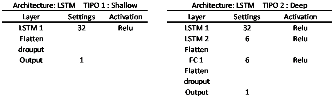
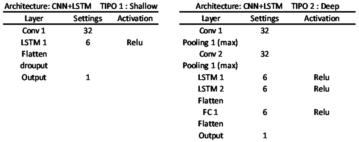
Appendix A. Model Architectures
Two models were created: one called shallow and another called deep, which has two additional intermediate layers. Table A1, Table A2, Table A3 and Table A4 show the internal structures of each of them.
Table A1.
DNN Model Architecture.
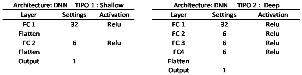 |
Table A2.
CNN Model Architecture.
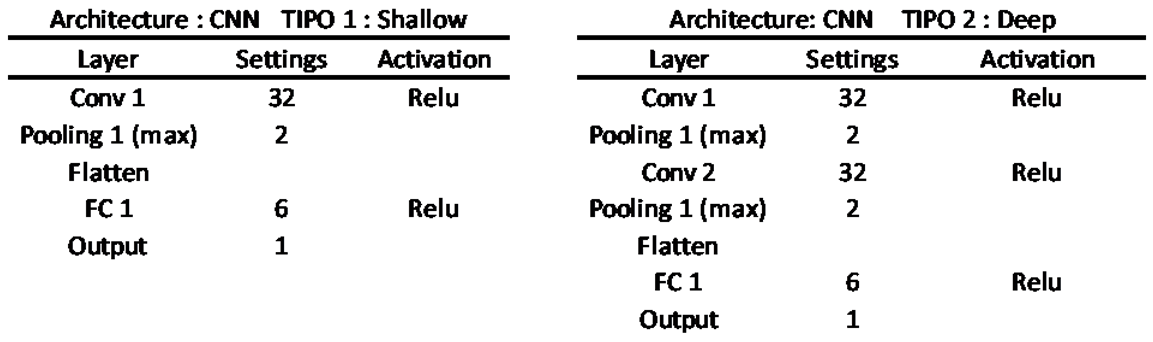 |
Table A3.
LSTM. Model Architecture.
 |
Appendix B. Hyperparameter Selection
Neural network models have internal parameters known as hyperparameters. Table B1 lists the main hyperparameters of the models. The last column contains the values obtained from the processes using the GridSearchCV function from Sklearn. These values were used in the experiments conducted in this study.
Table B1.
Hyperparameter Selection.
| Hyperparameter | Interval | Selection |
| Number of hidden layers | [1..100] | 1 to 6 |
| Number of neurons | [1..100] | 5 |
| Learning Rating | [0.0001..0.01] | 0,01 |
| Dropout rate | [0.1.. 0.5] | 0.1 |
| Activation function | Relu, Sigmoid, Tanh | Relu |
| Optimizer | Adam, RMSprop, SGD | Adam |
| Batch Size | [16..512] | 128 |
| Loss function | Mse, mae, mape | Mse |
| Kernel | [2..5] | 2 |
| Number of epochs | [10..500] | 30 |
Note: Table B1 were generated by the author
References
- Merce, R.A.; Grover-Silva, E.; Le Conte, J. Load and Demand Side Flexibility Forecasting. In Proceedings of the ENERGY The Tenth International Conference on Smart Grids, Green Communications and IT Energy-aware Technologies; 2020; pp. 1–6. https://minesparis-psl.hal.science/hal-03520220/.
- Khan, K.A.; Quamar, M.; Al-Qahtani, F.H.; Asif, M.; Alqahtani, M.; Khalid, M. Smart grid infrastructure and renewable energy deployment: A conceptual review of Saudi Arabia. Energy Strategy Reviews 2023, 50, 1012470. [Google Scholar] [CrossRef]
- Mystakidis; Koukaras, P.; Tsalikidis, N.; Iosnnidis, D. Compreeensive Review Of Techniques and Technologies. Energies 2024, 17, 1662. [Google Scholar] [CrossRef]
- Min, H.; Hong, S.; Song, J.; Son, B.; Noh, B.; Moon, J. SolarFlux Predictor: A Novel Deep Learning Approach for Photovoltaic Power Forecasting in South Korea. Electronics 2024, 13, 2071. [Google Scholar] [CrossRef]
- Mejía, M.; Villanueva, J.; Hernández, D.; Santos, F.; García, A. A Review of Low-Voltage Renewable Microgrids: Generation Forecasting and Demand-Side Management Strategies. Electronics 2021, 10, 2093. [Google Scholar] [CrossRef]
- Bunn, D.W. Short-term forecasting: a review of procedures in the electricity supply industry. J Opl Res Soc 1982, 33, 533–545. [Google Scholar] [CrossRef]
- Park, H.Y.; Lee, B.H.; Son, J.H.; et al. A comparison of neural network- based methods for load forecasting with selected input candidates. In Proceedings of the 2017 IEEE international conference on industrial technology (ICIT), Toronto, ON, Canada, 22–25 March 2017; IEEE: New York; pp. 1100–1105. [Google Scholar] [CrossRef]
- Peñaloza, A.K.A.; Balbinot, A.; Leborgne, R.C. Review of Deep Learning Application for Short-Term Household Load Forecasting. In Proceedings of the 2020 IEEE PES Transmission & Distribution Conference and Exhibition—Latin America (T&D LA), Montevideo, Uruguay, 28 September–2 October 2020; pp. 1–6. [Google Scholar] [CrossRef]
- Kong, W.; et al. Short-term residential load forecasting based on LSTM recurrent neural network. IEEE Transactions on Smart Grid 2017, 10, 841–851. [Google Scholar] [CrossRef]
- Mannini, R.; et al. Predictive Energy Management of a Building-Integrated Microgrid: A Case Study. Energies 2024, 17, 1355. [Google Scholar] [CrossRef]
- Elsworth, S.; Güttel, S. Time series forecasting using lstm networks: A symbolic approach. arXiv 2020, arXiv:2003.05672. [Google Scholar] [CrossRef]
- Glavan, M.; Gradišar, D.; Moscariello, S.; Juričić, D.; Vrančić, D. Demand-side improvement of short-term load forecasting using a proactive load management—A supermarket use case. Energy Buildings 2019, 186, 186–194. [Google Scholar] [CrossRef]
- Alom, M.Z.; Taha, T.M.; Yakopcic, C.; Westberg, S.; Sidike, P.; Nasrin, M.S.; Hasan, M.; Van Essen, B.C.; Awwal, A.A.S.; Asari, V.K. A state-of-the-art survey on deep learning theory and architectures. Electronics 2019, 8, 292. [Google Scholar] [CrossRef]
- Alzubaidi, L.; Zhang, J.; Humaidi, A.J.; Al-Dujaili, A.; Duan, Y.; Al-Shamma, O.; Santamaría, J.; Fadhel, M.A.; Al-Amidie, M.; Farhan, L. Review of deep learning: concepts, CNN architectures, challenges, applications, future directions. Journal of Big Data 2021, 8, 53. [Google Scholar] [CrossRef] [PubMed]
- Ungureanu, S.; Topa, V.; Cziker, A.C. Deep learning for short-term load forecasting—industrial consumer case study. Appl Sci 2021, 11, 10126. [Google Scholar] [CrossRef]
- Jiang, W. Deep learning based short-term load forecasting incorporating calendar and weather information. Internet Technology Letters 2022, 5, e383. [Google Scholar] [CrossRef]
- Son, N. Comparison of the Deep Learning Performance for Short-Term Power Load Forecasting. Sustainability 2021, 13, 12493. [Google Scholar] [CrossRef]
- Kuo, P.H.; Huang, C.J. A high precision artificial neural networks model for short-term energy load forecasting. Energies 2018, 11, 213. [Google Scholar] [CrossRef]
- Kim, T.Y.; Cho, S.B. Predicting residential energy consumption using CNN-LSTM neural. Energy 2019, 258, 114087. [Google Scholar] [CrossRef]
- Dudek, G. Multilayer perceptron for short-term load forecasting: From global to local approach. Neural Comput. Appl. 2020, 32, 3695–3707. [Google Scholar] [CrossRef]
- Amaral, L.S.; de Araújo, G.M.; de Moraes, R.A.R. Analysis of the factors that influence the performance of an energy demand forecasting model. Advanced Notes in Information Science 2022, 2, 92–102. [Google Scholar] [CrossRef]
- Amaral, L.S.; Araujo, G.M.; Moraes, R.A. An Expanded Study of the Application of Deep Learning Models in Energy Consumption Prediction. Springer, 2022. [Google Scholar] [CrossRef]
- Buildings. https://www.iea.org/energy-system/buildings.
- KawBamura, T. Distribution of discomfort index in Japan in summer season. J. Meteorol. Res. 1965, 17, 460–466. [Google Scholar]
- Ono, H.S.P.; Kawamura, T. Sensible climates in monsoon Asia. Int. J. Biometeorol. 1991, 35, 39–47. [Google Scholar] [CrossRef]
- JÚNIOR, A.J.; de Souza, S.R.; de Barros, Z.X.; Rall, R. Software para cálculo de desconforto térmico humano. Tekhne e Logos 2014, 5, 56–68. http://revista.fatecbt.edu.br/index.php/tl/article/view/280.
- Suganthi, L.; Samuel, A. Energy models for demand forecasting—A review. Renew Sustain Energy Rev 2012, 16, 1223–1240. [Google Scholar] [CrossRef]
- Curry, B.; Morgan, P.H. Model selection in neural networks: some difficulties. European Journal of Operational Research 2006, 170, 567–577. [Google Scholar] [CrossRef]
- Zhang, G.; Eddy Patuwo, B.; YHu, M. Forecasting with artificial neural networks: The state of the art. International Journal of Forecasting 1998, 14, 35–62. [Google Scholar] [CrossRef]
- Petropoulos, F.; Apiletti, D.; Assimakopoulos, V.; Babai, M.Z.; Barrow, D.K.; Taieb, S.B.; Bergmeir, C.; Bessa, R.J.; Bijak, J.; Boylan, J.E.; Browell, J. Forecasting: theory and practice. International Journal of Forecasting 2022, 38, 705–871. [Google Scholar] [CrossRef]
- Cogollo, M.R.; Velasquez, J.D. Methodological advances in artificial neural networks for time series forecasting. IEEE Lat Am Trans 2014, 12, 764–771. [Google Scholar] [CrossRef]
- Lippmann, R.P. An introduction to computing with neural adaptively trained neural network. IEEE Transactions onnets, IEEE ASSP Magazine, 4–22 April 1987.
- Sheela, K.G.; Deepa, S.N. Review on methods to fix number of hidden neurons in neural networks. Math. Problems Eng. 2013, 2013, 425740. [Google Scholar] [CrossRef]
- Chollet, f. (2015). Keras: The python deep learning API. Disponível em https://keras.io/.
- Ribeiro, A.M.N.C.; do Carmo, P.R.X.; Endo, P.T.; Rosati, P.; Lynn, T. Short- and Very Short-Term Firm-Level Load Forecasting for Warehouses: A Comparison of Machine Learning and Deep Learning Models. Energies 2022, 15, 750. [Google Scholar] [CrossRef]
- Gnanambal, S.; Thangaraj, M.; Meenatchi, V.; Gayathri, V. Classification algorithms with attribute selection: An evaluation study using WEKA. Int. J. Adv. Netw. Appl. 2018, 9, 3640–3644. https://www.proquest.com/openview/8f1f0774ec448384012948adb2af16e3/1?pq-origsite=gscholar&cbl=886380.
- Bendaoud, N.M.M.; Farah, N. Using deep learning for short-term load forecasting. Neural Comput. Appl. 2020, 32, 15029–15041. [Google Scholar] [CrossRef]
- Torres, J.; Martínez-Álvarez, F.; Troncoso, A. A deep LSTM network for the Spanish electricity consumption forecasting. Neural Comput. Appl. 2022, 1–13. [Google Scholar] [CrossRef] [PubMed]
Figure 1.
LSTM Model Structure. (Source: [18]).
Figure 1.
LSTM Model Structure. (Source: [18]).
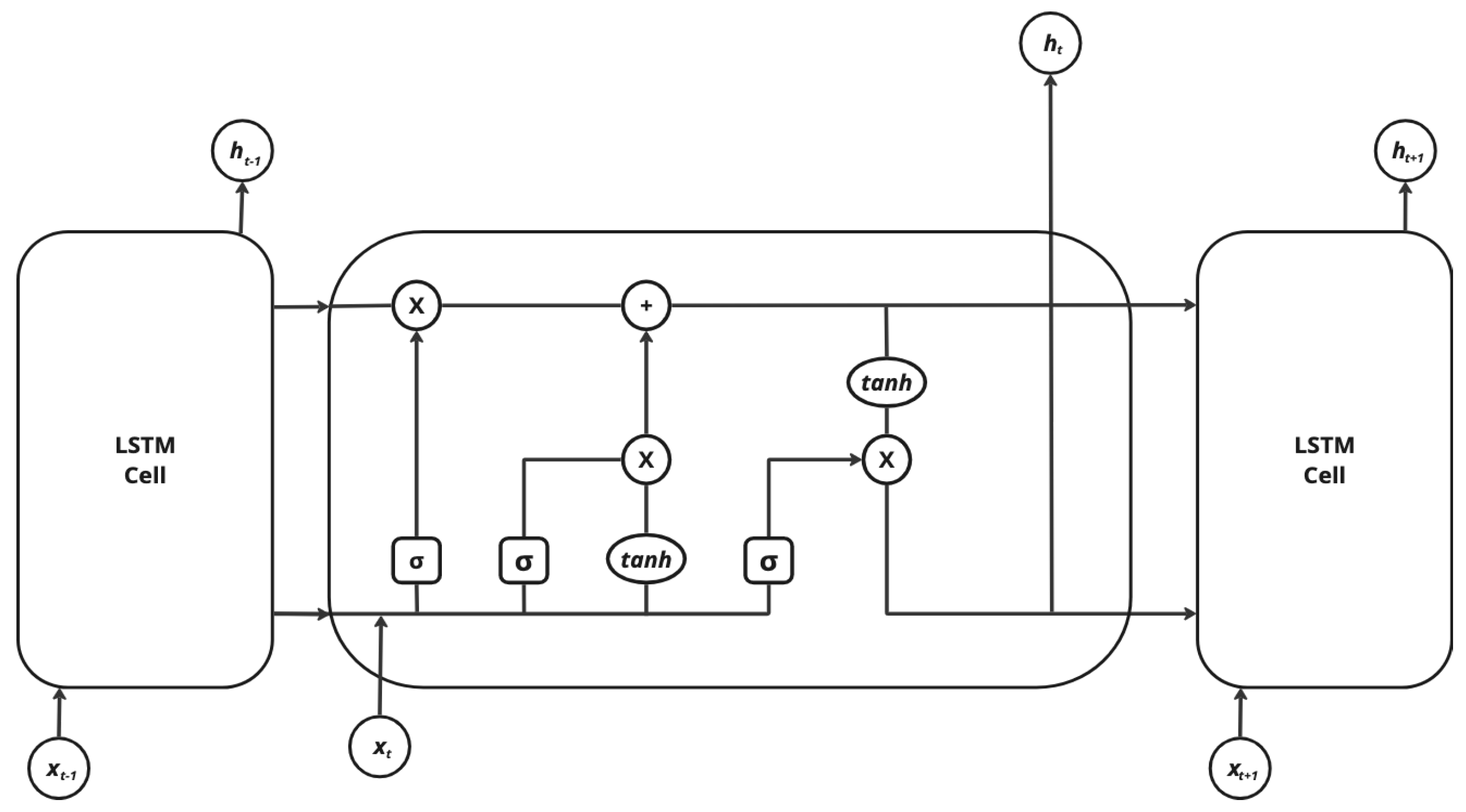
Figure 2.
CNN Model Structure. (Source: [17]).
Figure 2.
CNN Model Structure. (Source: [17]).
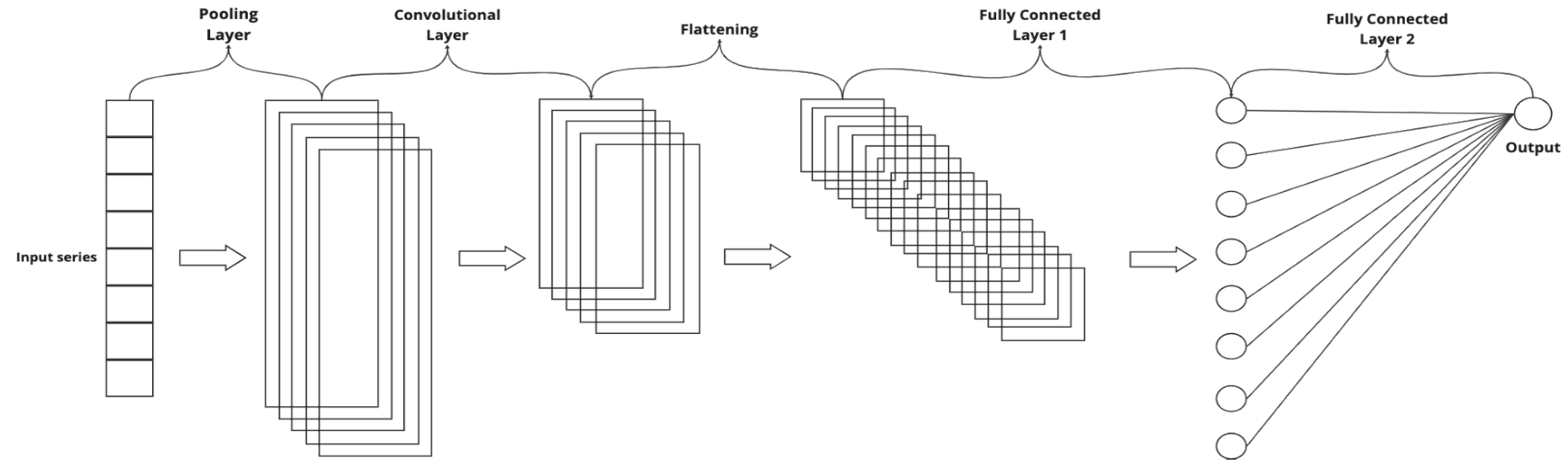
Figure 4.
Pipeline for creating an electricity consumption forecast models. (Source: Author).
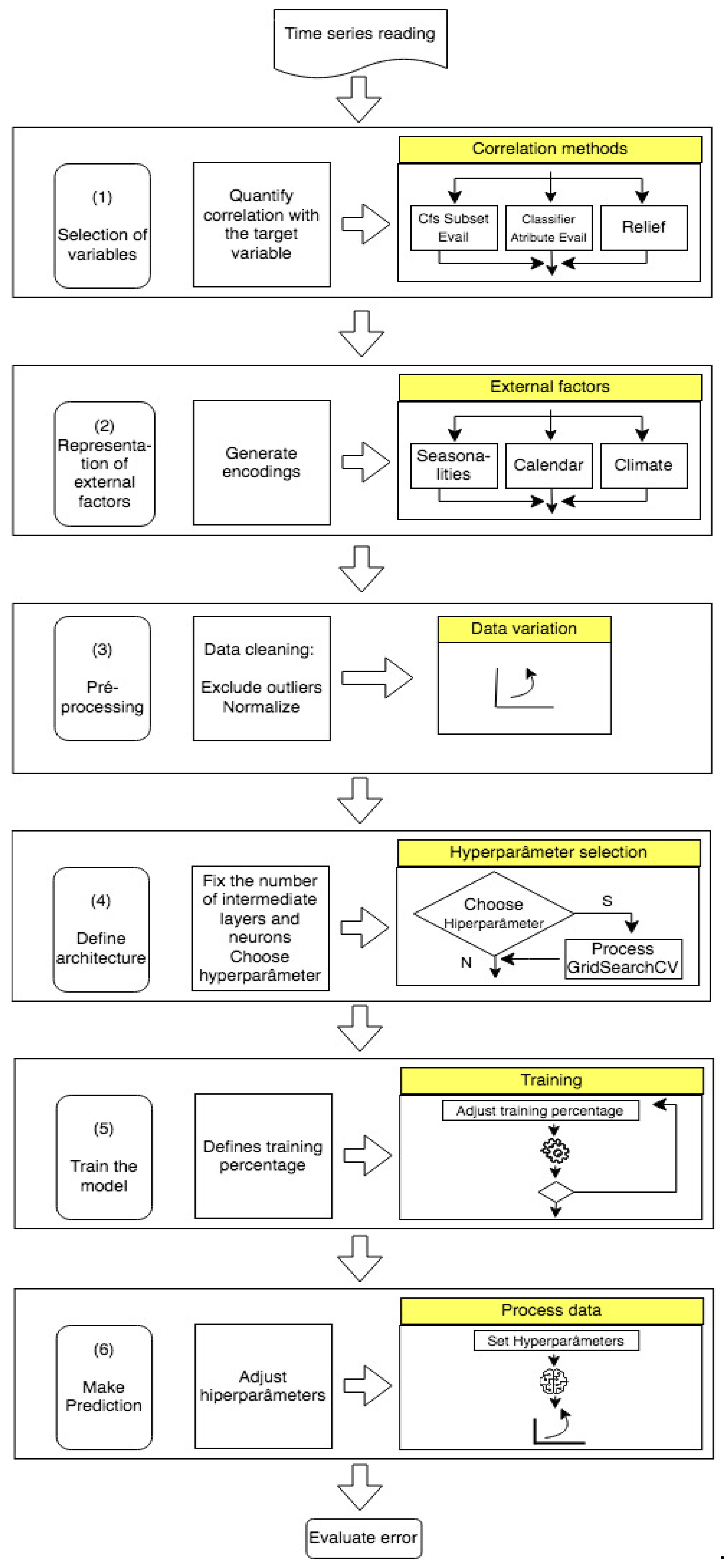
Table 1.
Relationships with Thermal Comfort Conditions.
| Interval | Condition |
|---|---|
| Id > 80 | Heat stress |
| 75 < Id < 80 | Unconfortable due to heat |
| 60 < Id < 75 | Confortable |
| 55 < Id < 60 | Uncomfortable due to cold |
| Id < 55 | Stress due to cold |
Table 2.
Date and Time of Day Encoding Methods.
| Name | Description | Value Range |
|---|---|---|
| Holiday | Holiday or not | [0,1] |
| Workday | Workday or not | [0,0.5,1] |
| Working | Working or not | [0,0.5,1] |
Source: [12].
Disclaimer/Publisher’s Note: The statements, opinions and data contained in all publications are solely those of the individual author(s) and contributor(s) and not of MDPI and/or the editor(s). MDPI and/or the editor(s) disclaim responsibility for any injury to people or property resulting from any ideas, methods, instructions or products referred to in the content. |
© 2024 by the authors. Licensee MDPI, Basel, Switzerland. This article is an open access article distributed under the terms and conditions of the Creative Commons Attribution (CC BY) license (http://creativecommons.org/licenses/by/4.0/).
Copyright: This open access article is published under a Creative Commons CC BY 4.0 license, which permit the free download, distribution, and reuse, provided that the author and preprint are cited in any reuse.


