Submitted:
18 June 2024
Posted:
18 June 2024
You are already at the latest version
Abstract
This study presents a comprehensive approach to trim optimization as a energy efficiency improvement measure, focusing on reducing fuel consumption for one RO-RO car carrier. Utilizing Computational Fluid Dynamics (CFD) software, the methodology incorporates Artificial Neural Networks (ANN) to develop a mathematical model for estimating key parameters such as brake power, daily fuel oil consumption (DFOC) and propeller speed. The complex ANN model is then integrated into a user-friendly software tool for practical engineering applications. The research outlines a seven-phase trim optimization process and discusses its potential extension to other types of ships, aiming to establish a universal methodology for CFD-based engineering analyses. Based on trim optimization results, the biggest DFOC goes up to 10.5% at 7.5m draft and up to 8% for higher drafts. Generally, in every considered case, it is recommended to sail with the trim towards the bow, meaning that the ship’s weight (ballast) should be adjusted to tilt slightly forward.
Keywords:
EEDI
; EEXI
; CII
; CFD
; ANN
; trim optimization
1. Introduction
With the aim to reduce emission of greenhouse gasses, in 2013 the International Maritime Organization (IMO) introduced the Energy Efficiency Design Index (EEDI) for new ships and later in 2023 the Energy Efficiency for Existing Ships Index (EEXI). These new measures initiated changes in the shipbuilding industry. By implementing these regulations, it is anticipated to reduce global CO2 emissions by 40% by year 2030 and 70% (or at least 50%) by year 2050, compared to the levels in 2008. All ships that fall under MARPOL Annex VI and have over 400 GT must meet the set criteria which is based on nominal ship data. IMO determined the parameters and procedure for calculating the required EEDI and EEXI, as well as the formula for calculating the attained EEDI/EEXI that must be lower than the required values. The required value for EEDI is determined by the formula:
where parameters a and c are based on the regression curve fit [1] of data from ships that were built between 1999 and 2009, and also depend on the type of ship. The required EEDI decreases over the years according to the formula:
where X is the specified reduction factor given in [2] through four phases. Values for EEXI are based on the required EEDI, taken into account with the adequate reduction factor from [3]. The requirements for EEXI are becoming slightly stricter with time, with the plan of EEXI and EEDI becoming equal in 2025. Beside the two mentioned energy efficiency parameters, IMO introduced operational efficiency indicators. In 2009 [4] the Energy Efficiency Operational Indicator (EEOI) was invented and is defined as the ratio of emitted CO2 per unit of transport work. EEOI never became mandatory but it is a representative value of the ship’s operational energy efficiency level for a consistent period of time. Another indicator came into force in 2023, the Carbon Intensity Index (CII), which is calculated as the ratio of the total mass of emitted CO2 to the total transport work undertaken in a specific calendar year, considering travelled distance, time spent underway and the amount of consumed fuel over a period of one year. As well as for EEDI and EEXI, attained [5] and required [6] values are also calculated for CII, where the attained CII has to be lower than the required, which decreases over time [7]. Based on the attained CII, the ship belongs to one of five energy efficiency categories (A, B, C, D, E). The boundaries between those categories and the calculation method for each ship type are defined in [8] and they depend on the ship’s DWT. Since CII is a mandatory parameter, all ships of 5000 GT or more are from 2019 obliged to record the relevant information (travelled distance, time spent underway and the amount of consumed fuel over a period of one year) under the Data Collection System (DCS) [9]. In case that a ship achieved class E for at least one year, or class D for three years in a row, it must create a plan for reducing CO2 emissions and satisfy the requirements for at least class C [10]. In 2013 IMO introduced the Ship Energy Efficiency Management Plan (SEEMP), which consists of three parts: ship management plan to improve energy efficiency, ship fuel oil consumption data collection plan and ship operational carbon intensity plan. Part I applies to all ships that fall under MARPOL Annex VI and have over 400 GT, while Part II and Part III apply for ships that have over 5000 GT and fall under MARPOL Annex VI.
Required EEDI = a(DWT)−c
Attained EEDI ≤ Required EEDI = (1 – X/100)·reference line value
Various measures can be considered in order to meet the energy efficiency requirements developed by the International Maritime Organization and attain reduction in CO2 emissions. Those measures are divided in two categories: operational methods and technical methods. Operational methods include: improvement in voyage execution [11,12], reduction of auxiliary power consumption [11,13], weather routing [10,12], “just in time” voyage [13], optimum ballast [10,12], optimum cargo distribution [12], energy saving utilities [14], optimum use of rudder and heading control systems [10], optimized hull and propeller maintenance [10], speed optimization [12,15], slow steaming [16,17] and trim optimization [12,18].
These measures can be applied for both existing ships as well as new ships. Technical measures are design related and therefore more favourable for new ships. These measures refer to wind-assisted propulsion, fuel type change [10,16,19], waste heat recovery [12], upgrading and maintenance of propulsion system, hull retrofit (bulb and/or stern modification, installation of energy saving devices [10], etc.
Optimum trim means that the angle of trim for a specific operating condition, regarding displacement and speed, provides minimum resistance which directly implies optimal efficiency level [12]. The resistance of the ship changes depending on the trim, although the displacement and speed stay the same [20]. Beneficial aspect of trim optimization is that neither hull modification nor engine upgrade is needed. The ship is trimmed if the draught at bow differs from the draught at the aft section of the ship. While negative trim indicates that the draught at the bow is greater than the draught at stern, positive trim implies the opposite. Every vessel is optimized for a number of conditions (even keel at full load and design speed, ballast condition, etc.), but the actual operating conditions usually differ from the expected ones [21]. It was confirmed in [22] that trim can affect the total resistance of a ship for various service speeds and the optimum trim for every speed is different. Trim optimization method is intended for minimizing the resistance in calm water and therefore minimizing fuel consumption which can be accomplished with a specially developed program for the ship. The results of [18] indicate the possibility of reducing total fuel consumption during a whole voyage by 1.2% by utilizing calculated optimum trim for whole voyage. 4250 TEU container ship sea trial with use of a trim optimizing program reported a main engine power reduction of 910 kW and energy saving rate of 9.2% [23]. Trim of the ship can be influenced by redistribution of ballast, fuel and/or load between tanks. Parameters that change when the ship is trimmed compared to even keel condition are wetted surface area, length of waterline and submerged hull form at bow as well as at stern [24]. Potential disadvantages of this method could be reduction of visibility, reduced freeboard, emergence of the propeller [25], underkeel clearance, seakeeping and shipped water on deck [26], and those should as well be taken into account while finding the optimum trim for an operating condition.
Calculating ship resistance in calm water by conducting model tests and numerical simulations provides data about resistance for different drafts and trims. As a result, a set of curves with highlighted lowest resistance for a specific draft is obtained, as in [22,27]. While onboard tools have this information at disposal, model tests are still being common and basins are equipped with traditional procedures and up-to-date insights to provide their proper execution, pursuing to measure small power variations within foreseen range of 0 to 4% of the total installed power [28], or 2% to 4% fuel consumption reduction [29]. With the advancement of technology and computers, CFD software calculations provide trim tables with an accuracy that can compete with the results gained from traditional model tests, with even less investments. Other methods that can be used to determine the optimum trim are sea trials and machine learning method. The shortcomings of these methods are that sea trials are fuel and time-consuming for determining the optimum ballast, while for obtaining information about the optimum trim with the machine learning method a lot of data from ship’s past voyages is needed [30]. In this study, the aim of work is focused only on applying CFD method on one RO-RO car carrier in order to optimize the trim for an energy efficient voyage and exploitation.
Application of CFD method for trim optimization for different ship types can be found in various existing studies. For example, in the research by [20] the effect of trim optimization for a container ship like MOERI (KCS) was a total resistance reduction of 2%, similar as the results of trim optimization for a US Navy ship [13]. A CFD investigation of the propulsion performance of a low-speed VLCC tanker at various initial trim angles was conducted by [31] and showed 1.76-2.12% total resistance reduction. [32] and [33] report even greater profit, such as fuel savings of up to 5% [32] and 6% reduction in delivered horse power [33]. Since the trim conditions can vary significantly, so do the results from trim optimization [34] highlights that in Series 60 the total resistance varies between the worst and best trims up to 11%. Trim optimization of bulk carrier in [35] results with total resistance reduction possibility by up to 14%. Savings for RO-RO ships were studied by [12] and indicated a possibility of up to 10.4% reduction in delivered power, or 1.2t fuel per day. Beside the calculation of optimal trim, specialized software that for input parameters quickly provide information about optimal trim have been mentioned [33,36].
Up to now, artificial neural networks (ANN) have found application in predicting fuel consumption, as demonstrated in studies by [37] and [38], which focused on utilizing NOON reports. Furthermore, ANN has been employed for forecasting ship speed, as evidenced by the work of [39]. Moreover, research efforts have extended to utilizing ANN for the joint prediction of ship speed and fuel consumption, leveraging data from sails, particularly in the case of a barquentine, as explored by [40]. The research [41] proposes a real-time hybrid electric ship energy efficiency optimization model considering time-varying environmental factors, aiming to optimize the EEOI under wind and wave conditions while maintaining speed limits, resulting in an average reduction of fuel consumption by 13.4% and real-time EEOI by 15.2%. In [42] is presented a real-time prediction model of ship fuel consumption through BP neural network training-related data, and further used it for ship speed optimization.
In today’s complex technological landscape, the integration of various disciplines is becoming increasingly vital for tackling engineering challenges. By bridging the fields of naval engineering, CFD, ANN and practical application development, this study not only underscores the importance of multidisciplinary association but also showcases its benefits in addressing real-world problems within the maritime industry. Through the synergy of these varied fields, novel solutions can be developed to optimize ship operations or design, enhance fluid flow analysis accuracy, and streamline decision-making processes. Moreover, the utilization of ANN enables the creation of sophisticated mathematical models that can effectively capture complex relationships and patterns within maritime systems, paving the way for more precise simulations and predictive analytics. Furthermore, the development of user-friendly applications facilitates the seamless implementation of these advanced methodologies, empowering stakeholders to leverage cutting-edge insights for improved vessel performance and operational efficiency. Essentially, this methodology not only promotes scientific comprehension but also encourages innovation and pragmatic breakthroughs in the field of maritime engineering, thus helping in a long-term growth of maritime technologies.
2. Methods
The conducted work consists of several phases: 1) 3D modeling; 2) First level verification of the reliability of the digital twin (3D model); 3) Open Water Test (OWT); 4) Second level verification of the reliability of the 3D model; 5) Trim optimization; 6) Determination of a mathematical model for assessing optimal trim, ship speed, engine (brake) power, daily fuel consumption, and propeller speed; 7) Programming an application based on previously conducted analyses. In this study various software have been used: StarCCM+ for CFD analysis, aNETka for mathematical model determining and MATLAB for application development.
In Table 1 are given ship’s (RO-RO car carrier) principal particulars.
Propeller geometry characteristics are presented in Table 2.
2.1. 3D Modeling
3D modeling is the first necessary step before conducting CFD simulations. Creating a 3D representation of the RO-RO vessel involved using existing documentation: hull construction drawings, rudder construction drawing and propeller drawing. This digital twin includes detailed modeling of the hull, rudder, and propeller, with the goal of faithfully capturing the ship’s attributes and performance.
2.2. First Level Verification
First level verification involves comparing hydrostatic data such as displacement (Δ), block coefficient (CB), Longitudinal center of buoyancy (LCB), and wetted surface (WS) of the 3D model with data given in the Trim & Stability booklet for various drafts. No parameter should deviate more than 1% from (as per authors experience 1% deviation enables enough accuracy) its corresponding value given in the Stability Booklet.
2.3. Open Water Test
The OWT is a method for determining propeller characteristics such as thrust coefficient, torque coefficient, and propeller efficiency. The procedure for determining these coefficients through model tests is defined in [43]. In this case, model testing was not conducted; instead, propeller parameters were determined through CFD simulation, following the procedure described in [44]. According to this document, CFD results of the OWT are considered valid if they do not differ more than 3% from results obtained by model testing within the relevant propeller operating range. It is also emphasized that if model test results of the propeller are not known, an additional OWT with the appropriate B-series propeller model should be conducted. An appropriate B-series propeller is considered one with the same geometric characteristics (diameter, pitch, ratio of characteristic areas) as the original propeller installed on the considered ship. The 3D model of the B-series propeller was obtained using the B-series Propeller Generator available online [45]. OWT results of the B-series propeller should not deviate more than 3% from results obtained with mathematical model for the same geometric parameters. If this condition is met, the same CFD calculation methodology is applied to the original propeller, and results obtained this way are considered valid. A mathematical model can be found in [46].
The simulations are conducted using a steady state numerical flow model, solved in the rotating frame of reference. The numerical method used is called Multiple Reference Frames (MRF), where in one part of the domain the equations are solved in rotating frame of reference, while in the rest of the domain stationary frame of reference is used.
Figure 1 shows the domain of the open water test CFD setup. The outer cylinder shows the far-field boundary of the domain, while the inner, smaller cylinder represents the boundary between the rotational frame of reference and stationary frame of reference. Diameter and length of small cylinder are 4D, while diameter and length of large cylinder are 10D. The propeller is positioned downstream from the shaft. All simulations are conducted in full scale.
The same grid refinement options were used for both propellers grids (B series propeller and Original propeller) are presented in Figure 2.
Turbulence modelling is performed using the k-ω SST model. Inflow turbulence intensity was set to 1% relative to the inflow speed. The inflow speed conditions, and rotation rate of the propeller are selected to closely resemble the conditions expected at self-propulsion conditions.
2.4. Second Level Verification
Second level verification involves conducting CFD simulation for a draft for which there are available results from model tests or sea trials. The difference between results obtained by CFD analysis and model tests/sea trials should not be greater than 5%.
The equations are discretized using collocated Volume of Fluid (VOF) multiphase method implemented within software. It is used for large–scale two–phase (in this case sea water (ρw=1.025 t/m3) and air (ρA =1.212 kg/m3) at 18⁰C) flows encountered in naval hydrodynamics. A two–phase, incompressible, turbulent and viscous flow model is employed, governed by the continuity and Navier-Stokes equations:
where V stands for the velocity vector field, p is the pressure, Tv is the viscous stress tensor and fb is the resultant of the body forces.
The VOF multiphase Eulerian approach model implementation in Simcenter STAR-CCM+ belongs to the family of interface-capturing methods that predict the distribution and the movement of the interface of immiscible phases. This modeling approach assumes that the mesh resolution is sufficient to resolve the position and the shape of the interface between the phases.
An important quality of a system of immiscible phases (air and water) is that the fluids always remain separated by a sharp interface. The High-Resolution Interface Capturing (HRIC) scheme is used to mimic the convective transport of immiscible fluid components, resulting in a scheme that is suited for tracking sharp interfaces.
2.4.1. Actuator Disc Propeller Model
The body force propeller method is used to model the effects of a propeller such as thrust and thereby creating propulsion without actually resolving the geometry of the propeller. The method employs a uniform volume force distribution over the cylindrical virtual disk. The volume force varies in radial direction, so the total force can be calculated as volume integral for the whole modeled cylinder. The radial distribution of the force components follows the Goldstein optimum [47] and is given by:
where r* is the normalized disc radius defined as:
where r’=r/Rp and rh’=Rh/Rp. Volume force fbx is body force component in axial direction, r is the radial coordinate, Rh is the hub radius and Rp is the propeller tip radius. Coefficient Ax is defined as:
where T stands for propeller thrust and td is the virtual disk thickness. More about this can be found at [48]. The simulation is performed for a certain operating point specified by thrust (T). The advance ratio is calculated by solving the following equation numerically (J—advance coefficient, D—propeller diameter):
where KT is evaluated from the propeller performance curve and KT’ is evaluated as:
With KT available, the thrust is calculated for the propeller:
With T (T(Operating point)) available, the axial body force component can be calculated. Inflow plane is the plane inside actuator disk where volume-averaged velocity and density are computed. Input thrust in this part of the simulation is equal to the total resistance that is evaluated as sum of the pressure resistance and viscous resistance of the hull with rudder included.
The wake fraction (w) is extracted at propeller axis plane in steady resistance simulation.
Thrust deduction factor is calculated as per:
where RT is total resistance of the ship evaluated in steady resistance simulation.
2.4.2. Steady Resistance Simulations
Total resistance, including viscous and pressure resistance, is obtained by re-running the self-propulsion simulation with disabled actuator disc. This procedure implies the same mesh as it was used earlier but only without an actuator disc.
2.4.3. Boundary Conditions
Fluid domain dimensions are defined as follows (from origin) this:
- Inlet: 2.5 Lpp;
- Outlet: 3 Lpp;
- Bottom: 1.5 Lpp
- Top: 1 Lpp;
- Port Side: 2 Lpp;
- Starboard Side: 2 Lpp.
2.4.4. Rigid Body Motion
Two degrees of freedom are allowed for the motion for the vessel, namely pitch and heave, allowing for dynamic trim and sinkage of the vessel.
2.4.5. Mesh
The triangle surface meshing method has been used to build the mesh. Prism layer mesher generates prismatic cell layers next to the boundary layer. The number of these layers is calculated as per:
where sf=1.3 is stretch factor, δ is boundary layer thickness and y1 is the first layer thickness. These cells help to captur0e the viscous effects in boundary layer correctly in the region which thickness is calculated as per [49]:
where Lwl is length at waterline of the ship and Re is Reynolds number (Lwl in subscription means that Reynolds number is calculated with waterline length as a reference value, otherwise Lpp is used). Trimmed cell mesher creates a volume mesh by cutting a template mesh with the surface geometry. First layer thickness is calculated for y+ = 150 by following guidelines [44] where it is emphasized that y+ should be in a range from 30 to 300. This value (150) is used as target factor to be ensured that the actual y+ values will fall within the required range.
where υ is kinematic viscosity and uτ is shear velocity. Shear velocity or frictional velocity is fictious quantity and it characterizes the shear at the boundary layer and it is given by:
where τw is wall shear stress. This presents a contradiction: determining the thickness of the initial layer requires knowing the stress on the vessel’s hull, which in turn needs to be assessed using CFD. Hence, the recommendation from ITTC [43,50] is utilized in this scenario to compute the wall shear stress for the hull.
where k is a form factor, CFS is frictional resistance coefficient and CA is the correlation allowance.
Form factor is calculated as mean value of the equations obtained by Grigson, Wright, and Conn and Ferguson given in [51]:
A grid convergence study is performed to assess the convergence of the results by systematically refining a specific input parameter in StarCCM+. In this study, three simulations are conducted, where the chosen input parameter is varied while keeping all other parameters constant. The refinement value used in this study aligns with the guidelines specified in [52] and is set to be uniform (. By systematically refining the input parameter and comparing the results from the different simulations, the grid convergence study aims to determine the level of convergence and establish the appropriate grid resolution for accurate and reliable results.
Convergence ratio is defined as:
where is the difference between solution obtained using medium and fine mesh and is the difference between solution obtained using coarse and medium mesh. R is used for estimation of convergence conditions: monotonic convergence is achieved when 0<R<1, oscillatory convergence is achieved when -1<R<0 and divergence is achieved when |R|>1. Numerical uncertainty and error for monotonic convergence condition is estimated using generalized Richardson extrapolation (RE). The order of accuracy is calculated as per:
The generalized RE solution () can be derived by:
To estimate the grid uncertainty UG, a safety factor approach is employed, defining UG as:
where FS=1.25 is a safety factor. The normalized uncertainties are calculated as follows:
2.4.6. Post Processing
In the numerical simulations conducted for this study, the direct consideration of roughness effects and air resistance resulting from the presence of a superstructure is not included. However, these effects are accounted for in the post-processing stage by following the recommended procedures and guidelines outlined in [53]. The ITTC guidelines provide specific methodologies for incorporating the effects of roughness and air resistance into the analysis, allowing for an assessment of the overall performance and characteristics of the ship. Roughness allowance (∆CF) is calculated as per [54]:
and air resistance coefficient () [50] is:
where ks indicates the roughness of hull surface equals to 150 ∙10-6 m [54], and AVS is the projected area of the ship superstructure to the transverse plane. New total resistance is calculated as:
where CT refers to total resistance coefficient obtained as a result from CFD simulation.
New thrust is calculated as per:
Together with propeller performance data (KT, KQ, η0(J)), new operating point is obtained by numerical solving of equation:
Once the advance ratio coefficient is obtained, the propeller speed (n) and torque (Q0) can be evaluated:
where KQ is evaluated from the propeller performance curve and Q0 is torque in open water condition. Hence actuator disk approach has been used in this case, relative rotative efficiency is adopted to be 1, that means that torque is calculated as:
Finally, brake power can be evaluated as:
where ηS is shaft efficiency, adopted to be 0.99. Hull efficiency is considered to be the same as in steady resistance simulations i.e., w’=w and t’=t, where w’ and t’ are wake fraction coefficient and thrust deduction factor in post processing.
Calibration factors Cn and CPb are calculated as the average ration between model test (MT) results and CFD results for propeller speed (n) and brake power (Pb).
2.5. Trim Optimization
Trim optimization was conducted for drafts of 7.5m, 8m, and 8.7m at speeds of 12.5kn, 15kn, and 18kn at 7 different conditions (trims). The range of trims goes from -1.5m to 1.5m with a 0.5m step. Negative sign means trim by bow and positive sign, trim by stern. The outcome of trim optimization in CFD analysis typically involves determining the optimal trim settings for a vessel at considered drafts and speeds. This optimization aims to minimize resistance and ensure optimal performance under different operating conditions. By adjusting the vessel’s trim, operators can achieve better hydrodynamic characteristics, leading to improved overall performance and operational efficiency. With available specific fuel oil consumption (SFOC) curve as a function of Pb, a possible reduction of fuel consumption was also calculated.
2.6. Mathematical Model for Assessing the Outcomes from Trim Optimization
First outcomes from CFD simulations are brake power and propeller speed for one ship speed and draft i.e., trim i.e., displacement. The results are presented in the form of relative differences between the brake power of the trimmed ship and the ship on an even keel. A negative sign indicates that there is a saving, i.e., a reduction in the required brake power for that case. A graphical example of the results is shown in Figure 3a, where the relative brake power savings are depicted as an area with ship speed on the x-axis, trim on the y-axis, and relative power savings on the z-axis. The optimal (favorable) sailing zone is depicted in green on the same diagram, meaning that at current trim and speed, less power is required compared to when the ship is sailing on an even keel. The yellow zone represents the transitional zone where the change in required brake power is negligible, while the red zone is the zone to be avoided because more power is needed for the ship to sail at the same speed compared to sailing on an even keel. Each point on the surface in Figure 3 a corresponds to a certain displacement, where it depends solely on the trim. For easier calculation, a surface Δ(trim, Vs) is formed from each line Δ(trim), and surfaces for all three considered drafts are shown in Figure 3b. In order to have smooth surfaces, all values between estimated from CFD analysis are linearly interpolated. Therefore, initial matrix 3x7 (3 speeds, 7 trims) is reshaped to 151x111 with a speed step 0.05kn and trim step 0.02m.
Additionally, values between drafts of 7.5m to 8m and from 8m to 8.7m are linearly interpolated with a step of 0.01m. Thus, from the initial matrix of 3x7x3 (3 speeds, 7 trims, 3 drafts), matrices (Σm) of size 151x111x120 are obtained where m is Δpb or Δ.
The daily fuel oil consumption (DFOC) is estimated based on the determined brake power from CFD simulation and the available specific fuel oil consumption (SFOC) curve for the engine installed on the ship. The SFOC curve is approximated by a sixth-degree polynomial:
The mentioned polynomial provides SFOC values with an average error of 0.02% compared to the exact available values from reference document.
With evaluated DFOC for each brake power, the same diagrams as they are shown in Figure 4 can be created (Figure 5).
In operations, after loading cargo onto the ship, only the displacement is known. The goal of the conducted trim optimization is to find the optimal position, i.e., trim, and recommend the sailing speed based on that single parameter. The optimal trim and recommended speed are those at which the greatest savings in brake power, and consequently fuel consumption, are achieved. The mathematical expression of the above statement is as follows:
where is the biggest brake power reduction where the corresponding displacement is within a tolerance (=0.0001) of the target displacement (). Index i represents speed, j represents trim and k represents brake power reduction i.e., displacement in matrix Σm. When is found, it is easy to extract indices i, j and k and therefore to derive optimum trim and speed for corresponded displacement i.e., mean draft. In practice, there may be a need for speed as an input parameter, which depends on operational requirements, and this case will be addressed in subsequent work.
2.6.1. Mathematical Model for Assessing Brake Power, DFOC and Propeller Speed
A sophisticated mathematical model utilizing Artificial Neural Networks (ANNs) has been developed based on CFD results. By specifically addressing the challenges posed by non-simulated loading conditions, this model offers a solution for estimating parameters such as brake power, propeller speed, and DFOC.
At its core, the model employs a feedforward artificial neural network (FFANN), a fundamental architecture in machine learning and deep learning. The FFANN’s structure comprises interconnected layers of neurons, including an input layer, one or more hidden layers, and an output layer (Figure 6). Each neuron is equipped with adjustable parameters called biases, which introduce flexibility by allowing for offsets or shifts in output. During training, these biases are fine-tuned to better fit the data and ensure accurate estimation of the desired parameters.
One of the key features of the FFANN is its one-directional flow of information, from the input layer through the hidden layers to the output layer. This design simplifies the learning process and enables efficient modeling of complex data relationships. Additionally, activation functions embedded within neurons introduce non-linearity, enabling the network to capture patterns present in real-world data.
Overall, this innovative approach represents a significant step forward in the advancement of engineering solutions. It not only addresses the inherent challenges of non-simulated loading conditions but also sets a precedent for the application of artificial intelligence in optimizing the performance of complex systems. As further research and development are conducted in this field, the potential for ANNs to revolutionize engineering practices and transportation systems continues to expand.
In the context of a feedforward artificial neural network (FFANN), the connections between neurons are governed by weights, which dictate the strength of the connections. These weights are adjusted during the training process using an algorithm called backpropagation. The name “backpropagation” stems from its mechanism of iteratively propagating errors backward through the network to adjust the weights and biases of neurons.
The training process ©nvolves two phases: the forward pass and the backward pass. During the forward pass, input data is fed into the network, and predictions are made based on the current weights and biases. These predictions are compared to the actual outputs, and the resulting error is calculated.
In the backward pass, this error is propagated backward through the network, layer by layer. The gradient of the error with respect to each weight and bias is computed using techniques like the chain rule of calculus. These gradients indicate the direction and magnitude of adjustment required to minimize the error. The weights and biases are then updated accordingly.
At each neuron, the weighted sum of inputs is computed by multiplying each input value by its corresponding weight and summing the results. This sum is then combined with the neuron’s bias:
where —activation function, —output signal, of th neuron in th layer, output of th neuron in th layer, —weights connected to neuron and corresponding bias.
The resulting value is passed through an activation function, which introduces non-linearity into the network. Common activation functions include sigmoid, tanh and others, each serving different purposes in facilitating learning and modeling complex data relationships. In this case, sigmoid function is used:
The general form of the function is:
where:
- Xk—Input parameters (number of neurons in input layer);
- Yu—Output parameters (number of neurons in output layer);
- f1,f2,…,f(p-1),fp—activation function;
- k,j,©,…,v,w—number of neurons in each layer;
- A,B,…,P—weights between layers;
- a,b,…,p—weights between neurons in each layer and bias.
The software that has been used for training the ANN in this study is called aNETka [55] developed in LabVIEW. The output file from this software is not direct mathematical model, just weights coefficients and four additional parameters called Down offset Input (DIk), Down offset Target (DTu), Up offset Input (UIk) and Up offset Target (UTu).
The rest of parameters are calculated as follows:
In the trim optimization study, data obtained from CFD analysis, including brake power, DFOC, and propeller speed, were utilized as inputs for training an Artificial Neural Network (ANN). This ANN establishes correlations between draft, speed, trim, displacement, and the aforementioned performance parameters.
The applicability range of the model is defined within specific boundaries for each parameter: draft (Ts) ranges from 7.5 to 8.7 m, speed (Vs) ranges from 12.5 to 18 kn, trim ranges from -1.5 to +1.5 m and displacement (Δ) ranges from 18079 to 22884m3. The input dataset for training consists of a 63x7 matrix, where number 63 represents the total number of CFD simulations conducted and number 7 denotes to each parameter. Four parameters are designated as the input layer (draft, displacement, trim, speed), while the remaining three represent the output layer (propeller speed, brake power, DFOC).
Prior to training, all data were normalized within the range of 0.05 to 0.95 to ensure the stability of activation functions, which can be sensitive to extremely small or large input values. This normalization step enhances the convergence and effectiveness of the training process.
For testing purposes, 8% of the total input parameters (5 out of 63) were reserved, while the remaining data was allocated for training. The training process was programmed to iteratively adjust the weights and biases of the network, stopping when the Root Mean Square (RMS) percentage error reached the target threshold of 1%:
where TV—target values, OV—ANN output values, —number of values
When creating a neural network model, it’s vital to carefully consider the number of neurons in each layer and the presence of hidden layers. These decisions must be well-informed and tailored to match the complexity of the problem at hand and the specific attributes of the dataset.
2.7. Trim optimization software application
Formulas derived for a particular purpose may not always be user-friendly, leading to the creation of an application to facilitate their use. In this case, an application developed using MATLAB’s App Designer package offers a user-friendly interface for utilizing these formulas. The application allows users to input only one parameter i.e., displacement and obtain corresponding output values efficiently: optimum trim, speed, propeller speed, brake power and DFOC. This enables users to quickly obtain results without the need for manual calculations.
3. Results
The results in this section will be presented by subsections in the same order, i.e., following the phases outlined in the section 2 (Methods).
3.1. 3D Modeling
In Figure 7, a 3D model and characteristics sections of waterlines (a), buttocks (b) and frames (c) are depicted in various projections obtained based on construction drawings.
The propeller underwent a modeling process, aligning with the specifications outlined in the reference drawing. A comparison was conducted between the 3D model of the propeller and the reference drawing to ensure precise adherence to the intended design. The findings of this comparison are visually presented in Figure 8, offering a clear representation of the propeller’s details and shape. The 3D model of the propeller (Figure 9a) enables engineers and designers to perform CFD simulations and evaluate performance characteristics. The rudder was modeled to faithfully represent its original design but without any gaps between rudder shaft and rudder shell (Figure 9b).
3.2. First Level Verification
The reliability of the developed 3D model was assessed by comparing its calculated hydrostatic parameters against the corresponding ones given in the Trim & Stability booklet. The corresponding percentage deviations between CB, V, LCB and WS are listed in Table 3.
It can be easily observed that deviations between calculated and reference values of hydrostatic data are less than 1% especially for the range of interest (drafts 7.5m, 8.0m and 8.7m).
3.3. Open Water Test
Graphical representation of CFD results (KT, KQ, η0) from conducted OWT with B-series propeller with data obtained with mathematical model is presented in Figure 10a, while relative differences between each evaluated parameter is presented in Table 4.
As the results for each of the advance coefficients are within the prescribed 3%, the CFD calculation methodology is considered valid, therefore, with the same setup, original propeller OWT was conducted and results are presented in Figure 10b.
3.4. Second Level Verification
Obtained results from CFD OWT simulation with original propeller are used as an input propeller characteristics data in self-propulsion simulations. First group of simulations were conducted at design draft (7.8m) and speeds of 17kn, 19kn and 21kn because for these draft and speeds model test data are available.
In the Figure 11 meshed domain is shown. For better evaluation of free surface, additional refinement zones are defined in wave field zones and near the hull (Figure 12a,b).
Results from completed self-propulsion simulations and steady resistance simulations by following procedure described in section 2.4 are presented in Table 5 where Rp is pressure resistance and Rv is viscous resistance.
Results from CFD analysis and model test data are graphically presented in Figure 13. In Figure 13a brake power as a function of ship speed curve is depicted while in Figure 13b brake power as a function of propeller speed is presented.
Calibration factors are Cn=1.05 and CPb=1.04 which means that 5% deviation requirement in results compared to model test is met.
In the Figure 14 are presented y+ values for the underwater part of the hull and average y+ value is pointed out (average y+ = 70.61). Particular case is extracted from steady resistance simulation at speed of 18kn at 7.5m draft. For all other speeds y+ values do not deviate from aforementioned.
Three different meshes were considered for the grid uncertainty study with mesh sizes of 1.852 million cells (coarse), 3.628 million cells (medium), and 7.454 million cells (fine). The study was conducted at a speed of 18 knots at 7.5m draft (even keel). The results of the study, including the grid uncertainties for thrust are presented in Table 6.
3.5. Trim Optimization
Trim optimization CFD study was performed at 7.5m, 8m and 8.7m draft for a range of speeds 12.5kn, 15kn and 18kn at 7 different loading (trim) conditions and coarse mesh. Therefore, results for obtained propeller speed, brake power and estimated DFOC are presented in Table 7, Table 8 and Table 9, respectively.
3.6. Mathematical Model for Assessing the Outcomes from Trim Optimization
Brake power reduction and DFOC reduction are linearly interpolated for additional trims and speeds (values between considered in CFD analysis) and results are graphically presented for three considered drafts in Figure 15 and Figure 16. Optimum trim and speed are also depicted with red points in Figure 16. Black line in Figure 15 and Figure 16 represents neutral line, i.e., the state of even keel against which brake power savings and DFOC savings are calculated.
The biggest reduction in DFOC can be achieved at 1.5m trim by bow, 7.5m draft and speed of 15.17kn (10.5%), while for the 8m and 8.7m draft, the biggest reduction in brake power is at 12.5kn (8%, 7%, respectively). Sailing at 12.5kn instead of 15kn or 18kn, and maintaining an even keel, can result in greater fuel savings for higher drafts. Although greater fuel savings might be achievable with a greater trim by bow, but any condition more than -1.5m trim by bow cannot be attained on the current ship.
In Figure 17, wave fields are depicted for the case of Vs=15kn, Ts=7.5m at trim=0m (Figure 17a) and at trim=-1.5m (Figure 17b). It is evident that the total wave amplitude when trimmed towards the bow by 1.5m is reduced by 0.25m, indicating a decrease in pressure resistance—displacement ratio for 15% (see Table 10).
In the Figure 18 are presented free surfaces in center line and along the hull at two different conditions: trim = 0m (white hull) and trim = -1.5m (yellow hull). Black line corresponds to free surface level at zero trim condition while red line corresponds to free surface level at trim by bow for 1.5m. In the Figure 18a are presented bow waves, while in the Figure 18b are presented stern waves. Peak-to-peak amplitude of the bow wave is reduced by 0.64m while the stern wave is reduced for nearly 1m when the ship is trimmed towards the bow by 1.5m.
For others drafts and trims, the impact of bow trim remains similar, nevertheless a less noticeable reduction in pressure resistance. It seems that this kind of the bulb has better effect when it is more submerged into the water at lower drafts. This contradicts what is highlighted in numerous literature sources, including [56] and [57] but it is not the first time that the same conclusion with fully submerged bulb has been set [58,59].
3.6.1. Mathematical Model for Assessing Brake Power, DFOC and Propeller Speed
Unfortunately, a single mathematical model did not attain the desired RMS within a reasonable training timeframe and iteration count. As a result, two separate mathematical models were devised: one focusing on brake power and DFOC and the other dedicated to propeller speed prediction. The formula for brake power follows a general form:
The general form of the function for DFOC is:
The general form of the function for propeller speed is:
Configurations of neurons for both mathematical models are presented in the Figure 19a,b.
Obtained coefficients for Equations (51) and (52) are given in Table 11, Table 12, Table 13, Table 14 and Table 15, while coefficients for Equation (53) are given in Table 16, Table 17, Table 18 and Table 19.
The standard deviations of the relative differences in brake power, DFOC, and propeller speed calculated values using Equations (51)–(53), and the results obtained from the CFD analysis for the same three parameters are 0.6%, 0.6%, and 0.2%, respectively.
3.7. Trim Optimization Software Application
Development of software focusing on trim optimization is another step forward that demonstrates how engineering and technical practice can be more effectively connected. The equations obtained (51), (52), and (53) are very complex and not suitable for manual calculation. Additionally, the matrix obtained through interpolation of the CFD analysis results contains over 2 million elements (a 151x111x120 matrix), making tabular or graphical representation of the results will be impractical for the average user. Therefore, the most elegant solution is to develop an application with a graphical interface. Today, there are many software tools that operate based on writing in various programming languages, but this task is addressed to other engineering disciplines. This paper demonstrates the development of a software tool within MATLAB App Designer. MATLAB App Designer is highly suitable for rapid development of simple applications as it has certain functions predefined within the Component Library. In this specific case, only three predefined functions were used: “Button,” “Edit Field,” and “Label.” The interface design is depicted in Figure 20:
In the “Input displacement” label user should insert current displacement in cubic meters in the range from 18078 to 22884m3. The estimation of the optimal trim, corresponding mean draft, estimated speed, brake power, DFOC, and propeller speed is performed by simply clicking the “Calculate” button. In case the user inputs a displacement below or above the specified values despite the stated applicability limits of the mathematical model and initiates the calculation, a message will appear on the screen: “Displacement is out of range” (see Figure 21).
If a displacement within the specified limits is entered, and the “Calculate” button is clicked, all the data is instantly displayed (see Figure 22).
The application provides results based on previously obtained mathematical models for estimating the optimal trim, speed, corresponding mean draft, brake power, DFOC, and propeller speed. There is also a note that sign “-“ in Optimum Trim label corresponds to trim by bow. Due to the specified project task, which required trim optimization at certain speeds, trims, and drafts rather than displacements, it is clear that for the same draft and different trims, the vessel has different displacements. Considering the upper limit of the performed calculations with a draft of 8.7m and taking into account various trims, accordingly, the upper limit of displacements for which the calculations were performed at this draft (8.7m) is variable (refer to Figure 4b). Considering the obtained results, there is a displacement range where the optimal trim is 0m, meaning that sailing on an even keel is recommended (see Figure 23). This zone starts from the displacement corresponding to a draft of 8.7m and even keel position.
The mathematical model does not take draft as an input parameter but determines the mean draft by seeking the optimal trim for a given displacement. It’s logical to apply the recommendation of optimal trim obtained from the mathematical model only through additional ballasting of the vessel if achieving the optimal trim cannot be attained with the existing ballast water in the tanks (if any). This is manifested by further increasing the displacement. Therefore, it’s necessary to rerun the application with the new displacement. Through a few iterations, the optimal trim can be achieved, thus obtaining the estimated ship speed, propeller speed, brake power and DFOC in a reliable manner. It should be noted that the application is not part of the Loading Computer nor does it track stability data for a specific loading condition for recommended optimal trim. However, it can be integrated into the Loading Computer system to enhance its functionality.
4. Discussion and Conclusions
In this work, not only trim optimization aiming to improve the energy efficiency of the ship, specifically the CII parameter by reducing fuel consumption, was presented. The methodology for approaching this issue using CFD software, the application of results obtained from CFD analysis, i.e., using ANN to develop a mathematical model that provides estimates of parameters (brake power, DFOC, and propeller speed) for all conditions for which CFD calculations were performed, as well as for all intermediate conditions, was also introduced. Since the use of ANN resulted in a complex mathematical model that is not straightforward to use in engineering practice, it went a step further, incorporating it into a simple software tool (application).
The entire trim optimization process is described through 7 phases that should be applied to other types of ships in future research to develop a universal methodology, not only for trim optimization but also for CFD calculations based on which various engineering analyses such as optimization of bow or stern, determination of Vref for EEXI, efficiency of energy-saving devices, etc., can be conducted. For now, the applied methodology, which includes 3D modeling of a digital twin whose hydrostatic parameters differ by up to 1% when comparing the same parameters with data from the Trim & Stability booklet, has proven to be sufficiently good. With additional assumptions about determining the boundary layer thickness and shear wall stress, i.e., shear velocity, satisfactory accuracy of the y+ parameters, which are very significant for obtaining reliable results, was achieved. The obtained values of y+ (approximately 70-72) differ from the initial target y+ of 150, which is to be expected because the equations used to estimate both the boundary layer thickness and wall shear stress are not the only ones that can be applied and are very general. For example, the formula for boundary layer thickness applies to a flat plate, but in calculating shear stress, a form factor is included, which is itself obtained based on empirical expressions. Therefore, these formulas cannot provide exact parameter values because these parameters are actually calculated by CFD analysis. However, they can be used to determine enough fine mesh (parameters) so that the results obtained by CFD analysis fall within prescribed limits, according to currently published requirements (up to 5% difference in power brake and shaft speed) for a specific ship case.
The application of ANN to develop a mathematical model has proven to be very reliable. Generally speaking, artificial intelligence (AI) is increasingly finding applications in various engineering industries, where new design approaches can be developed and existing ones significantly accelerated based on machine learning. It should be noted that the obtained mathematical model applies to navigation in calm waters, which is practically an almost impossible scenario. This approach, which encompasses multidisciplinarity (CFD analysis, ANN application, software tool programming), can lay the foundation for further development of the shipbuilding industry from an engineering perspective.
The further idea is to collect real (measured) data on fuel consumption, engine power, ship speed, and navigation conditions during voyages. Monitoring and recording of some of these parameters have already become mandatory through [10]. Based on the stored parameters and the formed database, and with the help of machine learning and AI, it will be possible in the future to predict in advance to which energy class the ship belongs and what can be changed during real-time operation to make the ship “green.” This can lead to a global reduction in exhaust gas emissions instantly, without ship owners being exposed to penalties imposed by the system because the CII is determined retroactively.
Acknowledgments
Authors would like to thank to Ocean Pro Marine Engineers LTD who provided necessary support in CFD simulations and guidelines and Argo Navis LTD who provided technical software support. This work was supported by Ministry of Education, Science and Technological Development of Serbia (Project no. 451-03-65/2024-03/200105 from 5 February 2024).
References
- IMO, 2013 Guidelines for Calculation of Reference Lines for Use with the Energy Efficiency Design Index (EEDI). Resolution MEPC.231(65), Annex 14; IMO: London, UK, 2013.
- IMO, Amendments to the Annex of the Protocol of 1997 to Amend the International Convention for the Prevention of Pollution from Ships. 1973, as Modified by the Protocol of 1978 Relating Thereto, Resolution MEPC.203(62), IMO: London, UK, 2011.
- IMO, Amendments to the Annex of the Protocol of 1997 to Amend the International Convention for the Prevention of Pollution from Ships, 1973., as Modified by the Protocol of 1978 Relating Thereto, Resolution MEPC.328(76), IMO: London, UK, 2021.
- IMO, Guidelines for Voluntary Use of the Ship Energy Efficiency Operational Indicator (EEOI). Resolution MEPC.1/Circ.684, IMO: London, UK, 2009.
- IMO, 2022 Guidelines on Operational Carbon Intensity Indicators and the Calculation Methods (CII Guidelines, G1). Resolution MEPC.352(78), Annex 14; IMO: London, UK, 2022.
- IMO, 2022 Guidelines on the Reference Lines for Use with Operational Carbon Intensity Indicators (CII Reference Lines Guidelines, G2). Resolution MEPC.353(78), Annex 15; IMO: London, UK, 2022.
- IMO, 2021 Guidelines on the Operational Carbon Intensity Reduction Factors Relative to Reference Lines (CII Reduction Factors Guidelines, G3). Resolution MEPC.338(76), Annex 12; IMO: London, UK, 2021.
- IMO, 2022 Guidelines on the Operational Carbon Intensity Rating of Ships (CII Rating Guidelines, G4). Resolution MEPC.354(78), Annex 16; IMO: London, UK, 2022.
- IMO, Amendments to the Annex of the Protocol of 1997 to Amend the International Convention for the Prevention of Pollution from Ships, 1973, as Modified by the Protocol of 1978 Relating Thereto. Resolution MEPC.278(70), IMO: London, UK, 2016.
- IMO, 2022 Guidelines for the Development of a Ship Energy Efficiency Management Plan (SEEMP). Resolution MEPC.346(78), Annex 8; IMO: London, UK, 2022.
- Islam, H.; Carlos, G.-S. Effect of trim on container ship resistance at different ship speeds and drafts. Ocean Engineering 2019, 183, pp. 106–115.
- Demir, U. Evaluation of Operational Factors for the Energy Efficiency Optimization of High-Speed RORO Vessels by Trim Optimization. MSc. Thesis, Piri Reis University, Istanbul, Turkey, 2019.
- Le, T.-H.; Vu, M.-T.; Bich, V.-N.; Phuong, N.-K.; Ha, N.-T.-H.; Chuan, T.-Q.; Tu, T.-N. Numerical investigation on the effect of trim on ship resistance by RANSE method. Applied Ocean Research 2021, 111, 102642. [CrossRef]
- Hüffmeier, J.; Johanson, M. State-of-the-art methods to improve energy efficiency of ships. Journal of Marine Science Eng. 2021, 9, 447. [CrossRef]
- Sun, C.; Wang, H.; Liu,C.; Zhao, Y. Dynamic prediction and Optimization of Energy Efficiency Operational Index (EEOI) for an Operating Ship in Varying Environments. Journal of Marine Science and Engineering 2019, 7, 402. [CrossRef]
- Peričić, M.; Vladimir, N.; Fan, A.; Jovanović I. Holistic Energy Efficiency and Environmental Friendliness Model for Short-Sea Vessels with Alternative Power Systems Considering Realistic Fuel Pathways and Workloads. Journal of Marine Science and Engineering 2022, 10(5):613. [CrossRef]
- Zincir, B. Slow steaming application for short-sea shipping to comply with the CII regulation. Brodogradnja 2023, Volume 74 Number 2. [CrossRef]
- Yu, Y.; Zhang, H.; Mu, Z.; Li, Y.; Sun, Y.; Liu, J. Trim and Engine Power Joint Optimization of a Ship Based on Minimum Energy Consumption over a Whole Voyage, Journal of Marine Science and Engineering 2024, 12, 475. [CrossRef]
- Prados, J. M. M.; Fernandez, I. A.; Gomez, M., R.; Parga, M. N. The decarbonisation of the maritime sectior: Horizon 2050. Brodogradnja 2024, Volume 75 Number 2. [CrossRef]
- Sherbaz, S.; Duan, W.; Ship Trim Optimization: Assessment of Influence of Trim on Resistance of MOERI Container Ship. Hindawi Publishing Corporation 2014, Volume 2014. [CrossRef]
- Korkmaz, K.-B.; Werner, S.; Bensow, R. Investigations on experimental and computational trim optimisation methods. Ocean Engineering 2023, 288, 116098.
- Thiha, S.; Jin, Y. Study on Energy Efficient Operation by ship’s Trim Optimization based on Computational Fluid Dynamics. Journal of Scientific Research in Science, Engineering and Technology 2023, Volume 10, Issue 5, 18-28. [CrossRef]
- Jianglong, S.; Haiwen, T.; Yongnian, C.; De, X.; Jiajian, Z. A study on trim optimization for a container ship based on effects due to resistance. Journal of Ship Research 2016, Volume 60(1), 30–47.
- Ziylan, K.; Nas, S. A Study on the Relationship Between Ship Resistance and Trim, Supported by Experimental and Software-Based Analysis. Transaction of Marine Science 2022, Volume 11, No. 2. [CrossRef]
- Kishev, R.; Georgiev, S.; Kirilova, S.; Milanov, E.; Kyulevcheliev, S. Global View on Ship Trim Optimization. In proceedings of the 2nd Int. Symposium on Naval Architecture and Maritime, Istanbul, Turkey, Yildiz University, February 2019.
- Hydrocompinc. Available online: https://www.hydrocompinc.com/blog/article-trim-optimization-using-navcad-for-prediction-confidence/ (accessed on 30 April 2024).
- Chuan, T. Q.; Phuong, N. K.; Tu, T. N., Quan, M. V.; Anh, N. D., Le, T.-H. Numerical Study of Effect of Trim on Performance of 12500DWT Cargo Ship Using RANSE Method. Polish Maritime Research 1 2022, Volume 29, 3-12. [CrossRef]
- ABS, Ship Energy Efficiency Measures. Status and Guidance, 2013, TX 05/13 50000 13015.
- Ziarati, R.; Bhuizan, Z.; de Melo, G.; Koivisto, H.; Lahiry, H.; OzTurker, E.; Akdemir., B. MariEMS Train the Trainee (MariTTT) Courses on Energy Efficient Ship Operation. MariEMS; MTCC-Asia, Guidelines on Ship Trim Optimization—Based on Machine Learning Method. The Global MTCC Network 2017.
- MTCC-Asia, Guidelines on Ship Trim Optimization—Based on Machine Learning Method. The Global MTCC Network 2017.
- Mahmoodi, H.; Ghamari, I.; Hajivand, A.; Mansoori, M. A CFD investigation of the propulsion performance of a low-speed VLCC tanker at different initial trim angles. Ocean Engineering 2023, Volume 275. [CrossRef]
- Petursson, S. Predicting Optimal Trim Configuration of Marine Vessel with Respects to Fuel Usage. MSc. Thesis, Faculty of Industrial Engineering, Mechanical Engineering and Computer Science, School of Engineering and Natural Sciences, University of Iceland, 2009.
- Lee, J.; Yoo, S.; Choi, S.; Kim, H.; Hong, C.; Seo, J. Development and Application of Trim Optimization and Parametric Study Using an Evaluation System (SoLuTion) Based on the RANS for Improvement EEOI. In proceedings of the ASME 2014 33rd International Conference on Ocean, Offshore and Arctic Engineering OMAE2014, San Francisco, California, USA, 8-13 June 2014.
- Lyu, X.; Tu, H.; Xie, D.; Sun, J. On Resistance Reduction of a Hull by Trim Optimization. Brodogradnja 2018, Volume 69, Number 1. [CrossRef]
- Moustafa, M. M.; Yehia, W.; Hussein, A. W. Energy Efficient Operation of Bulk Carriers by Trim Optimization, 18th International Conference on Ships and Shipping Research 2015, NAV 2015, Lecco, Italy, 24-26 June 2015.
- Reichel, M.; Minchev, A.; Larsen, N. L. Trim Optimization—Theory and Practice. TransNav the International Journal on Marine Navigation and Safety of Sea Transportation 2014, Volume 8, Number 3.
- Bal Beşikçi, E.; Arslan, O.; Turan, O.; Ölçer, A., I. An Artificial Neural Network Based Decision Support System for Energy Efficient Ship Operations, Computers & Operations Re-search 2016, Volume 66, pp. 393-401. [CrossRef]
- Jeon, M.; Noh, Y.; Shin, Y.; Lim, O-K.; Lee, I.; Cho, D. (2018) Prediction of Ship Fuel Con-sumption by Using an Artificial Neural Network, Journal of Mechanical Science and Technology 2018, pp. 5785–5796. [CrossRef]
- Bassam, A., M.; Phillips, A., B.; Turnock, S., R.; Wilson P., A. Artificial Neural Network Based Prediction of Ship Speed Under Operating Conditions for Operational Optimization, Ocean Engineering 2023, Volume 278. [CrossRef]
- Tarelko, W.; Rudzki, K. Applying Artificial Neural Networks for Modelling Ship Speed and Fuel Consumption, Neural Computing & Applications 2020, Volume 32. [CrossRef]
- Liu, B; Gao, D.; Yang, P.; Hu Y. An Energy Efficiency Optimization Strategy of Hybrid Electric Ship Based on Working Condition Prediction, Journal of Marine Science and Engineering 2022, Volume 10, 1746. [CrossRef]
- Lin, H.; Chen, S.; Luo, L.; Wang, Z.; Zeng, Y. Research on the Speed Optimization Model Based on BP Neural Network and Genetic Algorithm (GA). In Proceedings of the 29th International Ocean and Polar Engineering Conference, Honolulu, HI, USA, 16–21 June 2019.
- ITTC. 7.5-02-03-02.1—Open Water Test, ITTC Quality System Manual, Recommended Procedures and Guidelines; International Towing Tank Conference, Resistance and Propulsion Committee of the 29th ITTC, 13-18 June 2021.
- IMO. Development of Draft 2022 IACS Guidelines for the Use of Computational Fluid Dynamics (CFD) for the Purposes of Deriving the Vref in the Framework of the EEXI Regulation, Resolution MEPC.78/INF.16; Internation Maritime Organization: London, UK, 2022.
- B-series Propeller Generator. Available online: https://www.wageningen-b-series-propeller.com/.
- Bernitsas, M.M., Ray, D., Kinley, P. KT, KQ and Efficiency Curves for the Wageningen B-Series Propellers, College of Engineering, The University of Michigan, 1981.
- Goldstein, S. On the Vortex Theory of Screw Propellers. Proceedings of the Royal Society of London. Series A, Containing Papers of a Mathematical and Physical Character, Volume 123, Issue 792, pp. 440-465.
- Šeb, B. Numerička karakterizacija brodskog propelera. Doctoral dissertation, University of Zagreb, Faculty of Mechanical Engineering and Naval Architecture, 2017.
- White, F. M., Majdalani, J. Viscous Fluid Flow, 4th ed; McGraw Hill LLC: New York, USA, 2021; pp. 578-583.
- ITTC. 7.5-02-03-01.4, 1978 ITTC Performance Prediction Method, ITTC Quality System Manual, Recommended Procedures and Guidelines; International Towing Tank Conference, Resistance and Propulsion Committee of the 29th ITTC, 13-18 June 2021.
- Molland, A.F., Turnock, S.R., Hudson, D.A. Ship Resistance and Propulsion: Practical Estimation of Propulsive Power. Cambridge University Press: Cambridge, Engleand, 2011; pp. 108.
- ITTC. 7.5-03-01-01, Uncertainty Analysis in CFD Verification and Validation, Methodology and Procedures, ITTC Quality System Manual, Recommended Procedures and Guidelines; International Towing Tank Conference, Resistance and Propulsion Committee of the 29th ITTC, 13-18 June 2021.
- ITTC. 7.5-03-03-01, Practical Guidelines for Ship Self-Propulsion CFD, ITTC Quality System Manual, Recommended Procedures and Guidelines; International Towing Tank Conference, Qualitu Systems Group of the 28th ITTC, Wuxi, China, 2017.
- ITTC. 7.5-03-02-04, Practical Guidelines for Ship Resistance CFD, ITTC Quality System Manual, Recommended Procedures and Guidelines; International Towing Tank Conference, Resistance and Propulsion Committee of the 29th ITTC, 13-18 June 2021.
- Zurek, S., (2007), Labview as a tool for measurements, batch data manipulations and artificial neural network predictions, National Instruments, Curiculum Paper Contest, Przeglad Elektrotechniczny, NR 4/2007, pp.114-119.
- Kracht, A. M. Design of Bulbous Bows, SNAME Transactions 1978, Vol. 86, pp. 197-217, 1978.
- Molland, A. F., Turnock, S. R., Hudson D. A. Ship Resistance and Propulsion, Practical Estimation of Ship Propulsive Power, 2nd Edition, Cambridge Univeristy Press: Cambridge, England, 2017.
- Vasilev, M.; Kalajdžić, M.; Suvačarov, A. A Practical Approach to Bulbous Bow Retrofit Analysis for Enhanced Energy Efficiency. In Proceedings of the 25th Numerical Towing Tank Symposium (NuTTS), Ericeira, Portugal, 15-17 October 2023, pp. 191-196.
- Schneekluth, H., Bertram, V. Ship Design for Efficiency and Economy, 2nd Edition, Butterworth Heinemann: Oxford, England, 1998.
Figure 1.
Domain of conducted open water tests simulations.
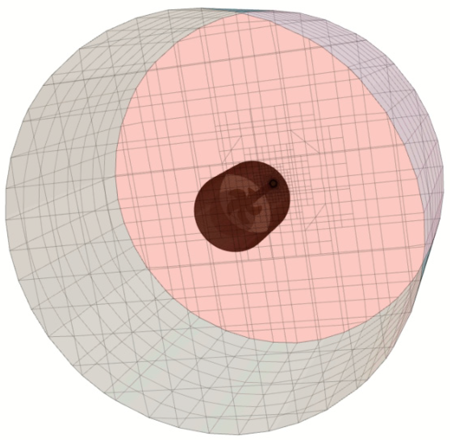
Figure 2.
Grid of the propellers: (a) B series propeller; (b) Original propeller.
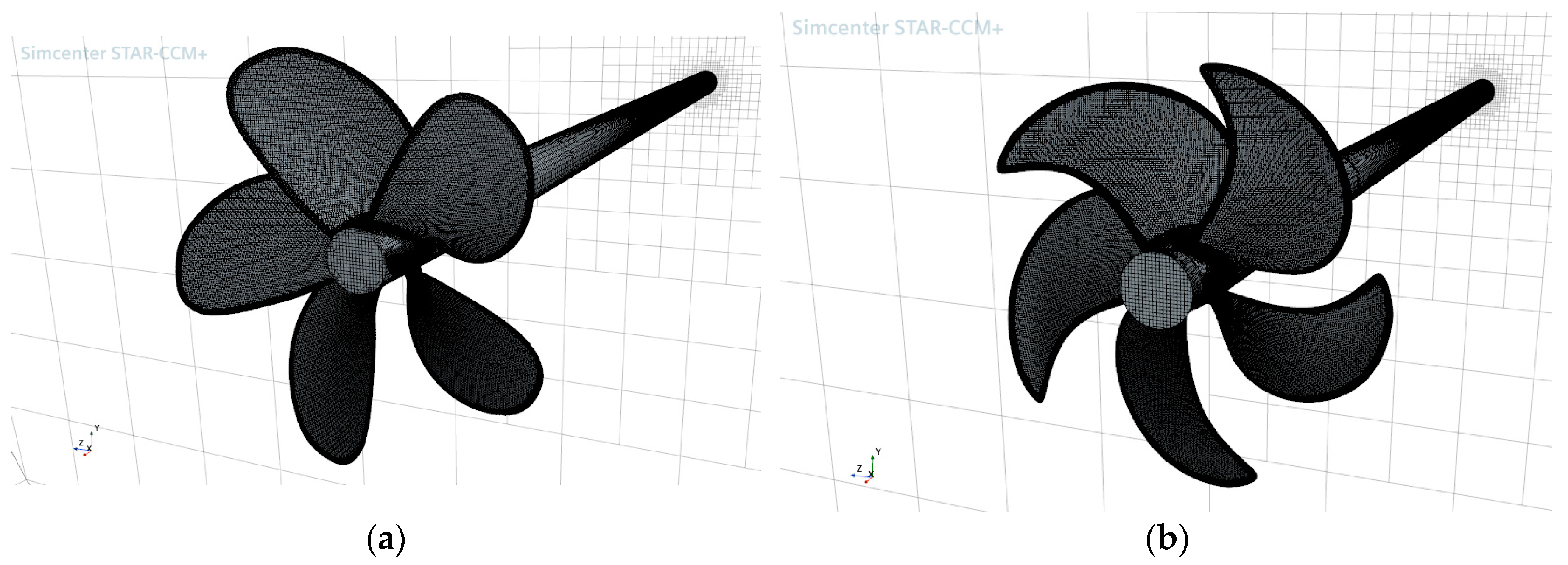
Figure 3.
Results representation: (a) Brake power reduction for one draft; (b) Displacements for three considered drafts and each trim.
Figure 3.
Results representation: (a) Brake power reduction for one draft; (b) Displacements for three considered drafts and each trim.
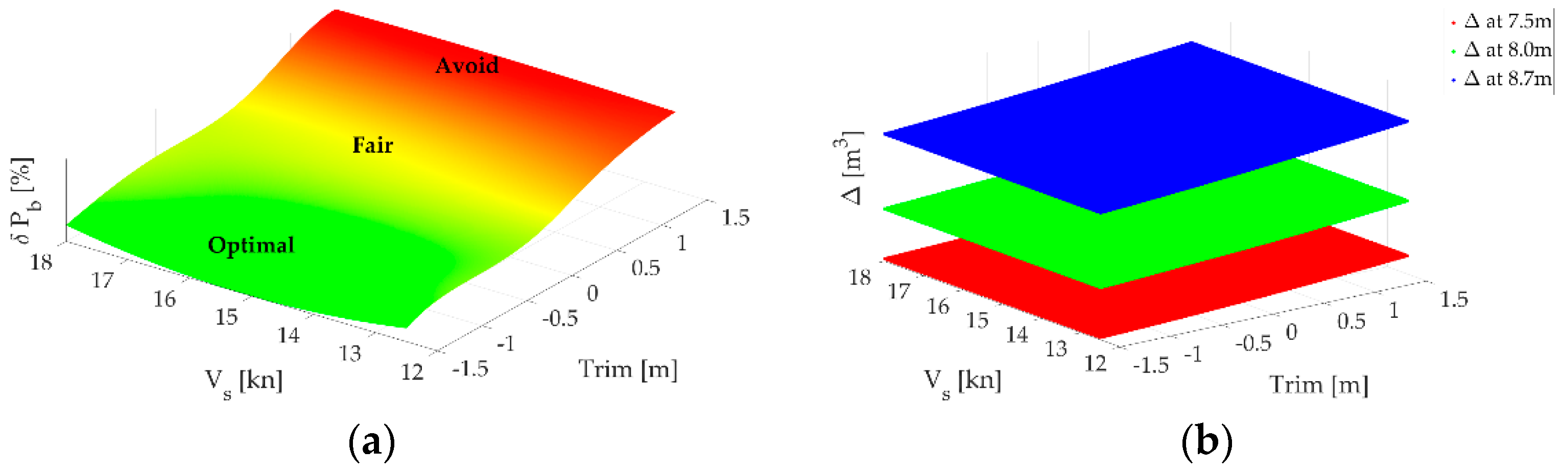
Figure 4.
Results representation: (a) Brake power reduction (δPb) for 120 drafts; (b) Displacements (Δ) for 120 drafts and each trim.
Figure 4.
Results representation: (a) Brake power reduction (δPb) for 120 drafts; (b) Displacements (Δ) for 120 drafts and each trim.
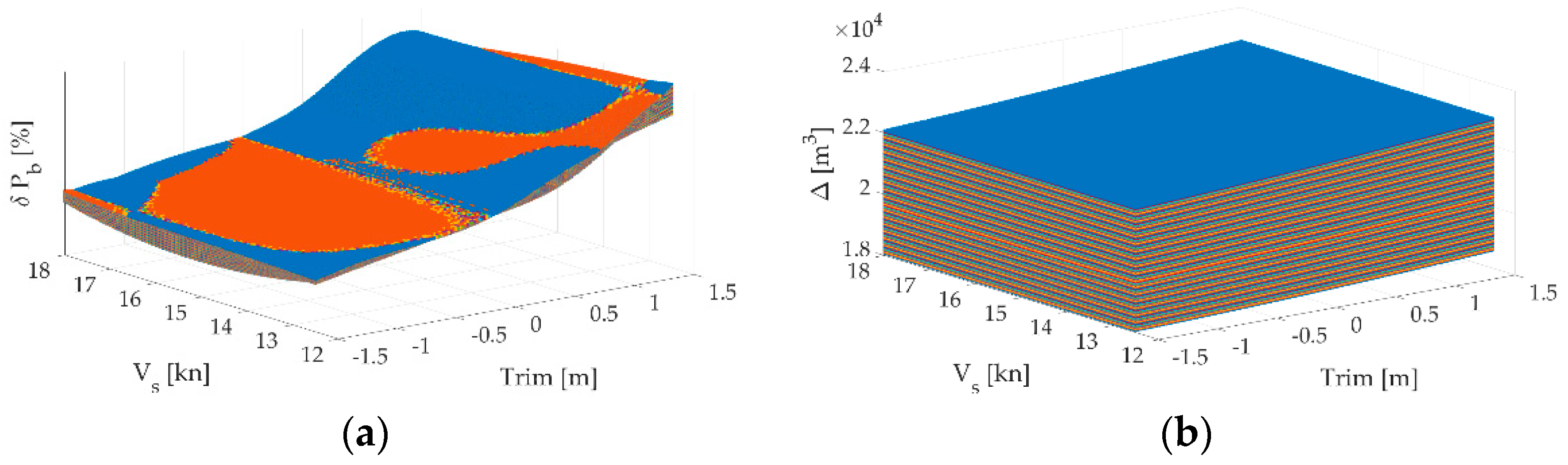
Figure 5.
Results representation for DFOC reduction.
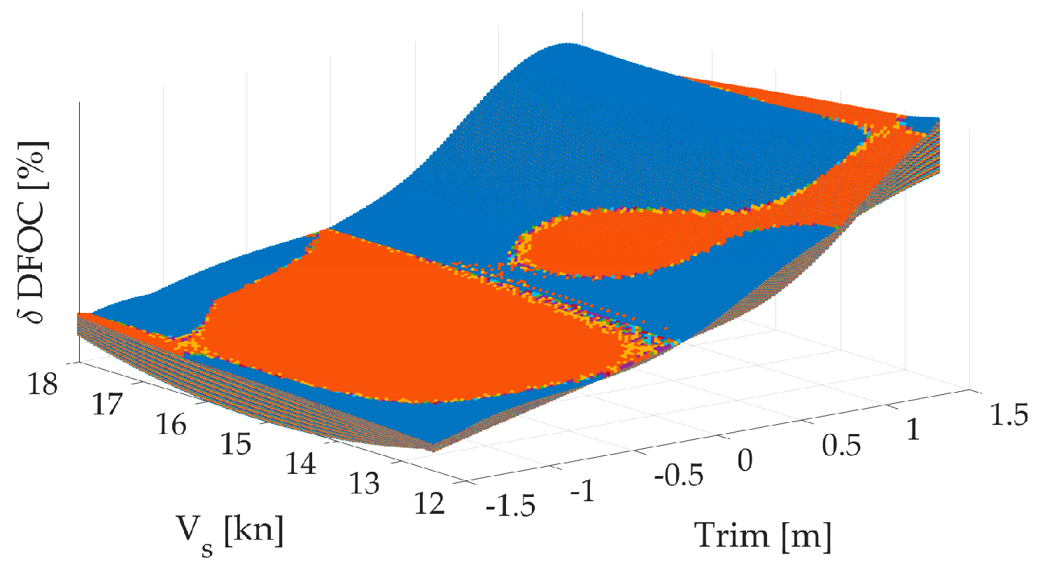
Figure 6.
Illustrated ANN structure of interconnected neurons (circles) and biases (squares).
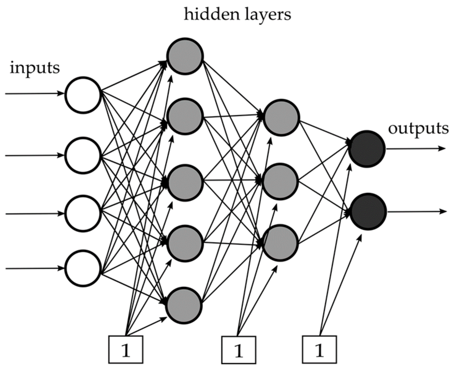
Figure 7.
3D model of the RO-RO ship: (a) bottom view—waterlines; (b) starboard side view—buttocks; (c) aft view—frames.
Figure 7.
3D model of the RO-RO ship: (a) bottom view—waterlines; (b) starboard side view—buttocks; (c) aft view—frames.
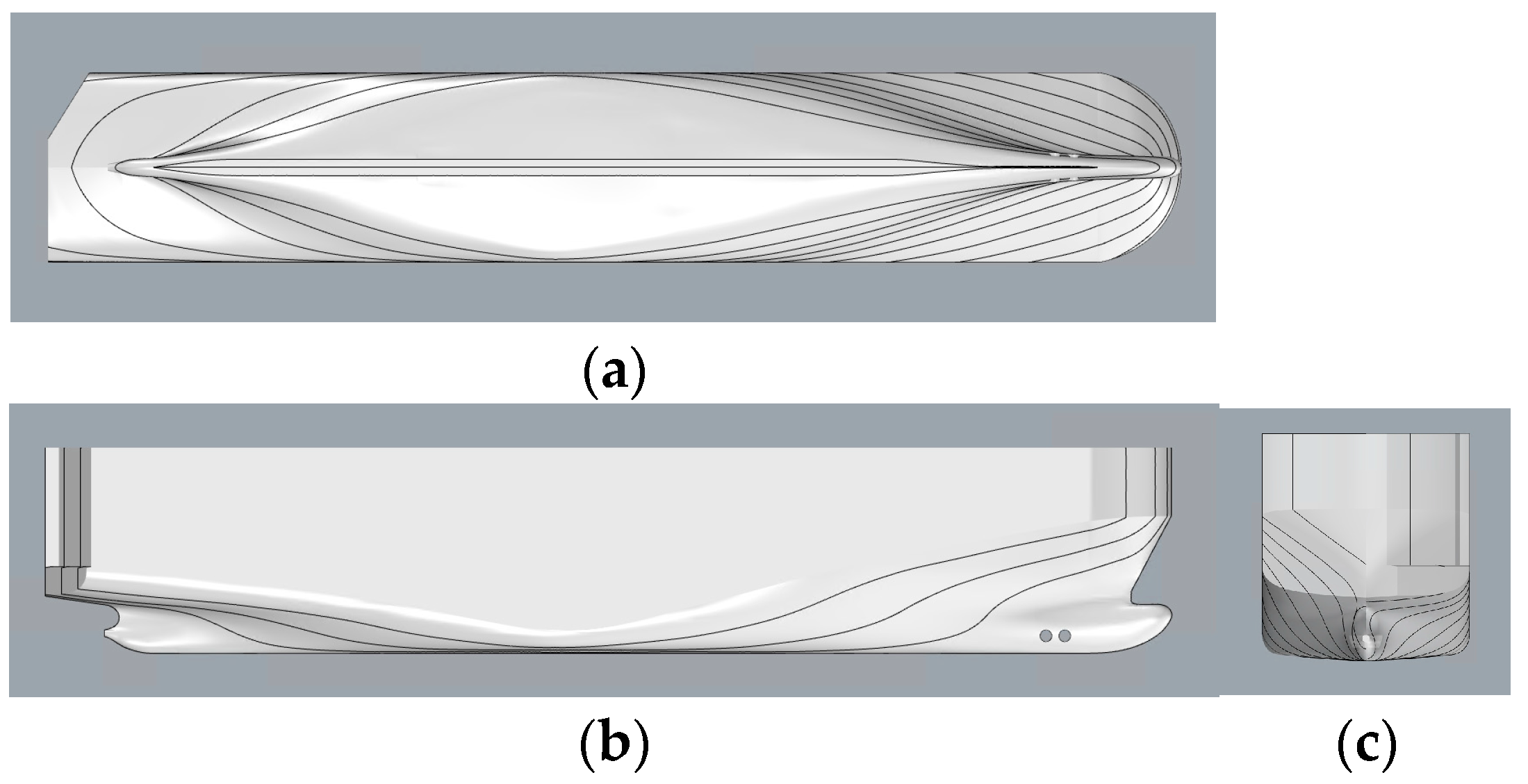
Figure 8.
Propeller; comparison between drawing of 3D modeled propeller (red colored) and reference drawing.
Figure 8.
Propeller; comparison between drawing of 3D modeled propeller (red colored) and reference drawing.
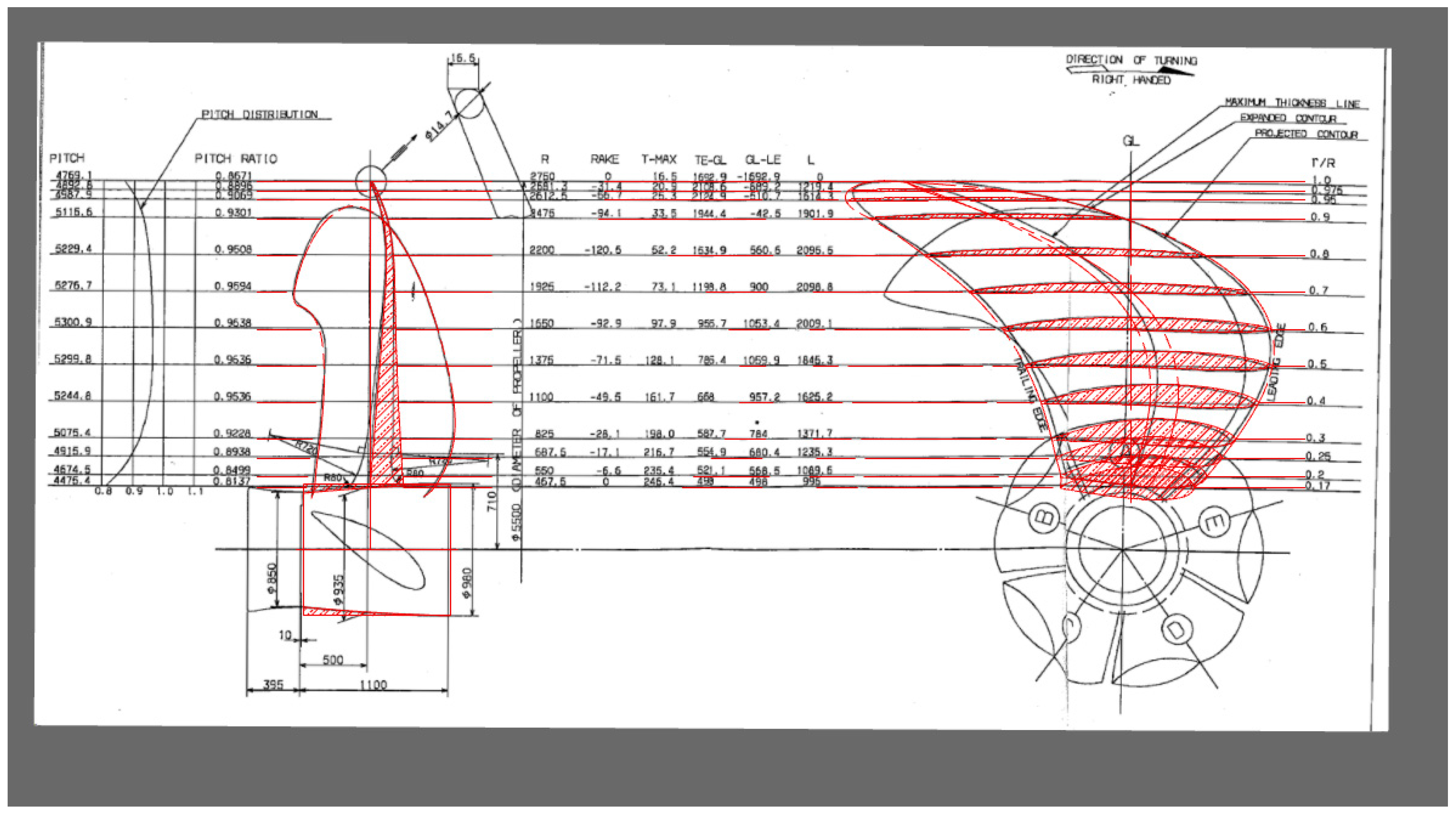
Figure 9.
Propeller and rudder: (a) Original propeller; (b) Rudder.
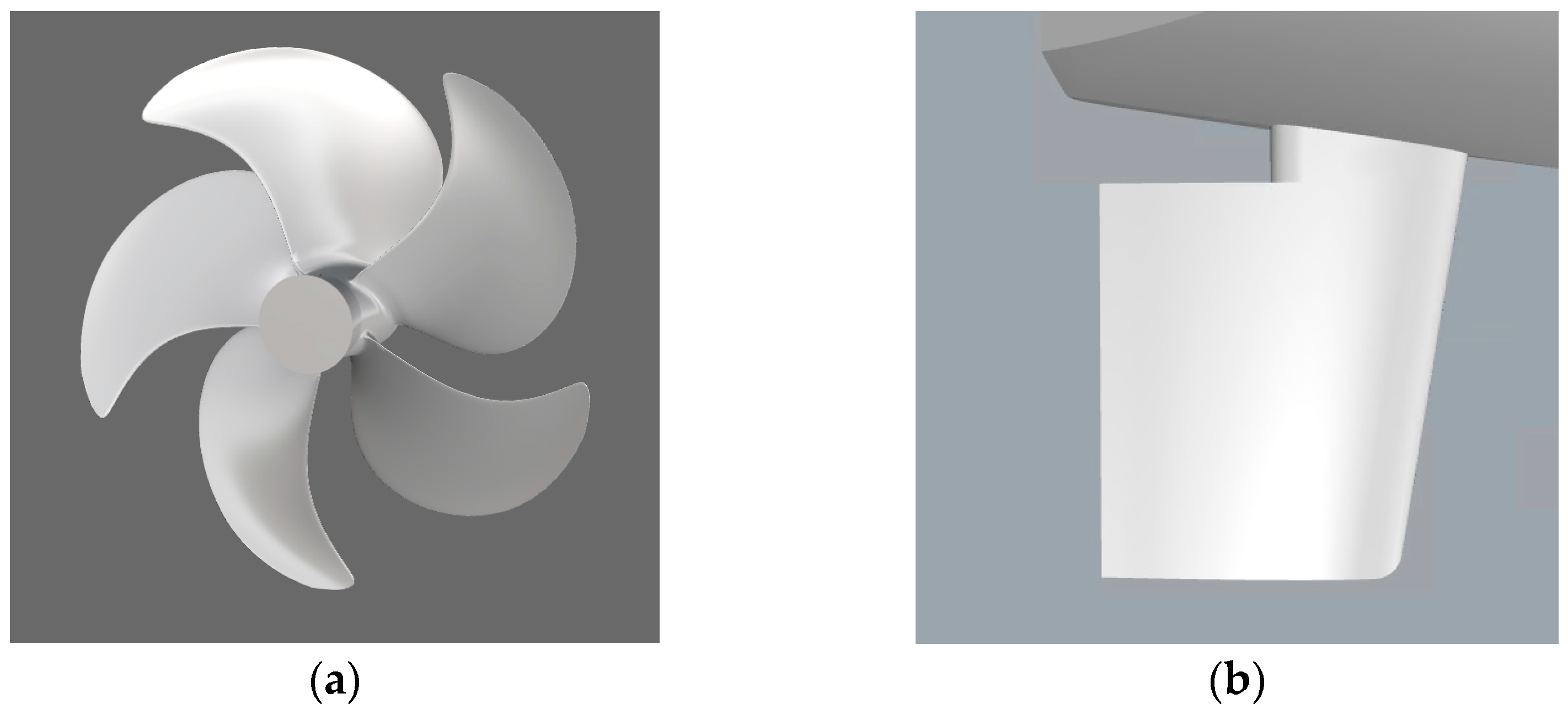
Figure 10.
Propeller characteristics. MM—results based on mathematical model, CFD—results based on OWT CFD simulations: (a) B series propeller; (b) Original propeller.
Figure 10.
Propeller characteristics. MM—results based on mathematical model, CFD—results based on OWT CFD simulations: (a) B series propeller; (b) Original propeller.
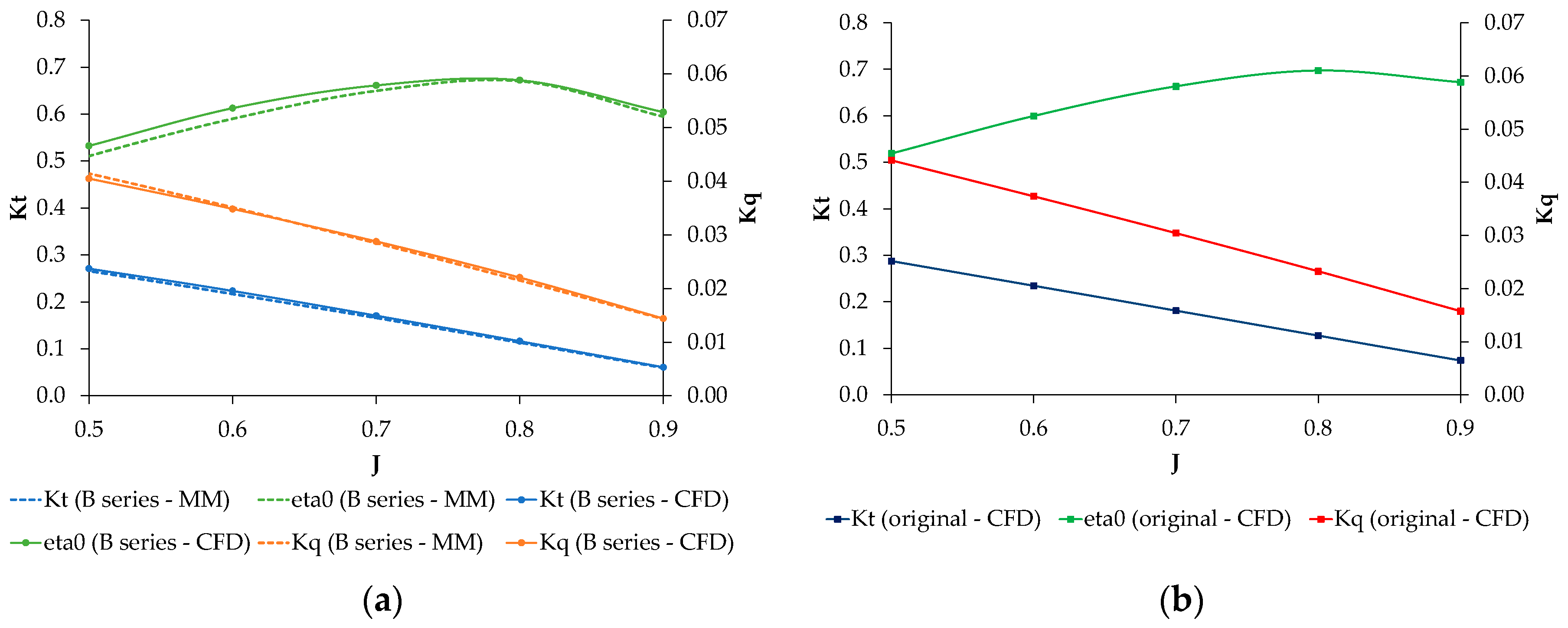
Figure 11.
Domain—Mesh.
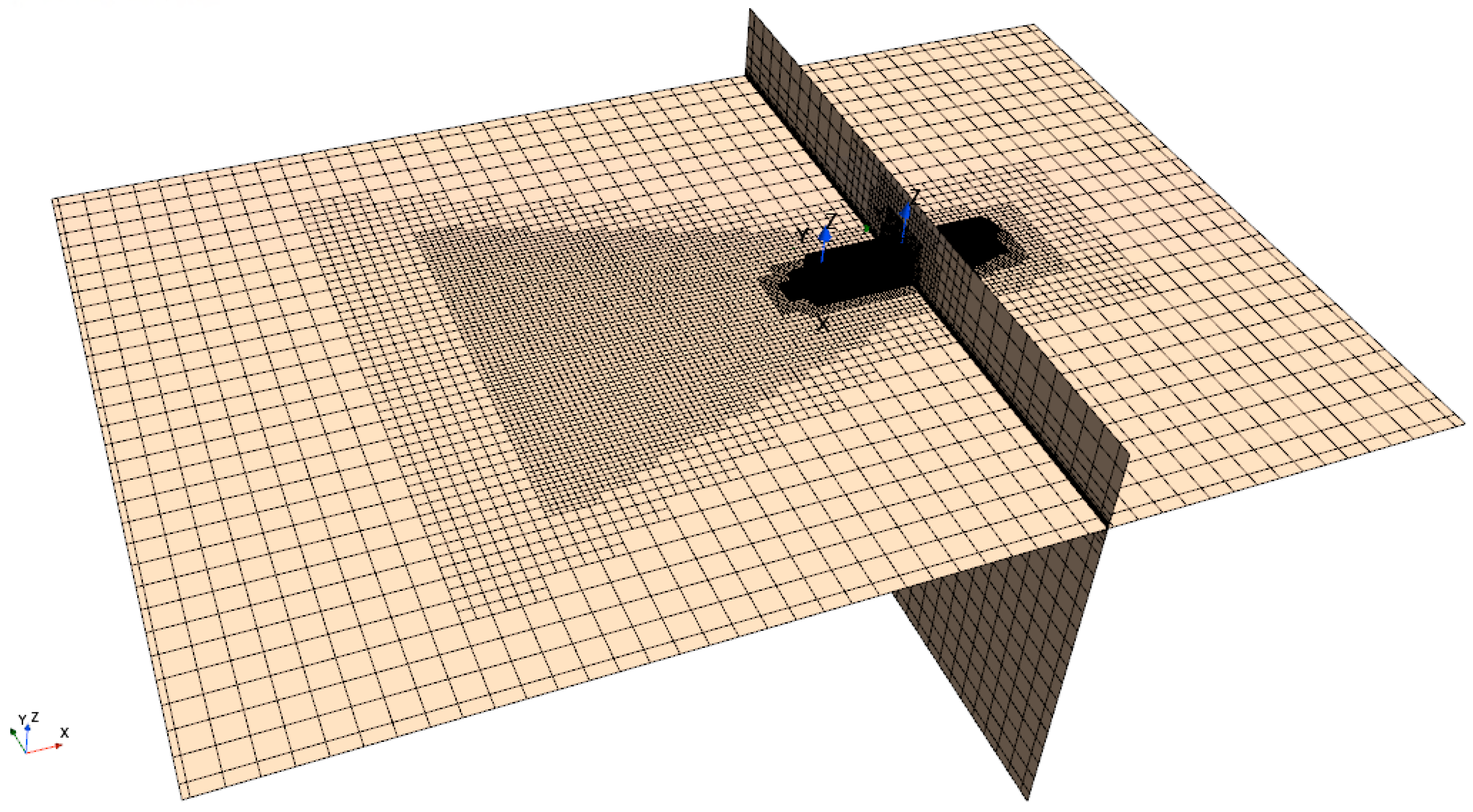
Figure 12.
Refinement zones: (a) Stern part; (b) Bow part.
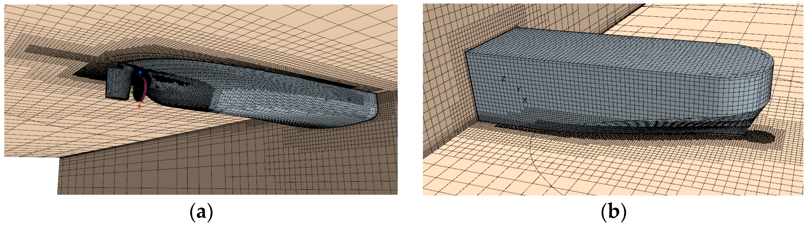
Figure 13.
CFD results for design draft: (a) Pb as a function of Vs; (b) Pb as a function of n.
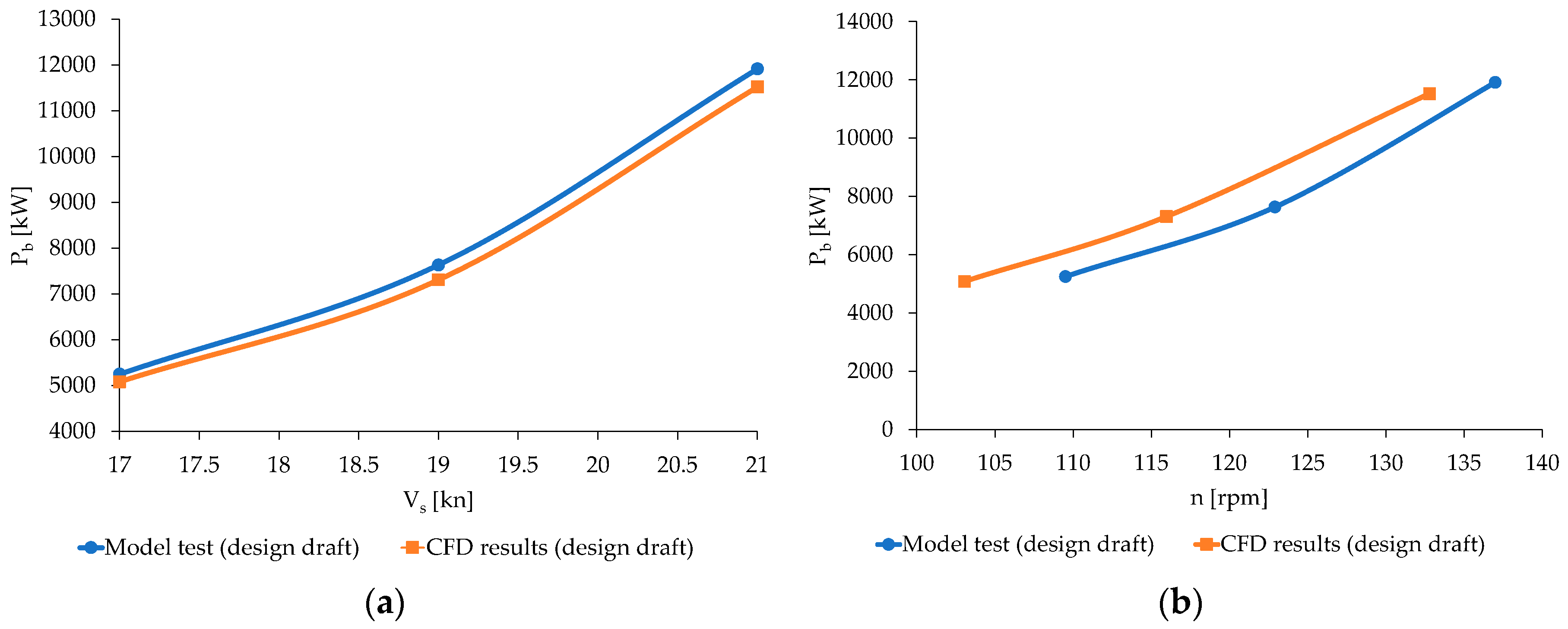
Figure 14.
y+ values: (a) bottom view; (b) bow part—perspective view; (c) starboard side view; (d) stern part—perspective view.
Figure 14.
y+ values: (a) bottom view; (b) bow part—perspective view; (c) starboard side view; (d) stern part—perspective view.
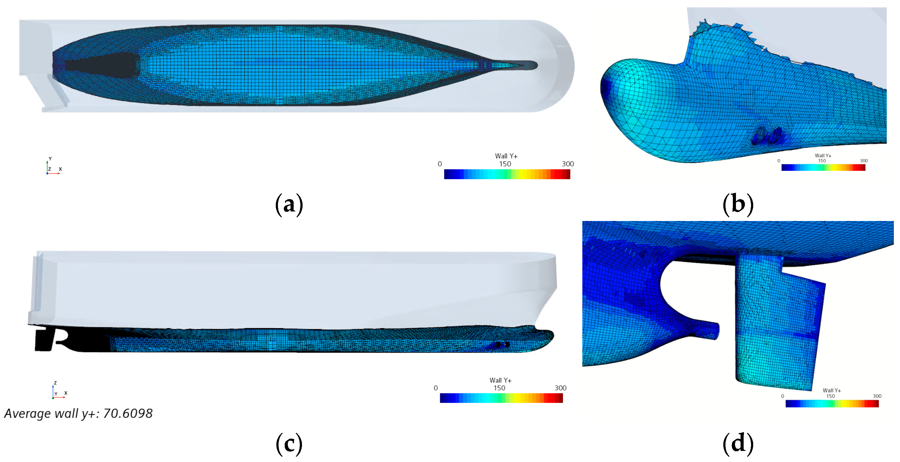
Figure 15.
Brake power reduction: (a) Ts = 7.5m; (b) Ts = 8.0m; (c) Ts = 8.7m.
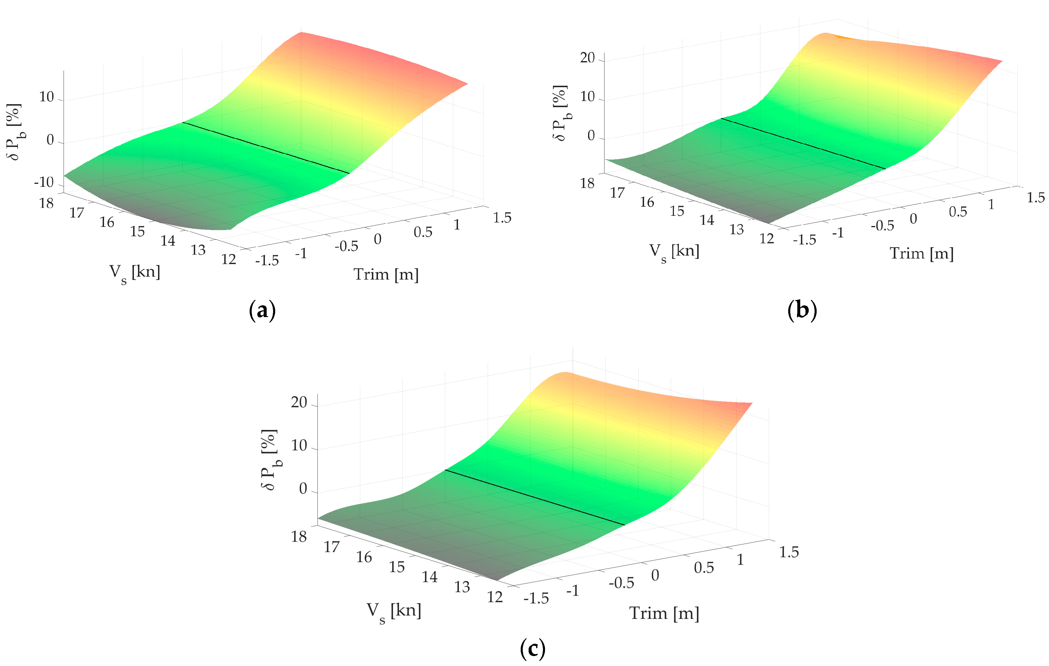
Figure 16.
DFOC reduction: (a) Ts = 7.5m; (b) Ts = 8.0m; (c) Ts = 8.7m.
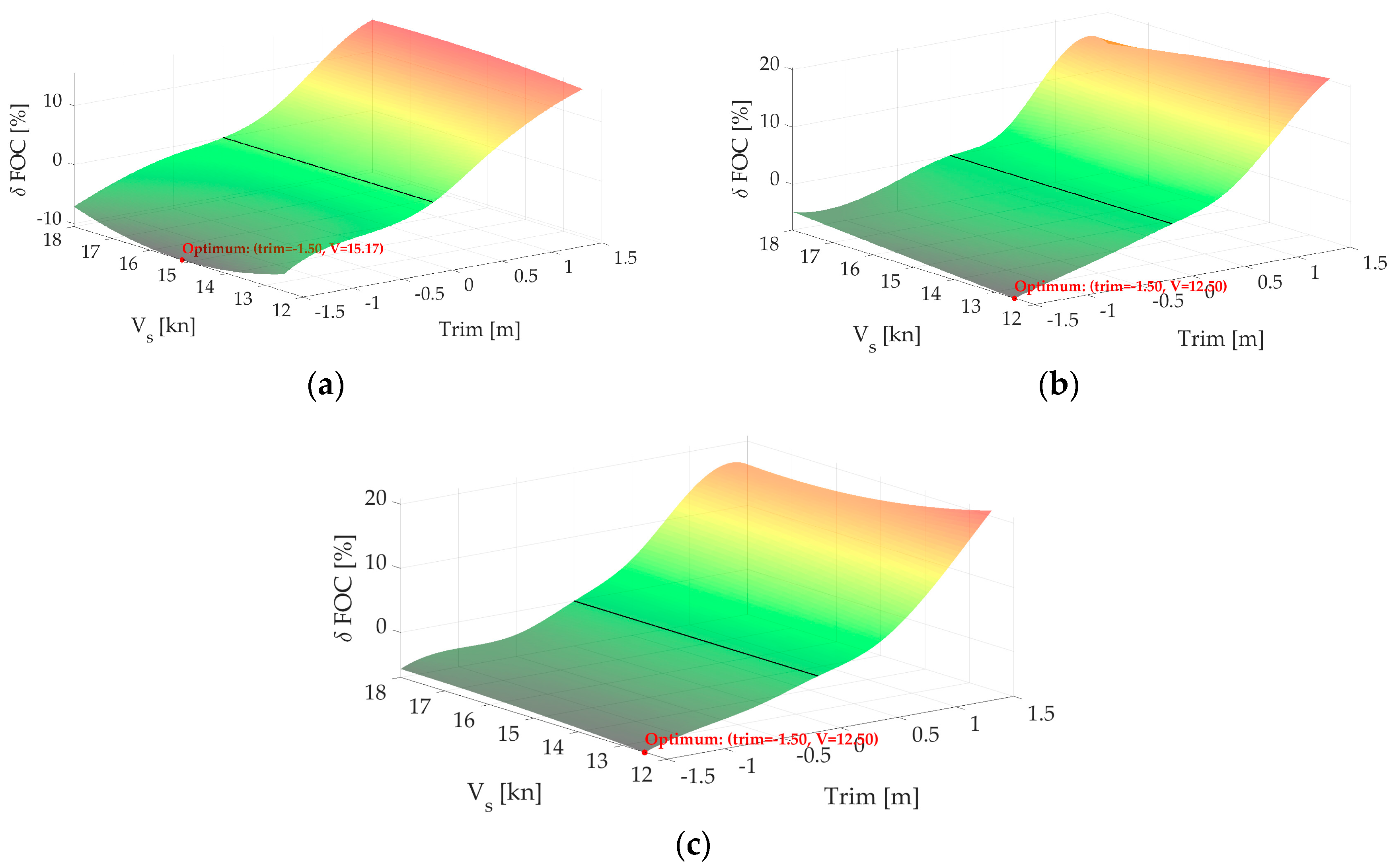
Figure 17.
Wave patterns: (a) Vs=15kn, Ts=7.5m, trim=0m; (b) Vs=15kn, Ts=7.5m, trim=-1.5m.
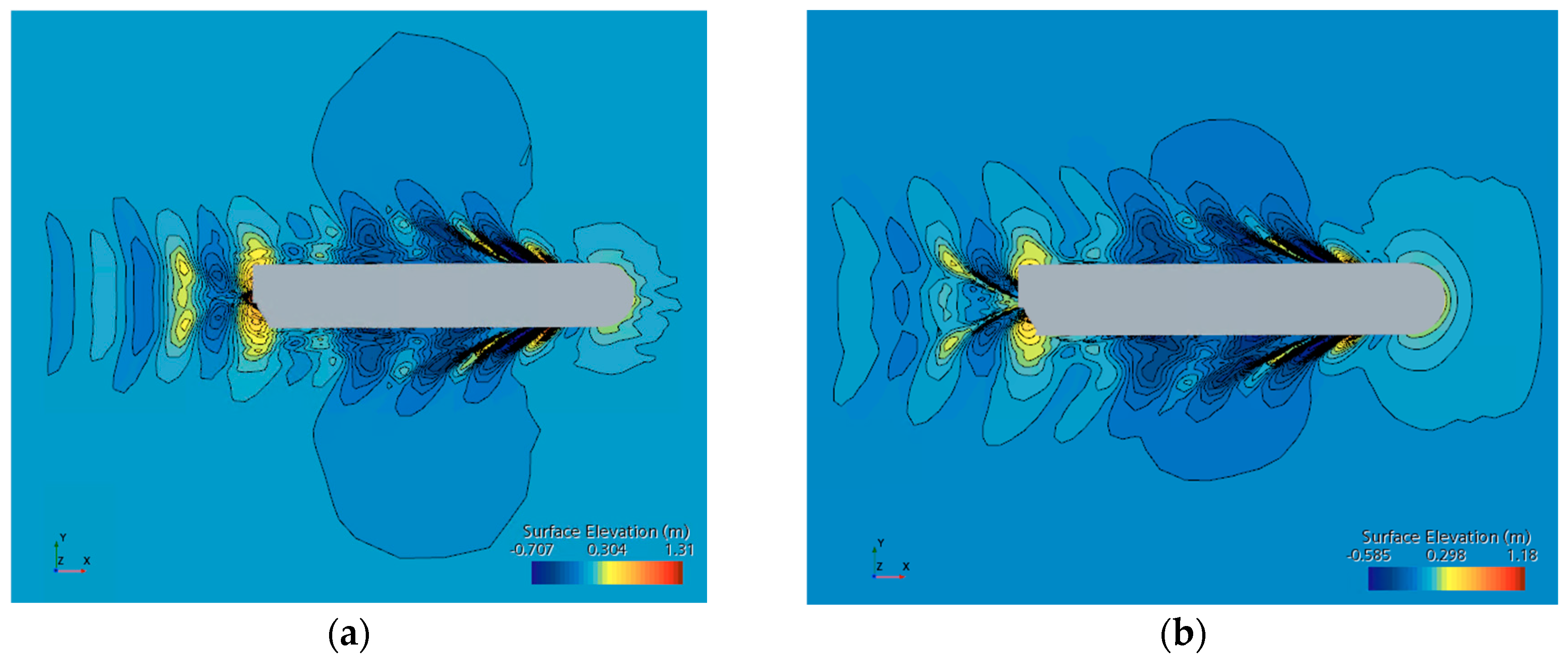
Figure 18.
Free surface cuts (Vs=15kn, Ts=7.5m): (a) Bow part—white colored even keel hull; black line represents free surface elevation for even keel hull, yellow colored (-1.5m) trimmed hull; red line represents free surface elevation for trimmed hull; (b) Stern part—white colored even keel hull; black line represents free surface elevation for even keel hull, yellow colored (-1.5m) trimmed hull; red line represents free surface elevation for trimmed hull.
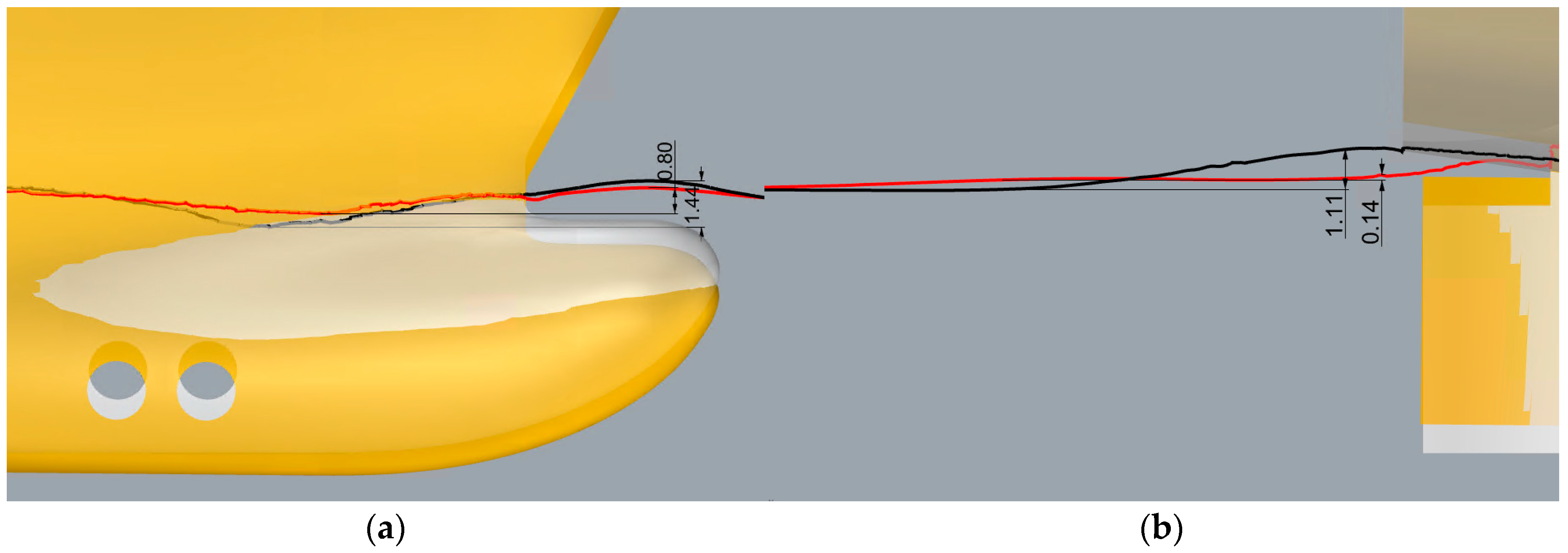
Figure 19.
Configurations of neurons: (a) For brake power and DFOC; (b) For propeller speed.
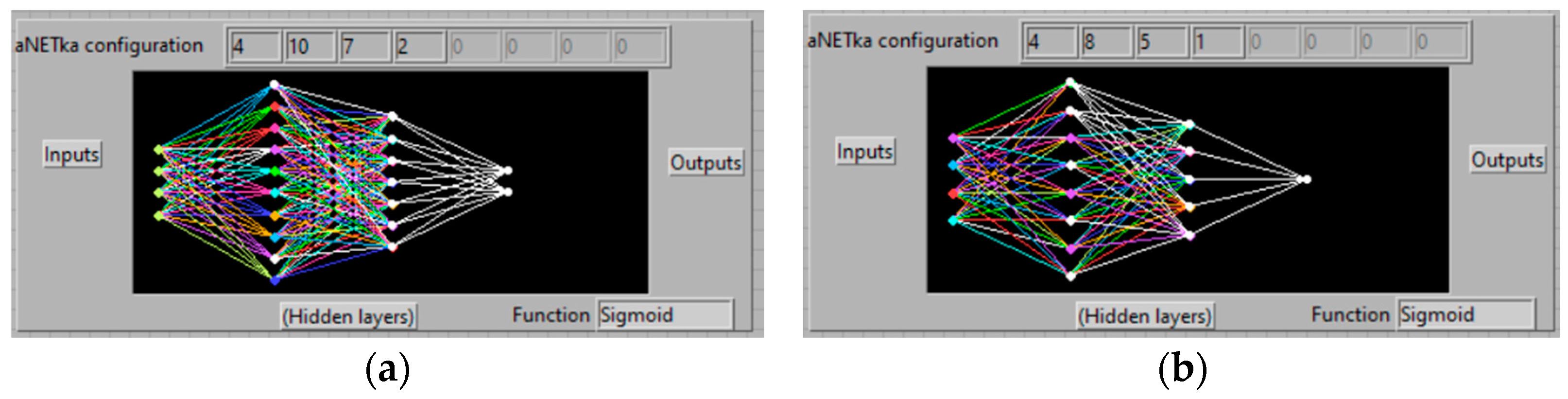
Figure 20.
Application interface design.
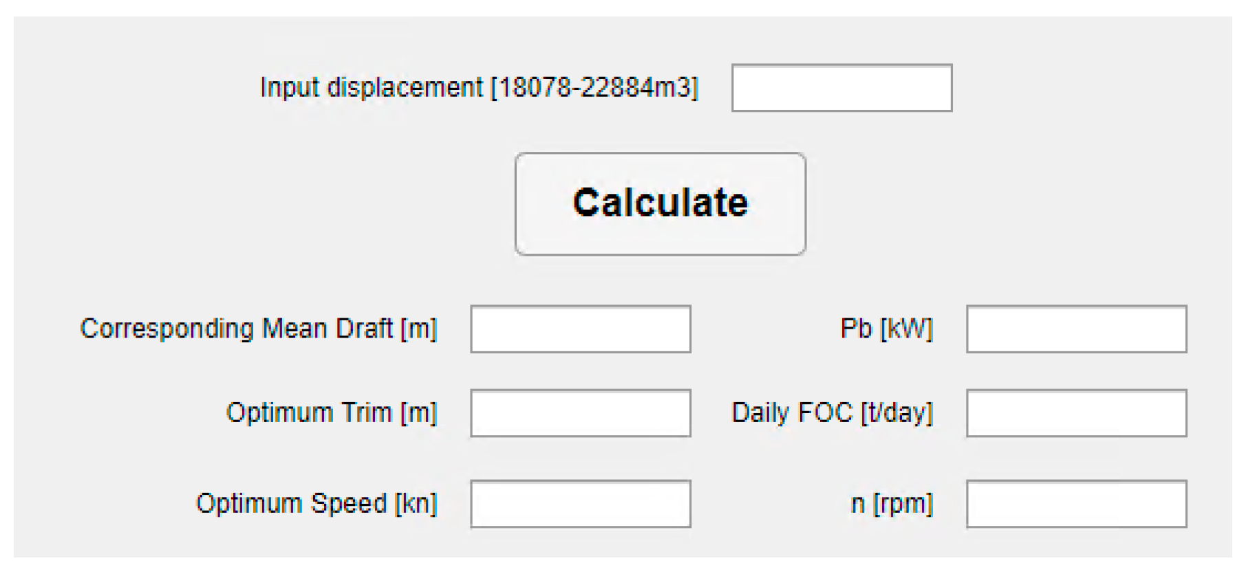
Figure 21.
Wrong input.
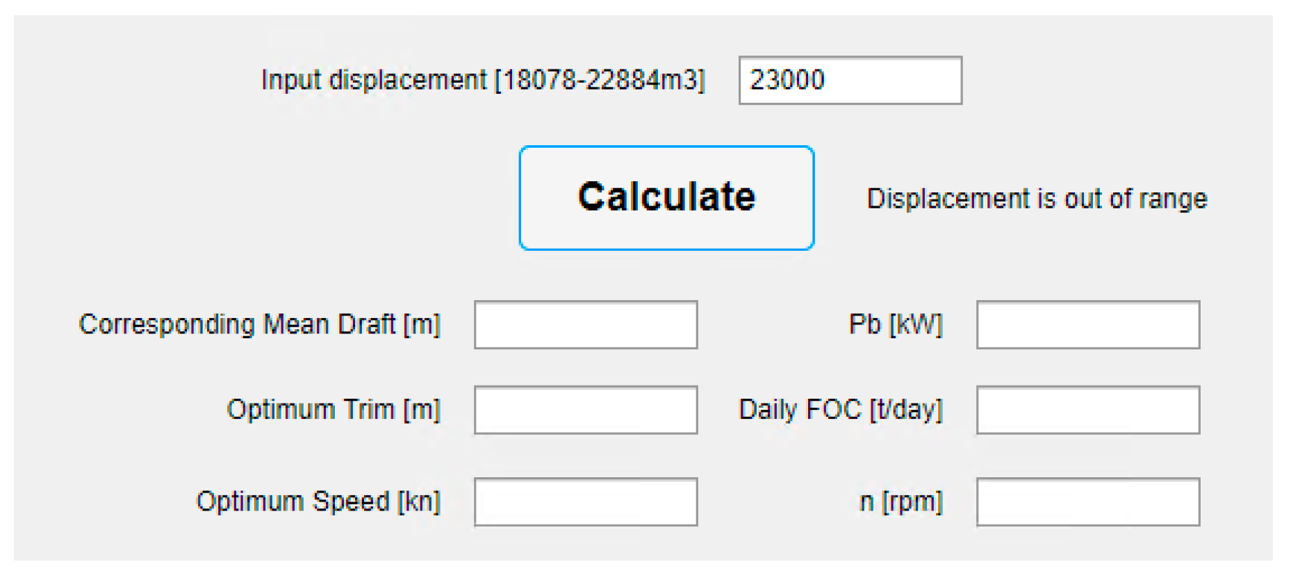
Figure 22.
An example input.
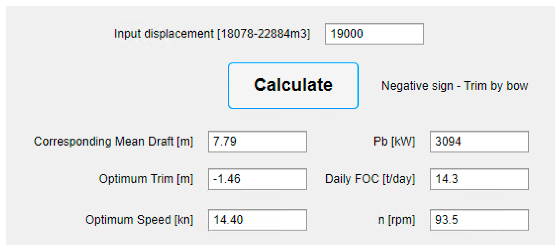
Figure 23.
An example input of displacement that is at the upper limit of the mathematical model’s application.
Figure 23.
An example input of displacement that is at the upper limit of the mathematical model’s application.
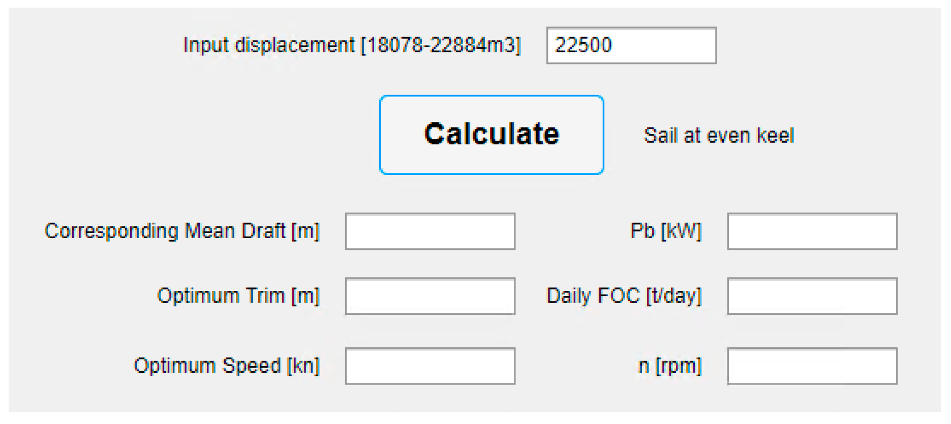

Table 1.
Principal particulars.
| Parameter* | Dimension | Value |
|---|---|---|
| Lpp | [m] | 158 |
| B | [m] | 28 |
| H | [m] | 30.65 |
| Ts | [m] | 7.8 |
* Lpp—length between perpendiculars, B—Breadth, H—Depth, Ts—Draft.
Table 2.
Propeller characteristics.
| Parameter* | Dimension | Value |
|---|---|---|
| D | [m] | 5.5 |
| No. of blades | [-] | 5 |
| BAR | [-] | 0.83 |
| Dhub | [m] | 0.98 |
| Chord length at 0.7Rp | [m] | 2.0988 |
| P/D at 0.7Rp | [-] | 0.9594 |
* D—Diameter, BAR—Blade area ratio, Dhub—Hub diameter, Rp—Propeller radius, P—Pitch.
Table 3.
Comparison between hydrostatics data obtained on the basis of 3D model and Trim % Stability booklet.
Table 3.
Comparison between hydrostatics data obtained on the basis of 3D model and Trim % Stability booklet.
| Ts [m] (trim=0) | CB | Δ | LCB | WS |
|---|---|---|---|---|
| 4 | 0.52% | 0.88% | -0.03% | 0.54% |
| 5 | 0.43% | 0.77% | -0.03% | 0.74% |
| 6 | 0.34% | 0.62% | -0.01% | 0.63% |
| 7 | 0.27% | 0.51% | 0.01% | 0.38% |
| 7.5 | 0.22% | 0.43% | 0.03% | 0.42% |
| 8 | 0.21% | 0.42% | 0.03% | 0.74% |
| 8.7 | 0.23% | 0.42% | 0.03% | 0.79% |
| 9 | 0.31% | 0.40% | 0.03% | 0.82% |
| 10 | 0.14% | 0.31% | 0.03% | 0.87% |
Table 4.
Relative differences between data obtained with mathematical model and results from CFD.
| J | δKT | δKQ | δη0 |
|---|---|---|---|
| 0.5 | 1.9% | -2.3% | 2.2% |
| 0.6 | 2.9% | -0.8% | 2.3% |
| 0.7 | 2.8% | 1.1% | 1.2% |
| 0.8 | 2.7% | 2.4% | 0.2% |
| 0.9 | 2.2% | 0.6% | 1.0% |
Table 5.
Results from CFD analysis for design draft.
| Vs [kn] | Rp [kN] | Rv [kN] | RT’[kN] | t [-] | w [-] | T’ [kN] | Q [kNm] | η0 [-] | n [rpm] | Pb [kW] |
|---|---|---|---|---|---|---|---|---|---|---|
| 17 | 125.454 | 292.216 | 475.936 | 0.1746 | 0.2487 | 576.644 | 466.316 | 0.6736 | 103.1 | 5083 |
| 19 | 178.852 | 366.869 | 622.133 | 0.1579 | 0.2479 | 738.831 | 595.864 | 0.6721 | 116.0 | 7309 |
| 21 | 321.762 | 438.076 | 857.035 | 0.1600 | 0.2458 | 1020.295 | 820.407 | 0.6656 | 132.8 | 11523 |
Table 6.
Grid uncertainty results for thrust.
| Mesh quality | T [kN] |
|---|---|
| Coarse | 544.445 |
| Medium | 539.287 |
| Fine | 535.586 |
| 2.2% |
Table 7.
Propeller speed (n [rpm]): CFD analysis results.
| TRIM BY BOW [m] | EVEN KEEL | TRIM BY STERN [m] | ||||||
|---|---|---|---|---|---|---|---|---|
| Vs [kn] | -1.5 | -1 | -0.5 | 0 | 0.5 | 1 | 1.5 | |
| 7.5m | 12.5 | 82.7 | 83.6 | 84.2 | 85.0 | 86.6 | 87.9 | 88.9 |
| 15 | 97.2 | 98.3 | 99.3 | 100.9 | 102.2 | 103.5 | 105.3 | |
| 18 | 116.8 | 117.9 | 119.0 | 119.7 | 121.1 | 122.6 | 125.1 | |
| 8.0m | 12.5 | 82.4 | 83.1 | 84.0 | 84.7 | 85.7 | 87.7 | 89.5 |
| 15 | 98.3 | 99.3 | 100.2 | 100.7 | 102.3 | 103.5 | 105.8 | |
| 18 | 120.4 | 120.2 | 121.2 | 122.3 | 123.5 | 126.1 | 127.4 | |
| 8.7m | 12.5 | 84.4 | 85.0 | 85.7 | 86.4 | 87.3 | 89.1 | 91.2 |
| 15 | 101.9 | 102.3 | 103.1 | 104.0 | 105.3 | 107.1 | 108.9 | |
| 18 | 125.1 | 125.6 | 126.0 | 127.4 | 129.1 | 131.3 | 132.9 | |
Table 8.
Brake power (Pb [kW]): CFD analysis results.
| TRIM BY BOW [m] | EVEN KEEL | TRIM BY STERN [m] | ||||||
|---|---|---|---|---|---|---|---|---|
| Vs [kn] | -1.5 | -1 | -0.5 | 0 | 0.5 | 1 | 1.5 | |
| 7.5m | 12.5 | 2248 | 2335 | 2370 | 2447 | 2601 | 2739 | 2837 |
| 15 | 3509 | 3665 | 3772 | 3965 | 4130 | 4414 | 4642 | |
| 18 | 5957 | 6187 | 6345 | 6441 | 6667 | 7124 | 7480 | |
| 8.0m | 12.5 | 2155 | 2221 | 2285 | 2357 | 2450 | 2664 | 2882 |
| 15 | 3587 | 3719 | 3818 | 3869 | 4073 | 4352 | 4639 | |
| 18 | 6595 | 6567 | 6750 | 6942 | 7120 | 7879 | 7991 | |
| 8.7m | 12.5 | 2293 | 2353 | 2403 | 2478 | 2564 | 2771 | 3048 |
| 15 | 4018 | 4072 | 4181 | 4303 | 4504 | 4890 | 5113 | |
| 18 | 7531 | 7663 | 7707 | 8003 | 8405 | 9143 | 9361 | |
Table 9.
DFOC [t Fuel/day]: CFD analysis results.
| TRIM BY BOW [m] | EVEN KEEL | TRIM BY STERN [m] | ||||||
|---|---|---|---|---|---|---|---|---|
| Vs [kn] | -1.5 | -1 | -0.5 | 0 | 0.5 | 1 | 1.5 | |
| 7.5m | 12.5 | 10.70 | 11.08 | 11.24 | 11.57 | 12.25 | 12.84 | 13.26 |
| 15 | 16.11 | 16.75 | 17.20 | 18.00 | 18.68 | 19.85 | 20.79 | |
| 18 | 26.22 | 27.18 | 27.83 | 28.23 | 29.18 | 31.09 | 32.58 | |
| 8.0m | 12.5 | 10.29 | 10.58 | 10.86 | 11.18 | 11.59 | 12.52 | 13.46 |
| 15 | 16.43 | 16.98 | 17.39 | 17.60 | 18.45 | 19.60 | 20.78 | |
| 18 | 28.88 | 28.76 | 29.53 | 30.33 | 31.08 | 34.26 | 34.73 | |
| 8.7m | 12.5 | 10.90 | 11.16 | 11.38 | 11.71 | 12.08 | 12.98 | 14.16 |
| 15 | 18.22 | 18.44 | 18.89 | 19.39 | 20.22 | 21.81 | 22.73 | |
| 18 | 32.80 | 33.35 | 33.53 | 34.78 | 36.46 | 39.56 | 40.48 | |
Table 10.
Pressure resistance decrease.
| Vs=15kn, Ts=7.5m | trim=0m | trim=-1.5m |
|---|---|---|
| Rp/Δ·103 [-] | 0.6039 | 0.5127 |
Table 11.
Coefficients A and a for Equations (51) and (52).
| Aj1 | Aj2 | Aj3 | Aj4 | aj |
|---|---|---|---|---|
| 1.39544 | 4.80982 | -1.76190 | -1.30478 | -0.75004 |
| 0.22339 | 3.25659 | -0.04068 | 2.23871 | -1.54100 |
| -2.10995 | 3.49346 | -0.21458 | 1.21715 | -1.63827 |
| 3.03760 | 4.14154 | -2.40221 | 1.04647 | -6.47006 |
| -0.04455 | 0.71422 | 1.58515 | -0.98086 | -0.02750 |
| -1.50944 | 0.27102 | -1.41296 | 1.52488 | 1.06833 |
| -0.97408 | -0.21472 | -0.34123 | -0.58728 | 0.38679 |
| 1.83711 | 2.00358 | -9.92587 | -1.27416 | 3.94278 |
| 0.08588 | 0.39723 | 1.06558 | -0.68159 | -0.95401 |
| -1.45797 | -0.49383 | 3.67284 | -2.41111 | 0.23743 |
Table 12.
Coefficients B and b for Equations (51) and (52).
| Bi1 | Bi2 | Bi3 | Bi4 | Bi5 | Bi6 | Bi7 | Bi8 | Bi9 | Bi10 | bi |
|---|---|---|---|---|---|---|---|---|---|---|
| -3.94741 | -1.10676 | -1.51183 | -3.90542 | 1.28454 | 1.37817 | 1.67905 | 10.13879 | 0.82581 | 2.39590 | 3.05951 |
| -0.83685 | -0.80410 | -0.84916 | -0.74439 | -0.53931 | 1.20460 | 0.17759 | -0.26222 | -0.48840 | -0.58512 | 0.76405 |
| -1.21006 | -1.28977 | -1.53713 | -0.74023 | -1.04296 | 0.87026 | 0.00654 | 0.35832 | -0.85771 | -1.31206 | 0.45529 |
| 0.79825 | -0.92382 | -0.16195 | -3.22868 | 0.48528 | 0.41493 | 0.29515 | -2.64142 | 0.12449 | 1.60271 | 0.59712 |
| -0.83157 | -1.72121 | -1.74315 | -1.78391 | -0.13521 | 2.35956 | 0.85288 | 1.08050 | -0.61823 | -0.66071 | 2.10411 |
| -1.03458 | -1.10428 | -1.25646 | -0.56187 | -0.81983 | 0.76972 | -0.00495 | 0.29741 | -0.77011 | -1.13999 | 0.35562 |
| -0.48851 | -0.49214 | -0.56036 | -0.16494 | -0.22853 | 0.26762 | -0.48143 | 1.41729 | -0.31051 | -1.40889 | 0.36591 |
Table 13.
Coefficients CPb and cPb for Equations (51) and (52).
| CPb1 | CPb2 | CPb3 | CPb4 | CPb5 | CPb6 | CPb7 | cPb |
|---|---|---|---|---|---|---|---|
| -3.60944 | -1.69300 | -1.92004 | -2.15282 | -2.51012 | -1.80109 | -2.08429 | 7.38079 |
Table 14.
Coefficients CDFOC and cDFOC for Equations (51) and (52).
| CDFOC1 | CDFOC2 | CDFOC3 | CDFOC4 | CDFOC5 | CDFOC6 | CDFOC7 | cDFOC |
|---|---|---|---|---|---|---|---|
| -3.60911 | -1.64363 | -2.01584 | -2.11789 | -2.49256 | -1.76852 | -2.02170 | 7.32870 |
Table 15.
Coefficients Pk, Rk, GPb, LPb, GDFOC and LDFOC for Equations (51) and (52).
| Pk | Rk | GPb | LPb | GFOC | LFOC |
|---|---|---|---|---|---|
| 0.75000 | -5.57500 | -0.21915 | 0.00012 | -0.25636 | 0.02980 |
| 0.16364 | -1.99545 | ||||
| 0.30000 | 0.50000 | ||||
| 0.00019 | -3.33586 |
Table 16.
Coefficients A and a for Equation (53).
| Am1 | Am2 | Am3 | Am4 | am |
|---|---|---|---|---|
| 1.60283 | 1.91017 | -1.71984 | 0.23942 | -1.93017 |
| 1.62613 | 2.44722 | -0.17892 | -1.00908 | -3.09041 |
| 1.09543 | 1.09342 | 2.08237 | 0.00351 | -0.00032 |
| -0.17611 | 2.37242 | 0.49469 | 1.22030 | -2.13783 |
| -1.12935 | 5.25606 | -0.88296 | -1.08825 | -0.79561 |
| -1.10799 | -0.07232 | -2.85448 | 0.21127 | 3.80378 |
| -2.76944 | 2.04227 | 4.00000 | -0.90497 | -1.59122 |
| -0.09699 | 1.92632 | 1.05398 | -0.48593 | -0.22092 |
Table 17.
Coefficients B and b for Equation (53).
| Bl1 | Bl2 | Bl3 | Bl4 | Bl5 | Bl6 | Bl7 | Bl8 | bl |
|---|---|---|---|---|---|---|---|---|
| -0.85076 | -0.86022 | -0.92193 | -1.21839 | -1.28573 | 0.12384 | -0.42344 | -0.84941 | 0.72250 |
| -2.21759 | -3.16121 | 1.26550 | -1.20003 | -2.78787 | 4.04679 | -1.95753 | 0.95956 | 3.10950 |
| -1.04299 | -0.99883 | -1.19340 | -1.29826 | -1.50607 | 0.14846 | -0.49616 | -1.15469 | 1.08981 |
| -1.11884 | -0.96068 | -1.18134 | -1.19153 | -1.62624 | 0.20455 | -0.46174 | -1.00754 | 1.02576 |
| -0.43893 | -1.02698 | -1.08333 | -1.41701 | -0.49332 | 1.67727 | 0.33505 | -0.39926 | 1.34012 |
Table 18.
Coefficients C and c for Equation (53).
| Cn1 | Cn2 | Cn3 | Cn4 | Cn5 | cn |
|---|---|---|---|---|---|
| -2.44334 | -5.02627 | -2.91111 | -2.88484 | -2.67661 | 6.86984 |
Table 19.
Coefficients Ps, Rs, Gn and Ln for Equation (53).
| Ps | Rs | Gn | Ln |
|---|---|---|---|
| 0.75000 | -5.57500 | -1.41852 | 0.01782 |
| 0.16364 | -1.99545 | ||
| 0.30000 | 0.50000 | ||
| 0.00019 | -3.33987 |
Disclaimer/Publisher’s Note: The statements, opinions and data contained in all publications are solely those of the individual author(s) and contributor(s) and not of MDPI and/or the editor(s). MDPI and/or the editor(s) disclaim responsibility for any injury to people or property resulting from any ideas, methods, instructions or products referred to in the content. |
© 2024 by the authors. Licensee MDPI, Basel, Switzerland. This article is an open access article distributed under the terms and conditions of the Creative Commons Attribution (CC BY) license (http://creativecommons.org/licenses/by/4.0/).
Copyright: This open access article is published under a Creative Commons CC BY 4.0 license, which permit the free download, distribution, and reuse, provided that the author and preprint are cited in any reuse.


