

Submitted:
17 June 2024
Posted:
19 June 2024
You are already at the latest version
Abstract
Every year, the Montreal police are confronted with countless crimes committed by criminals. These crimes affect the quality of life of city residents and impose a socio-economic burden on the city. In this study, we conduct a comparative analysis based on several machine learning algorithms to develop a model to predict the crime category in Montreal. The performance of algorithms such as eXtreme Gradient Boosting (XGBoost), Decision Trees (DT) and Random Forest (RF) were analyzed. The performance analysis takes into account the performance metrics such as precision, accuracy, recall and F1-score. This analysis was based on crime data in Montreal from 2015 to 2023. This data is characterized by a strong imbalance between crime categories. To address the data imbalance problem, a data balancing approach based on the SMOTE-ENN algorithm was adopted. In the exploratory data analysis phase, temporal trends by crime category were highlighted. The results of the analysis showed that the XGBoost algorithm outperformed the other two. Specifically, the XGBoost algorithm achieves an accuracy of 92%, while DT and RF achieve an accuracy of 86% and 84%, respectively. As a result, XGBoost was deployed via a web application using the Flask and Swagger UI Python frameworks. This study provides the Montreal police with an effective tool to better utilize their resources in fighting crime. In addition, policymakers in the city of Montreal can use this tool to identify high-risk areas and give them more attention.
Keywords:
crime prediction
; machine learning
; XGBoost
; Decision Trees
; Random Forest
; data imbalance
; Montreal
1. Introduction
Criminal activities in urban areas represent a major challenge worldwide. They have a significant impact on the quality of life of urban residents and impose a heavy socioeconomic burden [1]. Montreal, one of Canada’s largest cities, is no exception. The City of Montreal Police Department is constantly faced with a variety of criminal activities every year [2]. Given this situation, it is important to take a proactive approach to optimize the allocation of police resources and increase the safety of Montrealers. In this context, the use of artificial intelligence, particularly machine learning, emerges as a promising strategy to predict and better manage incidents related to criminal activities [3,4].
Given the scale and complexity of crime in Montreal, the development of advanced predictive systems is critical to predict different types of crime. The introduction of such technologies would significantly improve the responsiveness and effectiveness of police interventions while strengthening crime prevention measures. The main challenge lies in the processing and detailed analysis of large data sets on criminal activities, which are characterized by a significant imbalance between crime categories. The reliability of forecasting tools can be affected by this imbalance, increasing the possibility of forecast bias.
This research makes a significant contribution to the literature on public safety and the application of machine learning in urban crime management through the following focuses:
- Development of a predictive model: We present an innovative machine learning-based model that uses the XGBoost algorithm to predict crime patterns in Montreal. Our study analyzes data on crimes committed in Montreal from 2015 to 2023 and shows that our model based on the XGBoost algorithm outperforms other methods such as DT and RF.
- Classifier performance evaluation: An in-depth evaluation of the various machine learning algorithms was carried out, highlighting the effectiveness of the XGBoost algorithm compared to its competitors (DT and RF) in terms of precision, accuracy, recall and F1-score.
- Real-time prediction web application: Providing an innovative web application that integrates the XGBoost prediction model developed with Python Flask and Swagger UI to provide users with an interactive platform for entering data and receiving predictions on crime categories.
- Applying supervised learning to a new crime analysis data set: For the first time in Montreal, supervised learning is being applied to crime data to develop a tool that will help law enforcement agencies optimize the management of their resources and fight crime more effectively.
The remainder of this article is organized as follows: Section 2 is dedicated to reviewing relevant research; Section 3 provides an overview of the data used in this study; the methodology used to predict crime categories in Montreal is described in Section 4; the results of the developed prediction models and their analysis are presented in Section 5; the deployment of the most effective prediction model is discussed in Section 6; and finally, the conclusions and research prospects are presented in Section 7.
2. Related Work
The use of artificial intelligence (AI) to combat urban crime is becoming increasingly popular among scientists around the world. Numerous research and analyzes have examined the possibilities of artificial intelligence and machine learning in anticipating and controlling criminal behavior, highlighting their ability to revolutionize law enforcement practices and improve public safety. This section presents important contributions to this field, with a focus on developments and strategies to successfully combat urban crime.
[5] apply a classification-based strategy to predict crime categories. To accomplish this task, the authors evaluate and compare the performance of two classification algorithms: the RF and the Support Vector Machine (SVM). The development of their classification model is based on the analysis of the "Crime and Communities" dataset available in the University of California, Irvine (UCI) machine learning database. The obtained results show that the RF algorithm outperforms the SVM in terms of crime classification accuracy, achieving a rate of 99%.
The research conducted by [6] led to the development of a machine learning model dedicated to predicting crime categories in a specific geographical area. To this end, the authors implemented a methodology to evaluate and compare the effectiveness of two classification algorithms: Decision Trees and Naive Bayes. Their study uses data on crimes committed in the city of Chicago. The performance evaluation of these algorithms focused on the nine most relevant variables in the data set. This comparative analysis showed that the Decision Tree algorithm outperformed the Naive Bayes algorithm and achieved an accuracy of 91.68%.
The study by [7] presents a collaborative approach called assemble-stacking-based crime prediction method (SBCPM) that leverages SVM algorithms to improve the accuracy of crime prediction in India. It combines multiple classifier predictions to handle the complex nature of crime dynamics and leverages MATLAB for implementation. The authors used the NCRB (National Crime Record Bureau) Indian criminal records data set. Compared to single models such as J48, SMO, Naïve Bayes Bagging, and RF, the ensemble method shows superior performance with significant improvements in prediction accuracy (99.5% on test data) and correlation coefficients. This method outperforms previous efforts by providing more accurate predictions, particularly for violent crime datasets, and fits well with criminological theories.
The research of [8] led to the development of a crime prediction model for Dubai using open source software to evaluate the performance of various machine learning algorithms: RF, KNN, SVM, ANN, Naïve Bayes, and Decision Tree. The authors used a data set containing samples of crimes committed in the Emirate of Dubai (United Arab Emirates). Their comparative study shows that the KNN algorithm stands out in its performance and outperforms the other tested methods with an accuracy of 78.47%.
[9] explores the application of machine learning algorithms to crime prediction to help police departments effectively allocate resources to combat crime in urban areas. By analyzing over 6 million records from the Chicago Police Department’s CLEAR system, the study evaluated various machine learning algorithms, including RF, K-Nearest Neighbors, AdaBoost, and Neural Networks, to predict crime severity and possible arrests. Among the algorithms evaluated, the Neural Network demonstrated the highest accuracy at 90.77%, providing valuable insights into the potential of machine learning for crime prediction in big cities.
The study by [10] aims to automate the identification of legal crimes in crime reports using the San Francisco Crime dataset, which includes data from 2003 to 2015 and focuses on the 15 most common of 39 crime types with a total of 280,000, focused data sets. Before using a RF classifier, a preprocessing scheme was applied that included data categorization, standardization, and oversampling. The methodology achieved an average accuracy of 86.5% with comparable precision, recall, and F-score, along with an AUC of 0.98 and an MSE of 0.1 in the regression analysis.
In [11], the authors use supervised learning techniques to predict criminal activities. The study analyzes a 12-year data set of criminal incidents in San Francisco and initially applies DT and KNN algorithms that provide modest prediction accuracies. Then, incorporating RF as an ensemble method and AdaBoost improves the prediction accuracy. Performance evaluation using log loss, which penalizes false predictions, demonstrates the effectiveness of random undersampling with the RF algorithm in eliminating class imbalance, resulting in a prediction accuracy of 99.16% and a log loss of 0.17%.
In [12], the authors use data mining and the KNN algorithm to assess and identify crime trends that significantly impact community safety. Their study focuses on addressing daily security challenges such as hijackings, kidnappings, and harassment that people may face due to unreliable route assessments provided by navigation tools such as Google Maps. By applying clustering techniques and primary and secondary data, the study assesses crime rates in Bangladesh and provides predictions on various crimes and their locations. Other machine learning algorithms, such as Naive Bayes and Linear Regression, have been contrasted with the KNN algorithm. The performance analysis results show that the KNN algorithm outperforms the other two and achieves an accuracy of 76.92%. The analysis enables the development of a method for determining safe routes and improves a person’s ability to avoid high-risk areas and reach their destination safely.
In [13] conducted a comprehensive analysis using a range of machine learning models such as Logistic Regression, SVM, Naive Bayes, KNN, DT, Multilayer Perceptron (MLP), RF, XGBoost, and time series analysis using Long Short-Term Memory (LSTM) and Autoregressive Integrated Moving Average (ARIMA) techniques to improve crime data prediction. The study found that LSTM performs effectively in time series forecasting, as evidenced by its Root Mean Square Error (RMSE) and Mean Absolute Error (MAE). Through exploratory analysis, the research identified more than 35 crime types and observed an annual decline in crime rates in Chicago but a slight increase in Los Angeles. Future projections suggest a slight increase in crime rates in Chicago with possible subsequent declines, while Los Angeles is expected to see a significant decline, according to the ARIMA model. These findings facilitate the early detection of crime, the location of high-risk areas, the prediction of future crime trends, and provide valuable insights for the further development of police practices and strategies.
[14] introduces a model that uses three established machine learning algorithms - Naive Bayes, RF, and Gradient Boosting Decision Trees - to predict the probability of the ten most common crimes, which account for 97% of recorded incidents. These crimes are divided into two main groups: violent and non-violent. Through exploratory data analysis (EDA) of a crime dataset, the model identifies patterns and trends. Performance evaluations show accuracy rates of 65.82% for Naive Bayes, 63.43% for Random Forest, and 98.5% for Gradient Boosting Decision Trees. Notably, the Gradient Boosting Decision Tree algorithm shows superior performance in both precision and recall metrics. The study concludes that the Gradient Boosting Decision Tree model is the most efficient for crime prediction. It provides critical insights and enables law enforcement agencies to improve resource allocation, improve crime prediction, and better serve the community. The research uses the San Francisco crime data set.
Although the previous studies have made significant progress, our current work is distinguished by its focus on crime categories in the city of Montreal to improve public safety. Our approach uses supervised machine learning algorithms to develop a web-based application for predicting crime categories in Montreal.
Table 1 briefly summarizes these studies based on their focus, data used, models evaluated and key findings.
3. Data Overview
This section provides an overview of the datasets used in this study. Collecting and describing data will be the two main topics of discussion.
3.1. Data Collection
The dataset used in this research includes records of criminal activity in the City of Montreal from 2015 to 2023. The Montreal City Police Service (MCPS) used incident reports to compile these records. The dataset has been updated and anonymized to address privacy concerns and protect personal information. It covers a wide range of criminal activity in Montreal, from minor property crimes to violent crimes. The dataset is accessible via the City of Montreal web portal [15] under Attribution (CC-BY 4.0) [16].
3.2. Data Description
The following Table 2 lists the attributes (columns) corresponding to each entry in the dataset used for this study.
In the Table 2, the crime category attribute denotes the target variable. Figure 1 illustrate the distribution of each category with respect to the target variable using a pie chart.
Figure 1 shows a pronounced discrepancy between the majority and minority classes, indicating the need for a data balancing approach to improve the effectiveness of the prediction model. The methodological part of this study explains in more detail how this challenge can be overcome.
4. Methodology
In this section, we outline the methodology used to model the prediction of criminal activity in Montreal and present it as a multi-class classification challenge. Criminal activity is divided into six different categories: Theft from/in Motor Vehicle, Break and Enter, Mischief, Motor Vehicle Theft, Robbery, and Offenses Causing Death.
Our research is based on a comprehensive evaluation of various classification algorithms, including XGBoost, DT and RF. The goal of this evaluation is to determine which classification algorithm produces the most accurate results (in terms of precision and F1-score) when applied to a dataset of criminal activity in Montreal.
Therefore, in the next part of this section, we will detail the steps to develop the model to predict criminal activity in Montreal. These steps include several key phases: data preprocessing, feature selection, exploratory data analysis, the development of the predictive model, and the validation and evaluation of the model.
4.1. Data Preprocessing
This subsection refers to the critical phase of data preprocessing before analysis. It includes several steps such as extracting new features from the Date column, removing redundant data, grouping variables into numeric and categorical, dealing with missing data, encoding categorical variables and dealing with imbalanced datasets.
4.1.1. Temporal Extraction: Weekday, Day, Month, Year
Our dataset contains a Date column in the format YYYY-MM-DD. We use the to_datetime function from the Python Pandas library [17] to convert this column into a format that our prediction model can interpret. This conversion facilitates the extraction of additional temporal features, including day of the week, day, month, and year. Such a transformation improves the usability of the Date column and allows the prediction model to better understand and use temporal information.
4.1.2. Redundant Data Removal
In this phase, we perform a transformation aimed at removing redundant data from our dataset. After the additional columns Weekday, Day, Month, and Year are successfully extracted from the Date column, retaining this column is no longer necessary. Therefore, the Date column is identified as redundant and is subsequently removed from our dataset using the drop method provided by the Python Pandas library.
4.1.3. Categorizing Variables: Numerical and Categorical
In this phase, we categorized attributes according to their type – numerical or categorical. Specifically, attributes labeled as object type were classified as categorical variables. Conversely, attributes corresponding to the int64 and float64 data types were identified as numeric variables. To facilitate this classification, we used the select_dtypes function from the Python Pandas library.
4.1.4. Handling Missing Values
In this phase, we address the issue of missing data in our dataset. For each attribute, we determine both the number and percentage of missing data. Table 3 provides a summary of the missing data for each attribute, indicating both the amount and percentage of missing values.
Looking at Table 3, it is clear that the dataset’s attributes are missing data between a maximum of 16.854% and a minimum of 0.0018%. Since the missing data relates to numerical attributes, we use an imputation strategy in which the missing values in each column are replaced by their respective means, as suggested in [18,19].
4.1.5. Categorical Features Encoding
In this phase we code categorical variables. Specifically, we convert the Crime Category and Time columns into numeric values that are interpreted by the prediction model. We use the manual label encoding technique [20]. This technique assigns a unique numerical value to each category within the categorical variable. Table 4 and Table 5 show the manual coding for the Crime Category and Time columns.
4.1.6. Dealing with Data Imbalance Issue
In this phase, we address the data imbalance problem, particularly with regard to the target variable Crime Category. Data imbalance can significantly impact the performance of a predictive model by leading to a bias toward more majority classes. This issue is particularly highlighted in the Offenses Causing Death category within the Crime Category attribute. Although this category is crucial because it refers to crimes that result in loss of life, it is underrepresented compared to other crime categories. The underrepresentation can cause the model to treat the Offenses Causing Death category as an outlier and bias the predictions toward the more predominant categories. To address this imbalance, we evaluated four balancing techniques: the Synthetic Minority Oversampling Technique (SMOTE) [21], SMOTE combined with Tomek Links (SMOTE-Tomek) [22], SMOTE combined with Edited Nearest Neighbours (SMOTE-ENN) [23], and the Adaptive Synthetic Sampling Approach (ADASYN) [24]. These techniques were evaluated using the Random Forest classifier to determine which method best balances performance and data representation. The results of this analysis are summarized in Table 6, which shows the accuracy of each algorithm as measured using the RF classifier.
It is important to emphasize that these studies [25,26,27,28] support the selection of these balancing algorithms and show how well they work to solve classification problems with data imbalance.
The data in Table 6 clearly shows that the SMOTE-ENN algorithm outperforms the others in terms of accuracy. Therefore, we decided to implement this algorithm when developing our prediction model.
4.2. Chi-Square-Based Feature Selection
In this phase, we used the chi-square statistical method to determine the importance of attributes related to the target variable “Crime Category”. This method helped us identify features with minimal importance and exclude them from building our predictive model. The effectiveness of the chi-square statistical method in multiclass classification scenarios has been demonstrated through research studies by [29,30,31]. The following equation 1 shows the formula for the chi-square statistical method.
Where:
- n denotes the total number of observation categories.
- represents the observed frequency in the category.
- denotes the expected frequency in the category, assuming the null hypothesis that observed and expected frequencies are independent.
Figure 2 shows the importance of features expressed as percentages determined using the chi-square statistical method.
In Figure 2, the longitude and latitude attributes have the lowest values in terms of feature importance. It is expected that omitting these attributes from the predictive model is unlikely to impact the performance of the model.
4.3. Exploratory Data Analysis
In this subsection, we present visual analysis charts that examine the temporal dynamics of the crime category. The following graphics are discussed:
- Distribution of crime categories over different times of the day.
- Weekly distribution of crime categories.
- Monthly distribution of crime categories.
- Yearly distribution of crime categories.
- Heatmap of crime numbers by time of day and day of the week.
Figure 3 shows the distribution of crime in Montreal in six categories during the day, evening and night. The graph shows that the crime rate is higher during the day than in the evening and at night. This pattern can be explained by the increased likelihood of crimes such as Theft from/in Motor Vehicle and Break and Enter during daylight hours, when more vehicles are parked and unattended and residential properties may be vacant. Notably, the number of motor vehicle thefts remains relatively constant across all time periods, suggesting that the likelihood of this crime is not significantly affected by the time of day.
Understanding these temporal patterns is critical to public health safety. The increased frequency of the Mischief and Break and Enter categories throughout the day could help law enforcement and public safety campaigns effectively allocate resources and inform the public about precautions during these times. Meanwhile, the ongoing number of motor vehicle thefts suggests that continued vigilance is warranted and the introduction of improved security technologies or community surveillance programs may be necessary.
Figure 4 illustrates the distribution of different crime categories in Montreal by day of the week. It is seen that there is a higher frequency of criminal activities on Monday compared to other days. This trend gradually decreases throughout the week, with Saturday and Sunday having the lowest crime rates. Crime categories, including motor vehicle theft, burglaries and vandalism, remained relatively stable throughout the week. However, violations that can lead to death occur, especially on weekends. Monday’s increase in criminal activity could be due to opportunities created by the increased movement of people in Montreal earlier in the week.
Given the information provided in Figure 4, it is imperative that Montreal municipalities redouble their efforts to improve public safety. For example, they could increase police patrols Monday through Friday, target crimes like vehicle theft and burglary, and pay particular attention to deadly violations on weekends. Authorities are encouraged to develop awareness programs for Montrealers to inform them about criminal risks and promote preventive measures.
Figure 5 shows the monthly distribution of different crime categories in Montreal. There is a clear seasonal trend, with crime increasing in the warmer months from June to September. This observation suggests a connection between the summer season and the escalation of criminal activities. Among crime categories, motor vehicle theft and mischief contribute significantly to overall crime throughout the year, indicating that these types of crimes are predominant in Montreal. A significant decrease in the total number of crimes is observed in January and February, possibly due to winter weather conditions that are less conducive to committing crimes. Fatal crimes represent the least common category in terms of overall incidence, but their frequency remains relatively stable over months, suggesting that there is minimal monthly variation in these events. Burglaries and break-ins account for a moderate proportion of total annual crime, reflecting a relatively consistent incidence rate for these crime categories.
The data presented in Figure 5 is of great value for strategic planning in crime prevention and law enforcement implementation. They enable crime peaks to be anticipated for optimal resource allocation. The consistent trends observed in specific crime categories also provide an opportunity to develop targeted and seasonally tailored crime prevention strategies.
Figure 6 shows the annual distribution of crime categories in Montreal from 2015 to 2023. From 2015 to 2020, a gradual decline in the total number of crimes is observed. This trend predates the pandemic and could be due to variables unrelated to COVID-19, such as improved safety measures, evolving policing strategies, or changes in crime reporting. 2020 also saw a significant decrease in criminal activity, possibly due to movement restrictions imposed at the height of the COVID-19 health crisis. Because there are fewer opportunities to commit these crimes, these measures are likely to have had a particular impact on crimes such as burglaries and vehicle thefts.
A significant increase in crime is observed between 2021 and 2023, peaking in 2023. This increase could be explained by the easing of health restrictions, an increase in social activities, and the economic impact of the post-lockdown period, which could lead to a resurgence of certain types of crime.
The evolution of the proportions of crime categories over the years deserves particular attention. There was a significant increase in mischief and vehicle theft crimes in 2023. This phenomenon may reflect a change in crime trends in response to the societal consequences of the pandemic, including changing routines and economic constraints. Nevertheless, crimes such as robberies and crimes resulting in death did not show any significant variations compared to the other crime categories during the pandemic years. These observations must be carefully examined and supported by in-depth statistical analysis to elucidate the dynamics of crime in such a fluid context.
Figure 7 shows a heatmap illustrating the distribution of crime numbers based on the time of day and days of the week in Montreal. This visualization shows that the number of crimes committed in Montreal during the daytime, from 8:01 a.m. to 4:00 p.m., is significantly higher throughout the week, with a peak of 22,229 incidents recorded on Monday.
In the evening, from 4:01 p.m. to midnight, moderate crime can be observed, which is significantly lower than during the day. The number of crimes on Wednesdays and Thursdays tends to increase compared to other evenings of the week.
There was a decrease in crime during the night from 12:01 a.m. to 8:00 a.m., with the lowest number of crimes recorded on Saturday with a total of 5,422 incidents recorded.
The data highlighted in Figure 7 provides Montreal city authorities with valuable information for planning and optimal resource allocation to prevent and combat crime.
4.4. Development of the Predictive Model
This subsection discusses the approach used in developing a predictive model to estimate crime categories in Montreal. The construction of our model leverages the capabilities of three different machine learning algorithms: XGBoost, DT, and RF, which are selected based on their proven success on similar classification tasks, as documented in the literature references [9,13,19,32]. Our approach included several key steps. First, we prepared our dataset by splitting it into features () and target labels (), where the crime_category column was used as the target. The dataset was then divided into training and testing sets, with 20% of the data reserved for testing and a random seed used to ensure reproducibility. Both the training and test sets were standardized while retaining the original feature names.
Next, we initialized the XGBoost classifier, the DT classifier, and the RF classifier. The XGBoost classifier was configured with 1000 estimators, a maximum depth of 20, a learning rate of 0.1, and mlogloss as the evaluation metric. The RF classifier was initialized with 800 estimators and a maximum depth of 20. Specific configurations were set for each classifier to optimize their performance.
We then trained each classifier on the scaled training set and used them to predict crime categories on the scaled testing set. For each prediction set, we calculated the weighted F1 score, recorded the classifier name and the corresponding F1 score, and generated classification reports.
To determine the best-performing model, we conducted a comparative analysis by displaying a table of F1 scores for all classifiers. The model with the highest F1 score was identified as the best. Finally, we serialized the best-performing model by saving it to a file, ensuring it could be used for future predictions.
In the following part of this section, we provide a detailed description of the machine learning algorithms used in our research.
4.4.1. eXtreme Gradient Boosting (XGBoost)
XGBoost [33] uses an ensemble of decision trees and methodically integrates each new model into the existing tree framework. While neural networks often outperform various algorithms in prediction tasks, decision tree-based algorithms offer a viable alternative for predicting tabular data. Furthermore, the effectiveness of gradient boosting models such as XGBoost is significantly influenced by the tuning of numerous hyperparameters, making the tuning of these parameters a critical aspect of their application.
4.4.2. Decision Tree (DT)
Decision trees (DTs) are a core machine learning technique that is widely used in both regression and classification scenarios. This approach uses a tree-shaped framework to map decisions and their potential impacts, incorporating random event outcomes, resource costs, and overall value. Structurally similar to a flowchart, DTs have internal nodes that perform “tests” on specific attributes, branches that represent the test results, and leaf nodes that denote either a class label (for classification tasks) or a continuous number (for regression tasks). A key strength of DTs is their straightforwardness and easy-to-understand nature; The journey from the root of the tree to each leaf directly describes classification or regression guidelines that are closely linked to the input variables. This clarity not only makes the model transparent but also simplifies the interpretation of how inputs affect outputs and highlights the importance of different features. These aspects are particularly valuable for applications that require an explicit explanation of the decision path, positioning DTs as a preferred option for numerous practical applications.
4.4.3. Random Forest (RF)
The Random Forest algorithm is a robust and flexible machine learning technique that incorporates a large number of decision trees to create a “forest” through an ensemble approach. It utilizes the method of bagging or bootstrap aggregation to improve the accuracy and stability of prediction in both classification and regression tasks as highlighted by [34]. By training individual trees on different subsets of the data and then combining their results, Random Forest effectively minimizes the likelihood of overfitting, making it a reliable method for tackling complex, data-intensive problems. Its efficiency in managing large, feature-rich datasets as well as its built-in feature selection mechanism make it a critical component in the toolkit of modern data scientists and analysts. Additionally, Random Forest is praised for its ability to deliver highly accurate models without compromising on explainability, highlighting its importance in both academic research and real-world applications.
4.4.4. Model Evaluation
Evaluation of the performance of each algorithm was done by analyzing the data encapsulated in the confusion matrix (CM). This matrix captures the actual and predicted categorizations determined by the classification mechanism. The components of the CM are defined as follows:
- True Negative (TN) means cases that were accurately classified as negative.
- False Negative (FN) are cases that are incorrectly classified as negative even though they are positive.
- True Positive (TP) represents cases that were accurately classified as positive.
- False Positive (FP) are cases that were incorrectly classified as positive when they are actually negative.
For each algorithm, we used the data derived from the confusion matrix to calculate specific performance indicators. These indicators were then used to measure the effectiveness of the models:
- Accuracy: Defined as the proportion of correctly predicted instances out of the total number of instances. The accuracy is calculated using Equation 2.
- Recall (Sensitivity): Identifies the proportion of correctly predicted positive instances over all instances in the true class. The formula for recall is calculated using Equation 3.
- Precision (P): Describes the proportion of correctly predicted positive instances out of all instances predicted as positive. The precision formula is calculated using Equation 4.
- F1 Score: This metric is the weighted average of precision and recall and therefore takes both false positives and false negatives into account in its calculation. It serves as an indicator of a classifier’s balanced performance between recall and precision. The F1 score is calculated using Equation 5.
5. Results and Discussion
This section presents the performance results of our machine learning models, followed by an interpretation of these results.
5.1. Results
The classification report summary (Table 7) combined with the confusion matrices (Figure 8, Figure 9 and Figure 10), provides a comprehensive assessment of each model’s predictive performance.
5.1.1. Interpretation of Results
As shown in Table 7, the machine learning models evaluated for predicting crime categories in Montreal—XGBoost, Decision Tree, and Random Forest—show varying degrees of effectiveness. The XGBoost model showed strong prediction performance with weighted average precision, recall, F1-score, and accuracy values of 91%, 92%, 91%, and 92%, respectively. This highlights the consistent accuracy of the predictions across different crime classes, suggesting that XGBoost is excellent for this task.
In contrast, the decision tree model had some limitations in its predictive capacity. It had lower precision, recall and F1-scores compared to XGBoost, particularly in the Theft from/In Motor Vehicle and Mischief categories with scores below 60%. This misclassification pattern was confirmed by the decision tree model confusion matrix (Figure 9), which misclassified a higher number of instances compared to XGBoost. However, it was particularly adept at identifying Offenses Causing Death, scoring high on both recall and F1 scores.
Although the Random Forest model did not reach the accuracy of XGBoost, it performed better than the Decision Tree and showed more balanced precision and recall. Despite its lower overall accuracy of 84%, it showed a strong ability to predict Offenses Causing Death with perfect recall and a high F1 score of 96%.
The confusion matrices further illustrate the performance differences between the models. The XGBoost matrix (Figure 8) shows fewer cases of categorical misclassification, particularly highlighted in the Robbery and Offenses Causing Death crime categories. In comparison, both the decision tree and random forest confusion matrices (Figure 9 and Figure 10) show more misclassifications between categories such as Theft from/in Motor Vehicle and Break and Enter, indicating potential areas for feature development or model refinement points out.
These observations show that ensemble methods, especially XGBoost, can be extremely effective for classification tasks in criminology. They leverage the strengths of combining multiple learners and can outperform individual models such as decision trees. The random forest model also confirms the advantage of ensemble approaches, although with some limitations in distinguishing between similar crime categories.
In summary, while each model has its own strengths and weaknesses, the XGBoost model stands out for its high precision and recall across all crime categories. This research supports the continued use of advanced ensemble methods to develop predictive models in crime classification, with an emphasis on optimizing model parameters and incorporating various data features to further improve performance.
6. Deployment of the Montreal Crime Category Predictive Model
In the previous section, a comprehensive evaluation was discussed, which showed that the model based on the XGBoost algorithm outperforms alternative models such as DT and RF in terms of accuracy and reliability. For this reason, we selected the XGBoost-based model for integration into a web-based application. This application is based on a client-server architecture. On the server side, the Python Flask framework [35] is used to provide an interactive endpoint. However, on the client side, the Python-Flask-Smorest framework is integrated, which facilitates user input via a form rendered via the Swagger UI. With this configuration, users can pass input data to the server-side prediction model and receive predicted results for different crime categories in Montreal. The Figure 11 illustrate the architecture of the web application.
7. Conclusions and Future Work
Every year Montreal struggles with the serious problem of crime, which leads to numerous deaths and has a serious socio-economic impact. Our research presents a machine learning-based strategy to improve public safety in the city. A web application based on a prediction algorithm was developed to predict the different crime categories in Montreal. The algorithm is based on real data of crimes committed in Montreal between 2015 and 2023 and uses various machine learning techniques such as XGBoost, Decision Trees and Random Forests. The XGBoost-based model stood out, showing an impressive accuracy rate of 92%, significantly outperforming the DT and RF models, which recorded accuracy rates of 86% and 84%, respectively. The evaluation of these models also included key metrics such as recall and F1-score.
The developed web application leveraged the insights gained from this model comparison and leveraged the Python Flask framework along with the Swagger UI to implement the most accurate prediction model. This tool is tailored to support Montreal municipalities in their strategic planning to strengthen public security and reduce the impact of crime, ultimately improving the quality of life of Montrealers.
For future work, the goal is to expand the reach of this application to additional Canadian regions. There is also a commitment to improve the precision of the XGBoost model by exploring feature engineering methods and model optimization techniques.
Supplementary Materials
The following supporting information can be downloaded at the website of this paper posted on Preprints.org
Funding
This research received no external funding.
Data Availability Statement
The dataset used in this study is available on the Données Québec website at https://www.donneesquebec.ca/recherche/dataset/vmtl-actes-criminels under the attribution license (CC-BY 4.0).
Acknowledgments
This research would not have been possible without access to crime data provided by the City of Montreal. The authors would like to thank the City of Montreal for facilitating access to its crime datasets.
Conflicts of Interest
The authors declare no conflict of interest
References
- Abbas, S.; Shouping, L.; Sidra, F.; Sharif, A. Impact of Crime on Socio-Economic Development: A Study of Karachi. Malaysian Journal of Social Sciences and Humanities (MJSSH) 2018, 3, 148–159.
- Service de Police de la Ville de Montréal. Rapport d’activités 2022. https://spvm.qc.ca/upload/Rapport_activites_2022_SPVM_Final.pdf, 2022. Accessed: March 5, 2024.
- Dakalbab, F.; Talib, M.A.; Waraga, O.A.; Nassif, A.B.; Abbas, S.; Nasir, Q. Artificial intelligence & crime prediction: A systematic literature review. Social Sciences & Humanities Open 2022, 6, 100342.
- Jenga, K.; Catal, C.; Kar, G. Machine learning in crime prediction. Journal of Ambient Intelligence and Humanized Computing 2023, 14, 2887–2913. [CrossRef]
- Zaidi, N.A.S.; Mustapha, A.; Mostafa, S.A.; Razali, M.N. A classification approach for crime prediction. Applied Computing to Support Industry: Innovation and Technology: First International Conference, ACRIT 2019, Ramadi, Iraq, September 15–16, 2019, Revised Selected Papers 1. Springer, 2020, pp. 68–78.
- Aldossari, B.S.; Alqahtani, F.M.; Alshahrani, N.S.; Alhammam, M.M.; Alzamanan, R.M.; Aslam, N.; Irfanullah. A comparative study of decision tree and naive bayes machine learning model for crime category prediction in Chicago. Proceedings of 2020 the 6th international conference on computing and data engineering, 2020, pp. 34–38.
- Kshatri, S.S.; Singh, D.; Narain, B.; Bhatia, S.; Quasim, M.T.; Sinha, G.R. An empirical analysis of machine learning algorithms for crime prediction using stacked generalization: an ensemble approach. Ieee Access 2021, 9, 67488–67500. [CrossRef]
- AlAbdouli, S.K.; Alomosh, A.F.; Nassif, A.B.; Nasir, Q. Comparison of Machine Learning Algorithms for Crime Prediction in Dubai. International Journal of Advanced Computer Science and Applications 2023, 14. [CrossRef]
- Tamir, A.; Watson, E.; Willett, B.; Hasan, Q.; Yuan, J.S. Crime Prediction and Forecasting using Machine Learning Algorithms. International Journal of Computer Science and Information Technologies 2021, 12, 26–33.
- ARSLAN, R.S.; DÜLGEROĞLU, B. Crime Classification using Categorical Feature Engineering and Machine Learning. database 2023.
- Hossain, S.; Abtahee, A.; Kashem, I.; Hoque, M.M.; Sarker, I.H. Crime prediction using spatio-temporal data. Computing Science, Communication and Security: First International Conference, COMS2 2020, Gujarat, India, March 26–27, 2020, Revised Selected Papers 1. Springer, 2020, pp. 277–289.
- Mahmud, S.; Nuha, M.; Sattar, A. Crime rate prediction using machine learning and data mining. Soft Computing Techniques and Applications: Proceeding of the International Conference on Computing and Communication (IC3 2020). Springer, 2021, pp. 59–69.
- Safat, W.; Asghar, S.; Gillani, S.A. Empirical analysis for crime prediction and forecasting using machine learning and deep learning techniques. IEEE access 2021, 9, 70080–70094. [CrossRef]
- Khan, M.; Ali, A.; Alharbi, Y.; others. Predicting and preventing crime: a crime prediction model using san francisco crime data by classification techniques. Complexity 2022, 2022. [CrossRef]
- VILLE DE MONTRÉAL. Actes criminels, [Jeu de données]. Dans Données Québec, 2016. Mis à jour le 09 Mars 2024. [Online; accessed 19 December 2023].
- Licenses, Creative Commons. Attribution 4.0 International (CC BY 4.0). Creative Commons License, 2013. [Website accessed: 2023-12-20].
- McKinney, W.; others. pandas: a foundational Python library for data analysis and statistics. Python for high performance and scientific computing 2011, 14, 1–9.
- Emmanuel, T.; Maupong, T.; Mpoeleng, D.; Semong, T.; Mphago, B.; Tabona, O. A survey on missing data in machine learning. Journal of Big Data 2021, 8, 1–37.
- Muktar, B.; Fono, V. Towards Safer Roads: Predicting the Severity of Traffic Accident in Montreal using Machine Learning 2024.
- Dahouda, M.K.; Joe, I. A deep-learned embedding technique for categorical features encoding. IEEE Access 2021, 9, 114381–114391. [CrossRef]
- Chawla, N.V.; Bowyer, K.W.; Hall, L.O.; Kegelmeyer, W.P. SMOTE: synthetic minority over-sampling technique. Journal of artificial intelligence research 2002, 16, 321–357. [CrossRef]
- Swana, E.F.; Doorsamy, W.; Bokoro, P. Tomek link and SMOTE approaches for machine fault classification with an imbalanced dataset. Sensors 2022, 22, 3246. [CrossRef]
- Muntasir Nishat, M.; Faisal, F.; Jahan Ratul, I.; Al-Monsur, A.; Ar-Rafi, A.M.; Nasrullah, S.M.; Reza, M.T.; Khan, M.R.H. A comprehensive investigation of the performances of different machine learning classifiers with SMOTE-ENN oversampling technique and hyperparameter optimization for imbalanced heart failure dataset. Scientific Programming 2022, 2022, 1–17. [CrossRef]
- He, H.; Bai, Y.; Garcia, E.A.; Li, S. ADASYN: Adaptive synthetic sampling approach for imbalanced learning. 2008 IEEE international joint conference on neural networks (IEEE world congress on computational intelligence). Ieee, 2008, pp. 1322–1328.
- Hairani, H.; Anggrawan, A.; Priyanto, D. Improvement Performance of the Random Forest Method on Unbalanced Diabetes Data Classification Using Smote-Tomek Link. JOIV: International Journal on Informatics Visualization 2023, 7, 258–264. [CrossRef]
- Hu, Z.; Wang, L.; Qi, L.; Li, Y.; Yang, W. A novel wireless network intrusion detection method based on adaptive synthetic sampling and an improved convolutional neural network. IEEE Access 2020, 8, 195741–195751. [CrossRef]
- Mohammed, A.J.; Hassan, M.M.; Kadir, D.H. Improving classification performance for a novel imbalanced medical dataset using SMOTE method. International Journal of Advanced Trends in Computer Science and Engineering 2020, 9, 3161–3172. [CrossRef]
- Nabil, A.; Seyam, M.; Abou-Elfetouh, A. Prediction of students’ academic performance based on courses’ grades using deep neural networks. IEEE Access 2021, 9, 140731–140746. [CrossRef]
- Ray, S.; Alshouiliy, K.; Roy, A.; AlGhamdi, A.; Agrawal, D.P. Chi-squared based feature selection for stroke prediction using AzureML. 2020 Intermountain Engineering, Technology and Computing (IETC). IEEE, 2020, pp. 1–6.
- Spencer, R.; Thabtah, F.; Abdelhamid, N.; Thompson, M. Exploring feature selection and classification methods for predicting heart disease. Digital health 2020, 6, 2055207620914777. [CrossRef]
- Thaseen, I.S.; Kumar, C.A. Intrusion detection model using fusion of chi-square feature selection and multi class SVM. Journal of King Saud University-Computer and Information Sciences 2017, 29, 462–472. [CrossRef]
- Ahishakiye, E.; Taremwa, D.; Omulo, E.O.; Niyonzima, I. Crime prediction using decision tree (J48) classification algorithm. International Journal of Computer and Information Technology 2017, 6, 188–195.
- Chen, T.; Guestrin, C. Xgboost: A scalable tree boosting system. Proceedings of the 22nd acm sigkdd international conference on knowledge discovery and data mining, 2016, pp. 785–794.
- Sarveshvar, M.; Gogoi, A.; Chaubey, A.K.; Rohit, S.; Mahesh, T. Performance of different machine learning techniques for the prediction of heart diseases. 2021 international conference on forensics, analytics, big data, security (FABS). IEEE, 2021, Vol. 1, pp. 1–4.
- Mufid, M.R.; Basofi, A.; Al Rasyid, M.U.H.; Rochimansyah, I.F.; others. Design an mvc model using python for flask framework development. 2019 International Electronics Symposium (IES). IEEE, 2019, pp. 214–219.
Figure 1.
Proportional Breakdown of Criminal Acts by Category.
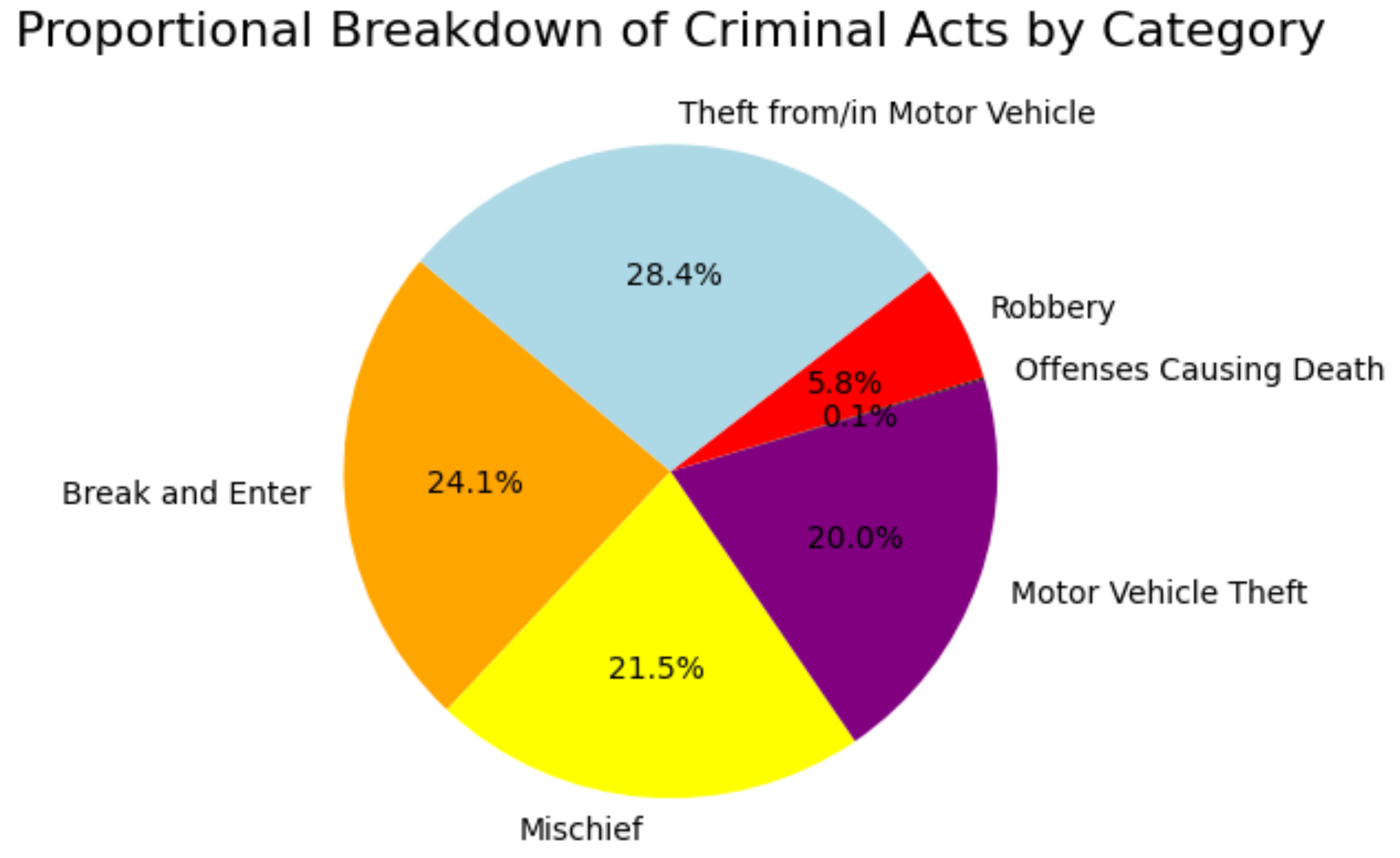
Figure 2.
Feature Importance using the Chi-square Statistical Method.
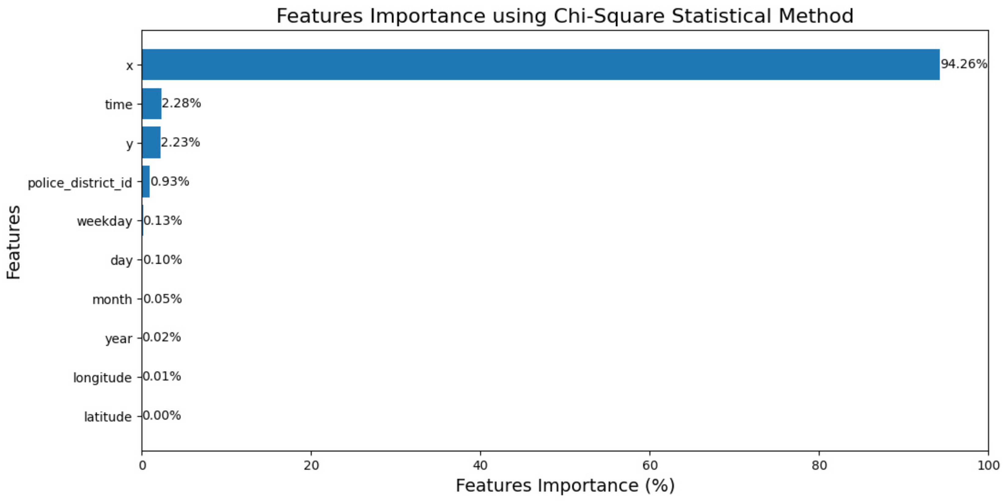
Figure 3.
Distribution of Crime Categories over Different Times of the Day.
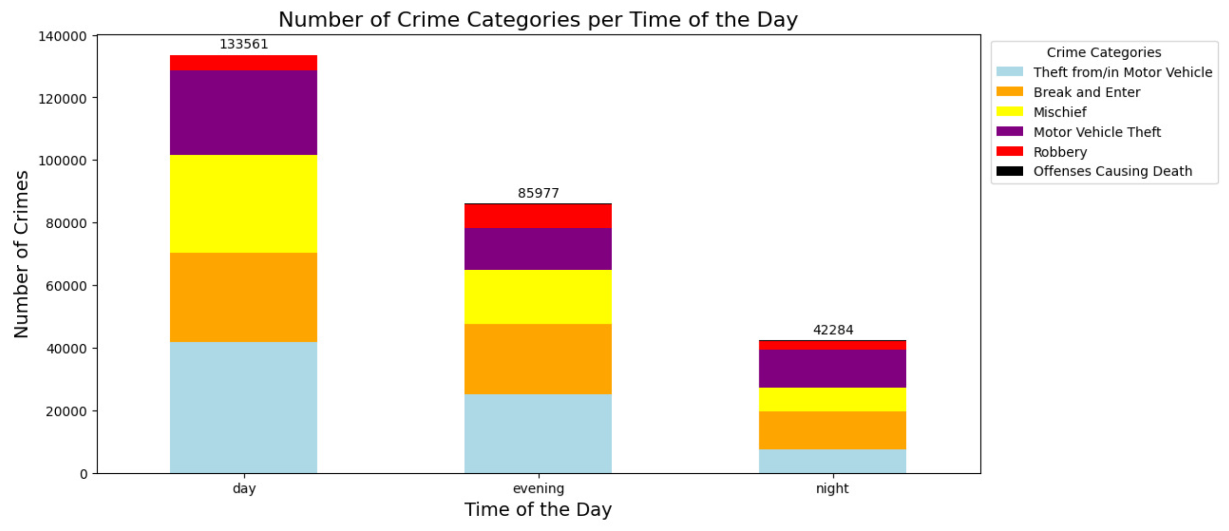
Figure 4.
Weekly Distribution of Crime Categories.
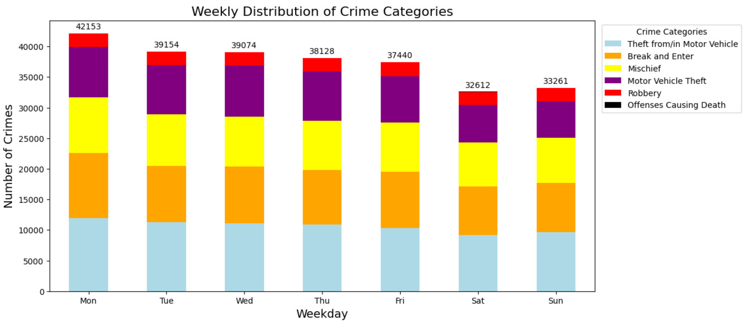
Figure 5.
Monthly Distribution of Crime Categories.
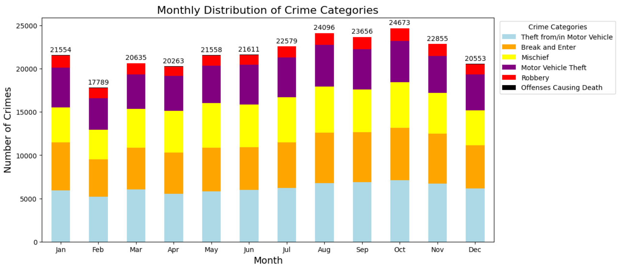
Figure 6.
Yearly Distribution of Crime Categories.
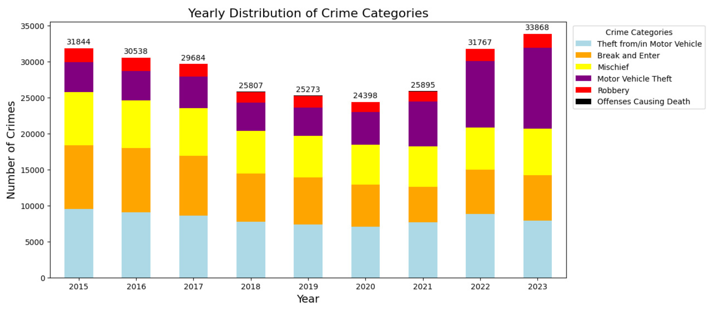
Figure 7.
Heatmap of Crime Numbers by Time of Day and Day of the Week.
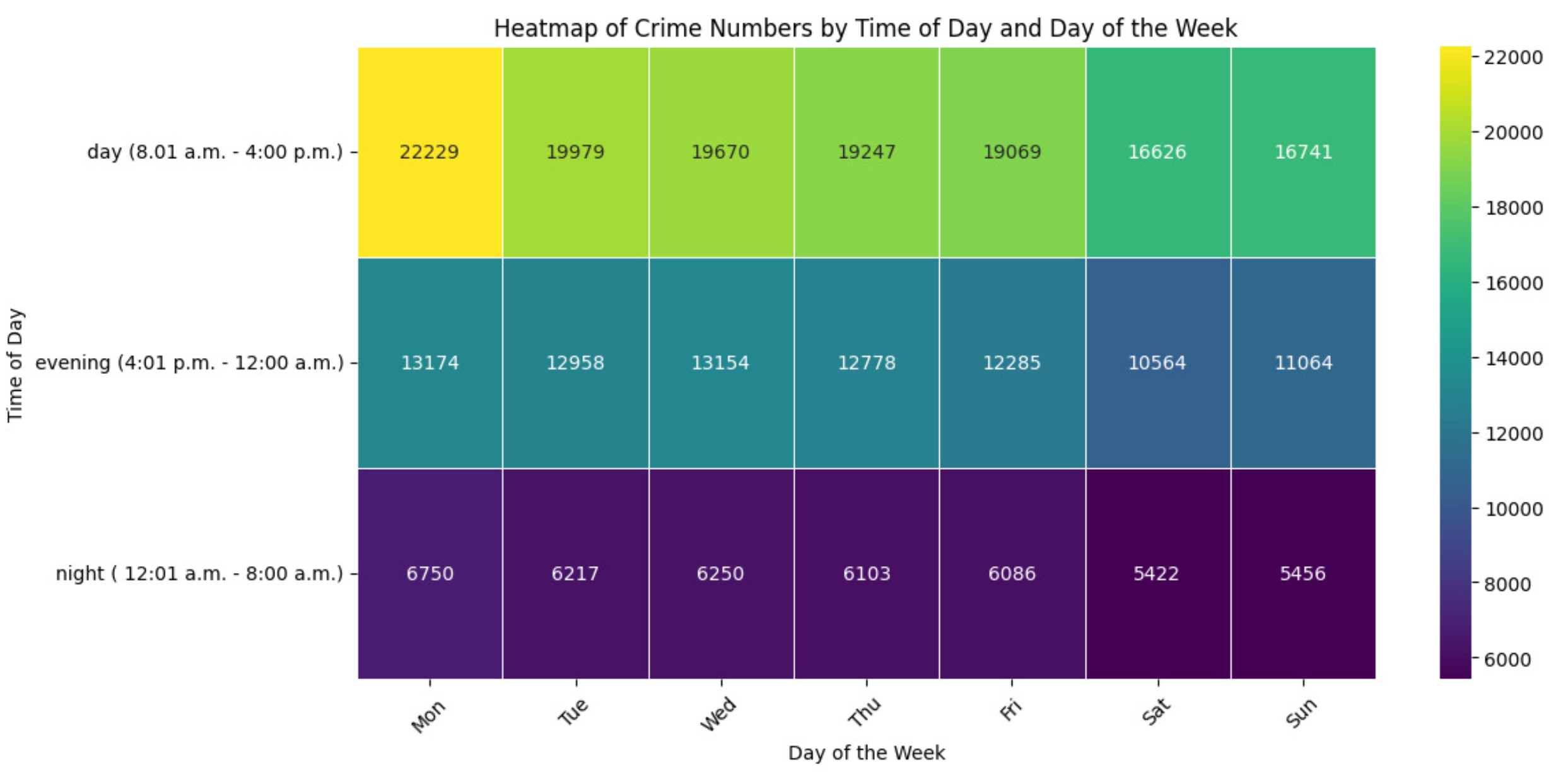
Figure 8.
XGBoost Model Confusion Matrix.
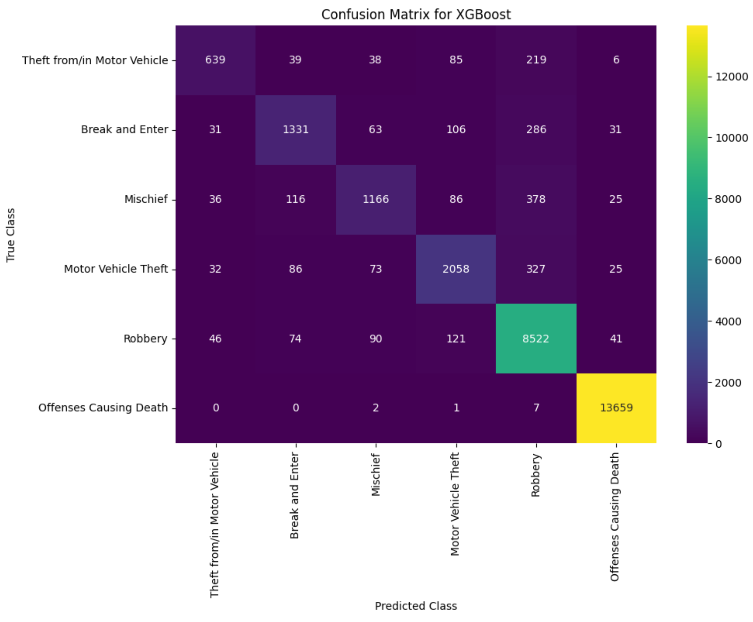
Figure 9.
Decision Tree Model Confusion Matrix.
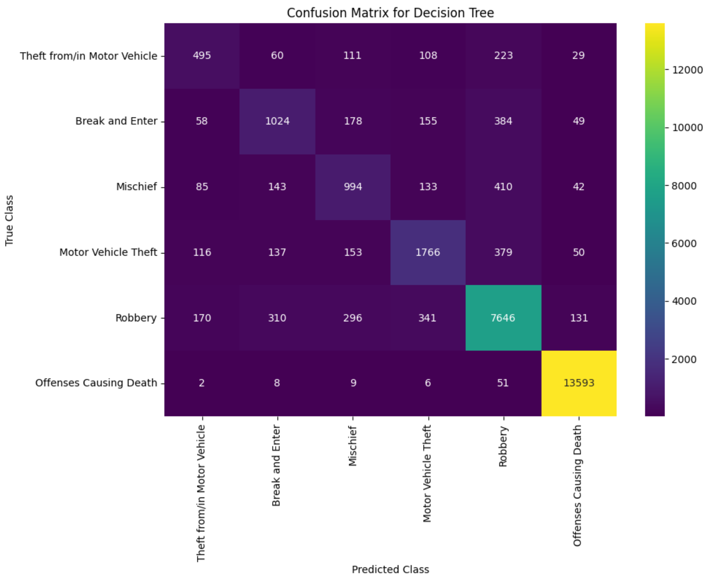
Figure 10.
Random Forest Model Confusion Matrix.
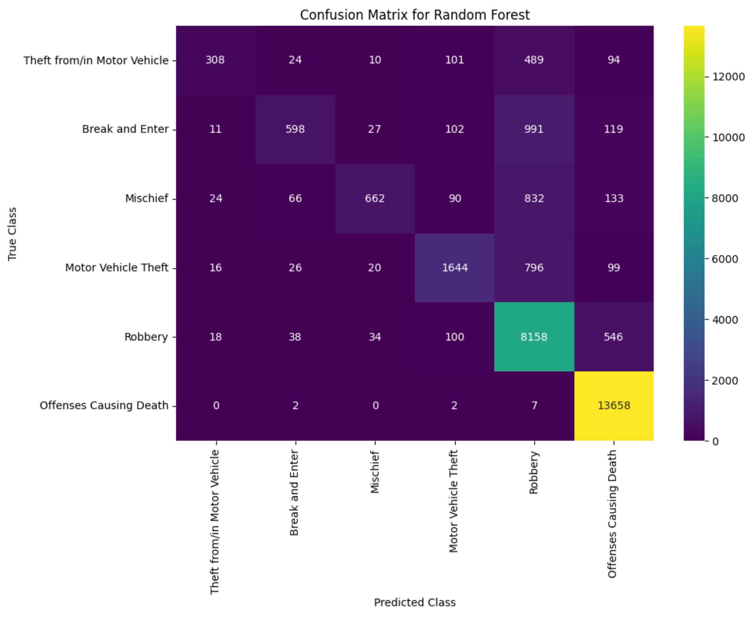
Figure 11.
Archictecture of the web application.
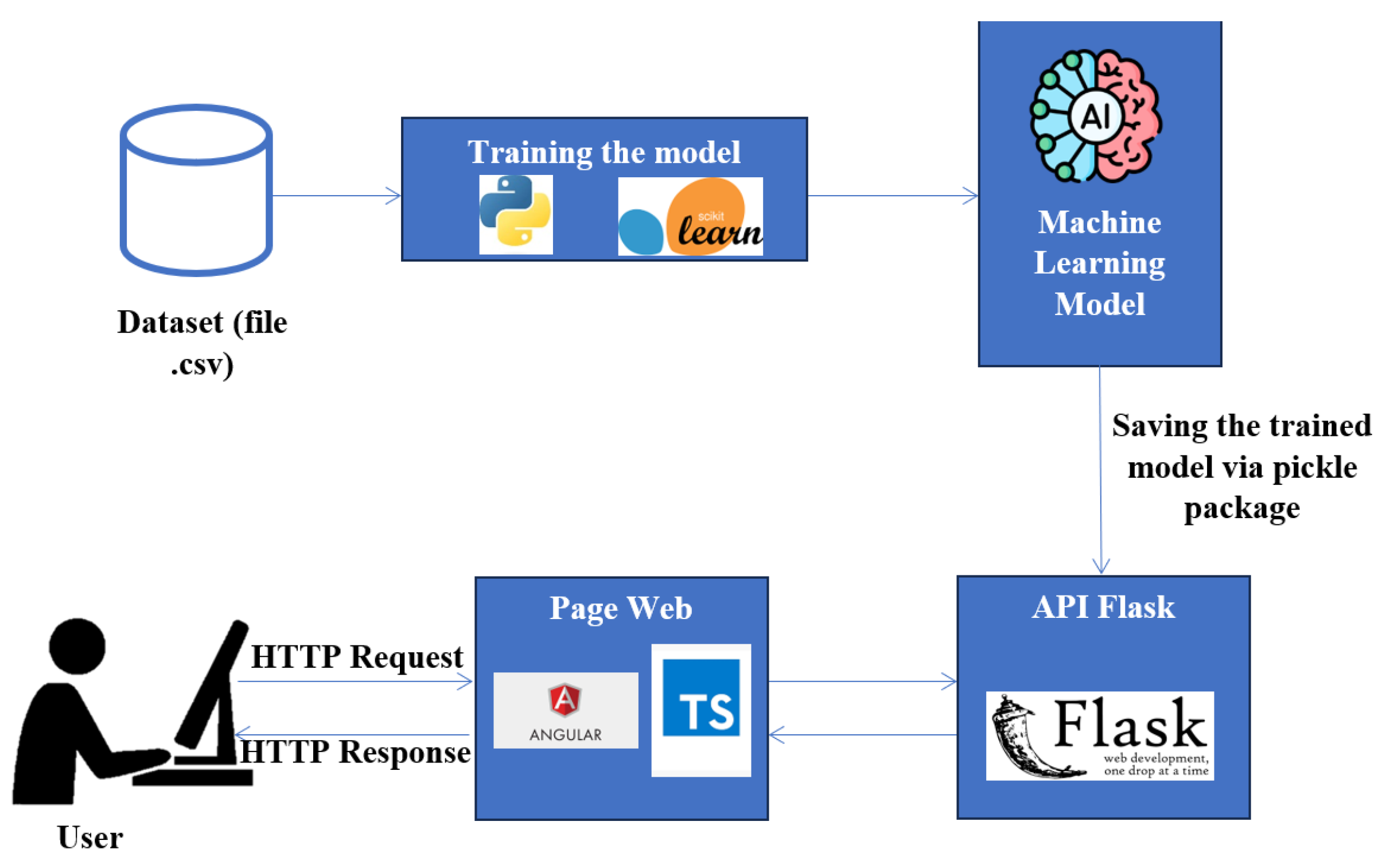

Table 1.
Comparative analysis of machine learning approaches to crime category prediction.
| Study | Focus | Data Used | Models Evaluated | Key Findings |
|---|---|---|---|---|
| [5] | Crime category prediction | Crime and Communities dataset, UCI | RF, SVM | RF outperforms SVM with 99% accuracy. |
| [6] | Crime category prediction in Chicago | Chicago crime data | Decision Trees, Naive Bayes | Decision Trees outperform Naive Bayes with 91.68% accuracy. |
| [7] | Crime prediction in India | NCRB Indian criminal records | SVM, J48, SMO, Naïve Bayes, Bagging, Random Forest | Ensemble method (SBCPM) shows superior performance with 99.5% accuracy. |
| [8] | Crime prediction in Dubai | Dubai crime data | Random Forest, KNN, SVM, ANN, Naïve Bayes, Decision Tree | KNN outperforms others with 78.47% accuracy. |
| [9] | Crime prediction in urban areas | Chicago Police Department’s CLEAR system data | Random Forest, KNN, AdaBoost, Neural Networks | Neural Network shows highest accuracy at 90.77%. |
| [10] | Automated crime report analysis | San Francisco Crime dataset | Random Forest | Achieved 86.5% accuracy, precision, recall, F-score, AUC of 0.98. |
| [11] | Criminal activity prediction in San Francisco | San Francisco criminal incidents data | Decision Tree, KNN, Random Forest, AdaBoost | Random Forest with random undersampling achieved 99.16% accuracy. |
| [12] | Crime trend analysis in Bangladesh | Bangladesh crime data | KNN, Naive Bayes, Linear Regression | KNN outperforms with 76.92% accuracy in predicting safe routes. |
| [13] | Crime data prediction | Chicago and Los Angeles crime data | LSTM, ARIMA, Logistic Regression, SVM, Naive Bayes, KNN, Decision Tree, MLP, Random Forest, XGBoost | LSTM effective in time series forecasting; ARIMA predicts crime trends. |
| [14] | Crime prediction with machine learning | San Francisco crime data | Naive Bayes, Random Forest, Gradient Boosting Decision Trees | Gradient Boosting Decision Trees show superior performance with 98.5% accuracy. |
| Current Work | Crime category prediction in Montreal | Montreal crime data (2015-2023) | XGBoost, Decision Trees, Random Forest | XGBoost outperforms others with superior precision, accuracy, recall, and F1 score. Deployed as a web application. |
Table 2.
Description of dataset attributes.
| Attribute | Description |
|---|---|
| Crime category | The nature of the event:
|
| Date | Date of event report to MCPS in YYYY-MM-DD format. |
| Time of Day | Time of day the event was reported to MCPS:
|
| Police District Number | Police district number for the neighborhood where the incident occurred. |
| X | Geospatial position according to the MTM8 projection (SRID 2950). |
| Y | Geospatial position according to the MTM8 projection (SRID 2950). |
| Latitude | Geographical position of the event at an intersection according to the WGS84 geodetic reference system. |
| Longitude | Geographical position of the event at an intersection according to the WGS84 geodetic reference system. |
Table 3.
Summary of Missing Data by Attribute.
| Attribute | Number of Missing Data | Percentage Missing (%) |
|---|---|---|
| X | 47193 | 16.854 |
| Y | 47193 | 16.854 |
| Longitude | 47193 | 16.854 |
| Latitude | 47193 | 16.854 |
| Police District Number | 5 | 0.0018 |
Table 4.
Manual Encoding for the Categorical Variable Crime Category.
| Crime Category | Numeric Encoding |
|---|---|
| Theft from/in Motor Vehicle | 0 |
| Break and Enter | 1 |
| Mischief | 2 |
| Motor Vehicle Theft | 3 |
| Robbery | 4 |
| Offenses Causing Death | 5 |
Table 5.
Manual Encoding for the Categorical Variable Time.
| Time | Numeric Encoding |
|---|---|
| Day | 0 |
| Evening | 1 |
| Night | 2 |
Table 6.
Performance of Data Balancing Algorithms.
| Balancing Algorithm | Accuracy |
|---|---|
| SMOTE | 0.588510 |
| SMOTE-Tomek | 0.474414 |
| SMOTE-ENN | 0.632867 |
| ADASYN | 0.902227 |
Table 7.
Summary of the Classification Report.
| Class | Precision | Recall | F1-score | Support | Accuracy |
|---|---|---|---|---|---|
| Results for XGBoost | |||||
| Theft from/in Motor Vehicle | 0.82 | 0.62 | 0.71 | 1026 | |
| Break and Enter | 0.81 | 0.72 | 0.76 | 1848 | |
| Mischief | 0.81 | 0.65 | 0.72 | 1807 | |
| Motor Vehicle Theft | 0.84 | 0.79 | 0.81 | 2601 | |
| Robbery | 0.88 | 0.96 | 0.91 | 8894 | |
| Offenses Causing Death | 0.99 | 1.00 | 0.99 | 13669 | |
| Weighted Avg | 0.91 | 0.92 | 0.91 | 29845 | 0.92 |
| Results for Decision Tree | |||||
| Theft from/in Motor Vehicle | 0.53 | 0.48 | 0.51 | 1026 | |
| Break and Enter | 0.61 | 0.55 | 0.58 | 1848 | |
| Mischief | 0.57 | 0.55 | 0.56 | 1807 | |
| Motor Vehicle Theft | 0.70 | 0.68 | 0.69 | 2601 | |
| Robbery | 0.84 | 0.86 | 0.85 | 8894 | |
| Offenses Causing Death | 0.98 | 0.99 | 0.99 | 13669 | |
| Weighted Avg | 0.85 | 0.86 | 0.85 | 29845 | 0.86 |
| Results for RF | |||||
| Theft from/in Motor Vehicle | 0.82 | 0.30 | 0.44 | 1026 | |
| Break and Enter | 0.79 | 0.32 | 0.46 | 1848 | |
| Mischief | 0.88 | 0.37 | 0.52 | 1807 | |
| Motor Vehicle Theft | 0.81 | 0.63 | 0.71 | 2601 | |
| Robbery | 0.72 | 0.92 | 0.81 | 8894 | |
| Offenses Causing Death | 0.93 | 1.00 | 0.96 | 13669 | |
| Weighted Avg | 0.84 | 0.84 | 0.82 | 29845 | 0.84 |
Disclaimer/Publisher’s Note: The statements, opinions and data contained in all publications are solely those of the individual author(s) and contributor(s) and not of MDPI and/or the editor(s). MDPI and/or the editor(s) disclaim responsibility for any injury to people or property resulting from any ideas, methods, instructions or products referred to in the content. |
© 2024 by the authors. Licensee MDPI, Basel, Switzerland. This article is an open access article distributed under the terms and conditions of the Creative Commons Attribution (CC BY) license (http://creativecommons.org/licenses/by/4.0/).
Copyright: This open access article is published under a Creative Commons CC BY 4.0 license, which permit the free download, distribution, and reuse, provided that the author and preprint are cited in any reuse.


