Submitted:
18 June 2024
Posted:
18 June 2024
Read the latest preprint version here
Abstract
Recent measurements in the MRX laboratory plasma [J.Yoo et al, Phys. Rev. Lett. 132, 145101 (2024)] have evidenced the role of lower hybrid drift waves produced during magnetic reconnections in producing an effective anomalous resistivity and heating of electrons. A detailed modelization of the energy transfer from the waves to electrons is missing, though. In this work, we attempt such an exercise using a Hamiltonian test-particle model for wave-electron interaction, valid for low-β weakly collisional plasmas. Quantitative agreement with MRX results is found.
Keywords:
Magnetic reconnection
; Lower Hybrid drift waves
; electron-wave interaction
; Hamiltonian model
; laboratory plasmas
; MRX device
; non-adiabatic dynamics
1. Introduction
Reconnections are ubiquitous processes in magnetized plasmas: laboratory, stellar, and planetary ones [1]. They involve sudden changes in the topology of the magnetic field, that rearranges into a state of lower energy. Part of the initial free energy is traveled away from the reconnection region by waves, or converted into kinetic energy of ions and electrons. Reconnection is a complex process, which defies a unique description, since is heavily dependent upon the geometry of the magnetic field and the physical conditions existing; it is therefore a topic still actively studied [2]. During reconnection, a lot of electromagnetic activity is produced, in the form of broadband turbulence or coherent waves, which can interact with the ions and/or the electrons, delivering energy to the kinetic component of the plasma. A topic of current investigation concerns the mechanisms that allow energy to flow between waves and particles.
The Magnetic Reconnection eXperiment (MRX) is a device to study the fundamental physics issues of magnetic reconnection in a well-controlled laboratory environment [3]. A recent paper by Yoo et al [4] reports the results of a campaign of detailed measurements of fields and particles performed at MRX. Besides a full 2D probe array for magnetic field reconstruction, an electrostatic probe was employed, inserted at the reconnection region, allowing fast measurements of electron density, temperature, and electric field. These measurements allowed (I) to establish the existence of fluctuations of the electric signal that, by means of a theoretical model, were identified as electrostatic Lower Hybrid (LH) drift waves propagating almost perpendicularly to the magnetic field. (ii) Established the existence of fluctuations in the electron density, quite well correlated with the LH waves. These waves affect differently ions and electrons, producing an effective collisionless relative drag, and thus an anomalous contribution to resistivity (see Mozer et al [5]). (iii) Accordingly, ohmic dissipation increases; a positive correlation was observed between the electron temperature and the amplitude of the electric fluctuations.
These observations allow to establish for the first time in a laboratory device the role of electrostatic LH waves in driving current and in heating the plasma. Some gaps are still to be filled, though. The precise mechanism through which LH waves deliver energy to the electrons is not yet understood. Collisionless Landau damping appears problematic as a heating mechanism, since it requires a finite parallel wavenumber for the resonance condition to be fulfilled, whereas MRX experiments show that the modes with the highest linear growth rate, that constitute most of the power spectrum, have .
In this work, we propose that electron heating may occur via energization of the perpendicular degrees of freedom, rather than the parallel one, through the interaction with low-frequency high-amplitude electromagnetic waves. This mechanism has frequently been invoked in astrophysical literature, often as a candidate for ion heating by Alfvèn waves, but its range of application is more widespread. Incidentally, the first papers introducing it were in connection precisely with a problem of particle heating by LH waves [6,7,8,9,10,11,12,13,14,15,16,17,18,19]. We sketch a Hamiltonian model of LH wave-particle interaction in the presence of a strong guide magnetic field, in a simplified geometry, representative of MRX conditions. We will show that, when feeding the model with MRX plasma parameters, we will be able to recover quantitatively the measured amount of heating, in terms of temperature gain per electron.
We justify our test-particle approach on the basis of the fact that MRX plasmas are low- and just weakly collisional. We cannot model the anomalous resistivity since it relies upon the self-consistent differential motion of ions and electrons but, as an interesting corollary, we will show that wave-particle correlations along the parallel direction, reminiscent of the collisionless Landau damping mechanism, arise spontaneously within our framework.
2. Methods
We will restrict ourselves to the reconnection region, where the reconnecting component of the magnetic field, aligned along the y-axis, is small and will be neglected in comparison to the perpendicular guide field , assumed constant and aligned along the z axis. Written in terms of the vector potential, the magnetic field is
We add, then, a monochromatic wave propagating perpendicularly to the magnetic field:
The wave has both magnetic and electric components:
In particular, the oscillating electric field is oriented along the out-of-reconnection plane direction and parallel to the guide field, like in the experiment. According to Yoo et al, the spectrum of LH fluctuations is almost monochromatic except at the largest amplitudes, hence retaining just a single wave does not like a poor approximation.
In MRX, fluctuations superimpose upon a mean flow along z, driven by an average electric field and braked by collisions. Here, we place ourselves in a reference frame moving with the mean flow, thus treating electrons as initially at rest along the z-axis, and neglect both collisions and the macroscopic electric field.
In the following lines, for convenience, we will be using dimensionless quantities: time is given in units of , with the Larmor angular frequency. Lengths are normalized to the thermal Larmor radius , where is the measured electron plasma temperature and are the electron charge and mass. The single-particle Hamiltonian is
Since H does not depend upon the coordinates , the momenta are constant of the motion and have been dropped in the last line, alongside a constant term. Had we accounted for the reconnecting component of the magnetic field, the system would have been fully three-dimensional.
Hamiltonian (4), through the rescaling and , may be mapped into the paradigmatic form
Since features an explicit time dependence that is slow compared to the cyclotron motion, one might näively expect that the corresponding dynamics be always adiabatic and reversible. The literature cited above showed, instead, that this is true only for small wave amplitudes; there is a transition from adiabatic to non-adiabatic dynamics in correspondence of a trespassing the threshold . This condition corresponds to the appearance of a slow (moving with the wave frequency) separatrix in the particle phase space. In the static case, the separatrix divides orbits into totally disjointed basins while, in the dynamical regime, it is permeable. However, close to the separatrix, the period of the orbit becomes very large, exceeding the wave period. Thus, the adiabaticity hypothesis, which relies upon the particle orbit period being much smaller than the wave period, breaks down, any crossing of the separatrix is an essentially irreversible process, and net energy transfer between particle and wave may take place 1.
The threshold amplitude writes . The amplitude of the electric field associated to the wave is , hence the threshold condition can be written as . In physical units, it becomes
where is the thermal speed. The average energy gained per particle in the non-adiabatic regime is a question that, quantitatively, has not yet received a full investigation. Some partial investigations are reported in [15], but only cold particles were there considered, i.e., their initial distribution was practically mono-energetic, close to zero. In this paper, we are going to repeat the exercise using a realistic thermal initial distribution.
Hamilton equations from Eq. (4) were integrated in time using one symplectic algorithm built into Mathematica software, and another one implemented from ref. [21]. Here below we provide the results of a scan done varying the wave amplitude . The numerical strategy is the same employed elsewhere: we switch on and off the wave through a shape function , with
By comparing the particle energy prior to and after the switching of the wave, we get the amount of heating. For each value of A, 2400 independent trajectories were evolved. Initial conditions were randomly sampled from a thermal distribution, i.e., and r picked up respectively from a zero-mean, unit-variance normal distribution, and from the uniform distribution in , and . All parameters were taken from MRX measurements. Using non-normalized quantities: Gauss, eV, , MHz. The shape function grows up and falls down over the MRX reconnection time scales: .
3. Results
The main result of this work is summarized in Figure 1. The threshold amplitude of Eq. (6) corresponds to 85 V/m for the parameters employed. There is energy gain by the electrons only beyond this threshold: compare the two leftmost points with the others. The figure should be compared with Figure 4 of the paper [4], in particular with the red dots, which correspond to the case of the largest guide field, closest to the geometry employed in the present work: there, the electron temperature rises from slightly more than 7 eV to about 10 eV over the range 50-150 V/m, nicely consistent with our result.
Figure 2 shows a sample of the time trace for one energized trajectory, alongside the time trace of f employed in these simulations, to give an insight about the typical dynamics experienced by electrons during their interaction with the wave. In particular, we point the attention to the wild energy fluctuations which during the time interval in the figure. They greatly exceed the final stationary energy of the particle, but only transiently: as long as the wave amplitude does not exceed the required threshold, ultimately the electron lands back to its initial energy once the wave has disappeared.
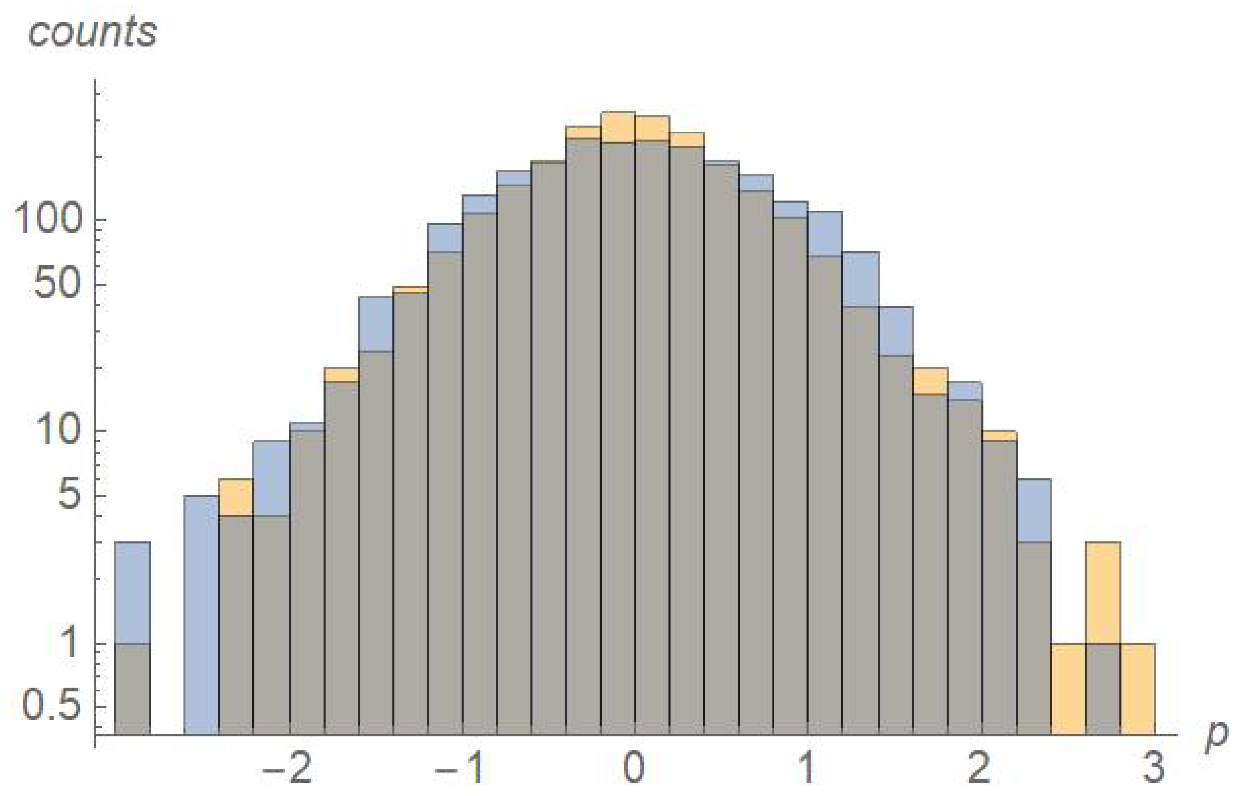
In the Figure 3 we show the histograms of the initial and final particle momenta for the case with V/m. It is interesting that the final distribution remains fairly close to a thermal (normal) curve. This result was not granted from earlier studies using monoenergetic initial distributions, and is comforting since experimental measurements hint to a true heating, not just electron energization.
We remark that, even though the wave electric field is parallel to the guide magnetic field, energization of the electrons occurs along the x direction, perpendicular to . Since Hamilton’s equation for the motion along the magnetic field writes (setting ), when the wave vanishes () we are sure that the particle stops moving along z: no energy is acquired along the parallel direction.
Our simulations do not involve interactions between particles–and in particular between ions and electrons–therefore the subject of the anomalous resistivity is outside the scope of this work. Yet, the analysis of the particle dynamics reveals interesting aspects. n Figure 4 we plot one time trace of the quantity , where is the computed trajectory. The plot refers to the flat-top phase, where . Although the plot refers to just one case, the inspection of several trajectories shows that the picture is totally generic: the particle trajectory exhibits a quasi-periodic trend, with intervals where it slowly drifts around two attractors, placed at the phase , interrupted by sudden jumps from the one to the other.
Figure 4.
Time trace of for one trajectory. Here, V/m, .
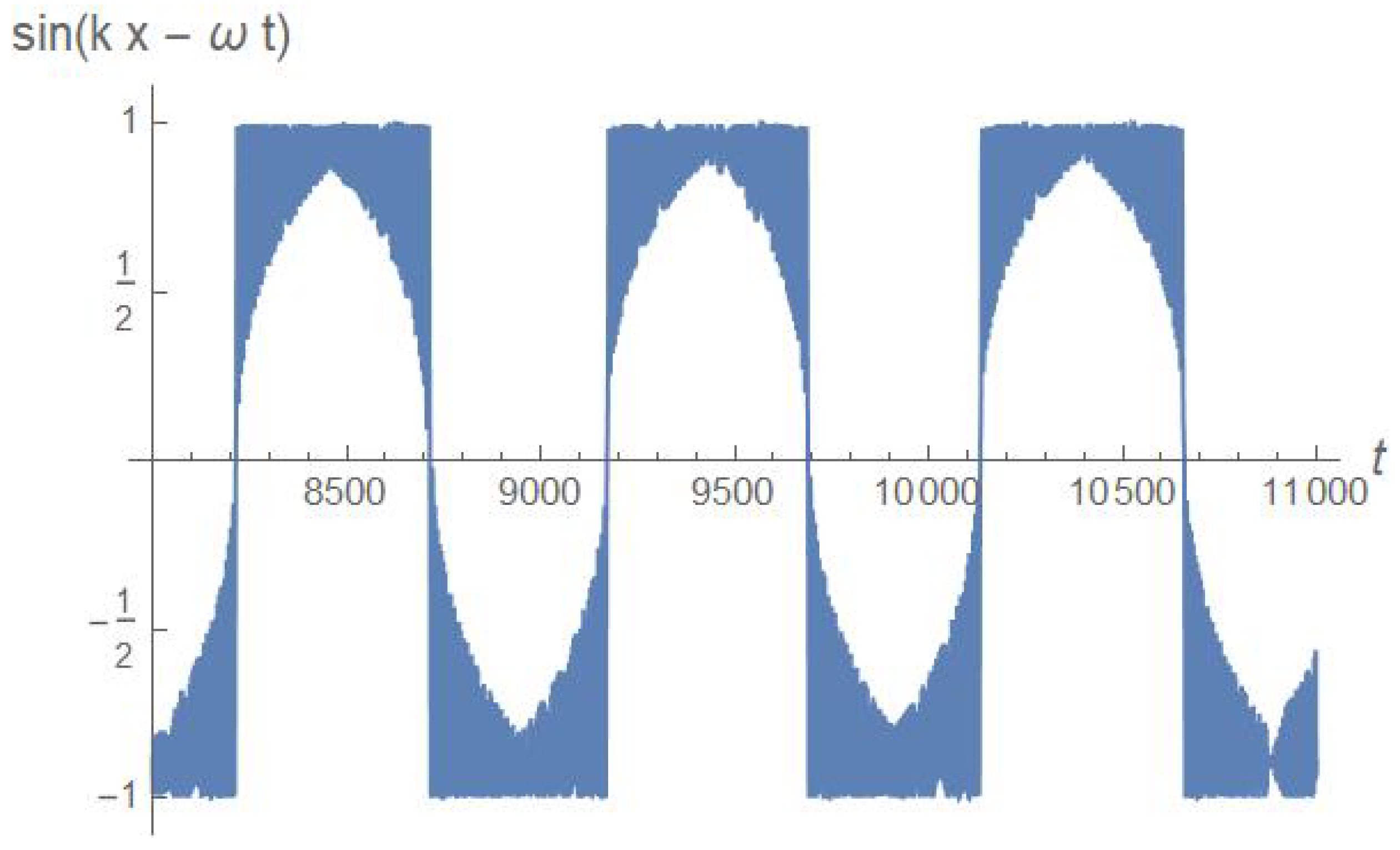
From Eq. (4) we retrieve the equation of motion along z:
where we have set , consistently with our choice of initial conditions. After another derivative we get Newton’s law
The dynamics of Figure 4 consists of finite intervals where the particle stays almost in phase with the peaks of the electric field: (), which is a feature of the Landau damping. This condition, which corresponds to the state of maximal acceleration by the electric field, is unstable since is incompatible over long times with the condition from Eq. 8, thus the system jumps repeatedly between the two fixed points. Yoo et al introduce the anomalous drag term which quantifies the correlation between the particle and the electric field oscillations and the contribution to the resistivity by the fluctuating terms. Within our framework, the analog of D, normalized to the electric field amplitude, is
where is the particle trajectory, and the average is performed both over time and over all the trajectories.
In our case there is no symmetry-breaking term, correlated and anti-correlated phases are equally likely, thus vanishes. However, we may speculate about what would happen if an efficient symmetry-breaking mechanism, that allows only correlated (or anti-correlated) phases to survive, were added. If we average over just the time windows where it is positive, we get , which compares fairly well with the figure coming from the measurements of Yoo et al. By comparison, a perfectly sinusoidal trend would yield . All this is highly speculative, yet it is suggestive that the observed correlation might arise as a consequence of this kind of resonance.
Funding
This research received no external funding
Data Availability Statement
The source code and the datasets are available from the author upon request.
Acknowledgments
Discussions with D. Bonfiglio, S. Cappello, D.F. Escande, M. Gobbin are gratefully acknowledged
Conflicts of Interest
The author declares no conflicts of interest.
References
- M. Yamada, R. Kulsrud, and H. Ji, Rev. Mod. Phys. 2010; 82, 603.
- H. Ji, W. Daughton, J. Jara-Almonte, A. Stanier, and J. Yoo, Nat. Rev. Phys. 2022; 4, 263.
- M.Yamada et al. Phys. Plasmas, 1997; 4, 1936.
- J. Yoo, et al, Phys. Rev. Lett. 2024; 132, 145101.
- F.S. Mozer, M. Wiber, and J.F. Drake, Phys. Plasmas. 2011; 18, 102902.
- C.F.F. Karney, Phys. Fluids. 1979; 22, 2188.
- J.F. Drake and T.T. Lee, Phys. Fluids. 1981; 24, 1115.
- J.M. McChesney, R.A. Stern and P.M. Bellan, Phys. Rev. Lett. 1987; 59, 1436.
- L. Chen, Z.Lin, R. White, Phys. Plasmas. 2001; 8, 4713.
- O. Ya. Kolesnychenko, V.V. Lutsenko, R.B. White, Phys. Plasmas. 2005; 12, 102101.
- C.B.Wang, C.Wu and P.H.Yoon, Phys. Rev. Lett. 2006; 96, 125001.
- X. Li, Q. Lu, B. Li, Ap J. 2007; 661, L105.
- Z. Guo, C. Crabtree, L. Chen, Phys. Plasmas. 2008; 15, 032311.
- B.D.G.Chandran, B. B.D.G.Chandran, B.Li, B.N. Rogers, E. Quataert, and K.Germaschewski, Ap.J. 2010; 720, 503. [Google Scholar]
- D.F. Escande, V. Gondret, F. Sattin, Sci. Rep. 2019; 9, 14274.
- K.Stasiewicz. MNRAS, 2020; 496, L133.
- K.Stasiewicz and B. Eliasson, Ap. J. 2020; 904, 173.
- Y. Dae Yoon and P.M.Bellan, Phys. Plasmas. 2021; 28, 022113.
- S.S.Cerri, L.Arzamasskiy, and M.W.Kunz, Ap.J. 2021; 916, 120.
- F. Sattin, D.F. Escande, Phys. Rev. E. 2023; 107, 065201.
- R.I. McLachlan and P. Atela. Nonlinearity, 1992; 5, 541.
| 1 | The threshold condition places a constraint upon the wave amplitude which is often difficult to satisfy in laboratory (and sometimes also astrophysical) plasmas, where fluctuations are ordinarily small with respect to mean fields. Although it is not relevant to the present work, we mention that recently we showed that this threshold is not always needed, since under some conditions it can be traded for a threshold upon the duration of the wave-particle interaction, in a way reminiscent of quantum-mechanics indeterminacy relations: see the paper [20] |
Figure 1.
Final temperature (average energy of the test particle) when the initial temperature eV versus the amplitude of the wave electric field. The threshold value (Eq. 6) is V/m, corresponding to the second point from the left.
Figure 1.
Final temperature (average energy of the test particle) when the initial temperature eV versus the amplitude of the wave electric field. The threshold value (Eq. 6) is V/m, corresponding to the second point from the left.
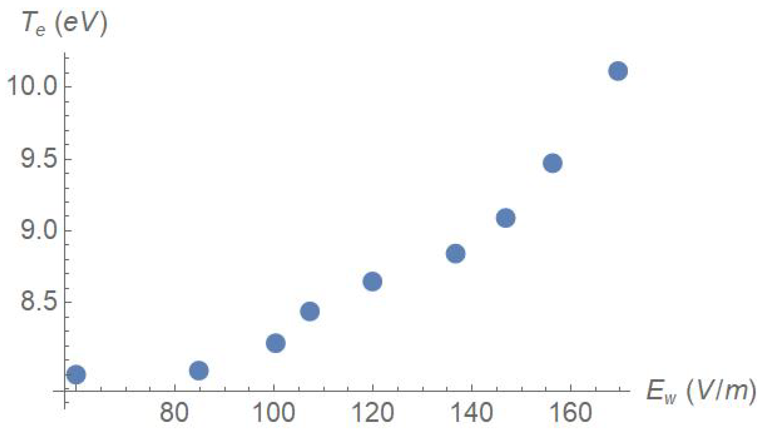
Figure 2.
An example of time trace of one simulation. The blue curve is the kinetic energy , the yellow curve is . This run features V/m: twice the threshold for the onset of nonadiabatic motion, and an initially almost static particle:
Figure 2.
An example of time trace of one simulation. The blue curve is the kinetic energy , the yellow curve is . This run features V/m: twice the threshold for the onset of nonadiabatic motion, and an initially almost static particle:
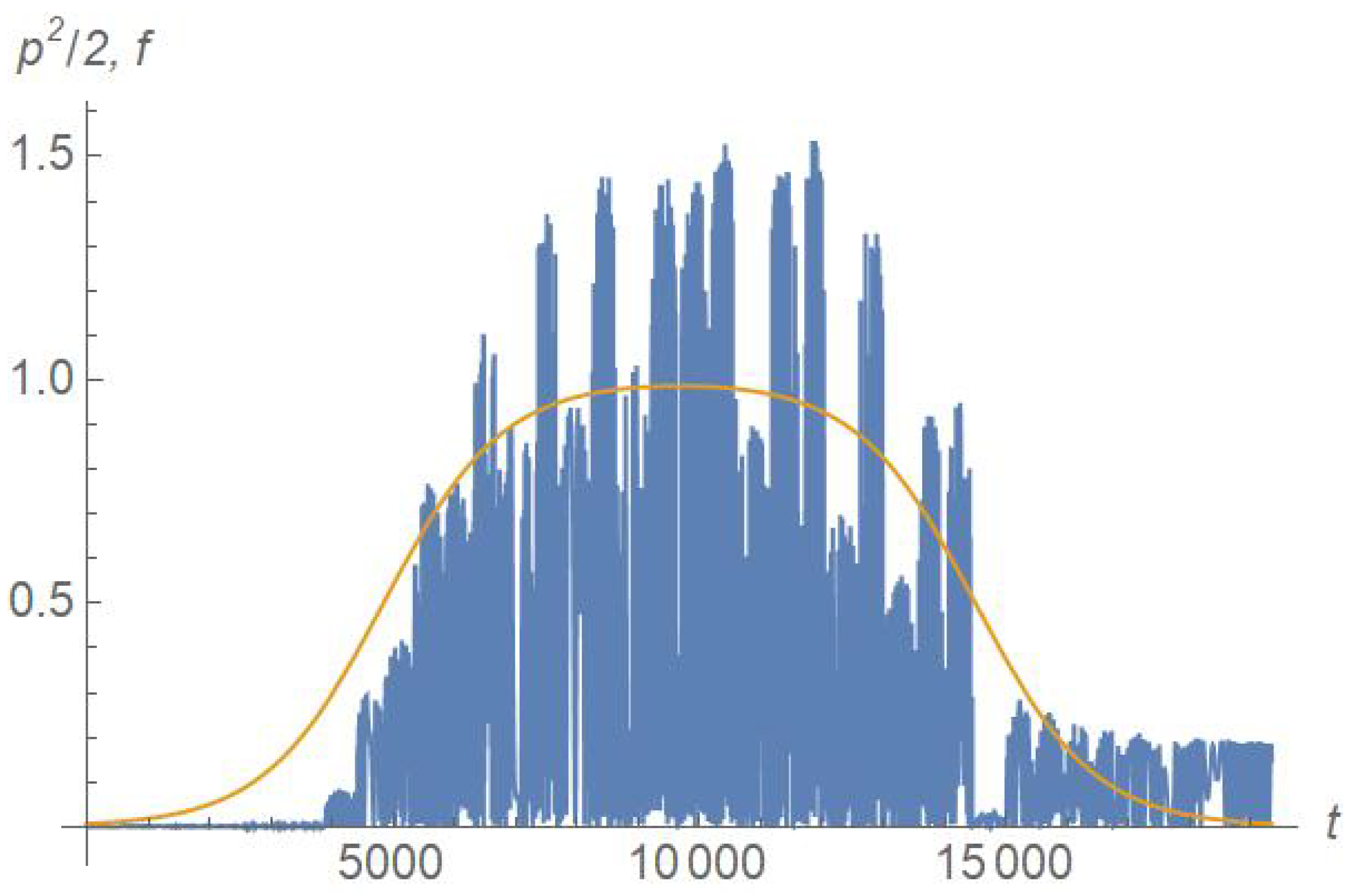
Figure 3.
Histograms of the initial (yellow) and final (blue) momentum distribution for the case with V/m.
Figure 3.
Histograms of the initial (yellow) and final (blue) momentum distribution for the case with V/m.
Disclaimer/Publisher’s Note: The statements, opinions and data contained in all publications are solely those of the individual author(s) and contributor(s) and not of MDPI and/or the editor(s). MDPI and/or the editor(s) disclaim responsibility for any injury to people or property resulting from any ideas, methods, instructions or products referred to in the content. |
© 2024 by the authors. Licensee MDPI, Basel, Switzerland. This article is an open access article distributed under the terms and conditions of the Creative Commons Attribution (CC BY) license (http://creativecommons.org/licenses/by/4.0/).
Copyright: This open access article is published under a Creative Commons CC BY 4.0 license, which permit the free download, distribution, and reuse, provided that the author and preprint are cited in any reuse.


