
Submitted:
10 June 2024
Posted:
13 June 2024
You are already at the latest version
Abstract
Input reconstruction problem is usually encountered in the areas such as virtual sensing, image restoration, sensor linearization, and communications. The input reconstruction problem can be seen as an inverse problem. Given a nominal system, two types of approaches are commonly used for solving the inverse problem. The first one is to directly invert the nominal system, and the second one is to derive an inversion of the nominal system in an indirect way. However, for the first type of approaches, system inversion cannot be directly conducted under some conditions such as there exist nonminimum-phase zeros in the nominal system, while for the second type of approaches, simultaneously guaranteeing stability and causality of the obtained inversion is still not solved well. In order to avoid the drawbacks existing in the two types of approaches, an alternative approach is proposed for input reconstruction. In this approach, the input signal is first modeled as the output of a state-space model, afterwards two Kalman filters for the model resulted by combining the input signal model and the nominal system model are implemented alternatively such that the input signal can be sequentially reconstructed in an infinite horizon. The proposed input reconstruction approach is applied in two examples, and simulation results can illustrate the effectiveness of the proposed approach.
Keywords:
Kalman filtering
; Input reconstruction
; Inverse modeling
; Inverse problems
; Virtual sensing
1. Introduction
Inverse problems are important problems in both science and engineering [1,2], such as virtual sensing [3], image processing (e.g., image restoration [4]), sensor linearization [5], and digital predistortion for radio frequency communications [5]. In the point of view of system identification, there are two kinds of inverse problems [6]:
- (i)
- Reconstruct the system inputs based on the system outputs and the inverse system model, which is also called the input reconstruction problem or the inverse system identification problem, see Figure 1(a).
- (ii)
- Identify the forward system model based on the input-output data, which is a normal system identification problem, see Figure 1(b).
In this paper, the first type of inverse problems (i.e., the input reconstruction problem) is investigated. Generally, there are two types of approaches for solving the first kind of inverse problems:
- (i)
- The first approach is to make a direct inversion of the nominal system firstly, and then input reconstruction can be conducted. Denote the transfer function of a discrete-time model as of which a state-space realization is , when the inverse of the feedthrough term does not exist, the direct inversion of the model cannot be conducted [7,8]. In addition, if there exist nonminimum-phase zeros in , an unstable inversion solution will be obtained [9]. So in practical applications of direct inversion approaches,
- (ii)
-
The second approach is to obtain an inverse system model of the nominal system model indirectly, and input reconstruction can then be realized. However, in order to obtain a stable inversion, there are a number of drawbacks in existing approaches:
- (a)
- (b)
- (c)
- (d)
- (e)
As seen, for some indirect system inversion approaches, even though a stale inversion can be obtained, an infinite or a finite pre-actuation is still needed, which cannot be applied well in practice because sometimes the desired output in unknown. In order to solve the input reconstruction problem in a better way, in this paper an alternative approach is proposed. The presented approach can guarantee the stability of the input reconstructor, and simultaneously the proposed approach does not need any pre-actuation; Moreover, the approach can be applied to stable or unstable, proper or improper systems1 with input to be reconstructed, and there is also no requirement for the type of input and output signals; Furthermore, it does not suffer non-convex or input noise problems.
The remainder of the paper is organized as follows. In Section 2, the modeling of signals with finite-length is introduced, based on which in Section 3 an alternative recursive Kalman filter-based input reconstruction approach is proposed. In Section 4, the performance of the proposed approach is verified and analyzed, and finally conclusions and future perspectives are given in Section 5.
2. Limited-Length Signal Modeling
In this section, the modeling of limited-length signals is illustrated. With the idea of Limited-length signal modeling, an alternative input reconstruction approach is proposed in Section 3.
Given a discrete-time signal with length N and the sampling period in seconds, now assume that the limited-length signal is a whole period of a periodic signal , so within the length N, the signal can be represented as the output of the following state-space model [24], i.e.,
where denotes the state vector, the term denotes the modeling error which is induced by the limited dimension of the matrix , and the matrices and can be represented as
and
respectively, where denotes a zero vector or a zero matrix, and the individual block entries in these block matrices are
and
where , for .
In the end of this section, the following assumption is made.
Assumption A1.
The sequence is assumed to be a white-noise sequence. The covariance function of the white-noise sequence is where is a positive and constant scalar value, and is the Kronecker Delta function depending on two integral numbers k and j [26]:
3. Input Reconstruction Approach
In this section, an approach solving the reconstruction problem of an infinite-length input is derived.
Consider the following discrete-time, linear, time-invariant model which is minimal-realized2 and proper3:
where , , and denote the input, the output, and the state vector, respectively. The matrices A, B, C, D are the state matrix, the input matrix, the output matrix, and the feedthrough matrix, respectively. The term represents a noise term.
The sampling period of the discrete-time model (2) is the same as the sampling period of the model (1), i.e., in seconds. The model (7) can be stable or unstable.
In the model (7), the input signal is with length N, then can be modeled, see the modeling process in Section 2. By augmenting the state vector of the model (1) with the state vector of the model (7), we can obtain the following augmented model:
where the state vector
and the matrices
and
and the noise terms
and
The following assumptions are made for the above noise terms.
Assumption 2.
The distribution of the initial state vector is Gaussian.
Assumption A3.
The sequence is assumed to be a white-noise sequence, and the covariance matrix of the white noise sequence is with a positive and constant matrix.
Assumption A4.
Below Section 3.1 and Section 3.2 are used to demonstrate the idea of the proposed input reconstruction approach. Section 3.1 illustrates how a limited-length input can be reconstructed, based on which a recursive reconstruction approach of an finite-length input is derived.
3.1. Limited-Length Input Reconstruction
Based on the above analysis and assumptions, the Kalman filter for the model (8) can be implemented [26]. Denote the conceptual time-varying transfer operator of the Kalman filter for the model (8) as , and then
where the notation “” denotes the estimate, and then
where , for .
According to (9), the dimension of the state vector is
where in Hz denotes the frequency corresponding to the largest frequency component number (i.e., ) of the signal which is denoted as
3.2. Recursive Input Reconstruction Algorithm
In Section 3.1, the Kaman filter for the model (8) can be successfully used for the reconstruction of the input signal with length N, and it is clear that the drawbacks in existing indirect system inversion approaches mentioned in Section 1 can be avoided, however, the Kalman filter is merely effective in a finite-time horizon. Below a reconstruction approach of the input signal with an infinite length is derived by involving another Kalman filter for the model (8), i.e., based on a collaboration of two Kalman filters, the reconstruction problem of an infinite-length signal can be solved.
The specific mechanism of how to use the two Kalman filters alternatively to solve the reconstruction problem of an infinite-length signal can be illustrated by one timing diagram in Figure 2 and three logic blocks in Figure 3:
- (i)
-
Timing DiagramIn Figure 2, the start and end time points of the two Kalman filters and are displayed. In more detail, for , it starts from the step and stops at the step , and then starts again from and stops at , and so forth. While starts from and stops at , and then starts again from and stops at , and so on. The two Kalman filters have overlapped working periods (e.g., the shading part in Figure 2), with the value c, the two Kalman filters and can be implemented alternatively by using the logic blocks shown in Figure 3 such that both transient and finite-length problem can be solved.
- (ii)
-
Logic Block 1The logic block 1 is used for initializing the prediction process in , i.e., at steps , for , the vector and the matrix are forced to be (i.e., an -by-1 zero vector) and (an -by- identity matrix) selected from the initial value bank, respectively.
- (iii)
-
Logic Block 2The logic block 2 is used for the initialization of , i.e., at steps , for , the vector and the matrix are forced to be and selected from the initial value bank, respectively.
- (iv)
-
Logic Block 3The logic block 3 is used for reconstructing the input signal . As seen in (15), the reconstructed input signal can be calculated by using the estimate , based on which the specific idea behind the logic block 3 is illustrated in (18):where denotes the state vector estimated by while represents the state vector estimated by , the sets and are respectively represented asfor , andfor , where d is a positive integer, the reason why d is involved is that in practice the part of not interest in is usually unknown such that the signal model (1) is not accurately enough to represent the signal with length N.
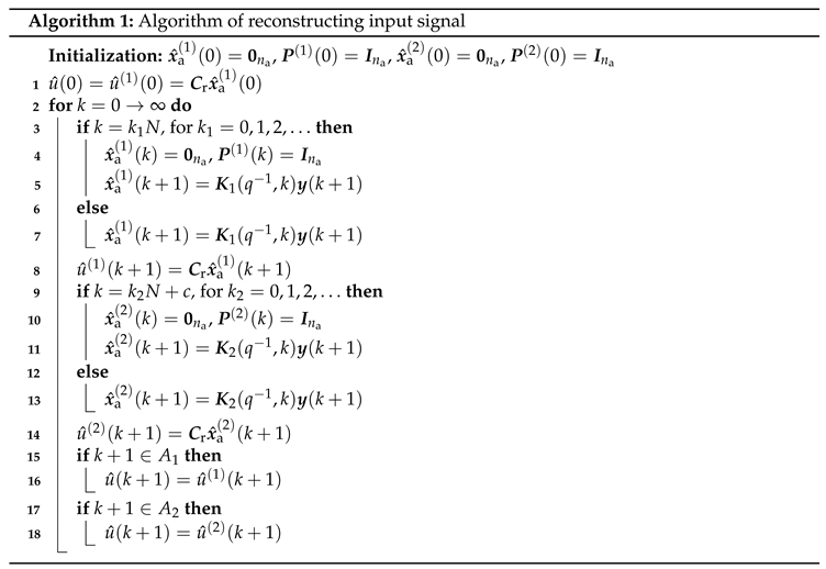
Based on the above analysis, the algorithm of reconstructing the input signal with infinite length can be demonstrated in Algorithm Section 3.2, in which and denote the conceptual time-varying transfer operators of the Kalman filters and , respectively, and the superscripts and are used for distinguishing between and .
4. Numerical Simulation and Analysis
In this section, the proposed input reconstruction approach is validated using two examples. In the first example, a randomly generated system is used for validating the effectiveness of the proposed approach. In the second example, a mass-spring-damper system is used to validate the effectiveness
4.1. Input Reconstruction of a Randomly Generated System
Secondly, choose a white noise sequence with the covariance function with
and then pass it through a 7th-order Butterworth low-pass filter with a cutoff frequency of 300 Hz, afterwards choose the filtered white noise as the input . Additionally,
Thirdly, set , and set the value of to be
Fourthly, choose the sampling period as seconds, and then based on the model (7), the simulated output can be obtained.
Finally, with the simulated output , based on using Algorithm Section 3.2, in which Hz, , , , and seconds, the reconstructed input signal can be obtained.
The input reconstruction results from the step 800 to the step 1400 based on using Algorithm Section 3.2 is illustrated in Figure 4. As seen in Figure 4, by comparing the difference between and , it can be concluded that the proposed input reconstruction approach is effective, and it can be used for a signal with infinite length.
In Figure 5, it can be seen that without the logic block 3 in the proposed approach, merely using or cannot reconstruct the input signal well, especially near the step 1000 and the step 1200.
4.2. Virtual Input Force Sensing
Figure 6 displays a mass-spring-damper system which can be found in many mechanical systems. One common example is the suspension of a car. In this example, the input force u is reconstructed by using the displacement of the mass m, i.e., a virtual input force sensor is formulated using the proposed input reconstruction approach and the data from the displacement sensor measuring the value of .
The following numerical values to the variables m, , and b in the mass-spring-damper system is shown in Table 1.
According to the above values, the continuous-time transfer function between the input u and the output can be obtained:
Transform the continuous-time transfer function into a discrete-time state-space model with the sampling period seconds, then the system matrices of the state-space model can be obtained:
and
Given the input force
where the frequency Hz and the frequency Hz.
Set , and set , and choose the sampling period as seconds, and then based on the model (7), the simulated output can be obtained. Finally, with the simulated output , based on using Algorithm Section 3.2, in which Hz, , , , and seconds, the virtual input force sensor output can be obtained.
The virtual input force sensing results from the step 800 to the step 1400 based on using Algorithm Section 3.2 is illustrated in Figure 7. As seen in Figure 7, by comparing the difference between and , it can be concluded that the proposed input reconstruction approach is effective in the application of virtual sensing.
In Figure 8, it can be seen that without the logic block 3 in the proposed approach, merely using or cannot reconstruct the input signal well, especially near the step 1000 (not obvious) and the step 1200.
According to the applications of Algorithm Section 3.2 in the above examples, direct inversion of the model (7) can be avoided, and only the detectability4 of the model (8) should be guaranteed, and in addition, the proposed approach can avoid the drawbacks in existing indirect system inversion approaches mentioned in Section 1.
5. Conclusions and Perspectives
In this paper, an alternative approach for reconstructing infinite-length signal is proposed, and the proposed approach is prospective method for virtual sensing, sensor linearization and so on. The validation results from two examples can illustrate the effectiveness of the proposed approach. According to both theoretical derivation and numerical studies, it can be known that the proposed approach can avoid all the drawbacks existing in current input reconstruction approaches. However, because of the observability problem of the augmented model (8), the proposed approach can be only used for reconstructing a single input or multiple inputs without spectrum overlapping. In the future, the method will be extended to solve the multiple-input reconstruction problem and the problem of input reconstruction of nonlinear systems. Moreover, the effects from the parameters , N, c, d, , and , and the Kalman filter dimension problem will be explored.
Author Contributions
Conceptualization, R.H.; methodology, R.H.; software, R.H.; validation, R.H.; formal analysis, R.H.; investigation, R.H.; resources, R.H.; data curation, R.H.; writing—original draft preparation, R.H.; writing—review and editing, R.H., C.B. and G.B.; visualization, R.H.; supervision, R.H.; project administration, R.H.; funding acquisition, R.H. All authors have read and agreed to the published version of the manuscript.
Funding
This research was funded by the Natural Science Foundation of Zhejiang pvovince, P.R. China (Grant No. LQ23F030005) and the University Research Development Foundation in Zhejiang A&F University, P.R. China (Grant No. 203402000601).
References
- Lesnic, D. Inverse Problems with Applications in Science and Engineering; CRC Press: Boca Raton, FL, 2022. [Google Scholar]
- Santamarina, J.C.; Fratta, D. Discrete Signals and Inverse Problems: An Introduction for Engineers and Scientists; John Wiley & Sons: Chichester, England, 2005. [Google Scholar]
- Liu, L.; Kuo, S.M.; Zhou, M. Virtual sensing techniques and their applications. In Proceedings of the 2009 IEEE International Conference on Networking, Sensing and Control, Okayama, Japan, 26–29 March 2009; pp. 31–36. [Google Scholar]
- Nagy, J.G.; Plemmons, R.J.; Torgersen, T.C. Iterative image restoration using approximate inverse preconditioning. IEEE Transactions on Image Processing 1996, 5(7), 1151–1162. [Google Scholar] [CrossRef] [PubMed]
- Jung, Y. Inverse System Identification With Applications in Predistortion; Linköping University: Linköping, Sweden, 2018. [Google Scholar]
- Uhl, T. The inverse identification problem and its technical application. Archive of Applied Mechanics 2007, 77(5), 325–337. [Google Scholar] [CrossRef]
- Zhou, K.; Doyle, J.C.; Glover, K. Robust and Optimal Control; Prentice Hall: Englewood Cliffs, NJ, 1996. [Google Scholar]
- Golub, G.H.; Van Loan, C.F. Matrix Computations; John Hopkins University Press: Baltimore, MD, 2012. [Google Scholar]
- Van Zundert, J.; Oomen, T. On inversion-based approaches for feedforward and ILC. Mechatronics 2018, 50, 282–291. [Google Scholar] [CrossRef]
- Devasia, S.; Chen, D.; Paden, B. Nonlinear inversion-based output tracking. IEEE Transactions on Automatic Control 1996, 41(7), 930–942. [Google Scholar] [CrossRef]
- Sogo, T. On the equivalence between stable inversion for nonminimum phase systems and reciprocal transfer functions defined by the two-sided Laplace transform. Automatica 2010, 46(1), 122–126. [Google Scholar] [CrossRef]
- Widrow, B.; Walach, E. Adaptive Inverse Control: A Signal Processing Approach; John Wiley & Sons: Hoboken, NJ, 2008. [Google Scholar]
- Hunt, L.; Meyer, G.; Su, R. Noncausal inverses for linear systems. IEEE Transactions on Automatic Control 1996, 41(4), 608–611. [Google Scholar] [CrossRef]
- Jetto, L.; Orsini, V.; Romagnoli, R. Accurate output tracking for nonminimum phase nonhyperbolic and near nonhyperbolic systems. European Journal of Control 2014, 20(6), 292–300. [Google Scholar] [CrossRef]
- Romagnoli, R.; Garone, E. A general framework for approximated model stable inversion. Automatica 2019, 101, 182–189. [Google Scholar] [CrossRef]
- Gross, E.; Tomizuka, M.; Messner, W. Cancellation of discrete time unstable zeros by feedforward control. Journal of Dynamic Systems, Measurement, and Control 1994, 116, 33–38. [Google Scholar] [CrossRef]
- Tomizuka, M. Zero phase error tracking algorithm for digital control. Journal of Dynamic Systems, Measurement, and Control 1987, 109, 65–68. [Google Scholar] [CrossRef]
- Abd-Elrady, E.; Gan, L.; Kubin, G. Direct and indirect learning methods for adaptive predistortion of IIR Hammerstein systems. Elektrotechnik und Informationstechnik 2008, 125(4), 126–131. [Google Scholar] [CrossRef]
- Fritzin, J.; Jung, Y.; Landin, P.N.; Händel, P.; Enqvist, M.; Alvandpour, A. Phase predistortion of a Class-D outphasing RF amplifier in 90nm CMOS. IEEE Transactions on Circuits and Systems II: Express Briefs 2011, 58, 642–646. [Google Scholar]
- Blanken, L.; Willems, J.; Koekwbakker, S.; Oomen, T. Design techniques for multivariable ILC: Applications to an industrial flatbed printer. IFAC-PapersOnLine, 2016; 49, 213–221. [Google Scholar]
- Hazell, A.; Limebeer, D.J.N. An efficient algorithm for discrete-time H∞ preview control. Automatica 2008, 44(9), 2441–2448. [Google Scholar] [CrossRef]
- Mirkin, L. On the H∞ fixed-lag smoothing: How to exploit the information preview. Automatica 2003, 39(8), 1495–1504. [Google Scholar] [CrossRef]
- Roover, D.D.; Bosgra, O.H. Synthesis of robust multivariable iterative learning controllers with application to a wafer state motion system. International Journal of Control 2000, 73(10), 968–979. [Google Scholar] [CrossRef]
- Bohn, C.; Cortabarria, A.; Härtel, V.; Kowalczyk, K. Active control of engine-induced vibrations in automotive vehicles using disturbance observer gain scheduling. Control Engineering Practice 2004, 12(8), 1029–1039. [Google Scholar] [CrossRef]
- Han, R.; Bohn, C.; Bauer, G. Recursive engine in-cylinder pressure estimation using Kalman filter and structural vibration signal. IFAC-PapersOnLine 2018, 51, 700–705. [Google Scholar] [CrossRef]
- Lewis, F.L.; Xie, L.; Popa, D. Optimal and Robust Estimation: With an Introduction to Stochastic Control Theory; CRC Press: Boca Raton, FL, 2008. [Google Scholar]
| 1 | The system is proper when the degree of the numerator does not exceed the degree of the denominator of its transfer function, otherwise the system is improper. |
| 2 | A system is minimal-realized if and only if it is both controllable and observable. |
| 3 | Actually, the proposed input reconstruction approach is not limited to proper systems, the approach can also be used for improper systems by replacing the present input by future input in (7). |
| 4 | A system is detectable if all the unobservable states are stable. |
Figure 1.
Inverse problems (: input; : output; : inverse system model; : forward system model).
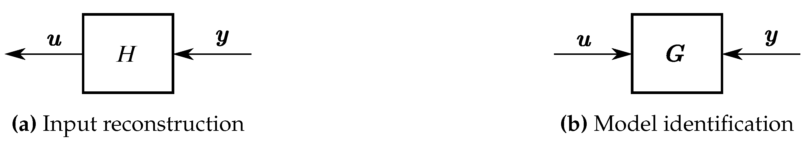
Figure 2.
Timing diagram (c and N are positive integers).
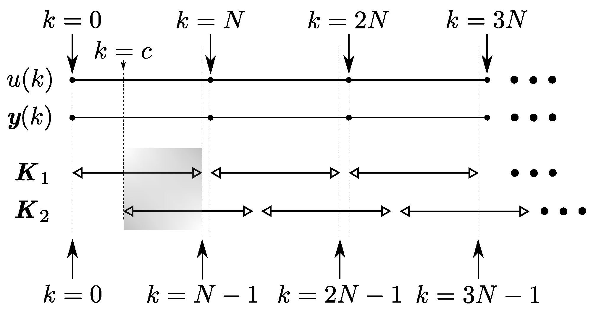
Figure 3.
Input reconstruction (: the first Kalman filter; : the second Kalman filter; : the a priori state estimate; : the a posteriori state estimate; : the a priori error variance; : the a posteriori error variance; : Kalman filter gain; The notation “”: transpose).
Figure 3.
Input reconstruction (: the first Kalman filter; : the second Kalman filter; : the a priori state estimate; : the a posteriori state estimate; : the a priori error variance; : the a posteriori error variance; : Kalman filter gain; The notation “”: transpose).
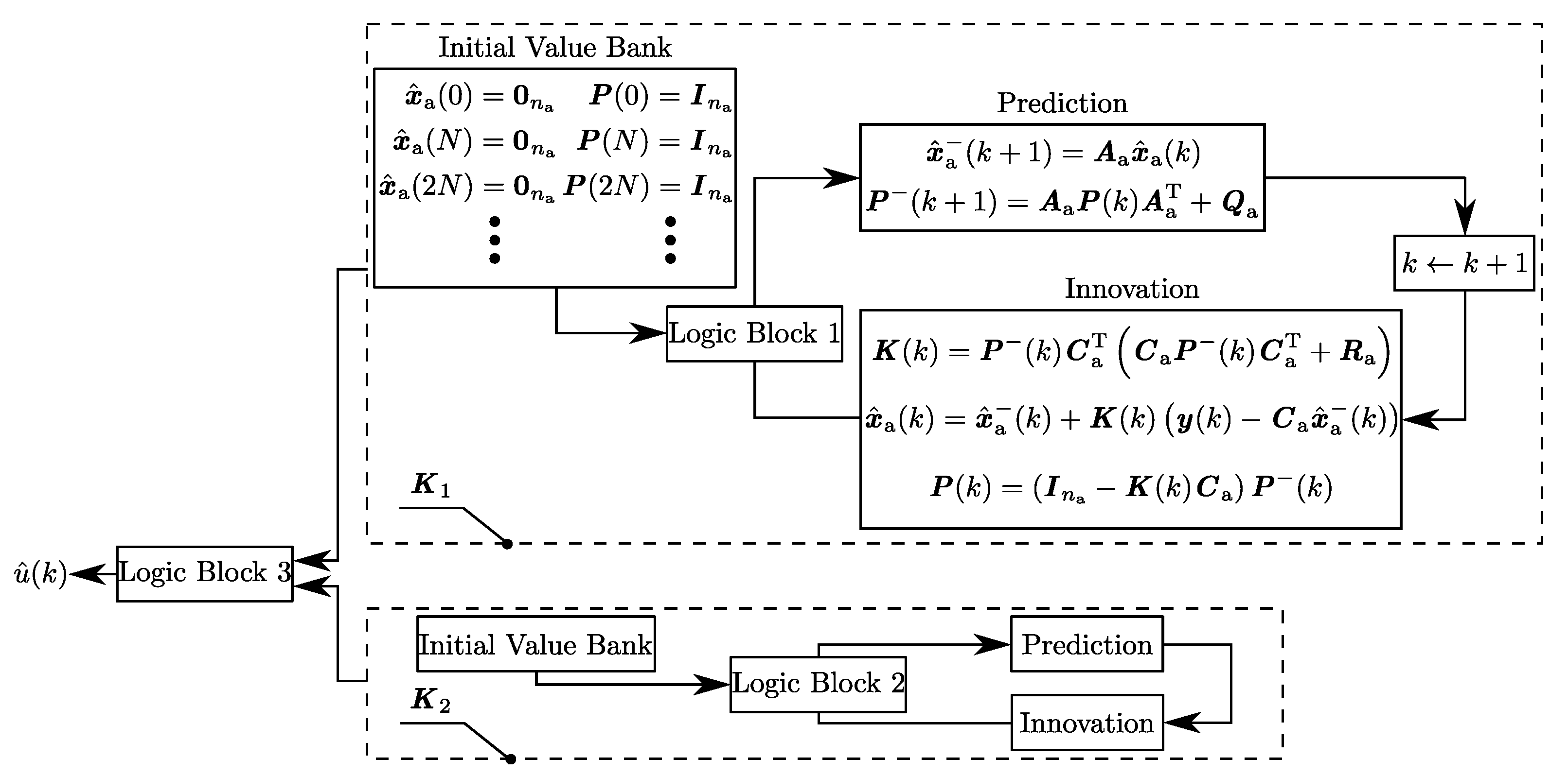
Figure 4.
Reconstructed input.
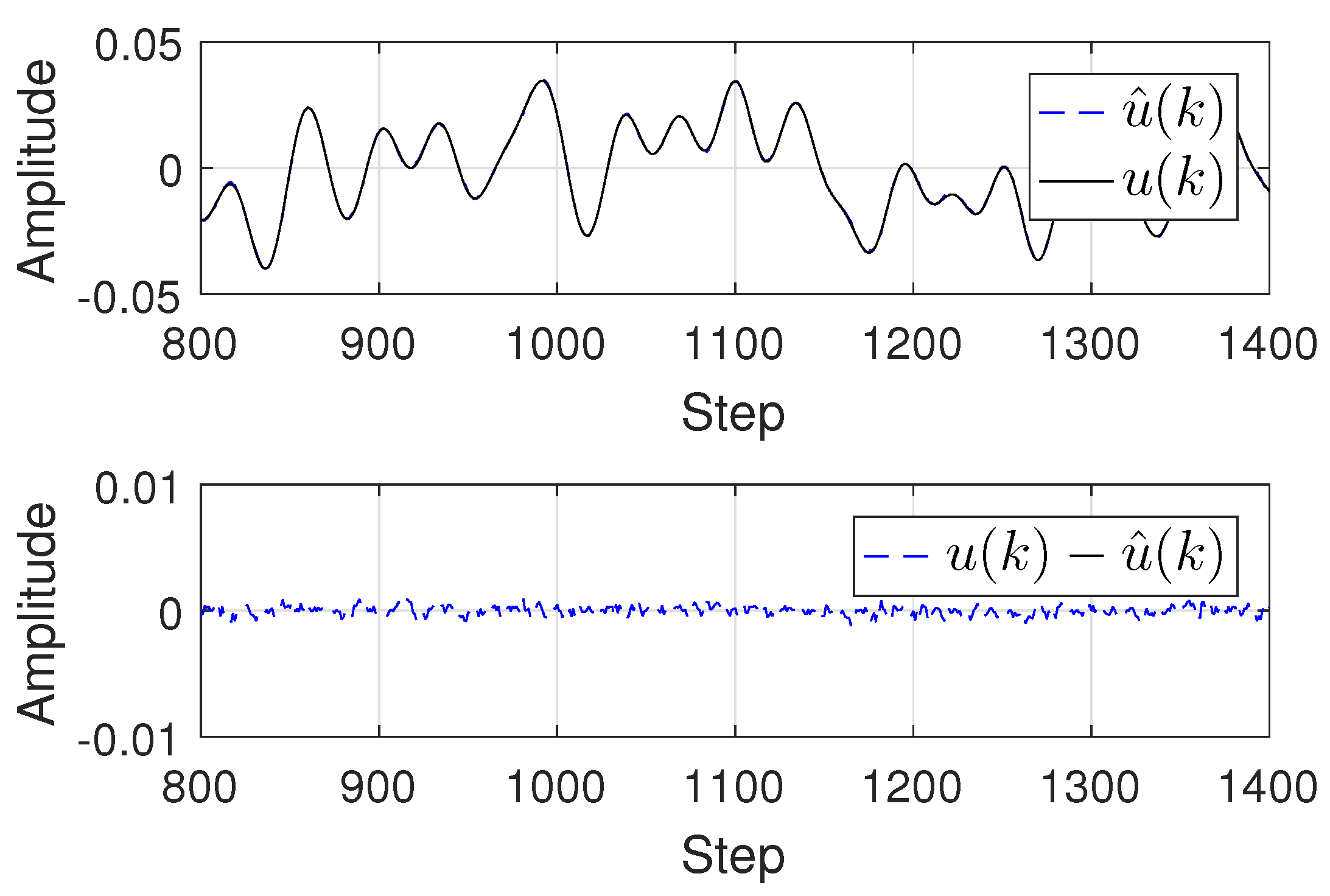
Figure 5.
Input reconstruction results based on using one Kalman filter or .
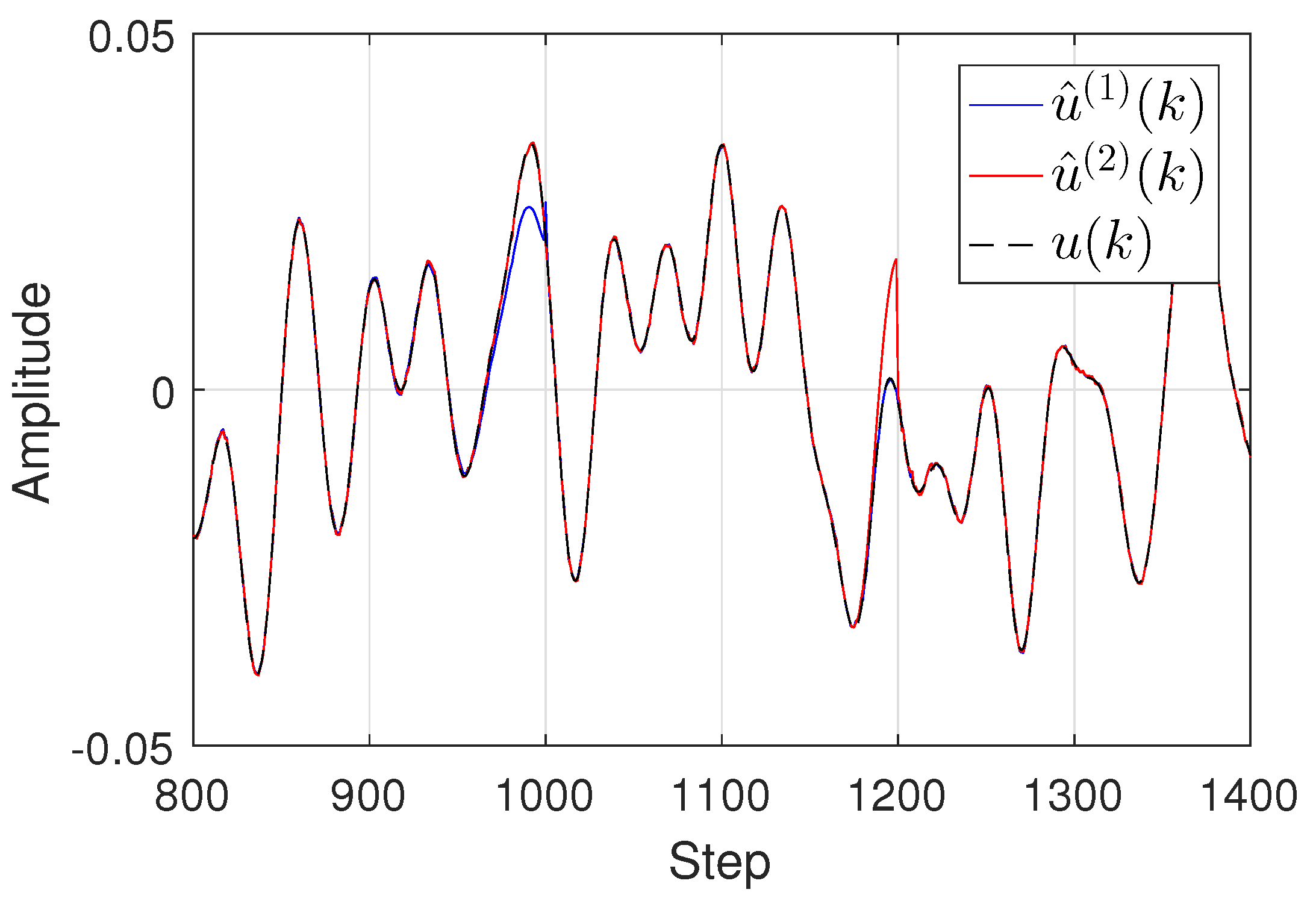
Figure 6.
Mass-spring-damper system (: the spring constant; b: the damping constant; m: the mass; d: the displacement; u: the input force).
Figure 6.
Mass-spring-damper system (: the spring constant; b: the damping constant; m: the mass; d: the displacement; u: the input force).
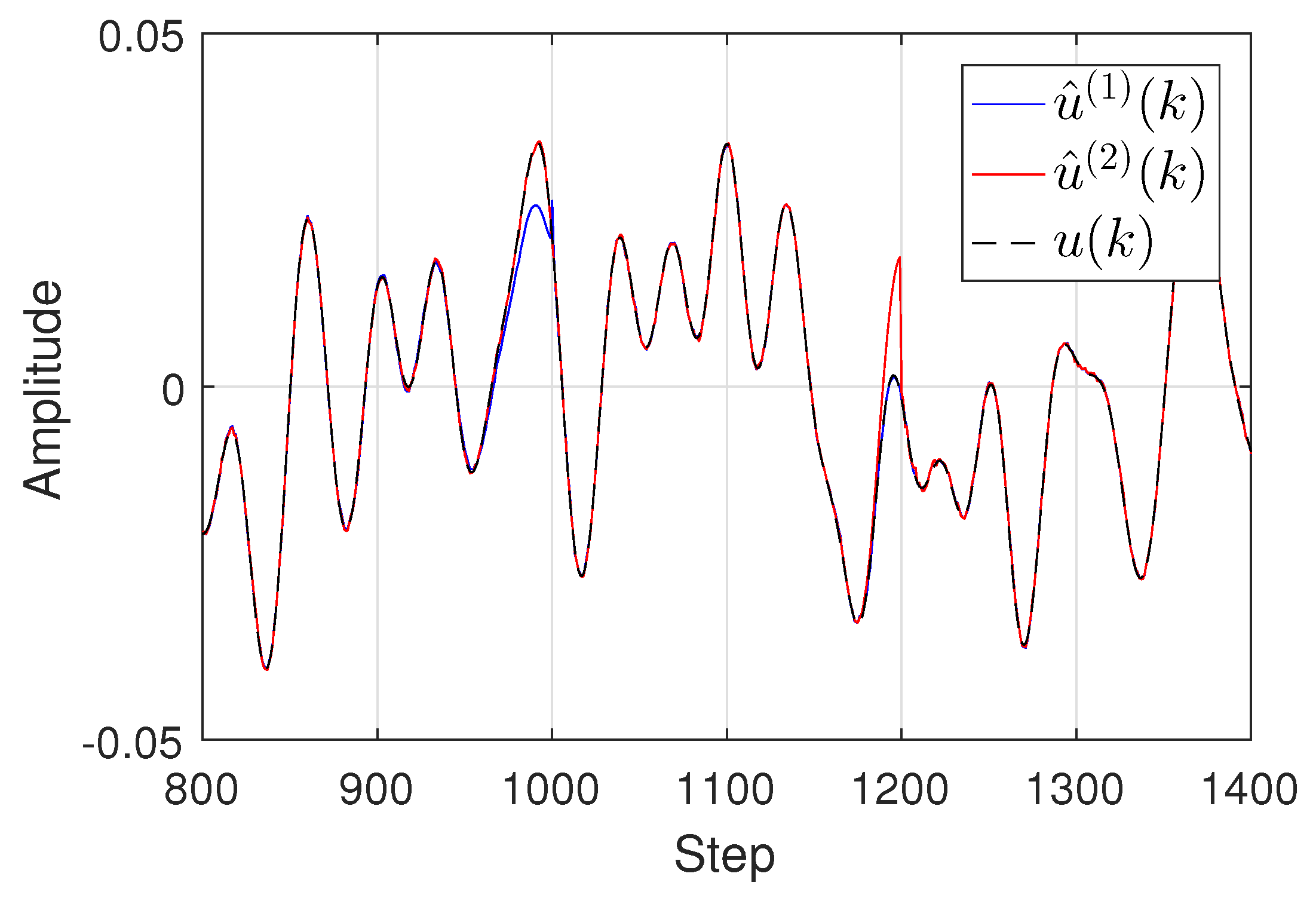
Figure 7.
Output of virtual input force sensor.
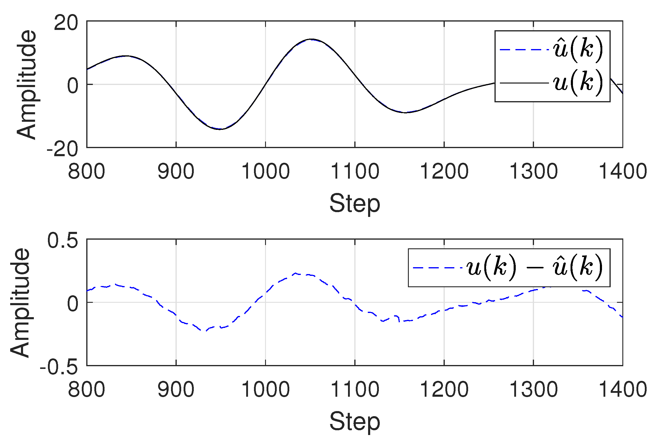
Figure 8.
Virtual input force sensing based on using one Kalman filter or .
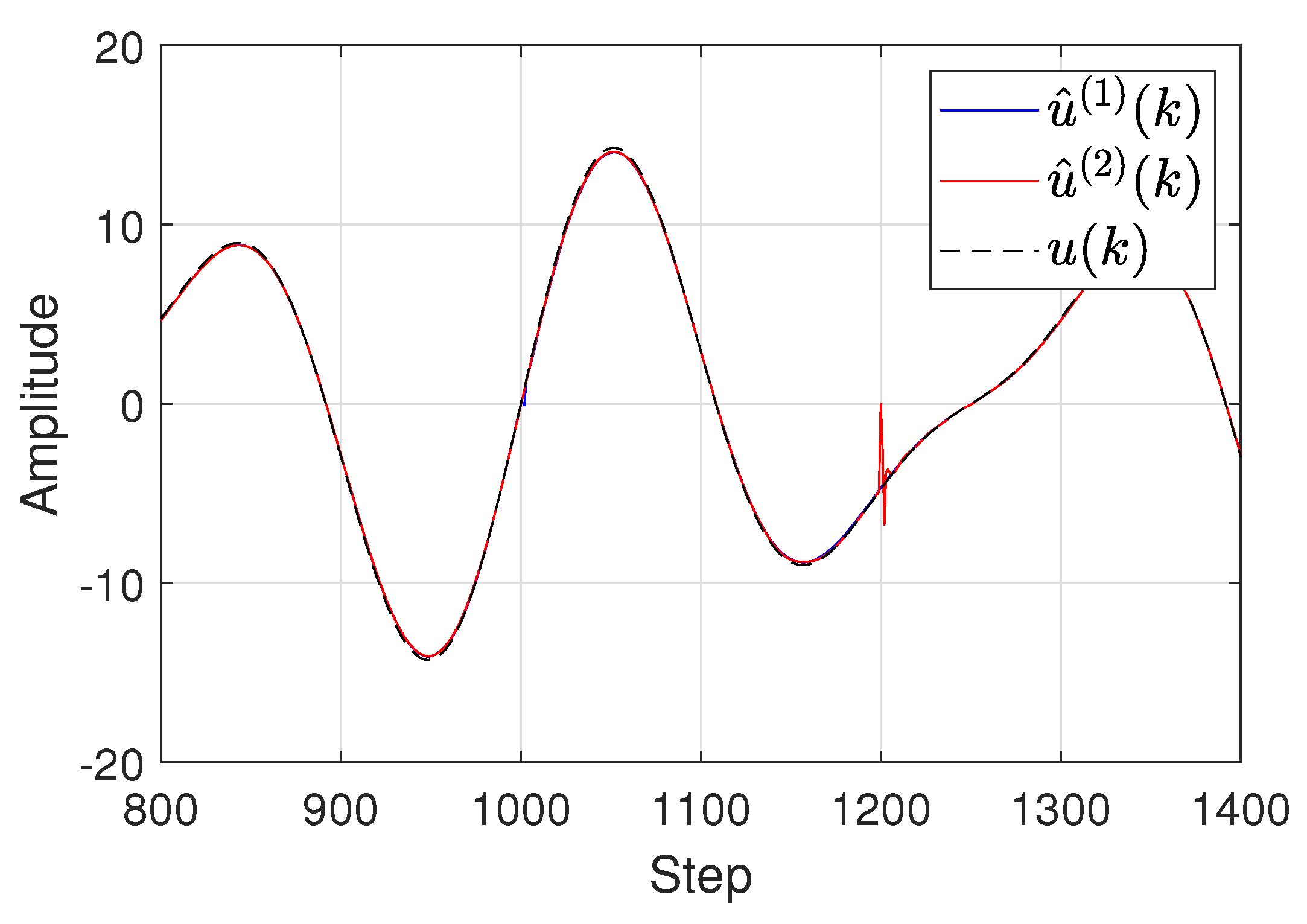

Table 1.
Values of the variables.
| Parameter | Value |
|---|---|
| m | 1.0 kg |
| 1.0 N/m | |
| b | 0.2 Ns/m |
Disclaimer/Publisher’s Note: The statements, opinions and data contained in all publications are solely those of the individual author(s) and contributor(s) and not of MDPI and/or the editor(s). MDPI and/or the editor(s) disclaim responsibility for any injury to people or property resulting from any ideas, methods, instructions or products referred to in the content. |
© 2024 by the authors. Licensee MDPI, Basel, Switzerland. This article is an open access article distributed under the terms and conditions of the Creative Commons Attribution (CC BY) license (http://creativecommons.org/licenses/by/4.0/).
Copyright: This open access article is published under a Creative Commons CC BY 4.0 license, which permit the free download, distribution, and reuse, provided that the author and preprint are cited in any reuse.


