

Submitted:
08 June 2024
Posted:
11 June 2024
You are already at the latest version
Abstract
This study was carried out with a low-cost electronic nose prototype based on eight metal oxide sensors (MQ) in order to characterize samples of lemons treated with 0.5% and 0.1% of sodium benzoate. The MQ sensors designed are sensitive to one or more chemicals to detect the presence of a variety of chemicals in the air. The sensor MQ135 detects ammonia, hydrogen sulphide and benzene. Signal data were studied to obtain a pattern recognition of rotten in lemon fruits. Network analysis was used to obtain a calibration of measures among the stage of lemons. In this article, an electronic nose prototype based on 8 MQ metal oxide sensors has been used in order to analyze and characterize different lemon varieties to which different chemical treatments have been applied in pre-harvest. PCA-based data analyzes were used to observe clusters in the data. Through the combined use of the data obtained by the nose and these Sequential Neural Networks (SNNs) a classification tool for lemon varieties and applied treatments has been obtained. It is shown the ability of this device to be used as a reliable discrimination method, in addition to providing low cost and optimization of time and expert resources.
Keywords:
resistive sensors
; monitoring
; postharvest
; Citrus limon
1. Introduction
eNose devices play a fundamental role when it comes to characterizing samples according to their aroma, being an alternative to conventional sensory methods, as well as gas chromatography techniques [1]. eNose technology is based on a series of non-specific sensors, which react to gases and generate different signals that, once processed for feature extraction, can be used for compound identification and sample classification function of the aromas emitted.
eNose are based on a series of non-specific resistive sensors, which react to gases and generate different signals that, once processed for feature extraction, can be used for compound identification and classification of the samples depending on the aromas emitted [2]. They are capable of detecting complex mixtures of volatile compounds present in gaseous samples. These mixtures generate a combined response in the sensors and create an odor pattern. These devices are capable of detecting complex mixtures of volatile compounds present in gaseous samples. These mixtures generate a combined response in the sensors and create an odor pattern [3].
In this article, an electronic nose prototype based on 8 MQ metal oxide sensors [4,5,6] has been used in order to analyze and characterize different lemon varieties to which different chemical treatments have been applied in pre-harvest.
Numerous studies have been carried out on the application of low-cost electronic nose in different types of substances. One of the most recent studies was applied to Indian tea. Using this technology, it was possible to evaluate different grades of black tea and their qualities, reaching the conclusion that it was a promising device for carrying out tasks related to quality control in the field and at the IAA [7]. Another product where the electronic nose can be applied is the lemon fruit [8,9]. Consumer concerns about food safety are increasing, increasingly demanding products free of pesticides or with very limited use of them. Different investigations have shown that the post-harvest application of additives in different fruits controlled rot caused by the characteristic molds of citrus fruits (Penicillium digitatum and Italicum), such as the treatments of potassium sorbate and sodium benzoate in oranges and lemons [9,10]. However, as far as is known, the application of any of these lemon additives in pre-harvest has not been studied.
The use in the detection of certain properties of the lemon is another of the many applications that the electronic nose has. The lemon tree (Citrus limon (L.) Burm.f.) is a tree belonging to the Rutaceae family. Spain is the main exporter of lemons for fresh consumption worldwide and the leading producer in Europe. Lemon production in Spain is located mainly in the Vega Baja del Segura area (Alicante), Valencian Community and in the Region of Murcia. The cultivars that predominate in these areas are known as ‘Fino’, whose harvest begins in March and ends in July, and ‘Verna’, whose harvest begins in October and ends in February [11].
Citrus are prone to develop numerous physiological skin disorders, or skin spots, which are manifested through different morphological symptoms that can appear before or after harvest. The incidence of these symptoms depreciates the external quality of the fruit and is one of the main factors of postharvest losses, as well as rejection by the consumer in the market [8]. To control these postharvest diseases, fungicides or synthetic waxes are usually applied pre- and postharvest, which contain ammoniacal and/or chemical compounds [thiabendazole, imazalil, among others] [12]. However, there are more and more consumer concerns about food safety, increasingly demanding products free of pesticides or with a very limited use of these.
Food additives are substances that are intentionally added to food for a technological purpose. Different investigations have shown that the post-harvest application of these substances in different fruits controlled the rot caused by the characteristic molds of citrus fruits (Penicillium digitatum and italicum), such as the potassium sorbate and sodium benzoate treatments in oranges and lemons [9,10]. However, as far as is known, the application of any of these pre-harvest lemon additives has not been studied. The use of electronic noses for the detection of these additives is a non-destructive technique that allows to qualitatively distinguish different fruit samples for their subsequent classification and treatment, in a fast way.
The use of data analysis, such as principal component analysis (PCA), cluster analysis, and classification techniques such as artificial neural networks (ANN) or support vector machines (SVM), has the potential to accurately classify samples based on of its aroma (Gutiérrez-Osuna, 2002). Currently, numerous studies have been carried out on the application of low-cost electronic nose in different samples. The analysis of Indian tea using this technology allowed the evaluation of different grades of black tea and its qualities, reaching the conclusion that it was a promising device for the execution of tasks related to quality control in the field and in the IAA [7].
The objective of this paper is testing the use of a prototype of an electronic nose to obtain a rot recognition pattern in lemon fruits. In this way, a non-destructive quick method to differentiate the pre-harvest additives of “Fino” and “Verna” lemons in whole pieces of fruit will be presented. PCA-based data analyzes were used to observe clusters in the data. Through the combined use of the data obtained by the nose and these Sequential Neural Networks (SNNs) a classification tool for lemon varieties and applied treatments has been obtained. It demonstrates the ability of this device to be used as a reliable discrimination method, in addition to providing low cost and optimization of time and expert resources. Network analyzes were used to obtain a calibration of the measurements [13].
2. Materials and Methods
The experiment began on December 14, 2022 and ended on January 12, 2023. Ten control samples were initially measured with an electronic nose. Subsequently, 5% and 0.1% sodium benzoate samples were measured. The treatments are shown in Table 1. Lemons of the ‘Fino’ and ‘Verna’ varieties were used, provided by the company Citrus Gea Belmonte S.L., located in Torreagüera (Murcia) Spain, which cultivated this variety on a commercial plot located in the north of Murcia.
For the application of the treatments in the field (Table 1), 8 lemon trees were randomly selected. This application was carried out by foliar spraying (15 total liters per treatment) and up to 4 times at one-month intervals. The last applications were carried out a week before harvest, which occurred at its optimal stage of commercial ripening.
Where the treatments are the next. CNT (control), distilled water was added; BS0, 5 (5% sodium benzoate, solution of 75 g BS, 1.5 L water, 15 mL wetting agent); BS0, 1 (0.1% sodium benzoate, 150 g BS, 1.5 L water, 15 mL wetting agent). They were prepared for application in the field to the already selected trees, except for the control, since it only consisted of distilled water. Data of the specific concentrations are detailed in section 2.2.
2.1. Experimental Design and Storage Conditions
The lemons were transferred to the laboratory immediately after harvesting, where they were organized into different batches of 10 lemons according to the applied treatment. This classification was carried out visually based on size, color and appearance, in order to obtain a homogeneous sample that did not present visually perceptible defects. The cold storage conditions were in cold rooms at 8°C and 80-85% relative humidity (RH). The characterization of the fruits took place through the low-cost prototype of the eNose and this was carried out on the days following receipt of the fruits in the laboratory until reaching a week of analysis with each one. of the varieties (approximately 1 month of testing).
For the application of the treatments, 6 trees were randomly selected for the ‘Fino’ variety and the same number for the ‘Verna’ variety. This cited application was made by foliar spraying (15 liters in total per treatment) and the times that these were applied were 4 at intervals of one month. The last applications were carried out 7 days before harvest, which took place in its commercial maturation stage; on February 17, 2022 for the ‘Fino’ variety and on May 26, 2022 for the ‘Verna’ variety.
The lemons were transferred to the laboratory immediately after their collection, where they were organized in different batches according to the variety and the treatment applied. The ‘Fino’ variety lemons were randomly classified into 7 batches of 10 pieces per treatment, as well as the ‘Verna’ variety lemons, at the time of harvest. Said classification was carried out visually based on size, color and appearance, in order to obtain a homogeneous sample that did not present visible defects. Cold storage conditions were: 8°C and 80-85% relative humidity (RH). The determinations of the volatile organic compounds (VOCs), through the low-cost prototype of eNose, were carried out on the days following the receipt of the fruits in the laboratory until reaching one week of analysis with each one of the varieties.
2.2. Formulation of Treatments
The application of the treatments was distributed over the lemon trees in the field, with a total of 6 different treatments for each of the varieties, in addition to the control. The solutions were prepared by dissolving 75, 150 and 450 grams (g) of sodium benzoate in 1.5 liters (L) of water and 75, 150 and 450 g of potassium sorbate in 1.5 L of water, in order to obtain 15 L total solutions at concentrations of 0.5, 1, and 3%, respectively. Likewise, 15 mL of ecological wetting agent were added to the solutions to improve adhesion. These solutions were applied in the field recently formulated, although the control trees of both varieties were not sprayed. Table 2
Where, CNT (control), distilled water was added; BS0, 5 (5% sodium benzoate, solution of 75 g BS, 1.5 L water, 15 mL wetting agent); BS0, 1 (0.1% sodium benzoate, 150 g BS, 1.5 L water, 15 mL wetting agent). They were prepared for application in the field to the already selected trees, except for the control, since it only consisted of distilled water. Details of the specific concentrations are detailed in section 2.2.
2.3. Determination of Volatile Organic Compounds Using a Low-Cost Prototype of an eNose
The tests, for each of the lemon varieties, took place the days after the receipt of the fruits in the laboratory, using a low-cost electronic nose (EN) prototype. The prototype was designed by the technology-based company TeleNatura, in collaboration with the work group of the Engineering Department of the Miguel Hernández University (UMH), Spain. The device included a simple sample delivery system, which consisted of a chamber where the samples were deposited, together with a fan, as well as an array of sensors and a microcontroller unit (Arduino Nano microcontroller with USB serial connection; Figure 1).
The same design was used in works such as the identification of La Rioja wine varieties [4], the detection of the lethal bronzing disease in palm trees [5] and the discrimination between a range of types of olive oil [6]. The sensor array consisted of eight MQS sensors (MQ-135, MQ-2, MQ-3, MQ-4, MQ-5, MQ-7, MQ-8, and MQ-9), manufactured by Hanwei Electronics. Co., Ltd. (Zhengzhou, China), which had resistors (RL) that changed their values depending on the mixture of gases present in them (Table 3).
The variation of the voltage across these resistances introduces the modulation of the heating of the sensor. Said device works with an Arduino Nano microcontroller to generate the voltage signals introduced into the sensors and measure their responses, together with an analog circuit, made up of a DAC and operational amplifiers to control the heating of the sensors. Data sheets for some sensors (MQ7 and MQ9 in particular) recommend switching between two heater voltages (5.0 V and 1.4 V) in a 60 + 90 s cycle, with 90 s sensor response to end of interval. This can significantly improve sensitivity as it is now possible to detect the sensor at different operating temperatures. EN is built to be able to vary the voltage input to the sensors. In the present investigation, the voltage was varied sinusoidally with a period of 128 s, with values ranging from 1.6 to 4.8 V and a total of 256 steps in each period. The sample chamber of the device was a glass chamber and was connected by a 6 mm PVC tube, through PG7 nylon cable glands, to a separate PP5 (food grade polypropylene) detection chamber, which contained the sensor assembly. Likewise, another tube returned to the sample chamber, completing a hermetically closed circuit.
To normalize the outputs of the MQ sensors, 50 kΩ trim pots were used as load resistors, with the pot values adjusted until the sensor channels gave a voltage difference of less than 100 mV, at least half an hour after introduce the sample. Likewise, the impedance characteristics of each sensor were balanced, since this produced a degree of normalization to counteract the variability produced during their manufacture.
The analysis of the samples through the EN began for the ‘Fino’ variety on February 21, 2022 and for the ‘Verna’ variety on May 30, 2022, these dates being the appropriate ones due to the seasons of harvest of each of the varieties. The investigation was carried out from the beginning of the analyzes to the completion of one week with both lemon varieties, ensuring that the 10 samples from each batch were measured at least once.
All experiments were carried out in a clean and disinfected environment. First, the EN sensors were exposed to ambient air for 30 minutes. Next, the analysis of the samples began, which consisted of introducing each of the ten pieces of the chosen batch into a glass jar of X mL capacity (sample chamber). Once the fruit was inside the sample chamber, it was hermetically closed, leaving the sensors included in the relevant lid exposed to the sample in question for a period of 10 minutes (Figure 2: lid and sensors). After this time, and before introducing a second sample, the device chamber is cleaned. For this, it is left exposed to ambient air for 20 minutes. At all times, the sensors were prevented from having direct contact with the sample to avoid possible saturations in the measurements. All samples analyzed and ambient air exposures from the sensors are manually recorded in self-developed software before starting to measure. Said software was intended to connect the device at low cost (EN) to a computer with a minimum of 64 bits, in order to obtain the data analyzed during the day, generate Excel files (.xls), which contained the data of each of daily measurements, and perform analysis of raw data for extraction characteristics.
2.4. Electronic Nose Data Analysis
To analyze the raw data, the first step is to perform feature extraction. The Discrete Fourier Transform (DFT) was used to extract the frequency coefficients of each temporal signal from each sensor. For this, the same internal software mentioned above was used. A total of 80 coefficients are extracted for each sample, forming a feature vector together with a label that is later stored and used for classification. The entire data analysis process is included in Figure 2.
Second, Principal Component Analysis (PCA) is used to reduce the dimensionality of the data from 80 to 2. In this way, 2D plots can be created in which each point represents one of the analyzed samples. This tool allows us to look at sample pools and select a subset of coefficients that we will use for classification. In this case, we chose to use 40 coefficients, whose retained variability was >= 95%. The PCA and the graphical representation were executed using the Python® language, using the sklearn and matplotlib libraries.
The results of 3 classification algorithms are compared below. One of them is unsupervised, k-nearest-neighbors (k-nn) and the other two are supervised, Sequential Neural Networks (SNN) and support vector machines (MVS). The objective is to see which algorithms classify the results better, hypothesizing that the supervised models will outperform the unsupervised one, and that with the best of these it will be possible to obtain a fast data classification tool, which together with the analysis device will provide the ability to easily, reliably and quickly analyze large data sets.
The k-nearest-neighbors (k-nn) algorithm is used, which is an approximation to data classification that estimates the probability that a data point belongs to one group or another based on the group in which the data are found. closest data points. This algorithm classifies in an unsupervised way, that is, it does not make use of the labels that we generate. Instead, it generates labels from the grouping of the data based on the distances of each sample to a series of clusters. Comparing the labels generated by the algorithm with the original ones from the samples, we can measure the classification capacity of the k-nn.
Models based on supervised learning have been trained in order to obtain a tool for rapid data classification. A first group of models are based on SNN sequential neural networks. Hyperparameter tuning is an essential step in machine learning to ensure that the model performs optimally and is suitable for real-world applications. The process can be time consuming, but it can significantly improve model performance and make it more robust to new data. The hyperparameter adjustment process was carried out randomly and they were chosen based on the results on a validation set. 80% of the data from all the analyzes carried out so far were used to train them and the remaining 20% to perform a validation of the model. The models are trained to return an estimate of the probability that they belong to each of the categories into which the samples have been divided. We assume that the group with the highest probability is the output of the model.
Finally, the feature vectors extracted and processed by PCA are classified using models based on support vector machines (SVM). Support Vector Machines (SVMs) are a type of machine learning algorithm used for classification and regression analysis. C and gamma are two important parameters used in SVMs. C is a regularization parameter that controls the tradeoff between low training error and low test error, while gamma controls the shape of the decision bound. A small value of gamma will result in a decision boundary with a larger radius and a smoother decision surface, while a large value of gamma will result in a more complex decision surface that may overfit the training data. The optimal values of C and gamma can be determined using a grid search or random search process to get the best performance of the SVM model on the given data set. This process involves testing different combinations of C and gamma values and evaluating the model’s performance on a validation data set, selecting the values that produce the highest accuracy or lowest error rate. To generate and train the models, optimal values for C and gamma are sought. Using a recursive code with k-fold 5 and 20% trial values, C and gamma values are obtained with a score of 0.94. The data is then divided into training and test groups with proportions of 80-20%, respectively. For the binary classification between infected and non-infected, no particular classifier is specified. For classification among the four types of infection, a onevsone (ovo) multiclassifier was used.
For the analysis of results, confusion matrices are made for each of the models through which the total precision of the models, their sensitivity and specificity are calculated. The maximum, minimum and mean values are calculated in a 10-fold testing process.
Accuracy = number of hits / total number of predictions
For cases of binary classification, the measures are also used:
Sensitivity = number of positive hits / (number of positive predictions)
Specificity = number of negative hits / (number of negative predictions)
3. Results
Initially, the results of the experiments carried out on the Fino lemon variety are shown, then the results of those carried out on the Verna variety, and finally, both varieties are compared together.
The passage given deals with the analysis of the differentiation capacity of the electronic nose between lemons treated with various chemical products and untreated lemons of the Fino variety. The samples were divided into three groups labeled as B, S (potassium sorbate) and C (control without treatment), with the main objective of testing the ability of the electronic nose to differentiate between these groups. Figure 2 shows a representation of the first two Principal Components (PC) obtained from the analysis (on the right). However, it can be seen that the three established groups cannot be clearly distinguished visually in the graph on the left. On the right side of Figure 2, the k-nearest neighbors (k-nn) algorithm was used, which formed three clusters that do not correspond to the established labeling.
Subsequently, the labeled data is entered into the two supervised models used, and Table 4 shows a comparison of the results of the 3 used algorithms.
Secondly, a detailed analysis of the classification of the data according to the treatment and the concentration of the applied product is offered. In this case, there were a total of seven labels, including two treatments with three concentrations each and one control treatment. The labels of each of the groups were B05, B1, B3, S05, S1, S3 and C.
To effectively classify the data, a single model was used, and the results obtained are presented in Table 5. The Support Vector Machine (SVM) algorithm obtained the best results, outperforming the Stochastic Neural Network (SNN) algorithm by 10 points in terms of mean classification precision. However, the only area where SNN outperformed SVM was in the minimum accuracy score, beating it by one point. In contrast to the previous case, there was a considerable difference between the maximum and minimum precision scores, which amounted to 88 points.
For the last algorithm (SVM), a confusion matrix was elaborated in Figure 3.
In this passage the results of an experiment carried out with the Verna variety are analyzed. The main objective of the analysis was to evaluate the classification capacity of the different treatments used. However, since no control treatment was used in the experiments, only two sets of tags, B (sodium benzoate), S (potassium sorbate), were generated.
To achieve the desired objective, a principal component analysis was performed, and the results were visualized in the form of a scatter diagram, where the two principal components (PC) that explain 80% of the total variance were represented. As shown in Figure 5, the samples treated with Sodium Benzoate are clustered on the left of the graph, while the samples treated with Potassium Sorbate are clustered on the right. This clear differentiation between both groups can be seen reflected in the classification capacity of the k-nn algorithm. While in the previous cases with this algorithm a 35 and 12 percent classification is obtained, for the Verna variety 100% accuracy was obtained in all attempts. Results of the other algorithms are not shown since for all cases a 100% classification was obtained without variability between passes.
Below, a comparison among varieties (Verna, Fino 49 and Fino 95) is presented. For this, firstly an analysis is shown to evaluate the differentiation capacity of these two varieties. Figure 6 represents the PCA analysis using the first two principal components that carry 75% of the variability of the data. A clear differentiation of the Fino groups is observed in purple on the left and Verna in yellow and on the right.
Moreover, kmeans algorithm obtains a 100% of precission in the binary classification for Fino and Verna varieties. Additionally, it is demonstrated that, Verna varieties were subdivided in two groups (purpple and blue).
The difference among treatments is presented in Figure 7. In this figure, the influence of the applied treatments was very important in Verna varieties. This situation was not similar in Fino variety.
Finally, a new PCA analysis for Verna variety about difference of treatments is presented in Figure 8. In this case, further analysis with a kmeans algorithm was obtained a precision of 100% about the classification among groups.
4. Discussion
Overall, the results obtained from this analysis provide valuable information on the limitations of the electronic nose in accurately distinguishing between treated and untreated lemons of both varieties (Fino and Verna). New research can help optimize the chemical treatment process and its impact on the Fino variety, which will result in better quality and higher yields.
The results obtained from this analysis highlight the effectiveness of the SVM algorithm to accurately classify data based on treatment and concentration. The large difference in precision scores between the best and worst performing groups underscores the need to carefully consider the selection of treatments and concentrations for the Verna variety. These findings may help optimize the cultivation and production processes of this crop, leading to better yields and improved quality. Other studies lead to discriminating table olives with negative olfactory defects caused by abnormal fermentation during the product manufacturing process or even establish a PLS regression between the E-nose data with sensory aroma evaluated [14].
The results obtained from the analysis indicate that the two treatments have significantly different effects on the Verna variety. The grouping of the samples treated with Sodium Benzoate and Potassium Sorbate separately suggests that the treatments have different and specific effects on the variety. Postharvest development of Botrytis cinerea in tomatoes were discriminated using an electronic nose during 8 days of storage at ambient temperature [15].
In general, this analysis provides valuable information on the effects of the different treatments on the Verna variety, which can be useful to optimize the cultivation and production processes of this crop.
In Figure 6, which shows the labeled PCA analysis according to the two study varieties, a clear differentiation is presented. The ability of the nose to distinguish between lemon varieties is shown. In addition, it can be seen that on the right the group corresponding to Verna and clearly separated from Fino, is subdivided into 2 groups. This is corresponding to the two treatments applied to the samples. This leads us to think that in Verna’s experiment the influence of the chemicals applied to the nose was much higher than in the case of Fino. This could also explain the difference observed with respect to the varieties. To evaluate this effect, more experiments with a larger number of samples should be carried out. The ability of the different sensors of the electronic equipment to discriminate the olfactory pattern of the samples to be analyzed is an aspect to be noted that allows the discrimination of samples with different sensory profiles. In fact, in the literature there are a lot of studies to lead to discriminate food properties in coffee [1,12,17], virgin olive oil [18], table olives [14] or tomatoes [19]. This researchers were able to classify samples according to chemical compounds with electronic devises.
The electronic nose has served to differentiate additive treatments in two varieties of lemon. There are differences between the varieties and within the varieties, the treatments within each variety are clearly distinguished. With a few small adjustments it is possible to use the electronic nose to distinguish the pre-harvest treatments in lemon. This makes it possible to obtain a qualitative rapid measurement system.
The data generated, from eNose, after the analysis of the lemons, were analyzed by PCA and classified using kmeans and SVM models.
It was observed that, for all the classifications generated, the models yielded more than 80% accuracy, which demonstrated that it is possible to differentiate, through eNose technology, the different varieties of lemons, as well as their treatments. and concentrations.
5. Conclusions
It is observed that the maximum variability is found between lemons and not between treatments, since the results show greater precision in the classification by samples, this being 100%. The average precision of treatments ranges around 80%.
The electronic nose has detected changes in varieties, concentrations and treatments. It can be concluded that it has functioned adequately as a detector of volatile organic compounds related to the different preharvest treatments to reduce rot in these citrus fruits.
The PCA analysis and the neural network are able to discriminate the samples. They can be properly used for real-time analysis if some cloud data management system is added.
Neural networks are capable of discriminating samples. They can be properly used for real-time analysis if a cloud data management system is added.
It would remain pending to carry out an experiment over time to detect the evolution of volatile organic compounds related to fruit rot.
Author Contributions
Conceptualization, A.R.C., G.M.M. and A.C.C.; methodology, A.R.C., G.M.M., A.C.C. and I.C.F.; software, A.C.C. and M.J.O.; validation, A.R.C., G.M.M., A.C.C. and I.C.F.; formal analysis, A.R.C., G.M.M., A.C.C. and I.C.F.; investigation, A.R.C., G.M.M., A.C.C. and D.M.V.; resources, A.R.C. and D.M-V.; data curation, A.R.C., G.M.M., A.C.C. and I.C.F.; writing—original draft preparation, A.R.C., G.M.M., A.C.C. and D.M-V.; writing—review and editing, A.R.C., G.M.M., A.C.C. and D.M-V.; visualization, A.R.C., G.M.M., A.C.C. and D.M-V.; supervision, A.R.-C., and D.M-V.; project administration, A.R.-C., and D.M-V.; funding acquisition, A.R.-C., and D.M-V. All authors have read and agreed to the pub-lished version of the manuscript.
Funding
This research was funded by CDTI project, IDI-20211216 PRE-HARVEST ANALYSIS OF FOOD ADDITIVES TO CONTROL ROT AND IMPROVE QUALITY IN LEMON, Spanish Ministry of Science and Innovation, in collaboration with Citrus Gea Belmonte S.L. company.
Institutional Review Board Statement
Not applicable.
Informed Consent Statement
Not applicable.
Data Availability Statement
Data available on request.
Acknowledgments
The authors are grateful for the funding of the CDTI project IDI-20211216 PRE-HARVEST ANALYSIS OF FOOD ADDITIVES FOR THE CONTROL OF ROTS AND IMPROVEMENT OF QUALITY IN LEMON’ and within it, in the section “Application of electronic nose in pre-harvest research of additives “food products to control rot and increase quality in lemon.” This was in collaboration with Citrus Gea Belmonte S.L. company.Without this support, the research could not have been carried out.
Finally, we appreciate the support provided by the company TELENATURA EBT, S.L. in the technological development of the electronic nose prototypes used in the experiment.
Conflicts of Interest
The authors declare no conflict of interest.
References
- Barea-Ramos, J.D.; Cascos, G.; Mesías, M.; Lozano, J.; Martín-Vertedor, D. Evaluation of the Olfactory Quality of Roasted Coffee Beans Using a Digital Nose. Sensors 2022, 22, 8654. [Google Scholar] [CrossRef] [PubMed]
- Cascos, G.; Barea-Ramos, J.D.; Montero-Fernández, I.; Ruiz-Canales, A.; Lozano, J.; Martín-Vertedor, D. Burn Defect and Phenol Prediction for Flavoured Californian-Style Black Olives Using Digital Sensors. Foods 2023, 12, 1377. [Google Scholar] [CrossRef] [PubMed]
- Gutierrez-Osuna, R. Pattern analysis for machine olfaction: a review. IEEE Sensors J. 2002, 2, 189–202. [Google Scholar] [CrossRef]
- Celdrán, A.C.; Oates, M.J.; Cabrera, C.M.; Pangua, C.; Tardaguila, J.; Ruiz-Canales, A. Low-Cost Electronic Nose for Wine Variety Identification through Machine Learning Algorithms. Agronomy 2022, 12, 2627. [Google Scholar] [CrossRef]
- Oates, M.J.; Abu-Khalaf, N.; Molina-Cabrera, C.; Ruiz-Canales, A.; Ramos, J.; Bahder, B.W. Detection of Lethal Bronzing Disease in Cabbage Palms (Sabal palmetto) Using a Low-Cost Electronic Nose. Biosensors 2020, 10, 188. [Google Scholar] [CrossRef] [PubMed]
- Oates, M.J.; Fox, P.; Sanchez-Rodriguez, L.; Carbonell-Barrachina. A.; Ruiz-Canales, A. DFT based classification of olive oil type using a sinusoidally heated, low cost electronic nose. Comput. Electron. Agric. 2018, 155, 348–358. [Google Scholar] [CrossRef]
- Banerjee, M.B.; Roy, R.B.; Tudu, B.; Bandyopadhyay, R.; Bhattacharyya, N. Black tea classification employing feature fusion of E-Nose and E-Tongue responses. J. Food Eng. 2019, 244, 55–63. [Google Scholar] [CrossRef]
- Zacarias, L.; Cronje, P.J.; Palou, L. 2020. Postharvest technology of citrus fruits. In The genus citrus (pp. 421-446). Woodhead Publishing.
- Palou, L.; Usall, J.; Smilanick, J.L.; Aguilar, M.; Viñas, I. Evaluation of food additives and low-toxicity compounds as alternative chemicals for the control of Penicillium digitatum and Penicillium italicum on citrus fruit. Pest Manag. Sci. 2002, 58, 459–466. [Google Scholar] [CrossRef] [PubMed]
- Montesinos-Herrero, C.; del Río, M. .; Pastor, C.; Brunetti, O.; Palou, L. Evaluation of brief potassium sorbate dips to control postharvest penicillium decay on major citrus species and cultivars. Postharvest Biol. Technol. 2009, 52, 117–125. [Google Scholar] [CrossRef]
- Perez-Perez, J.; Castillo, I.P.; Garcia-Lidon, A.; Botia, P.; Garcia-Sanchez, F. Fino lemon clones compared with the lemon varieties Eureka and Lisbon on two rootstocks in Murcia (Spain). Sci. Hortic. 2005, 106, 530–538. [Google Scholar] [CrossRef]
- Palou, L.; Smilanick, J.L.; Montesinos-Herrero, C.; Valencia-Chamorro, S.; Pérez Gago, M.B. (2011). Novel approaches for postharvest preservation of fresh citrus fruits. Citrus Fruits: Properties, Consumption and Nutrition, Nova Science Publishers, Inc., NY, USA, 1.
- Álvarez-Ortí, M.; Pardo, J.E.; Cascos, G.; Sánchez, R.; Lozano, J.; Martín-Vertedor, D. E-Nose Discrimination of Almond Oils Extracted from Roasted Kernels. Nutrients 2023, 15, 130. [Google Scholar] [CrossRef] [PubMed]
- Sánchez, R.; Boselli, E.; Fernández, A.; Arroyo, P.; Lozano, J.; Martín-Vertedor, D. Determination of the Masking Effect of the ‘Zapateria’ Defect in Flavoured Stuffed Olives Using E-Nose. Molecules 2022, 27, 4300. [Google Scholar] [CrossRef] [PubMed]
- Barea-Ramos, J.D.; Rodríguez, M.J.; Calvo, P.; Melendez, F.; Lozano, J.; Martín-Vertedor, D. Inhibition of Botrytis cinerea in tomatoes by allyl-isothiocyanate release from black mustard (Brassica nigra) seeds and detection by E-nose. Food Chemistry 2024, 432, 137222. [Google Scholar] [CrossRef] [PubMed]
- Rodríguez, J.C.; Duran, C.M.; Reyes, A.X. 2009. Electronic Nose for Quality Control of Colombian Coffee Through the Detection of Defects in “Cup Tests”PROCEEDINGS OLFACTION AND ELECTRONIC NOSE, PROCEEDINGS Volume1137, Page 455-456.
- Gardner, J.; Shurmer, H.; Tan, T. Application of an electronic nose to the discrimination of coffees. Sensors Actuators B: Chem. 1992, 6, 71–75. [Google Scholar] [CrossRef]
- Gila, D.M.M.; García, J.G.; Bellincontro, A.; Mencarelli, F.; Ortega, J.G. Fast tool based on electronic nose to predict olive fruit quality after harvest. Postharvest Biol. Technol. 2020, 160, 111058. [Google Scholar] [CrossRef]
- Hong, X.; Wang, J.; Qi, G. E-nose combined with chemometrics to trace tomato-juice quality. J. Food Eng. 2015, 149, 38–43. [Google Scholar] [CrossRef]
Figure 1.
A prototype EN with eight metal-oxide semiconductors (MOSs).
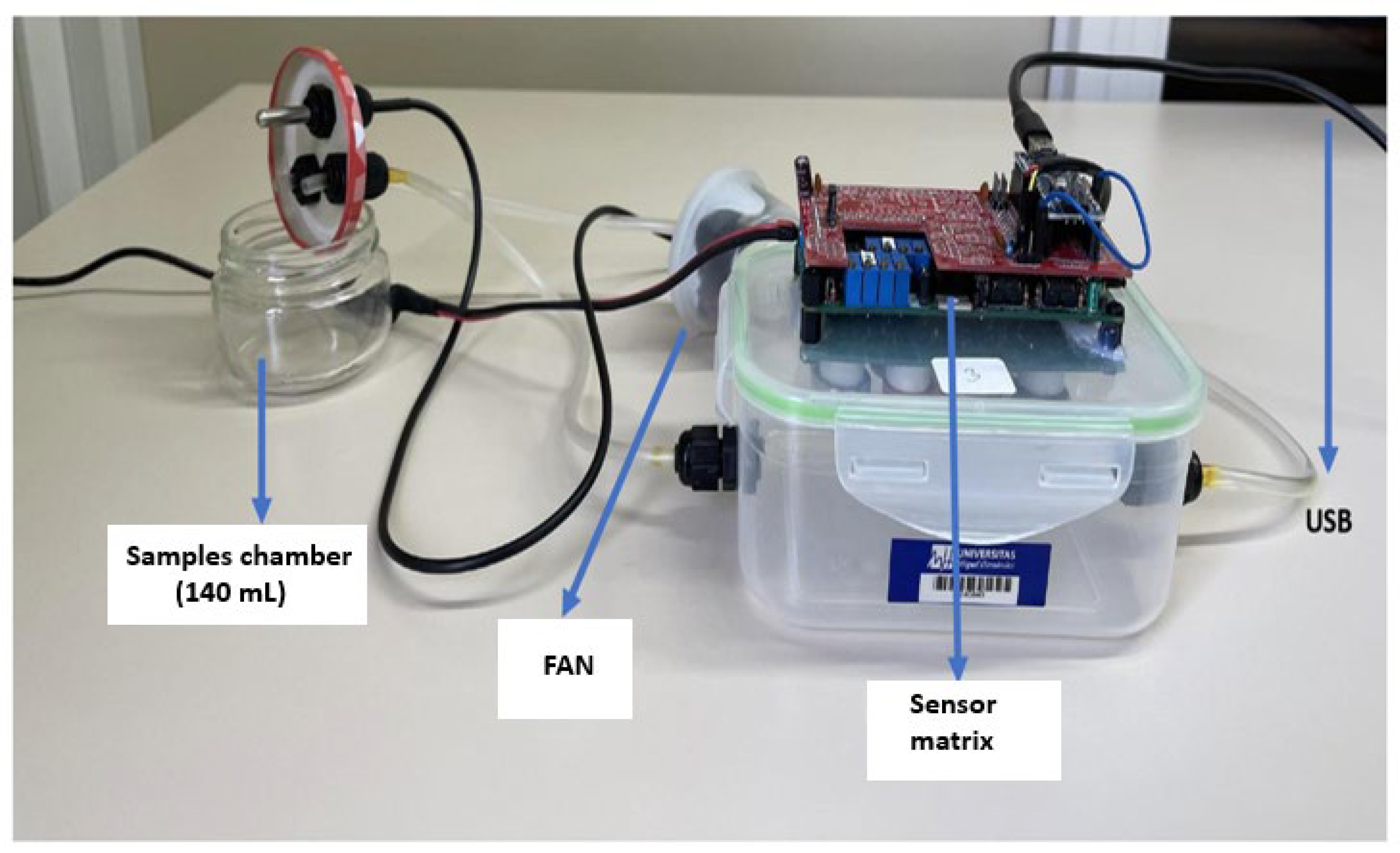
Figure 2.
Main processes for classification of honeys by enose in the experiment.

Figure 3.
Representation of the first two principal components of the data set in both varieties (Fino and Verna). Each point represents one of the samples used and is labeled according to the legend B (sodium benzoate), S (potassium sorbate) and C (control without treatment). On the left is the original labeling of the samples and on the right the labeling performed by the k-nn algorithm.
Figure 3.
Representation of the first two principal components of the data set in both varieties (Fino and Verna). Each point represents one of the samples used and is labeled according to the legend B (sodium benzoate), S (potassium sorbate) and C (control without treatment). On the left is the original labeling of the samples and on the right the labeling performed by the k-nn algorithm.
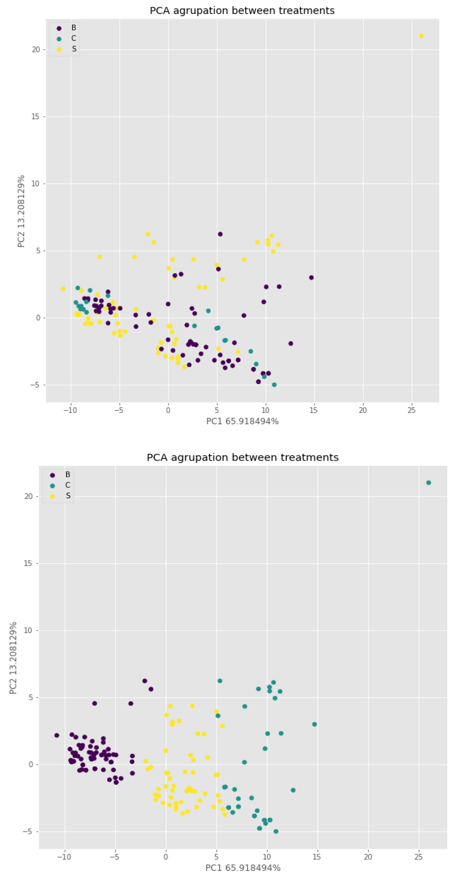
Figure 4.
Confusion matrix of the SVM algorithm for the classification by type of treatment and concentration. Each number on axes 0-6 corresponds to the corresponding label B05, B1, B3, S05, S1, S3, C.
Figure 4.
Confusion matrix of the SVM algorithm for the classification by type of treatment and concentration. Each number on axes 0-6 corresponds to the corresponding label B05, B1, B3, S05, S1, S3, C.
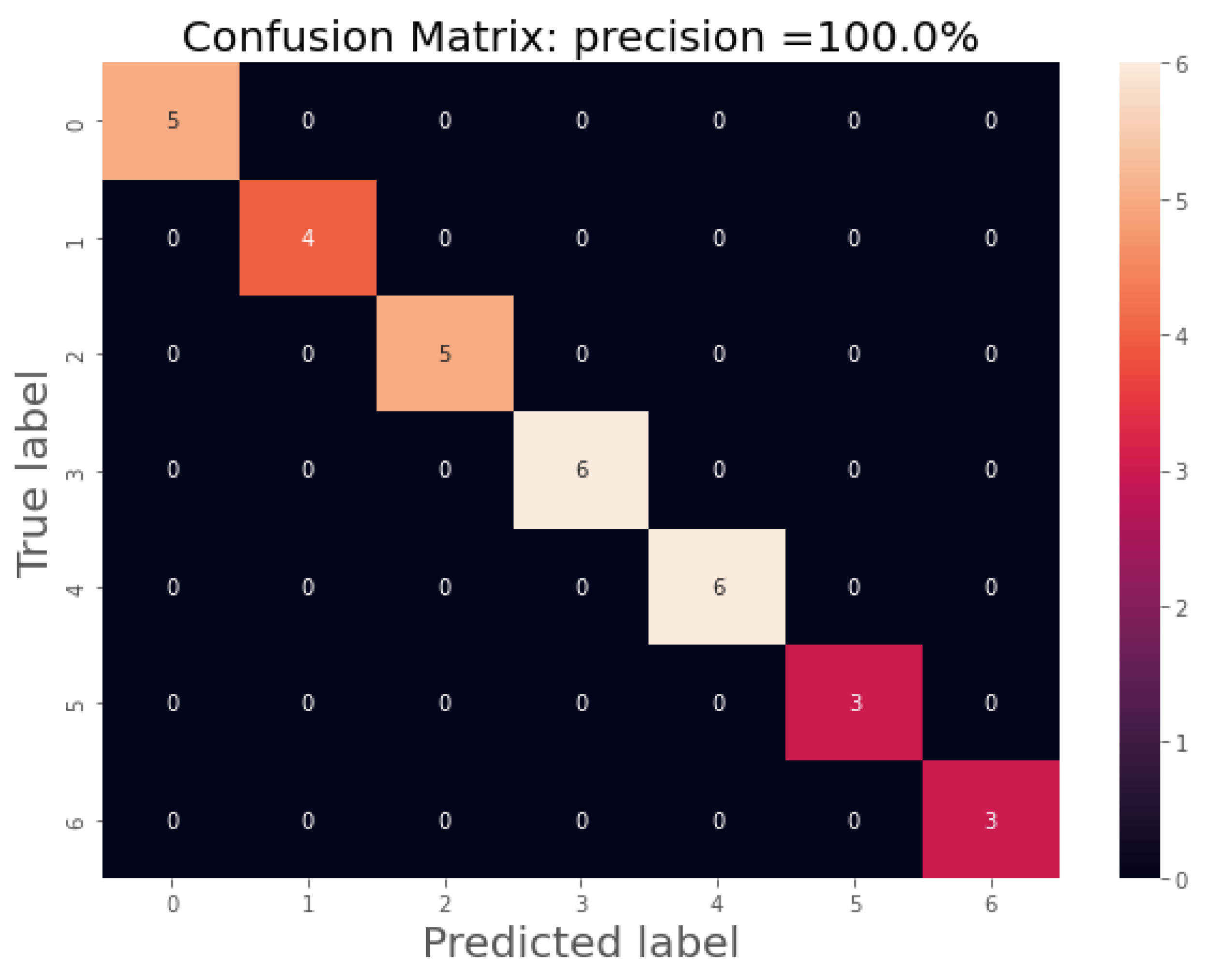
Figure 5.
Representation of the first two principal components of the data set. The grouping of the data is shown according to the 2 treatments applied B (sodium benzoate) and S (potassium sorbate). Each point represents one of the samples used and they are labeled according to the legend.
Figure 5.
Representation of the first two principal components of the data set. The grouping of the data is shown according to the 2 treatments applied B (sodium benzoate) and S (potassium sorbate). Each point represents one of the samples used and they are labeled according to the legend.
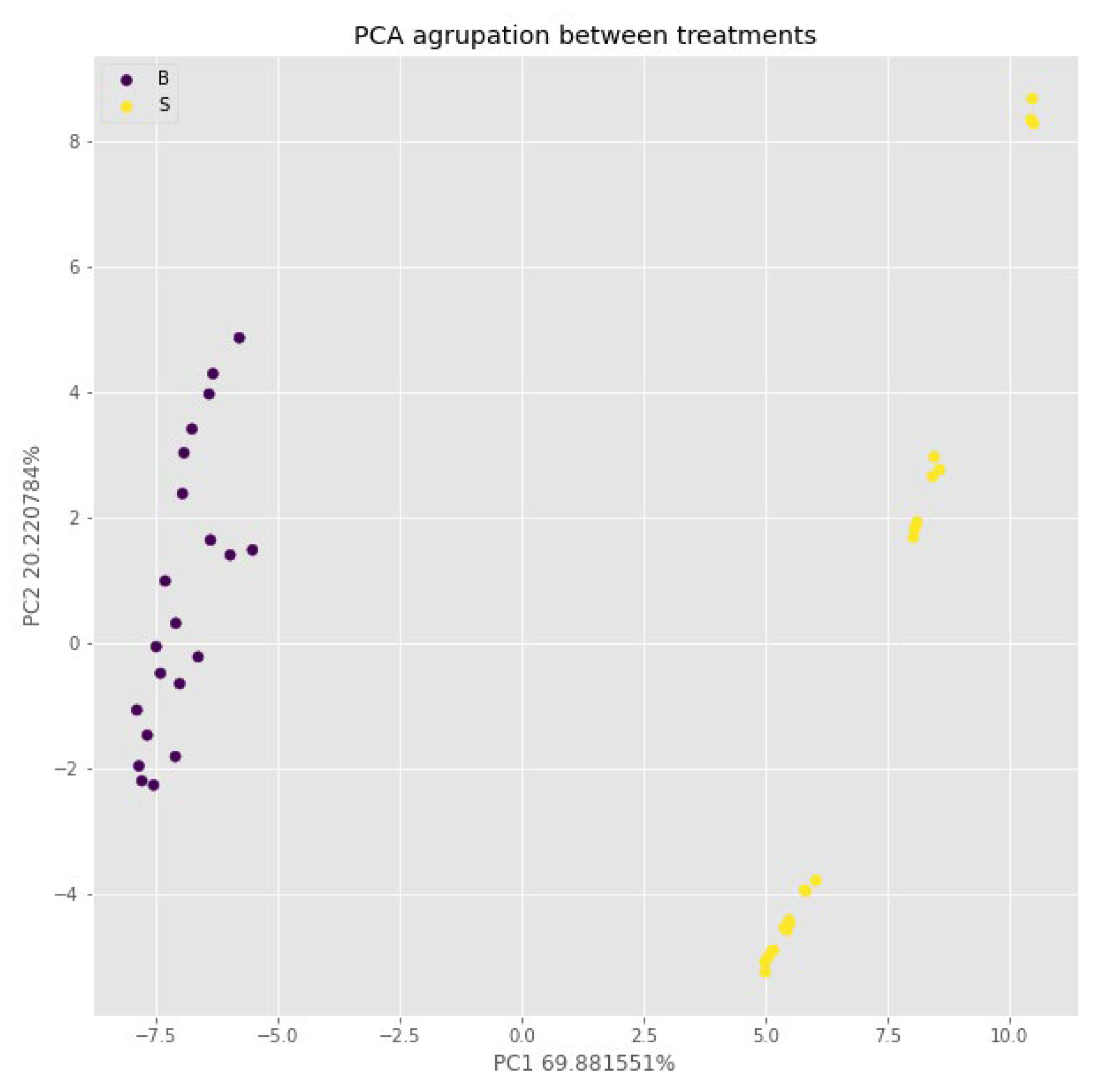
Figure 6.
Representation of the first two principal components of the data set. The grouping of the data is shown according to the two different varieties (Fino 49 and Fino 95, purple and blue in color and Verna, yellow in color). Each point represents one of the samples used and is labeled according to the legend.
Figure 6.
Representation of the first two principal components of the data set. The grouping of the data is shown according to the two different varieties (Fino 49 and Fino 95, purple and blue in color and Verna, yellow in color). Each point represents one of the samples used and is labeled according to the legend.
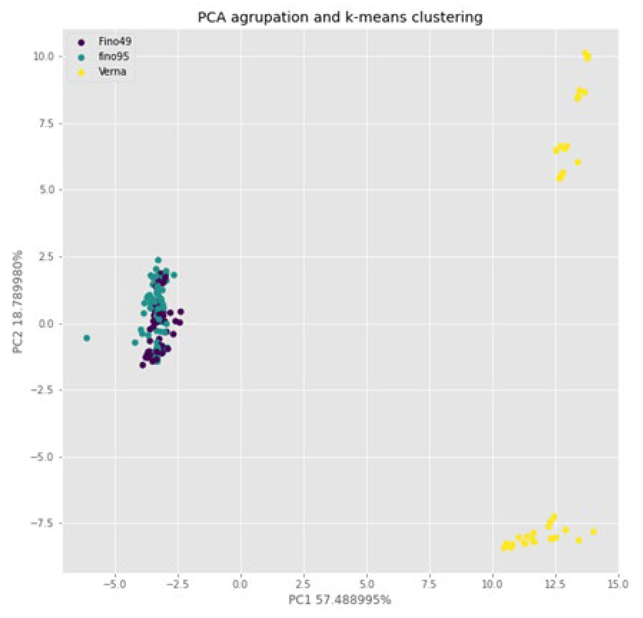
Figure 7.
Representation of the influence of treatments of the data set in Verna variety. The grouping of the data is shown according to the three treatments: B (sodium benzoate), S (potassium sorbate) and C (control).
Figure 7.
Representation of the influence of treatments of the data set in Verna variety. The grouping of the data is shown according to the three treatments: B (sodium benzoate), S (potassium sorbate) and C (control).
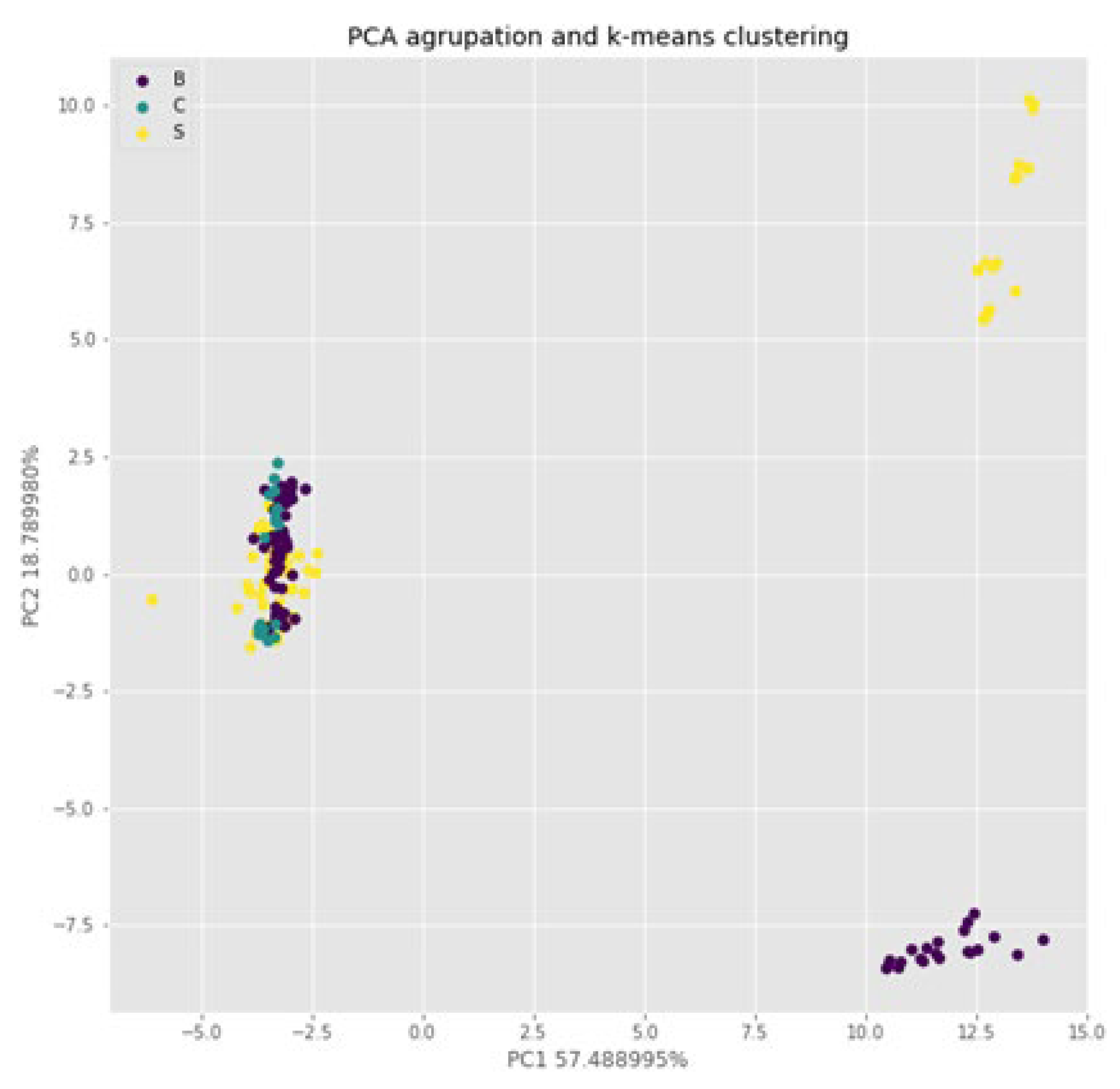
Figure 8.
Representation of the influence of treatments of the data set in Verna variety. The grouping of the data is shown according to the two treatments: B (sodium benzoate), S (potassium sorbate).
Figure 8.
Representation of the influence of treatments of the data set in Verna variety. The grouping of the data is shown according to the two treatments: B (sodium benzoate), S (potassium sorbate).
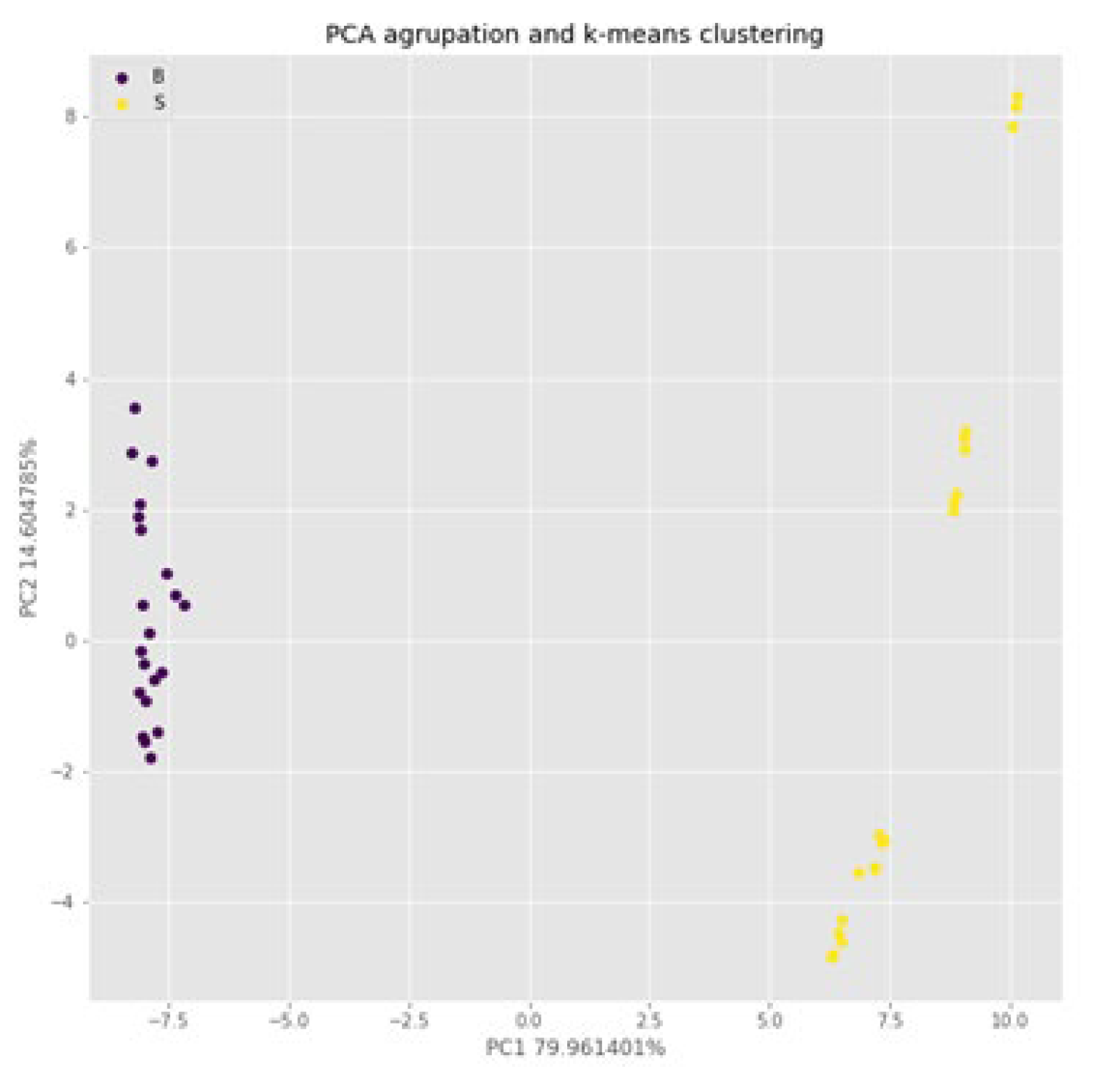

Table 1.
Experimental treatments.
| Treatment | Repetitions | Number of lemons | Number of rotten | Replaced |
|---|---|---|---|---|
| CNT | 10 | 10 | 0 | 0 |
| BS0, 5x1 | 10 | 10 | 0 | 0 |
| BS0, 5x2 | 10 | 10 | 0 | 0 |
| BS0, 5x3 | 10 | 10 | 0 | 0 |
| BS0, 5x4 | 10 | 10 | 0 | 0 |
| BS0, 1x1 | 10 | 10 | 0 | 0 |
| BS0, 1x2 | 10 | 8 | 2 | 9 and 10 |
| BS0, 1x3 | 10 | 6 | 4 | 7, 8, 9 and 10 |
| BS0, 1x4 | 10 | 7 | 3 | 8, 9 and 10 |
Table 2.
Used treatments during the experiment.
| Treatment | Abbreviation | Composition |
|---|---|---|
| Control | Concentration | Distilled water |
| Sodium benzoate 0.5% | BS 0.5% | 75 g BS + 1.5 L water + 15 mL wetting |
| Sodium benzoate 1.0% | BS 1.0% | 150 g BS + 1.5 L water + 15 mL wetting |
| Sodium benzoate 3.0% | BS 3.0% | 450 g BS + 1.5 L water + 15 mL wetting |
| Potassium sorbate 0.5% | PS 0.5% | 75 g PS + 1.5 L water + 15 mL wetting |
| Potassium sorbate 1.0% | PS 1.0% | 150 g PS + 1.5 L water + 15 mL wetting |
| Potassium sorbate 3.0% | PS 3.0% | 450 g PS + 1.5 L water + 15 mL wetting |
Table 3.
Used sensors in the used e-nose prototype and their sensibilities.
| Nº | Sensor | Sensible to |
|---|---|---|
| 1 | MQ2 | LPG (Liquefied Petroleum Gases), Hydrogen and Propane |
| 2 | MQ3 | Alcohol |
| 3 | MQ4 | Methane |
| 4 | MQ5 | Hydrogen and LPG |
| 5 | MQ7 | Hydrogen and carbon monoxide |
| 6 | MQ8 | Hydrogen |
| 7 | MQ9 | Carbon monoxide and liquefied petroleum gases (LPG) |
| 8 | MQ135 | NH3 (ammonia), NOx, alcohol, benzene, smoke, CO2, etc. |
Table 4.
Comparison of the results of the algorithms used for the classification by treatment in Fino variety. The precision value is calculated through a 10-fold testing process from which the maximum and minimum mean value is extracted. The total computing time used by each of the algorithms for training and validation is also shown.
Table 4.
Comparison of the results of the algorithms used for the classification by treatment in Fino variety. The precision value is calculated through a 10-fold testing process from which the maximum and minimum mean value is extracted. The total computing time used by each of the algorithms for training and validation is also shown.
| Algorithm | Average precision [%] | Minimal precision [%] | Maximum precision [%] | Time [s] |
|---|---|---|---|---|
| k-nn | 35.60 | 28.30 | 44.65 | <1 |
| SNN | 90.62 | 81.25 | 100 | 125 |
| SVM | 91.25 | 78.12 | 100 | <1 |
Table 5.
Comparison of the results of the algorithms used for the classification by treatment and concentration. The precision value is calculated through a 10-fold testing process from which the maximum and minimum mean value is extracted. The total computing time used by each of the algorithms for training and validation is also shown.
Table 5.
Comparison of the results of the algorithms used for the classification by treatment and concentration. The precision value is calculated through a 10-fold testing process from which the maximum and minimum mean value is extracted. The total computing time used by each of the algorithms for training and validation is also shown.
| Algorithm | Average precision [%] | Minimal precision [%] | Maximum precision [%] | Time [s] |
|---|---|---|---|---|
| k-nn | 12.45 | 5.03 | 22.64 | <1 |
| SNN | 75.62 | 9.46 | 90.62 | 119 |
| SVM | 85.94 | 8.18 | 100 | <1 |
Disclaimer/Publisher’s Note: The statements, opinions and data contained in all publications are solely those of the individual author(s) and contributor(s) and not of MDPI and/or the editor(s). MDPI and/or the editor(s) disclaim responsibility for any injury to people or property resulting from any ideas, methods, instructions or products referred to in the content. |
© 2024 by the authors. Licensee MDPI, Basel, Switzerland. This article is an open access article distributed under the terms and conditions of the Creative Commons Attribution (CC BY) license (http://creativecommons.org/licenses/by/4.0/).
Copyright: This open access article is published under a Creative Commons CC BY 4.0 license, which permit the free download, distribution, and reuse, provided that the author and preprint are cited in any reuse.


