Submitted:
03 June 2024
Posted:
05 June 2024
You are already at the latest version
Abstract
This paper presents a comprehensive analytical-numerical algorithm constructed for proprotor performance evaluation, focusing on accommodating large inflow angles. The algorithm’s design, range, and analytical features are clarified, indicating its potential to improve performance analysis, particularly for blades with substantial pitch variations. The Stahlhut model has not been validated against the conventional BEMT small-inflow angle methodology. This paper implements a modified Stahlhut model, coupled with the conventional BEMT theory. Preliminary validations of the model demonstrate promising results, with deviations reduced to -3% to 4% compared to conventional BEMT methods exhibiting deviations as high as 20% to 88% against experimental data for a highly twisted proprotor. The reconsideration of the computational module carries considerable implications for the design and refinement of proprotors, providing alternative analysis methods that could improve operational effectiveness across a range of flight scenarios. Drawing upon the theoretical framework presented by Stahlhut, the algorithm enables a more complex understanding of proprotor dynamics, facilitating accurate predictions of the loads at each blade section. The introduced algorithm emerges as a valuable asset for evaluating proprotor performance during the early stages of design and certification, offering both low computational cost and medium to high reliability.
Keywords:
BEMT
; airfoil interpolation
; proprotor performance
; inflow angle
1. Introduction
The Blade Element Momentum Theory (BEMT) emerged as one of the pioneering modeling frameworks for proprotors, offering a practical method to assess the performance of propellers and rotors, particularly in hover and axial flow conditions [1]. Widely utilized in the preliminary stages of proprotor design [2,3], BEMT represents the standard approach for early design processes. To maintain reliability, the conventional BEMT methodology is built up with compressibility corrections [4], Prandtl’s tip-loss method [5], and considerations for rotational effects [6,7], aiming to address real-world complexities that may have been oversimplified in the original theory. More sophisticated techniques involve inviscid surface methods like panel methods coupled with free wake vortex lattice methods (FWVLM) or Computational Fluid Dynamics (CFD), which offer enhanced resolution of the overall flow field but incur higher computational costs [8,9].
Several adaptations have extended BEMT to account for non-zero incidence angles and nonuniform inflow around the azimuth [10]. Another approach, allowing BEMT to consider large inflow angles, has been proposed by Stahlhut [11], which serves as the theoretical foundation of this paper. Alternative methods like BET incorporating dynamic inflow models [1,12] offer precise aerodynamic forecasts for edgewise flight [13], delivering detailed flow-field data beyond the propulsor disk. This flexibility enables the assessment of diverse operational conditions and the exploration of geometric variables, facilitating the creation of internal optimization processes [12,13] to adjust system trimming or modify proprotor geometry to meet specific performance criteria. The trimming is generally executed by the RPM of the proprotor and a combination of collective and feathering [16,17]. The possibility to assess the performance of proprotors with low computational costs for varying geometrical definitions has become more relevant with the introduction of novel designs for emerging fields such as Urban Air Mobility (UAM) [18] and Unmanned Aerial Vehicles (UAV) [19] applications which operate at non-conventional flight regimes.
Conventional BEMT models, commonly found in literature and low-to-medium fidelity tools, are constrained by simplifications in the numerical process, often requiring iterative methods for resolution [20]. These limitations stem from assumptions such as the insignificance of out-of-plane velocity () compared to the in-plane velocity (), small induced angles, and the dominance of the local lift () over drag () components, at each blade section [21]. In contrast, Stahlhut [11] introduced an alternative approach that discards small angle assumptions, explicitly includes in-plane velocity components, and does not assume negligible drag relative to lift, avoiding linearized simplifications and iterative procedures. Fundamentally, the conventional BEMT provides a simplified framework for comprehending the intricate dynamics of fluid-structure interaction. This framework involves a dual decomposition: radial separation of blades and the fluid column into blade elements. It includes a conceptual division between a macroscopic component, following the Momentum Theory, and a local planar component, adhering to the Blade Element Theory.
This paper aims to propose a proprotor algorithm that combines, for a common set of inputs, a performance analysis following the conventional BEMT theory or an alternative solver using the Stahlhut [11] equation systems. The algorithm is then able to assess the proprotor performance based on predefined atmospheric conditions, proprotor geometry, and airfoil selection. Then, the algorithm is validated by comparing the results from both the BEMT and Stahlhut solvers with third-party experimental data from proprotor bench tests. This integrated approach seeks to provide a more accurate framework for evaluating proprotor performance with an analytical-numerical method.
2. Analytical-Numerical Performance Model Architecture
The diagram illustrating the sequence of modules in the algorithm under discussion is presented in Figure 1. Essentially, BEMT relies on extracting 2D static data, particularly the lift and drag of each blade element considered. Typically, airfoil polar coefficients are provided as tabulated data, directly sourced from tools such as XFOIL [22], tabulated data of airfoils, or more precise methods such as in-plane CFD computations [23]. Other methods, such as artificial neural networks fed by the CFD simulations, can be used to enhance the accuracy of the previously mentioned stall delay models [14]. The lift and drag of each element can be derived using these known aerodynamic coefficients, considering the dynamic pressure and the element’s chord. Generally, all the proprotor analytical-numerical 2D methods contain the following limitations [24]:
- The flow is incompressible, inviscid, irrotational, and uniform
- There is a continuous flow velocity and pressure, except at the disk
- The airfoils through the blade do not interact between them
- The blades of a proprotor do not interact between them either
A set of non-dimensionalized parameters is defined and used to evaluate the proprotor system’s performance results during the intermediate calculation process. The graphical determination of the convention is given in Figure 1. The pitch (), which can be regulated by the collective and feathering mechanism, is considered as the sum of the angle of attack () and the inflow angle ().
The primary distinction between the BEMT and the Stahlhut solvers lies in calculating the inflow angle, which subsequently determines the angle of attack. The flowchart of the proposed algorithm for conventional BEMT and the Stahlhut solvers is given in Figure 2. Once the angles of attack and the total velocities, i.e., the Reynolds, have been calculated, they are integrated into the main proprotor performance parameters according to the conventional BEMT methodology. The lift and drag coefficients are accordingly extracted from the airfoil performance database, and the general performance parameters can be calculated for each blade section and integrated throughout the blade span.
The relative position element () is a parameter that defines the position of each blade section. This parameter is defined as the ratio between “” and “”, which is used for integrating the performance parameters throughout the blade span. The parameter y defines the absolute position of the section, which is then normalized with the blade radius “”. The root cutout is denominated as”“.
The Stahlhut system cannot be solved analytically; hence, it must be solved numerically. The convergence of the system is not guaranteed due to the presence of nonlinear, transcendental equations. The recommended method is to express the system in terms of and solve it using a bracketed method such as the bisection method, realizing that a single solution is located within a range between two points.
Here, represents the in-plane loss factor while denotes the out-of-plane loss factor. These factors are determined using the formulas (2) and (3), respectively. The Prandtl loss factor, “”, is derived from the earlier-defined equation concerning the loss factor for the allowance to large inflow angles approach. Consequently, unlike the BEMT approach, there’s no need for an iterative process.
The methodology for the large-angle approach remains the same as that of BEMT, but the system is more complex mathematically. The thrust and the power coefficient equations take the form of the formulas (4) and (5), respectively.
The total velocity can be calculated in two different ways, depending on whether the conventional BEMT method or the Stahlhut-based methodology has been chosen. It can be observed how the differences rely on the in-plane velocity implementations, whereas the velocity normal to the rotor disk remains the same.
The is defined as the velocity normal to the disk. The presented transcendental equation [11] considers no incidence angles of the incoming flow into the disk. The azimuth angle of each blade section, with respect to the incoming flow, would need to be evaluated, leading to time-variant performance results.
The sharp oscillation of with respect to during its calculation, as given in Figure 3, is due to the reach of a singularity section. In cases with an extensive range of inflow angles, multiple solutions to , one positive and another negative, might be found. To determine the correction solution, is first calculated for . If , then the is negative, whereas , the is positive. The boundaries for the bracketed solution are adjusted accordingly by a conditional statement.
To advance the applicability of the proprotor performance model, it is recommended to include non-axial flow components derived from the angle between the disk plane and . This becomes particularly relevant during transition phases in VTOLs, where the ability to account for non-axial flow can provide a more accurate representation of proprotor behavior. However, it is to be noted that up to incidence angles of 12-15º, no noticeable improvements in the proprotor performance modeling are expected to be found.
3. Specification of System Configuration
The validation of this study is based on the officially reported Bell XV-15 proprotor parameters. The XV-15 is an advanced high-wing tiltrotor aircraft with dual tandem proprotors near the wingtip. This aircraft is commonly known as the predecessor of the Bell V-22 Osprey. The experimental results are taken from the bench tests performed by NASA at the Ames Research Center, with the reference Technical Memorandum 86-833 [25]. The necessary parameters for the validation are the geometrical definition are the geometrical definition of the proprotor, airfoils selection, the RPM settings, experimental atmospheric conditions, and the measured thrust and power coefficients. Further information about these inputs is provided in the following paragraphs.
The proprotor system is defined primarily by the number of blades, the radius, root cutout, the chord and twist vectors [26], and the airfoil determinations throughout the blade span. The technical specifications of the Original Equipment Manufacturer (OEM) aircraft [27] outline the characteristics of the proprotor, including geometric twist, root cutout, and chord distribution along the blade span. The geometrical twist, or chord line angle, is the pitch measured from the chord line to the rotational plane. The chord has been presented in absolute values, even though some authors might represent it as the ratio between the chord value and the radius of the rotor blade. The root cutout is the position at which the blade is considered to start, measured from the center of rotation.
The collective is neglected in the definition of the geometrical twist, which would typically be considered the rest position. The root cutout aims to mitigate potential reverse flow effects near the root since the region is over the hull. These parameters are presented for the study case in Figure 4. With a geometric twist from 30.5° to -6.5º from the root cutout to the blade tip (), this study case is an excellent example of the potential implementation of large inflow angles in a proprotor performance tool.
The blade span, as well as other non-rotary wings, are generally composed of multiple airfoils. In the case of rotary wings, higher thickness-to-chord ratios are found closer to the root since the total velocity at the section is considerably lower than at the tip. Additionally, higher bending moments appear closer to the root, hence the need to increase the inertia modulus to compensate for these mechanical loads. The representation of the airfoil profiles for the reference study case and their relative position is given in Figure 5. The airfoils presented are taken in accordance with the XV-15 data [25].
Linear interpolation between the airfoil aerodynamic coefficients at sections between the exact positions for each might be performed. In this way, blade section polars are taken directly from the original database of each airfoil for those blade elements that contain the “” position inside its domain. This methodology gives each blade section a unique polar data frame, considering there are no identical consecutive airfoils. The relative location of each airfoil, given by the OEM [25], is given in Table 1.
The airfoil aerodynamic coefficients, considering attached flow conditions and various other limitations, are recommended to be generated by the free-use XFOIL [22] program. The profiles with higher thickness-to-chord ratios present difficulties using this program to achieve the aerodynamic coefficients. Additionally, these airfoils are placed at the blade’s lower speed region, accentuating the deattached flow phenomena. A smoothing method is recommended to compensate for some of the inaccuracies of the polar generation.
The airfoil aerodynamic coefficients have been extrapolated beyond the XFOIL limits to account for high angles of attack, which might be found close to the root and a high-speed flight. Several stall delay models take the dynamic stall effects into account. The most used ones are the Viterna-Corrigan post-stall model [28] and the Corrigan-Schilling [29] stall delay model. The first of the extrapolation models is available in the free-use QBLADE program, which was used to perform this particular task.
The presented proprotor algorithm Is a versatile tool capable of being adjusted so that the Inputs become the performance parameters, resulting in optimized geometrical and airfoil definitions. The potential iterative refinement process would involve a continuous dialogue between performance objectives and design parameters. For instance, the algorithm might prioritize maximizing thrust during takeoff, leading to adjustments in geometrical configurations and airfoil selections to achieve the desired outcome. Similarly, when focusing on reducing power requirements for the cruise, the algorithm may adjust configurations to minimize the power required for a given thrust and other flight condition parameters such as the pressure altitude. Each iteration balances the predefined performance goals, operational constraints, and environmental considerations, resulting in a fine-tuned proprotor design to meet the desired operational demands.
4. Validation of the BEMT and Stahlhut Models
4.1. Static Thrust Evaluation
The static thrust is defined as zero forward speed related to the hovering or takeoff phases. Hover performance is critical to analyze since it usually determines the aircraft’s maximum payload, especially in vertical flight operations. Additionally, the maximum thrust available in the case of proprotors is generally encountered for the flight condition of zero velocity. Further details about this last statement are described in later sections of this project.
The evaluated bench-tests [25] were conducted outdoors, without aerodynamic interference from other elements, and out of ground effect. The test rig and its supporting structure provide negligible blockage of the rotor wake. It has been reported that the proprotor is sufficiently separated from the ground to be considered an out-of-ground effect (OGE).
The thrust balance is accurate within ±0.1% error up to 50 kN, with no significant interactions caused by other forces or moments. The instrumented drive shaft torque is accurate to within ±0.3% error up to the maximum capacity of 28.5 kNm. The tests have been performed with winds equal to or less than 1.5 m/s. The measured rotor torque has been corrected for the effect of wind using an empirical momentum theory-based correction procedure, for which further detail is available in the referred Technical Note [25]. The magnitude of the correction during the performed tests, at less than 1.5 m/s, is below 3%. This correction percentage is denominated in this document as WACP: Wind Adjusted Power Coefficient.
The experimental bench tests have been grouped into RPM sets with 511, 553, 565, 586, and 624 values. The data has been grouped so that the maximum deviation is 4 revolutions, which is considered to have a negligible effect on the results. The number of data points for each RPM set is 7, 4, 4, 168, and 8, respectively. Therefore, the population is considered enough for statistical analysis, just for the RPM set 586. The results of the Stahlhut solver for the RPM 586 are given in Figure 6.
Considering an average air density value of 1.235 , an equivalent pressure altitude (ZP) of -80 m has been configured for all the model computations. The progression of and is achieved by increases in the collective, which is aligned between the experimental and the model configuration in the case of the Stahlhut solver. For the BEMT solver, higher collective angles have been needed to match the values.
A second-order polynomial equation, graphically represented by the name “Fitting Curve”, adjusts the error of throughout the range. Fitting the deviation of With such a methodology, the physical meaning of the errors between the model and the experiments might not be captured. However, once the experimental data is known, this fitting curve is considered useful for a smooth adjustment of the model results. General parameters, such as the absolute average, standard deviation, and variance, are calculated for the statistical evaluation purposes of these deviations.
Table 2 presents the main statistical parameters: the absolute average, standard deviation, and variance for each RPM setting and selected solver. The absolute average is presented to account for the positive and negative deviations of .
The analysis of the static thrust evaluation reveals intriguing relationships between solver choice, RPM settings, and key statistical parameters such as average, variance, and deviations. Across both BEMT and Stahlhut solvers, noticeable trends emerge. For instance, examining the average values, it’s noticeable that the Stahlhut solver consistently yields significantly lower deviations than BEMT across all RPM settings. This suggests a potentially superior accuracy of the Stahlhut model in predicting thrust performance. Furthermore, as RPM increases, there appears to be a slight decrease in average for both solvers, albeit with some variability. This trend could be attributed to an improved model convergence at higher RPMs and Reynolds numbers.
The relationship between RPM and variance cannot be clearly defined. While the variance tends to fluctuate across different RPM settings, it is interesting to note that for the BEMT solver, there’s a general increase in variance as RPM rises. This could indicate increased dispersion or variability in model predictions at higher rotational speeds. In contrast, the variance for the Stahlhut solver shows less consistent patterns across RPM settings, suggesting potentially different sources of variability or model behavior.
Additionally, examining alongside variance provides insights into the consistency and reliability of model predictions. Generally, higher variance values may imply more significant uncertainty or inconsistency in the model’s performance, potentially leading to larger deviations from experimental data. Interestingly, while the Stahlhut solver exhibits lower deviations overall, its variance values are not consistently lower than BEMT, indicating a nuanced relationship between accuracy and variability.
Considering the varying sample sizes across RPM settings adds a layer of complexity to the analysis of statistical parameters. The smaller sample sizes for specific RPM settings, such as 511, 553, and 565, could potentially introduce more significant variability and uncertainty in the calculated averages, variances, and deviations. For instance, the relatively small sample size for the 553 and 565 RPM settings might contribute to the observed higher variances compared to other settings. With fewer data points available for analysis, there may be less precision in estimating the true variability of the data. Conversely, the larger sample size for the 586 RPM setting allows for more robust statistical analysis, potentially resulting in more stable average, variance, and deviation estimates.
4.2. Sensitivity Analysis
The probability density distribution (PDD) becomes a valuable method to analyze the likelihood of a particular , to be found at each RPM setting. The area enclosed by each probability density curve, the maximum values, and the relative position with respect to are presented in Figure 7 for the BEMT and the Stahlhut solver, respectively.
The similarity in the shape of the PDD curves for the BEMT solver suggests that the performance of this solver is relatively consistent across different RPM settings. The wider range of values for the BEMT solver, from 20 to 88% (RMS 68%), compared to the Stahlhut solver, from -3 to 4% (RMS 7%), clearly represent the error ranges between the small and the large inflow angle modeling approaches. The deviations order of magnitude are similar to previous studies, also based in the Stahlhut methodology, for the same proprotor, with RMS errors of 6.16% between the and for Mach 0.6 (RPM = 586) [30]. The other RPM settings have not been validated by the previously mentioned reference. Additionally, the algorithm configuration was not disclosed, what difficult the comparison between the approach of this paper, and the mentioned reference.
These findings suggest that the BEMT solver tends to be more precise than the Stahlhut solver, but this second one is notoriously more accurate. Looking toward the implementations of these numerical-analytical methodologies, BEMT could be recommended to analyze trends in the design changes of proprotors. In contrast, the Stahlhut solver could be more suitable for quantifying the performance values of each design in the subsequent design validation loops.
Overall, the Stahlhut solver is more conservative than the conventional BEMT, especially closer to the tip and at higher collective angles. In other words, higher and lower tend to be found when considering the allowance for the large inflow angles approach. Except for the induced velocity, the rest of the parameters tend to maintain a certain parallelism between the BEMT and the Stahlhut results. The Reynolds throughout the blade span for both solvers and collective angles remain practically unchanged, as the primary contributor to this parameter is the angular velocity, which is fixed for this analysis.
Conventional BEMT solvers tend to have a linear progression of deltas between experimental and model results. These models are not recommended in the case of tiltrotor configurations, which possess great twist and speed gradients from root to blade tip. These conventional methodologies might be considered attractive if low computational costs are desired and analysis of trends-differences between different proprotor geometrical configurations and operational conditions are desired. The absolute values of the proprotor performance would lead to misleading conclusions in the case of proprotor configurations such as the ones considered in this study.
Expanding the validation loops to encompass a broader range of proprotors’ geometries is recommended. This would serve to verify the reliability and robustness of the proprotor performance tool across various geometrical configurations and operating regimes. Incorporating additional proprotors into the validation process will further enhance the tool’s applicability and build confidence in its accuracy in architectures with not so accentuated pitch differences or greater RPMs.
5. Conclusions
1. The integration of allowances for large inflow angles significantly improves computational accuracy, substantially reducing deviations between model predictions and experimental results. With deviations ranging from -3% to 4% (RMS 7%), the large inflow angle model outperforms the small inflow angle approach, which exhibits deviations as high as 20% to 88% (RMS 68%). The reduction in deviations observed with the large inflow angle model underscores its efficacy in capturing the intricacies of real-world operating conditions, instilling greater confidence in the predictive capabilities of the algorithm.
2. The analytical-numerical Stahlhut solver emerges as a promising tool in the development process of proprotors, particularly those characterized by significant pitch variations along the blade span. Lower computational costs than alternative methods such as FVM or CFD can be achieved without significantly compromising accuracy. This capability streamlines the design process and opens opportunities for exploring a broader range of design possibilities, facilitating optimization cycles in the proprotor development process.
3. While the BEMT method remains valuable for analyzing design trends and preliminary assessments of proprotor configurations, the Stahlhut solver offers a more accurate approach for quantifying performance values in subsequent design validation loops. This strategic division of roles capitalizes on the strengths of each methodology, ensuring comprehensive evaluations of proprotor designs while optimizing computational resources and enhancing overall design efficacy for numerical-analytical processes.
References
- N. S. Zawodny, K. A. Pascioni, and C. S. Thurman, “An Overview of the Proprotor Performance Test in the 14 by 22 Foot Subsonic Tunnel,” FORUM 2023 - Vert. Flight Soc. 79th Annu. Forum Technol. Disp., 2023. [CrossRef]
- T. Burdett and K. Van Treuren, “A Theoretical and Experimental Comparison of Optimizing Angle of Twist Using BET and BEMT,” 2012. [CrossRef]
- J. Alba-Maestre, K. P. van Reine, T. Sinnige, and S. G. P. Castro, “Preliminary propulsion and power system design of a tandem-wing long-range evtol aircraft,” MDPI Sustain., vol. 11, no. 23, 2021. [CrossRef]
- C. Yan and C. L. Archer, “Assessing Compressibility Effects on the Performance of Large Horizontal-Axis Wind Turbines,”. [CrossRef]
- Y. El Khchine and M. Sriti, “Tip Loss Factor Effects on Aerodynamic Performances of Horizontal Axis Wind Turbine,” Energy Procedia, vol. 118, pp. 136–140, 2017. [CrossRef]
- H. A. Oliveira, J. G. de Matos, L. A. de S. Ribeiro, O. R. Saavedra, and J. R. P. Vaz, “Assessment of Correction Methods Applied to BEMT for Predicting Performance of Horizontal-Axis Wind Turbines,” MDPI Sustain., vol. 15, no. 8, 2023. [CrossRef]
- P. Wu, “CFD Body Force Propeller Model with Blade Rotational Effect,” MDPI, 2022. [CrossRef]
- R. Martín-San-Román, P. Benito-Cia, J. Azcona-Armendáriz, and A. Cuerva-Tejero, “Validation of a free vortex filament wake module for the integrated simulation of multi-rotor wind turbines,” Renew. Energy, vol. 179, pp. 1706–1718, 2021. [CrossRef]
- N. Mccaw, S. Turnock, and W. Batten, “The Coupling of Blade Element Momentum Theory and a Transient Timoshenko Beam Model to Predict Propeller Blade Vibration,” SMP’19 Sixth Int. Symp. Mar. Propulsors, no. May, 2019.
- H. R. (2015) Smith, “Engineering Models of Aircraft Propellers at Incidence,” 2015.
- C. W. Stahlhut and J. . G. Leishman, “Aerodynamic Design Optimization of Proprotors for Convertible-Rotor Concepts,” 2012.
- A. Bouhelal, A. Smaili, O. Guerri, and C. Masson, “Comparison of BEM and Full Navier-Stokes CFD Methods for Prediction of Aerodynamics Performance of HAWT Rotors,” Proc. 2017 Int. Renew. Sustain. Energy Conf. IRSEC 2017, no. December 2018, pp. 1–6, 2018. [CrossRef]
- Y. Leng et al., “Aerodynamic Modeling of Propeller Forces and Moments at High Angle of Incidence,” AIAA, 2021. [CrossRef]
- X. Xia, D. Ma, L. Zhang, X. Liu, and K. Cong, “Blade Shape Optimization and Analysis of a Propeller for VTOL Based on an Inverse Method,” MDPI, vol. 12, no. 7, 2022. [CrossRef]
- Y. Yao, D. Ma, L. Zhang, X. Yang, and Y. Yu, “Aerodynamic Optimization and Analysis of Low Reynolds Number Propeller with Gurney Flap for Ultra-High-Altitude Unmanned Aerial Vehicle,” MDPI, 2022. [CrossRef]
- K. Erik, T. Giljarhus, and A. Porcarelli, “Investigation of Rotor Efficiency with Varying Rotor Pitch Angle for a Coaxial Drone,” MDPI, 2022. [CrossRef]
- L. Piancastelli and M. Sali, “Tri-Rotor Propeller Design Concept, Optimization and Analysis of the Lift Efficiency During Hovering,” Arab. J. Sci. Eng., vol. 48, no. 9, pp. 12523–12539, 2023. [CrossRef]
- C. Silva, K. R. Antclif, S. K. S. Whiteside, and L. W. Kohlman, “Baseline Assumptions and Future Research Areas for Urban Air Mobility Vehicles,” 2020. [Online]. Available: https://ntrs.nasa.gov/search.jsp?R=20200002445 2020-08-05T22:20:26+00:00Z.
- K. Cong, D. Ma, L. Zhang, X. Xia, and Y. Yao, “Design and analysis of passive variable-pitch propeller for VTOL UAVs,” Aerosp. Sci. Technol., 2023. [CrossRef]
- S. Lee and M. Dassonville, “Iterative Blade Element Momentum Theory for Predicting Coaxial Rotor Performance in Hover,” Am. Helicopter Soc., 2020. [CrossRef]
- J. H. Jiménez, J. D. Hoyos, C. Echavarría, and J. P. Alvarado, “Exhaustive Analysis on Aircraft Propeller Performance through a BEMT Tool,” J. Aeronaut. Astronaut. Aviat. , vol. 54, no. 1, pp. 13–24, 2022. [CrossRef]
- M. Drela, “XFOIL: An Analysis and Design System for Low Reynolds Number Airfoils,” 1989. [CrossRef]
- J. C. P. J. Morgado, R. Vizinho, M.A.R. Silvestre, “XFOIL vs CFD performance predictions for high lift low Reynolds number airfoils,” Aerosp. Sci. Technol., 2016. [CrossRef]
- J. Ledoux et al., “Analysis of the Blade Element Momentum Theory,” HAL Appl. Math., vol. 81, no. 6, pp. 2596–2621, 2020. [CrossRef]
- F. F. Felker, L. A. Young, and D. B. Signor, “Performance and Loads Data from a Hover Test of a Full-Scale XV-15 Rotor,” 1986.
- G. Chen, D. Ma, Y. Jia, X. Xia, and C. He, “Comprehensive Optimization of the Unmanned Tilt-Wing Cargo Aircraft with Distributed Propulsors,” IEEE Access, vol. 8, pp. 137867–137883, 2020. [CrossRef]
- M. D. Maisel, D. C. Borgman, and D. D. Few, “Tilt Rotor Research Aircraft Familiarization Document,” 1975. [Online]. Available: http://hdl.handle.net/2060/19750016648.
- P. D. Peter B. S. Lissaman, “Wind turbine airfoils and rotor wakes,” in Wind Turbine Technology: Fundamental Concepts in Wind Turbine Engineering, Second Edition, 2009.
- J. L. Tangier and M. S. Selig, “An Evaluation of an Empirical Model for Stall Delay Due to Rotation for HAWTs,” Nrel/Cp-440-23258, no. July, pp. 1–12, 1997.
- C. A. Saias, I. Goulos, I. Roumeliotis, and V. Pachidis, “Preliminary Design of Hybrid-Electric Propulsion Systems for Emerging Urban Air Mobility Rotorcraft Architectures,” J. Eng. Gas Turbines Power 143, 2021. [CrossRef]
Figure 1.
Blade element sign convention from the lateral (a) and top view (b).
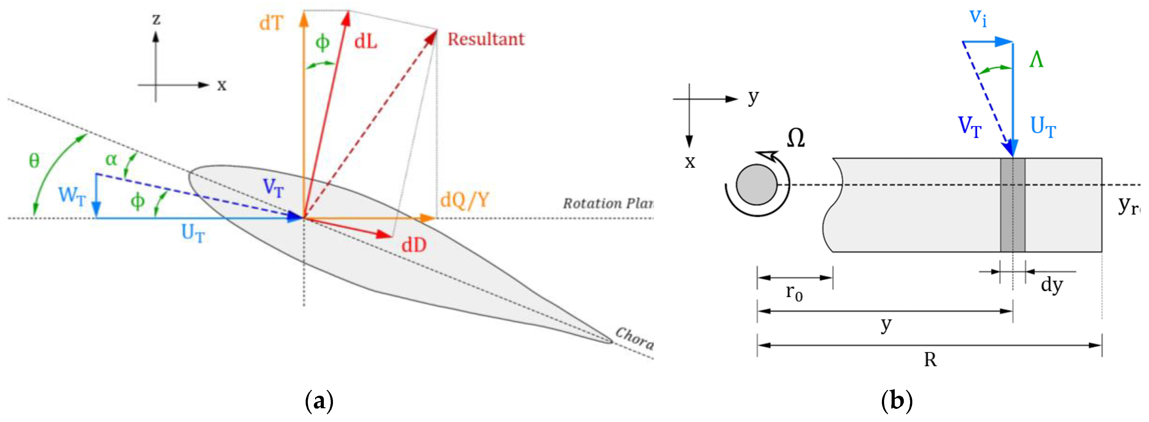
Figure 2.
Flowchart of the proprotor performance model.
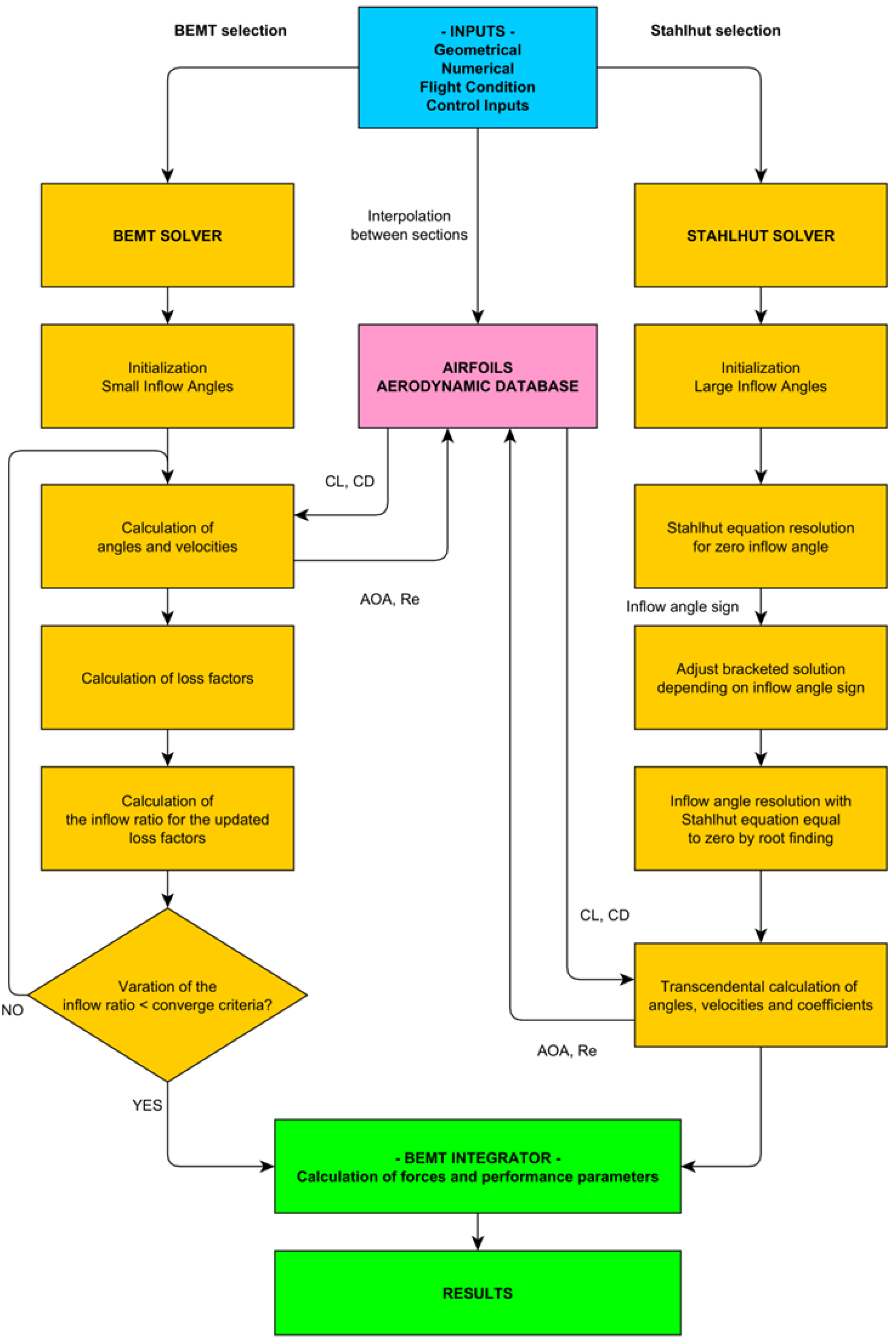
Figure 3.
Calculation of the inflow angle by the bisection method for a particular blade element.
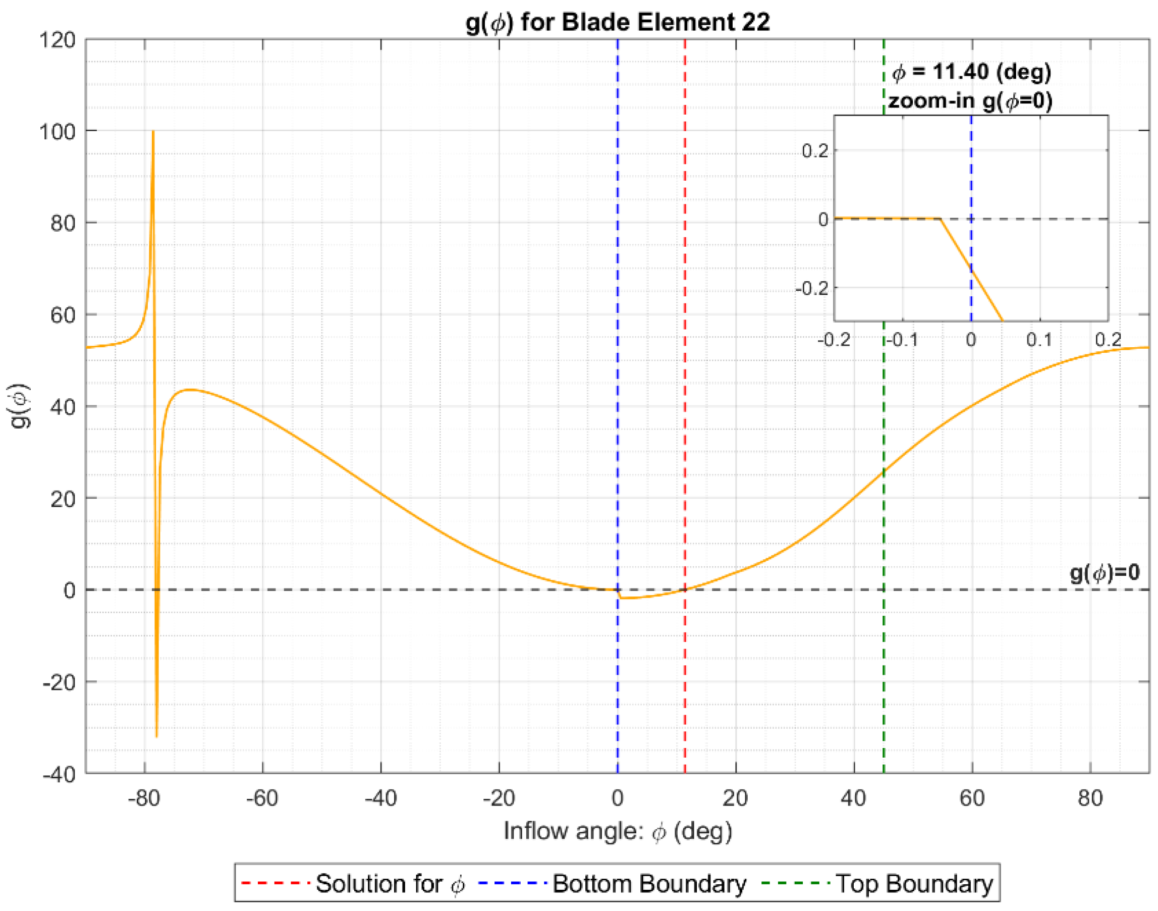
Figure 4.
Geometric twist and chord of the blade.
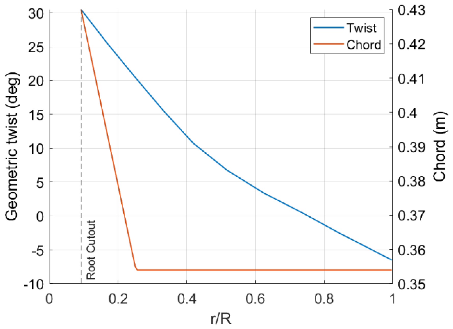
Figure 5.
Blade’s airfoil representation.
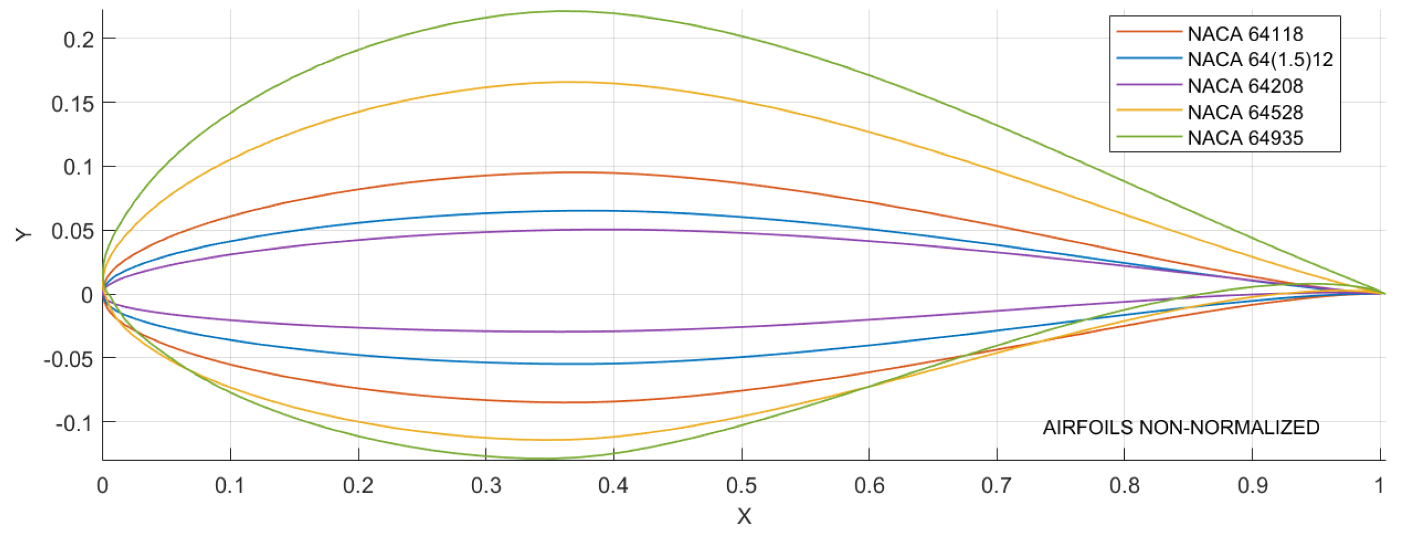
Figure 6.
Model and experimental CT versus CP absolute (a) and deviation (b) results for the Stahlhut solver and RPM = 586.
Figure 6.
Model and experimental CT versus CP absolute (a) and deviation (b) results for the Stahlhut solver and RPM = 586.
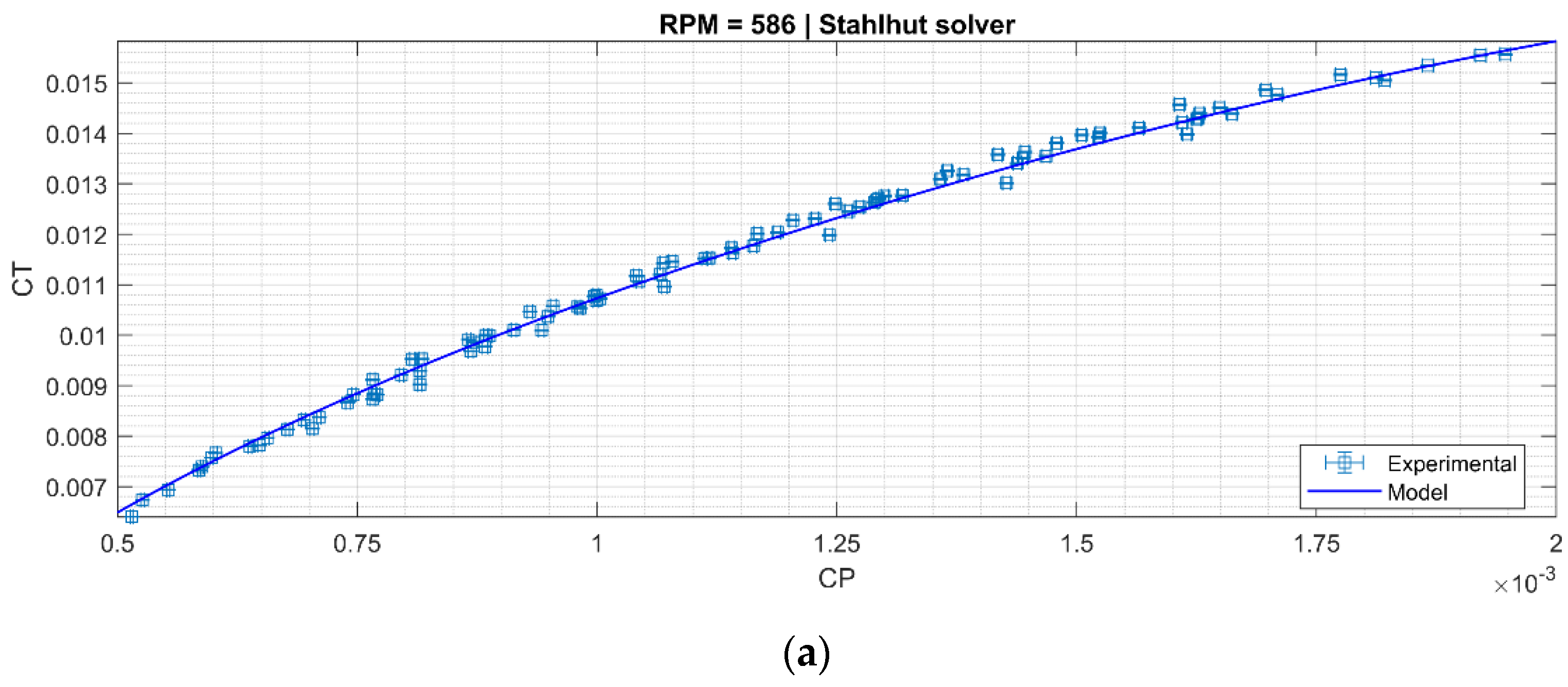
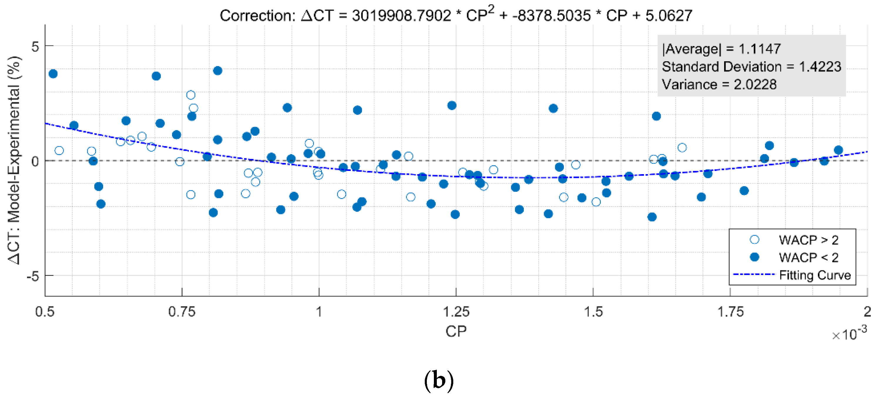
Figure 7.
PDD compilation between the model and experimental results for the BEMT (a) and Stahlhut (b) solvers.
Figure 7.
PDD compilation between the model and experimental results for the BEMT (a) and Stahlhut (b) solvers.
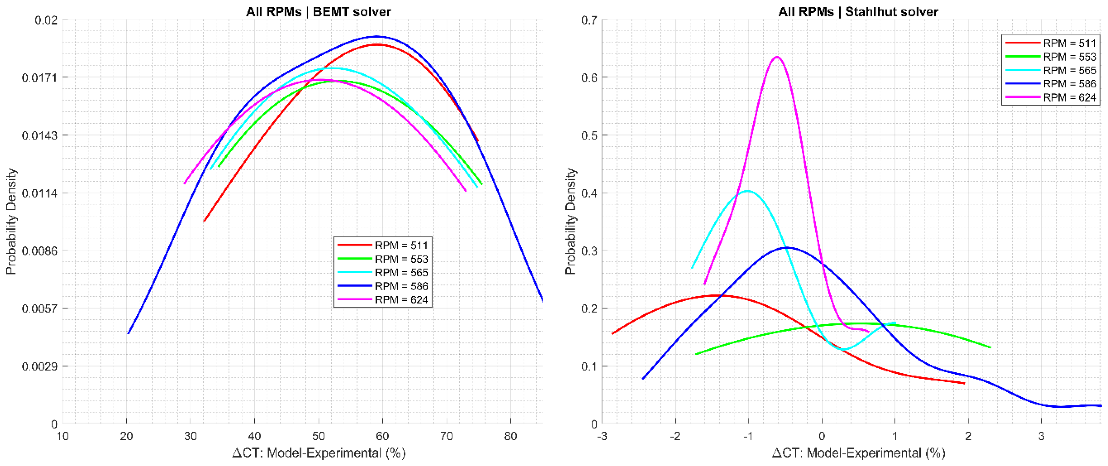

Table 1.
This is a table. Tables should be placed in the main text near to the first time they are cited.
Table 1.
This is a table. Tables should be placed in the main text near to the first time they are cited.
| Airfoil | r/R |
|---|---|
| NACA 64118 | 1.00 |
| NACA 64(1.5)12 | 0.80 |
| NACA 64208 | 0.51 |
| NACA 64528 | 0.17 |
| NACA 64935 | 0.09 |
Table 2.
Main statistical parameters from the deviation in thrust coefficient versus power coefficient.
Table 2.
Main statistical parameters from the deviation in thrust coefficient versus power coefficient.
| Solver | RPM | Samples | |Average| | Standard Deviation | Variance |
|---|---|---|---|---|---|
| BEMT | 511 | 7 | 56.07 | 15.95 | 254.44 |
| 553 | 4 | 54.40 | 14.74 | 314.73 | |
| 565 | 4 | 53.44 | 17.59 | 309.43 | |
| 586 | 168 | 54.28 | 16.33 | 266.58 | |
| 624 | 8 | 50.74 | 16.67 | 277.97 | |
| Stahlhut | 511 | 7 | 1.64 | 1.71 | 2.92 |
| 553 | 4 | 1.35 | 1.74 | 3.03 | |
| 565 | 4 | 1.12 | 1.17 | 1.38 | |
| 586 | 168 | 1.11 | 1.42 | 2.02 | |
| 624 | 8 | 0.77 | 0.68 | 0.46 |
Disclaimer/Publisher’s Note: The statements, opinions and data contained in all publications are solely those of the individual author(s) and contributor(s) and not of MDPI and/or the editor(s). MDPI and/or the editor(s) disclaim responsibility for any injury to people or property resulting from any ideas, methods, instructions or products referred to in the content. |
© 2024 by the authors. Licensee MDPI, Basel, Switzerland. This article is an open access article distributed under the terms and conditions of the Creative Commons Attribution (CC BY) license (http://creativecommons.org/licenses/by/4.0/).
Copyright: This open access article is published under a Creative Commons CC BY 4.0 license, which permit the free download, distribution, and reuse, provided that the author and preprint are cited in any reuse.


