

Submitted:
03 June 2024
Posted:
04 June 2024
You are already at the latest version
Abstract
Spectral photon counting cone-beam CT imaging is challenged by individual pixel response behaviour, which leads to noisy projection images and subsequent image artefacts like rings. Existing methods to correct for this either use calibration measurements, like signal-to-thickness calibration (STC), or perform post-processing ring artefact correction of sinogram data or scan reconstructions, without taking the pixel response explicitly into account. Here we present a novel post-processing method (DAC-shifting), which explicitly measures the current pixel response using flat field images, and subsequently corrects the projection data. The DAC-shifting method was evaluated with a repeat series of spectral photon counting imaging (Medipix3) of a phantom with different density inserts, and in iodine K-edge imaging. The method was also compared against PMMA based STC. The DAC-shifting method was shown to be effective in correcting individual pixel response, and was robust against detector instability. On the contrary, STC correction showed varying results, which was almost as good as DAC-shifting when data was acquired just after STC calibration, but worse with larger time differences. In K-edge imaging, DAC-shifting provides a sharper attenuation peak, and more uniform CT values, which is expected to benefit iodine concentration quantification.
Keywords:
spectral CT
; K-edge imaging
; photon counting detector
; cone-beam CT
; pixel response correction
; Medipix3
1. Introduction
In the past decade, computed tomography (CT) research has been focused on replacing energy integrating detectors (EID) with energy discriminating photon counting detectors (PCD). With PCD-CT imaging, you can reach a higher spatial resolution, signal-to-noise ratio, and contrast-to-noise ratio compared to EID-CT ([1]). Furthermore, the energy discriminating ability allows you to acquire several energy bins during a scan, which allows for material decomposition, for example fat, water, and lipid concentrations ([2]), or to distinguish multiple contrast agents ([3]).
PCDs typically consist of multiple chips which each have a two-dimensional readout grid (application specific integrated circuit, ASIC) coupled to a semiconductor such as cadmium telluride (CdTe) or silicon (Si) which generates an electrical charge. The energy discrimination is implemented by thresholding the electrical charges using two or more counters. For normal operation, the first counter is set above the electrical noise of the system. Subsequent counters can be set to energy specific values, making sure that the electrical charge created by a photon is counted only when it exceeds the threshold value. One example of a PCD chip is the Medipix3RX, which consists of 256 × 256 pixels with a pixel pitch of 55 m and two threshold counters per pixel ([4]). In spectroscopic configuration, 2 × 2 pixels are combined, resulting in a 110 m pixel pitch and eight counters per pixel ([5]). The chips can be tiled together to create a large field of view (FOV). Clinical devices using this technology are the MARS Bioimaging system ([6]) and the spiral breast CT imaging system ([7])
The thresholds for the counters are set per chip and are defined as integer numbers (typical range 0 — 255 or 511), which are also known as digital-to-analogue-converter (DAC) units. The relation between DAC and actual keV threshold is close to linear and needs to be calibrated for each chip. Several methods for calibration exist, of which the following three are most common, 1) kVp scanning with a polychromatic x-ray source, where you change the DAC from high to low, searching for the setting where a pixel starts to count photons, which corresponds to the kVp ([8]); 2) x-ray fluorescence (XRF) of pure metal foils, where you search for the DAC corresponding to the characteristic K-shell electron transition energies of the metals ([8]); 3) use of monochromatic/radioactive x-ray sources, where the highest DAC with substantial counts corresponds to the source energy. With two or ideally more points within the energy range of interest, the linear relation can be determined.
While DAC settings are set per chip, the actual response varies per pixel. This means that on average, the image acquired with a certain threshold corresponds to a specific keV value, but the image will be noisy, because individual pixels represent a specific range of keV threshold values. These pixel-response variations result in ring artefacts in the reconstructed images, and therefore, projection images need to be corrected first. Basic flat field correction (FFC) is not sufficient, because the count response of the pixels is energy and flux dependent, and because of beam hardening that is present in the projection images.
One well known method to correct for the individual pixel response is the so-called signal-to-equivalent thickness calibration method (STC) ([9,10,11]). In STC, a set of homogeneous flat absorbers (for example sheets of aluminium or PMMA) are imaged with a PCD, with a fixed set of thresholds and x-ray tube settings. The non-linear relationship between absorber thickness and photon counts is subsequently fitted per pixel. To apply the STC method on imaging data of samples, you replace the counts in the projection images with the corresponding thickness. This method has the advantage that it corrects both for pixel response, and for beam-hardening. As the STC method is based on calibration data, it is highly dependent on stability of the imaging system, including the x-ray source and the detector response.
Alternative methods focus on removal of the ring artefacts either by correcting the sinogram data or the reconstructed image ([12]). Especially corrections on the sinogram data have shown to do a respectable job on removing the ring artefacts, but challenges can be present at high contrast edges, and with small objects or particles within the scanned object.
The above-described methods are mostly focused on correcting data, which is non-spectral, like with EID scans, or on correcting individual spectral threshold/bin data from PCDs. The corrections methods do not explicitly incorporate individual pixel spectral response, which is the cause of the problem in the first place. When PCDs are used to acquire multi-spectral data, with more than two thresholds, there is a risk that individual threshold correction can lead to corruption of the spectral integrity of the data.
In this work, we introduce an image post-processing method that does not require predefined calibration images. Instead, we used flat field images, acquired just before or after scan acquisition of a sample, to determine the individual pixel response in terms of DAC-to-keV at the time of scanning. In the next step, the spectral projection data was fitted per pixel and per projection using cubic-B-splines, and the counts for each pixel were corrected per keV threshold using the individual pixel response. With this method we assumed that the x-ray source and detector response was stable within the scan acquisition, while we mitigate fluctuations over longer time periods. The method allows for freedom in choosing the x-ray source settings, and the number and level of thresholds.
The purpose of this study was to describe the method, illustrate its performance, and compare the resulting reconstruction image quality with standard flat field correction, and PMMA based STC. For this purpose, we used a custom phantom with different plastics, water, and oil, and performed K-edge imaging of a phantom containing different concentrations of iodine.
2. Materials and Methods
2.1. Experimental Setup
A schematic view of the experimental setup is shown in Figure 1. A radiation shielded X-ray cabinet (EZ-Access, Metrix NDT Ltd, Loughborough, U.K.) was used, equipped with a static microfocus X-ray source with a focal spot of 5—7 m (L9421-02, Hamamatsu Photonics K.K, Hamamatsu, Japan), a sample stage with four degrees of freedom (X, Y, Z, R), and a detector stage with three degrees of freedom (X, Y, Z). A 500 m thick aluminium filter is used for all measurements to reduce the proportion of low energy photons.
For imaging, we used two Medipix3 detectors from two different manufacturers. The first was an air-cooled 2 × 2 grid layout detector with 500 m silicon (Si) sensor material biased to +150 V (Amsterdam Scientific Instruments B. V., Amsterdam, the Netherlands). The second detector had a 2 × 5 layout, water-cooling, also a 500 m Si sensor material, and the bias voltage was +150 V (WidePIX, Advacam S.R.O., Prague, Czech Republic). Both detectors have a pixel pitch of 55 m , with chips of 256 × 256, and two energy thresholds. Each chip of each detector was first calibrated using XRF measurements using pure metal foils of Cu (8.0 keV), Mo (17.4 keV), Rh (20.1 keV), and Sn (25.1 keV) ([8]);
Imaging of samples was done using step-and-shoot, meaning that the sample stage was static during acquisition of projection data. To acquire spectral data with only two thresholds per chip, we acquired multiple projection images at each rotation angle of the sample, where the thresholds in keV were changed for each projection. Before and after acquisition of projection data a set of ten open images with the same threshold settings was acquired.
2.2. Image Post-Processing (DAC-Shifting)
Our proposed image post-processing method, called DAC-shifting, consists of two major steps, see Figure 2. In step 1, the individual pixel response was modelled using the flat field data. Here we assumed an ideal setup, where the x-ray spectrum and flux are homogeneous over the entire detector. We also assumed that the XRF chip calibration assures that image acquisition with a certain threshold in keV results in comparable photon counts between the chips. With these assumptions, the ideal flat field image is a homogeneous image with a certain amount of photon counts for each threshold. For each specific threshold, the median number of photon-counts over the entire image was taken as ideal target counts per threshold. Subsequently, the individual pixel response was modelled using cubic b-spline fits through the different flat field thresholds, using the chip DAC units on the x-axis, and the pixel specific counts on the y-axis. The individual pixel fits were then used to find which DAC setting per threshold corresponds to the ideal target count. The prime outcome of this step was a look-up-table (LUT) that describes for every individual pixel which DAC unit corresponds to which keV threshold.
In step 2, the projection data was processed and corrected. For each projection angle the individual pixel data was fitted using a cubic b-spline, again using the chip DAC units of the different thresholds on the x-axis, and the pixel specific counts on the y-axis. With the LUT from step 1, the counts in each pixel and threshold were then corrected such that every pixel reflects the same keV threshold. As a result, all the projection data was corrected using the individual spectral response of the pixels. For FFC in the image reconstruction part, the ideal median counts per threshold were used instead of the actual flat fields.
It is important to note that the DAC-shifting method was performed separately for each counter. This was needed because the individual pixel response was also counter specific.
2.3. Phantom Imaging
To match the size of the detector, a small custom phantom was produced. It is a 20.0 mm diameter cylinder with a lid, both made of PMMA-c. It has seven 4.0 mm diameter holes along the length of the cylinder which hold other materials. These materials were water, sunflower-oil, PC, PEEK, POM-c, and PTFE, and centrally air, and were chosen due to their relatively similar X-ray attenuation coefficients and densities.
The phantom was imaged with both detectors, with a distance-source-detector (DSD) of 171 mm, and distance-source-object (DSO) of 123 mm. In total, 720 projections angles (0.5 degree spacing) were acquired, with for each angle five acquisitions using both threshold counters, resulting in ten threshold projections per angle in total. Exposure time per threshold was optimised to achieve similar counts for the different thresholds (Table 1).
The x-ray source was set to 50 kVp and 160 A. In each imaging session, the phantom was scanned twice. First using a static detector position, followed by an acquisition with random detector shifts between -5 and +5 pixels in the x- and y-direction, similar to ([13]). The random detector shifts were used as hardware solution to mitigate ring artefacts, which comes at the cost of more noise in the reconstructed image. For comparison between both PCDs, only data of four of the ten chips in the WidePIX detector were used. For one detector, these measurements were performed three times in a time span of 25 days. This was done to showcase the stability of the system. An overview of the measurements taken can be found in Table 2.
For image analysis, materials were segmented out using combinations of circular masks defined by centres and radii, see Figure 3. A margin (black border) was used around each selection because the materials were not perfect cylinders due to the manufacturing method and the cylinders were not perfectly aligned in the Z axis.
For the sake of illustration, Figure 4 shows an example of a CT reconstruction in all three spatial planes. The example reconstructed slice shown throughout this work was fixed at the same XY plane. This was chosen as it is a good representation of an average slice. It also contains two distinct relatively high attenuation dots of a few pixels in size in the lower right quadrant, on the edge of the PC (polycarbonate). These can be used to visually assess the reconstructed image quality. The viewing window is fixed at -1000 — 1800 HU for all slice plots, unless otherwise stated.
2.4. Image Reconstruction
For image reconstruction we used the TIGRE toolbox ([14]). Scans were reconstructed per threshold, meaning that each reconstruction represented the counts above a certain energy threshold, not an energy bin. For reconstruction we used the standard FDK (Feldkamp, Davis and Kress) option with a cosine filter. We also employed iterative FISTA (fast iterative shrinkage thresholding algorithm) reconstruction, using the FDK as prior, 100 reconstruction iterations, a hyper parameter of , and 75 denoise iterations (‘tviter’) in every reconstruction iteration. For other parameters, the defaults were used. The chosen parameters were empirically optimised to balance the trade-off between image-sharpness and noise. All reconstructions were , with isotropic voxels of 42 m.
We applied five different post-processing methods on the projection data before reconstruction. The first was standard FFC. The second method was detector based STC conversion of the counts to equivalent thicknesses of PMMA, STC-D. For STC calibration we acquired five projection images per threshold using the following thicknesses of PMMA: 0, 0.8, 1.6, 3.0, 6.0, 9.0, 12.0, 15.0, 18.0, 21.0, 24.0, 27.0, and 30.0 mm. The median number of photon-counts over the five projections for each thickness was divided by the median counts measured at thickness 0. We subsequently modelled the individual pixel response using the global hyperbolic interpolation method from [15]. For STC-D, one STC calibration curve was fitted for every threshold, using the medians of the detector. This reconstruction step corrected for beam-hardening, but not pixel response variation. The third method was individual pixel STC conversions, where calibration curves were fitted for each pixel separately, STC-P. This reconstruction step was aimed at correcting both for beam hardening and pixel response. As fourth, the DAC-shifting method was applied to correct for the pixel response only (DAC-shifting). In a last step, the STC-D and DAC-shifting were combined to correct for beam hardening and pixel response (DAC and STC). With five post-processing options, and two reconstruction methods, each projection set was reconstructed ten times.
The imaging data of the phantom was converted to Hounsfield units (HU). HU calibration for EIDs is relatively straightforward, but this is not the case for spectral data. For PCDs with configurable energy thresholds, the HU can change with respect to the energy threshold. We chose to use the median water and air values for each energy threshold as calibration reference points. The calibration becomes:
Where are linear attenuation coefficients and E is the energy at which the threshold of the detector is set to. With this approach, the median water and air HU values for each threshold are fixed to 0 and -1000, respectively. This was done for every reconstruction independently.
2.5. Statistics
In this study, we compared the effect of five different options to improve image quality: reconstruction type, DAC-shifting, STC-D, STC-P, and detector motion. For presentation of the image quality, and spectral differences between the materials, the median HU over threshold was plotted, together with the 95th percentile range of HU values present in the respective materials. For this step, cylindrical regions of interest were used, see Figure 3. The first image quality metric was the range of values for a single material within a reconstruction. We arbitrarily chose the 95th percentile range in HU and calculated the absolute difference between the upper and lower value as the percentile size. The percentile size quantifies the precision of the system; the closer to zero it is, the better. To represent the spectral information for each material, we took the median over the different thresholds for each material within a reconstruction. To represent the overall image quality for a reconstruction, the mean percentile size over the different materials was used.
To rank the impact of each option, we evaluated their effectiveness in improving the image quality. To do so, we calculated and compared the mean relative change in percentile sizes of the reconstructions along with the interquartile ranges between each pair, without and with each parameter. These data will be named ‘effectiveness score’ in this paper and will be shown in units of percentage. For example, all FDK reconstructions versus all FISTA reconstructions. Negative values show a reduction (improvement) in percentile sizes.
In addition to this, we calculated p-values using a t-test on two related samples (without and with each parameter) to quantify the similarity of the pairs to each other. ‘This is a test for the null hypothesis that two related or repeated samples have identical average (expected) values’ [16]. A p-value below 0.01 was deemed significant.
2.6. Spectral K-Edge Experiment with an Iodine Solution
This part aimed to illustrate the capability of DAC-shifting method to enhance the spectral profile (the attenuation coefficient () as a function of energy (keV)) of the iodine K-edge (33.2 keV) in both 2D and 3D spectral CT imaging.
The first experiment utilised 2D spectral imaging to examine a 3D printed cuboid vessel made of polylactic acid (PLA) with a uniform cavity thickness of 6.5 mm, containing the iodine solution at a concentration of 270 mg Iodine/ml in water (Visipaque ™, Iodixanol, GE Healthcare, Finland). This setup allowed for consistent path length measurements of the iodine solution for each pixel of the detector, employing chips. Imaging was performed using the X-ray source set at 90 kVp and 89 A, with energy thresholds ranging from 8.0 to 56.0 keV in 0.5 keV increments, each with a total exposure duration of 48 seconds. A flat field correction was applied by scanning the same cuboid vessel in an empty state under identical parameters, enabling isolated assessment of iodine solution attenuation. Additionally, flat field images were used to construct a LUT essential for the initial DAC-shifting step. The outcome of this experiment focused on the effect of DAC-shifting on the spectral profile at the entire detector matrix, each discrete chip, and individual pixels.
In the subsequent experiment, a 3D-printed (polylactic acid) cylindrical phantom with a 20.0 mm diameter was utilised to perform 3D spectral CT imaging. This phantom, with nine cylindrical cavities each 4.0 mm in diameter, was filled with varying iodine concentrations (135.0, 67.50, 33.75, 16.88, and 8.45 mg/ml), water, and three empty cavities. Guided by the spectral profile of the iodine solution established in the 2D spectral imaging experiment, thresholds were selected for 3D spectral CT acquisition as presented in Table 3, specifically targeting the iodine K-edge.
The phantom was imaged with the following system configuration with detector motion and using the step-and-shoot acquisition mode:
- Tube voltage = 90 kVp
- Tube current = 89 A
- DSO (distance source object distance) = 123.0 mm
- DSD (distance source detector) = 163.0 mm
- Projections = 720
- Rotation angle =
- Reconstructed voxel size = 0.0415
Ten flat field images were acquired before and after the projection images. CT reconstructions were then performed as described in Section 2.4 using both reconstruction algorithms, without and with DAC-shifting. Cylindrical regions of interest (volume = 79 ) as shown in Figure 5 were used to evaluate each iodine concentration.
The quantification of different iodine concentrations was achieved by examining the Hounsfield units at 33.0 keV, the energy level closest to the K-edge peak. A linear regression model () was used to evaluate the correlation between iodine concentrations and CT numbers. The y-intercept was set to the HU of water (zero). Further, the values of without and with DAC-shifting methods at 33.0 keV were compared using Fisher’s r-to-z transformation, calculating the z-score and corresponding p-value to determine the significance of the difference between the two correlation coefficients.
3. Results
3.1. Out-of-the-Box Imaging
To set the reference, we start with a CT reconstruction showing the out-of-the-box (OOTB) experience (upper row of Figure 6). Apart from manufacturer specific procedures, the only calibration done at this stage was a basic energy calibration per chip using XRF. This only ensured that the chips were aligned in terms of energy to first order.
The spectral profile of the different materials can be seen in Figure 7. Note that despite the increasing exposure time used for increasing thresholds, there was a substantial increase in percentile size with increasing thresholds. Also note that the 95th percentile bands overlap each other for most materials.
3.2. Effectiveness Scores
In Table 4 an overview of the effectiveness scores for the investigated options on the different datasets can be seen. In the following sections each option is separately illustrated.
3.3. STC-D Beam Hardening Correction and Detector Motion
The effect of the STC-D beam hardening correction is visualised in Figure 6. From the profile lines in the figure, especially at the 5 keV threshold, clearly there was beam hardening present in OOTB, which was corrected using STC-D. The overall effect of STC-D on the effectiveness score was limited (Table 4), as the beam hardening was present mainly in the PMMA bulk and the PTFE, but not in the other materials.
The detector motion method effectively translated the ring artefacts caused by pixel response differences into random appearing noise in the reconstructions (Figure 8). As the method changes the appearance of the image, but not the value range within the materials, the mean percentile sizes were not substantially affected most of the time (Figure 9). The combined effectiveness score for detector motion limited to -8.7 % (IQR -13.0 — -1.5 %), .
3.4. STC-P Beam Hardening and Pixel Response Correction
We observed substantial differences in the effectiveness of STC-P with the different datasets (Figure 10). The effect of STC-P on two different datasets is visualised in Figure 11. The corresponding effectiveness scores varied in range from -10.0 — -43.7 % for the ASI data, and even a worse image quality for the ADVACAM-1 data (effectiveness score +45.5 % (+39.2 : +52.3), Table 4). The two datasets that were acquired close to the date of acquiring the STC-D calibration measurements (ASI-2 and ASI-3) seemed to benefit more from STC-D than the other datasets.
3.5. DAC-Shifting
The DAC-shifting method was focused on correcting the individual pixel response, using a LUT based on the flat field images of the day. An example of a LUT for a specific threshold and its variation over different datasets can be seen in Figure 12. In this example, the 95 % range of DAC settings for individual pixels that correspond to 14 keV stretches from 73 — 105 DAC units. The stability over different datasets seems random and the root-mean-square (RMS) standard deviation of Figure 12 c corresponds to 2.33 DAC units, which typically corresponds to 0.47 keV.
In Figure 13, we illustrated the effect of DAC-shifting in projections and sinograms at two thresholds and compared it to STC-P. Note the significant reduction in vertical stripes in the sinogram images, especially at the higher threshold. In addition, individual chips can be distinguished in the OOTB and STC-P projections, but not in the DAC-shifting projections.
With DAC-shifting, ring artefacts were substantially reduced, without degradation of spatial resolution or introduction of obvious artefacts (Figure 14). DAC-shifting also resulted in comparable image quality between different datasets (Figure 15). The absolute mean percentile sizes with DAC-shifting are comparable between the datasets, even when the absolute numbers without DAC-shifting vary (for example, ASI-1 vs. ASI-3). As a result, the effectiveness scores were substantial (mean -47.4 %) and varying based on the initial image quality (-40.7 — -55.6 %), .
3.6. Reconstruction Methods
So far, we have visualised reconstructions using only the FDK method. The comparison between the iterative reconstruction algorithm, FISTA, and FDK is shown in Figure 16. The FISTA method as used in this work was very effective in reducing the noise in the image, with minimal compromise for the image sharpness. The noise reduction clearly translated into reduced mean percentile differences. As a result, the effectiveness score was -61.6 % (IQR -66.0 — -59.1 %), .
3.7. Optimal Settings
The best combination of options was detector motion, STC-D, DAC-shifting, and FISTA reconstruction. Even though the effectiveness score for detector motion was close to zero, it complements the FISTA reconstruction. This is because detector motion smears the rings into noise, which can effectively be reduced by the FISTA reconstruction. An illustration of the image improvement compared to the out-of-the-box setting using FISTA can be seen in Figure 17. The spectral data of the best parameter combination can be seen in Figure 18.
3.8. Evaluation of DAC Shifting - Iodine K-Edge Imaging
The capability of the DAC-shifting method to enhance the sharpness of the iodine K-edge using 2D spectral imaging is illustrated in Figure 19. The spectral profiles show that attenuation increases as the energy approaches the K-edge and decreases after passing it. Without DAC-shifting, individual pixel response variations led to a relatively wide 95 % data range. In contrast, the DAC-shifting method improved homogeneity between individual chips (see attenuation images) and pixels (see 95 % data range), resulting in a sharper attenuation peak near the K-edge.
In 3D spectral iodine imaging, the spectral profiles, depicted in CT number (HU) as a function of energy, still show increased CT numbers around the K-edge, but less pronounced than in the 2D imaging (Figure 20). Note that the highest concentration in the 3D imaging was half of the concentration in the 2D imaging. The effect of DAC-shifting was again mainly visible in a reduction of the 95 % data range, especially at the higher thresholds. This resulted in less overlap between the 95 % data ranges in the lower iodine concentrations, as can be appreciated from the linear relationships depicted in Figure 20 Comparison of values demonstrating a highly significant difference (p <0.001) between without DAC-shifting and with DAC-shifting methods.
4. Discussion
In this paper, we presented a novel post-processing method to deal with individual pixel response in spectral imaging with PCDs. We have shown how the DAC-shifting method has a positive impact on the image quality, also in relation to existing methods. We have also shown that DAC-shifting is robust against long term variations in the imaging system, while STC-P did not provide consistent image-quality improvements over time.
When comparing the DAC-shifting method with the STC-P method, we can see that at best, with the most optimal settings, they perform almost comparably. In the ASI datasets with motion, the mean percentile sizes for STC-P with FISTA were 68, 57 and 53 HU for ASI-1, ASI-2 and ASI-3, respectively (Figure 10). For DAC-shifting in combination with STC-D and FISTA reconstruction, the mean percentile sizes were 50, 50 and 49 HU (Figure 15). In general, the results on DAC-shifting were very stable when comparing the effect of the different post-processing methods on the different datasets, even when comparing the two detectors (Figure 15). For STC-P, the changes in mean percentile size were much less stable, and it appears that it only worked for ASI-2 and ASI-3, which were acquired within four days of the STC calibration measurements. These findings exemplify the instability of this imaging system, this is observed in previous work using a Medipix3 based system [17]. This instability was further illustrated and quantified in the LUT variation example in Figure 12 where the RMS of the standard deviation map was 2.33 DAC units, which corresponds to a 0.47 keV standard deviation in this system. In other words, within the data acquired in a four week window, individual pixel responses at 14.0 keV can vary between -1.0 — +1.0 keV. Given the random distribution of the variation in the example image, the variation can be attributed to the detector, not the x-ray source.
Even though several papers are available on STC-P, none of them describe the relation between system stability and effectiveness ([9,10,11,15]). This makes a direct comparison to other papers challenging. The most comparable work in terms of imaging with Medipix3 and low threshold energies is the work by Ronaldsen et al. using the MARS-CT scanner in 2012 [2]. The spectral profile on sunflower oil obtained in our work (Figure 18) seems directly comparable to their work, with slowly increasing CT numbers above 15 keV threshold. Unfortunately, they only mention a standard deviation uncertainty of ~10 HU, without explicitly showing the data. They make use of a combined wavelet-Fourier filtering method for ring artefact correction [18], but the effect of this is not separately illustrated. They also imaged iodine, at a concentration of 0.01 mol/l, lower than our lowest concentration (0.033 mol/l). However, they only measured thresholds of 30.9 and 36.2 keV around the K-edge, for which the K-edge was not directly visualised.
He et al. performed more comparable K-edge imaging of iodine, both in 2D and 3D [6]. They showed similar graphs regarding the K-edge in terms of attenuation over energy (Figure 19). In their and our work, the ability to precisely resolve the K-edge is limited by the effective spectral resolution of the detector. The spectral profile appears to be between the theoretical mass attenuation example with a 1.0 and 3.0 keV (energy resolutions) provided by Ge et al. [6]. In their example, they show that a limited energy resolution convoluted with the sharp K-edge, which shifts the attenuation peak to a slightly higher energy.
When calibrating the Medipix3 detector, an equalisation procedure minimises the variation in pixel response at a specific threshold. In our setup, we focus our research on low keV thresholds. The Advacam detector was equalised at approximately 8.0 keV, whereas the ASI detector was configured using the noise edge, which is approximately 4.0 keV. Due to threshold dispersion, where the pixel responses diverge as the threshold is increased, the DAC-shifting improvement was more significant at the higher thresholds, achieving comparable image quality between 5.0 and 20.0 keV (Figure 17). Alternative methods, like loading specific equalisation maps for each threshold used could help increase the image quality of the raw data. Currently, this step would increase the acquisition time substantially, as loading of the equalisation maps takes time.
Due to the instability of our imaging system, the STC-P method did not provide consistent image quality improvement. To make use of the advantage of STC in correcting for beam-hardening, we introduced the STC-D method. To the best of our knowledge, this approach was not used before. In our setting, the advantage was that STC-D can be combined with the DAC-shifting method. The method is simple, reliable and fast, because it can be applied to the entire stack of projection data at once and is less sensitive to variations over time. Of course, the effectiveness of STC-D beam hardening correction is dependent on the materials used for calibration, PMMA in our case, and the sample that is imaged. For the phantom with plastic inserts it worked well, but for the iodine acquisitions, it showed less effective (data not shown), this was at least partly due to the minimal beam hardening at the higher energies.
In recent years, there has been focus on improving spectral image quality by utilising dedicated spectral reconstruction methods with material decomposition [19,20,21], and deep-learning based reconstruction for noise reduction [22,23], or combinations thereof [24]. While these novel methods all seem very promising, they could still use the advantage of the presented DAC-shifting method. The method corrects the projection data, keeping the spectral integrity, without changing the units, and homogenises data between the different chips and pixels. In this way, the input data for reconstruction is improved, providing improvements for downstream steps like material decomposition. The challenge of our method is that it adds measurement and processing time. It took between 10 and 12 minutes to apply DAC-shifting on a modern 64 core computer (AMD Ryzen Threadripper 3990X) utilising Python and parallel processing on 60 of the cores for most of the steps. To speed this up, there are many options. One of which is a neural network for the DAC-shifting method to improve processing speed.
The presented DAC-shifting method has some limitations. First of all, the method is based on performing cubic b-spline fits through the spectral data, which means that it can only be used on spectral data, and not for individual single-threshold data. The cubic b-spline approach does not utilise any knowledge about the underlying physics. Ideally we would fit a function which is related to the underlying physics with a data based uncertainty estimation to constrain the fits. Secondly, at the edges of the spectral data, the lowest and highest threshold, approximately half of the pixels were corrected using extrapolation of the data, which is less accurate than interpolation due to the cubic b-spline approach. This effect was visible in Figure 18, where the 95 % data range increased at the highest threshold plotted. Note that in our work we already used one extra threshold acquisition (Table 1 , threshold 0 = 25.0 keV; threshold 1 = 30.0 keV), to mitigate this issue. This data was only used to guide the spline fitting, but the DAC-shifted reconstructions with these thresholds did not result in improved image quality. This is due to the extrapolation (data not shown). Thirdly, since each counter corresponds to different transistors, and therefore each counter has their individual response patterns, the DAC-shifting method was applied per counter. This means that the approach is currently not applicable to PCDs that have many more counters per pixel where the entire spectral profile can be acquired at once. Further research is needed to address application in these detectors, a first approach was taken in [17]. Finally, we reconstructed our data as spectral thresholds, not spectral bands (energy bins), which are often presented in other papers. However, the DAC-shifting method is applicable in both cases. When spectral bands are needed, the DAC-shifting method can be applied first on the threshold data, and subsequently spectral bands can be calculated by subtracting two thresholds.
5. Conclusions
Within the context of improving reconstruction quality of our system, we have presented a novel post-processing method that minimises individual pixel response in spectral photon counting cone-beam CT. The method was shown to be consistently effective in correcting the sinogram data, which resulted in reduced ring artefacts and improved image quality. This was supported with the iodine concentration measurements. It does not appear to introduce artefacts and maintains the scale and units of the data. DAC-shifting was also shown to provide consistent image quality, even with variable quality input data.
Author Contributions
The author’s initials will be used for the sake of brevity. Conceptualisation, JN, NJSB and ICR; methodology, JN, NJSB and ICR; software, JN, NJSB and ICR; validation, all authors; formal analysis, JN, NJSB and ICR; investigation, JN, NJSB and ICR; resources, JN, NJSB and ICR; data curation, JN, NJSB and ICR; writing—original draft preparation, JN, NJSB and ICR; writing—review and editing, all authors; visualisation, JN, NJSB and ICR; supervision, JN, NJSB and TT; project administration, NJSB and JN; funding acquisition, JN and TT. All authors have read and agreed to the published version of the manuscript.
Funding
This research was funded by Novo Nordisk Foundation grant number NNF195A0059372, Danish Cancer Society grant number R279-A16481, and Aarhus University Research Foundation grant number AUFF-E-2021-9-15.
Institutional Review Board Statement
Not applicable.
Data Availability Statement
Imaging data that was used in this study can be shared upon request.
Conflicts of Interest
The authors declare no conflicts of interest.
References
- Wu, Y.; Ye, Z.; Chen, J.; Deng, L.; Song, B. Photon Counting CT: Technical Principles, Clinical Applications, and Future Prospects. Academic radiology 2023, 30, 2362–2382. [Google Scholar] [CrossRef] [PubMed]
- Ronaldson, J.P.; Zainon, R.; Scott, N.J.A.; Gieseg, S.P.; Butler, A.P.; Butler, P.H.; Anderson, N.G. Toward quantifying the composition of soft tissues by spectral CT with Medipix3. Medical physics 2012, 39, 6847–6857. [Google Scholar] [CrossRef] [PubMed]
- Si-Mohamed, S.; Tatard-Leitman, V.; Laugerette, A.; Sigovan, M.; Pfeiffer, D.; Rummeny, E.J.; Coulon, P.; Yagil, Y.; Douek, P.; Boussel, L.; Noël, P.B. Spectral Photon-Counting Computed Tomography (SPCCT): in-vivo single-acquisition multi-phase liver imaging with a dual contrast agent protocol. Scientific Reports 2019 9:1 2019, 9, 1–8. [Google Scholar] [CrossRef] [PubMed]
- Ballabriga, R.; Alozy, J.; Blaj, G.; Campbell, M.; Fiederle, M.; Frojdh, E.; Heijne, E.H.; Llopart, X.; Pichotka, M.; Procz, S.; Tlustos, L.; Wong, W. The Medipix3RX: a high resolution, zero dead-time pixel detectorreadout chip allowing spectroscopic imaging. Journal of Instrumentation 2013, 8, C02016. [Google Scholar] [CrossRef]
- Marsh, J.F.; Jorgensen, S.M.; Rundle, D.S.; Vercnocke, A.J.; Leng, S.; Butler, P.H.; McCollough, C.H.; Ritman, E.L. Evaluation of a photon counting Medipix3RX cadmium zinc telluride spectral x-ray detector. Journal of Medical Imaging 2018, 5, 043503. [Google Scholar] [CrossRef] [PubMed]
- He, P.; Yu, H.; Thayer, P.; Jin, X.; Xu, Q.; Bennett, J.; Tappenden, R.; Wei, B.; Goldstein, A.; Renaud, P.; Butler, A.; Butler, P.; Wang, G. Preliminary experimental results from a MARS Micro-CT system. Journal of X-ray science and technology 2012, 20, 199–211. [Google Scholar] [CrossRef] [PubMed]
- Berger, N.; Marcon, M.; Frauenfelder, T.; Boss, A. Dedicated Spiral Breast Computed Tomography With a Single Photon-Counting Detector: Initial Results of the First 300 Women. Investigative radiology 2020, 55, 68–72. [Google Scholar] [CrossRef] [PubMed]
- Panta, R.K.; Walsh, M.F.; Bell, S.T.; Anderson, N.G.; Butler, A.P.; Butler, P.H. Energy calibration of the pixels of spectral X-ray detectors. IEEE Transactions on Medical Imaging 2015, 34, 697–706. [Google Scholar] [CrossRef] [PubMed]
- Juntunen, M.A.; Inkinen, S.I.; Ketola, J.H.; Kotiaho, A.; Kauppinen, M.; Winkler, A.; Nieminen, M.T. Framework for Photon Counting Quantitative Material Decomposition. IEEE Transactions on Medical Imaging 2020, 39, 35–47. [Google Scholar] [CrossRef] [PubMed]
- Persson, M.; Bornefalk, H. A Framework for evaluating threshold variation compensation methods in photon counting spectral CT. IEEE Transactions on Medical Imaging 2012, 31, 1861–1874. [Google Scholar] [CrossRef]
- Vavrik, D.; Holy, T.; Jakubek, J.; Pospisil, S.; Vykydal, Z.; Dammer, J. Direct thickness calibration: Way to radiographic study of soft tissues. <italic>Astroparticle, Particle and Space Physics, Detectors and Medical Physics Applications - Proceedings of the 9th Conference</italic> <bold>2006</bold>, pp. 773–778. [CrossRef]
- Abu Anas, E.M.; Kim, J.G.; Lee, S.Y.; Hasan, M.K. Comparison of ring artifact removal methods using flat panel detector based CT images. Biomedical engineering online 2011, 10. [Google Scholar] [CrossRef] [PubMed]
- Liu, Y.; Wei, C.; Xu, Q. Detector shifting and deep learning based ring artifact correction method for low-dose CT. Medical Physics 2023, 50, 4308–4324. [Google Scholar] [CrossRef] [PubMed]
- Biguri, A.; Dosanjh, M.; Hancock, S.; Soleimani, M. TIGRE: a MATLAB-GPU toolbox for CBCT image reconstruction. Biomedical Physics & Engineering Express 2016, 2, 055010. [Google Scholar] [CrossRef]
- Gustschin, N.; Gustschin, A.; Epple, F.M.; Allner, S.; Achterhold, K.; Herzen, J.; Pfeiffer, F. Signal-to-thickness calibration and pixel-wise interpolation for beam-hardening artefact reduction in microCT. Europhysics Letters 2019, 125, 38003. [Google Scholar] [CrossRef]
- scipy.stats.ttest_rel — SciPy v1.13.0 Manual, 2024.
- Bal, N.J.S.; Fransen, M.; Linde, F.L. Medipix3: Spectral X-ray micro-CT and hadron therapy. PhD thesis, Universiteit van Amsterdam, Amsterdam, 2023.
- Münch, B.; Trtik, P.; Marone, F.; Stampanoni, M. Stripe and ring artifact removal with combined wavelet–Fourier filtering. Optics express 2009, 17, 34–35. [Google Scholar] [CrossRef] [PubMed]
- Simard, M.; Bouchard, H. One-step iterative reconstruction approach based on eigentissue decomposition for spectral photon-counting computed tomography. Journal of medical imaging (Bellingham, Wash.) 2022, 9. [Google Scholar] [CrossRef] [PubMed]
- Rodesch, P.A.; Si-Mohamed, S.A.; Lesaint, J.; Douek, P.C.; Rit, S. Image quality improvement of a one-step spectral CT reconstruction on a prototype photon-counting scanner. Physics in medicine and biology 2023, 69. [Google Scholar] [CrossRef] [PubMed]
- Zimmerman, K.C.; Sharma, G.; Parchur, A.K.; Joshi, A.; Schmidt, T.G. Experimental investigation of neural network estimator and transfer learning techniques for K-edge spectral CT imaging. Medical physics 2020, 47, 541–551. [Google Scholar] [CrossRef] [PubMed]
- Shi, Y.; Gao, Y.; Xu, Q.; Li, Y.; Zhang, C.; Mou, X.; Liang, Z. Learned Tensor Neural Network Texture Prior for Photon-Counting CT Reconstruction. IEEE transactions on medical imaging 2024, PP, 1–1. [Google Scholar] [CrossRef] [PubMed]
- Nadkarni, R.; Clark, D.P.; Allphin, A.J.; Badea, C.T. A Deep Learning Approach for Rapid and Generalizable Denoising of Photon-Counting Micro-CT Images. Tomography (Ann Arbor, Mich.) 2023, 9, 1286–1302. [Google Scholar] [CrossRef]
- Di Trapani, V.; Brombal, L.; Brun, F. Multi-material spectral photon-counting micro-CT with minimum residual decomposition and self-supervised deep denoising. Optics express 2022, 30, 42995. [Google Scholar] [CrossRef]
Figure 1.
Schematic overview of the experimental setup from the top view, with the coordinate system shown on the right.
Figure 1.
Schematic overview of the experimental setup from the top view, with the coordinate system shown on the right.
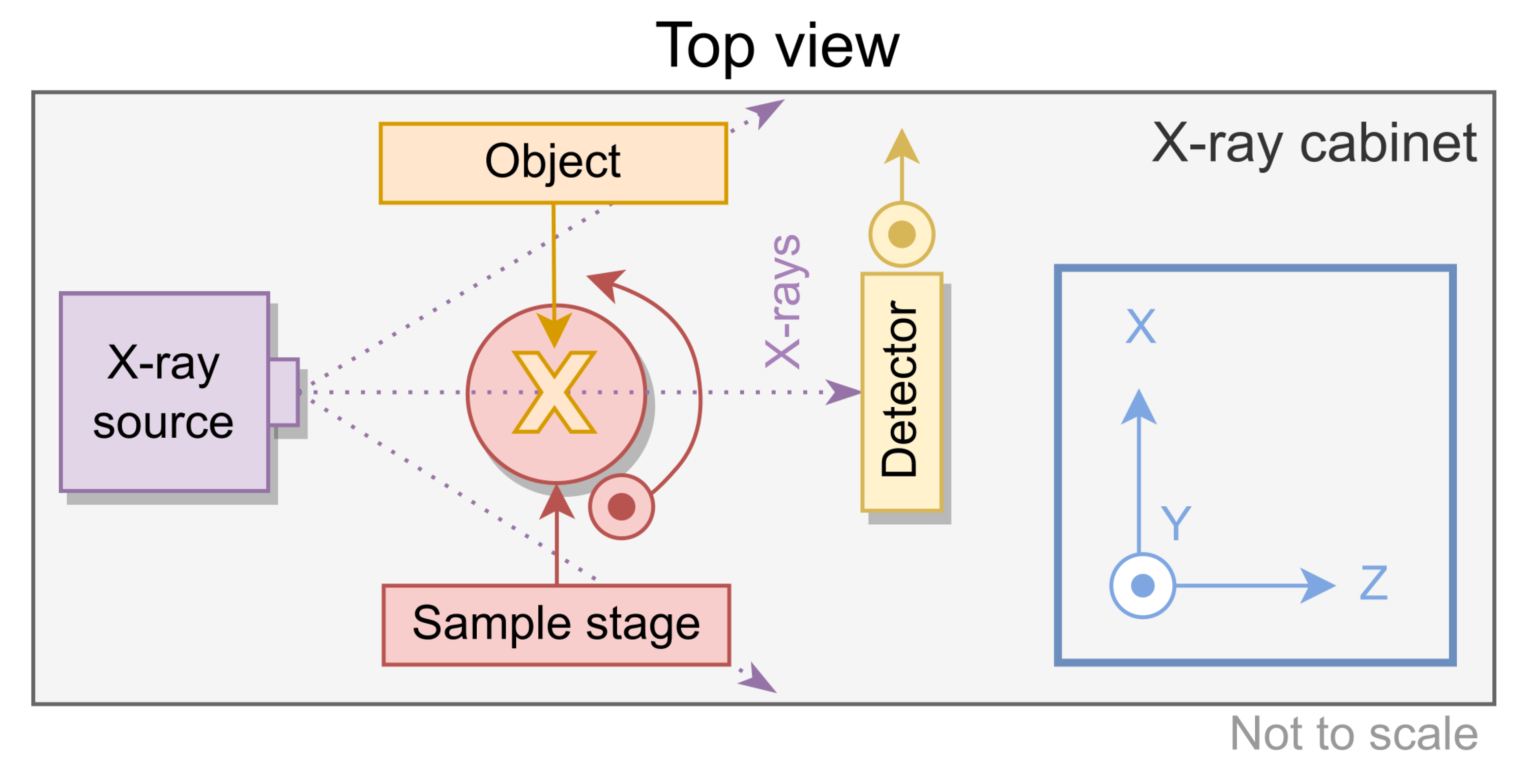
Figure 2.
A visual overview of the DAC shifting procedure. The inputs are energy dependent flat field data and energy dependent image data. The output is a set of corrected images. The red points are the flat field data for a single pixel and threshold, the dashed line between them is the fitted B-spline using a second order polynomial. The target is the median counts as a function of energy for the whole detector per threshold. The DAC-shifts are the per pixel differences in threshold between the flat field images and the target. Using these DAC-shifts, we find the corresponding point in the spline fit of the input data. This point is the corrected value in counts. The process is repeated for all pixels and thresholds and thus, the images are corrected.
Figure 2.
A visual overview of the DAC shifting procedure. The inputs are energy dependent flat field data and energy dependent image data. The output is a set of corrected images. The red points are the flat field data for a single pixel and threshold, the dashed line between them is the fitted B-spline using a second order polynomial. The target is the median counts as a function of energy for the whole detector per threshold. The DAC-shifts are the per pixel differences in threshold between the flat field images and the target. Using these DAC-shifts, we find the corresponding point in the spline fit of the input data. This point is the corrected value in counts. The process is repeated for all pixels and thresholds and thus, the images are corrected.
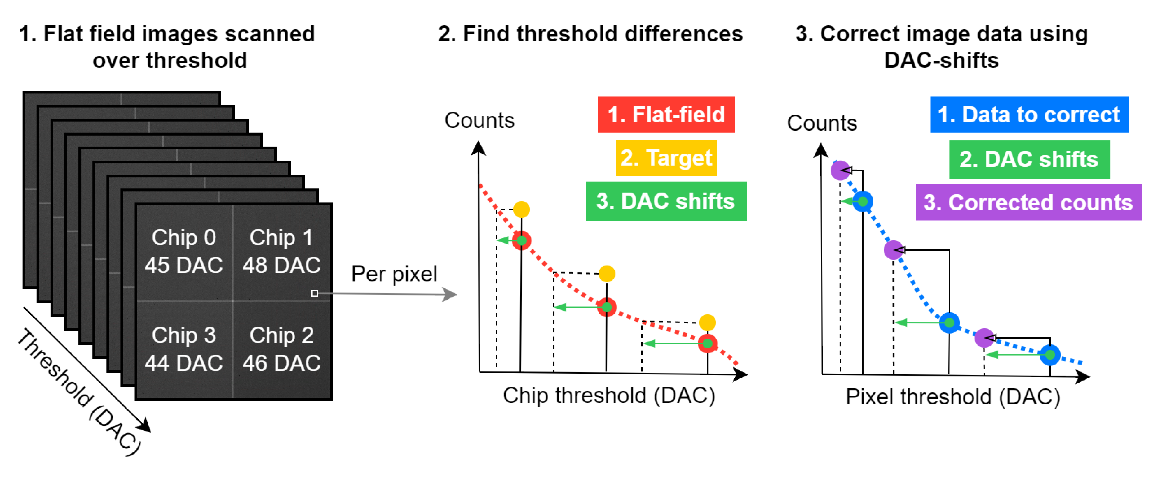
Figure 3.
Labelled diagram of a reconstructed slice of our custom microCT phantom. Each material has one unique colour; the excluded regions are the black margins. The black-white diagonal lines show the non-valid reconstruction region.
Figure 3.
Labelled diagram of a reconstructed slice of our custom microCT phantom. Each material has one unique colour; the excluded regions are the black margins. The black-white diagonal lines show the non-valid reconstruction region.
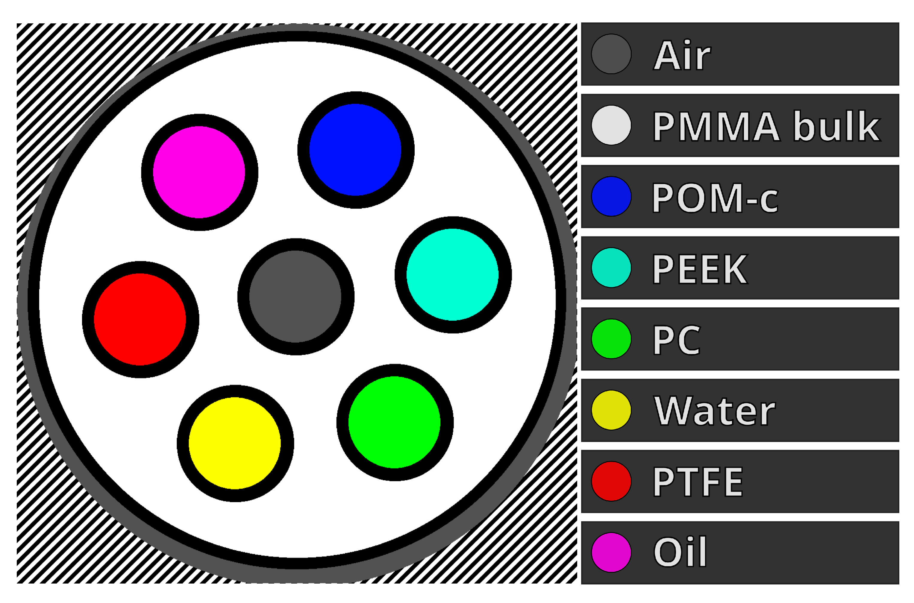
Figure 4.
An example reconstruction showing slices in each plane, XY, XZ and YZ. The grey scale is set to the full data range. The horizontal yellow line in the XZ plane show the slice used in subsequent plots.
Figure 4.
An example reconstruction showing slices in each plane, XY, XZ and YZ. The grey scale is set to the full data range. The horizontal yellow line in the XZ plane show the slice used in subsequent plots.
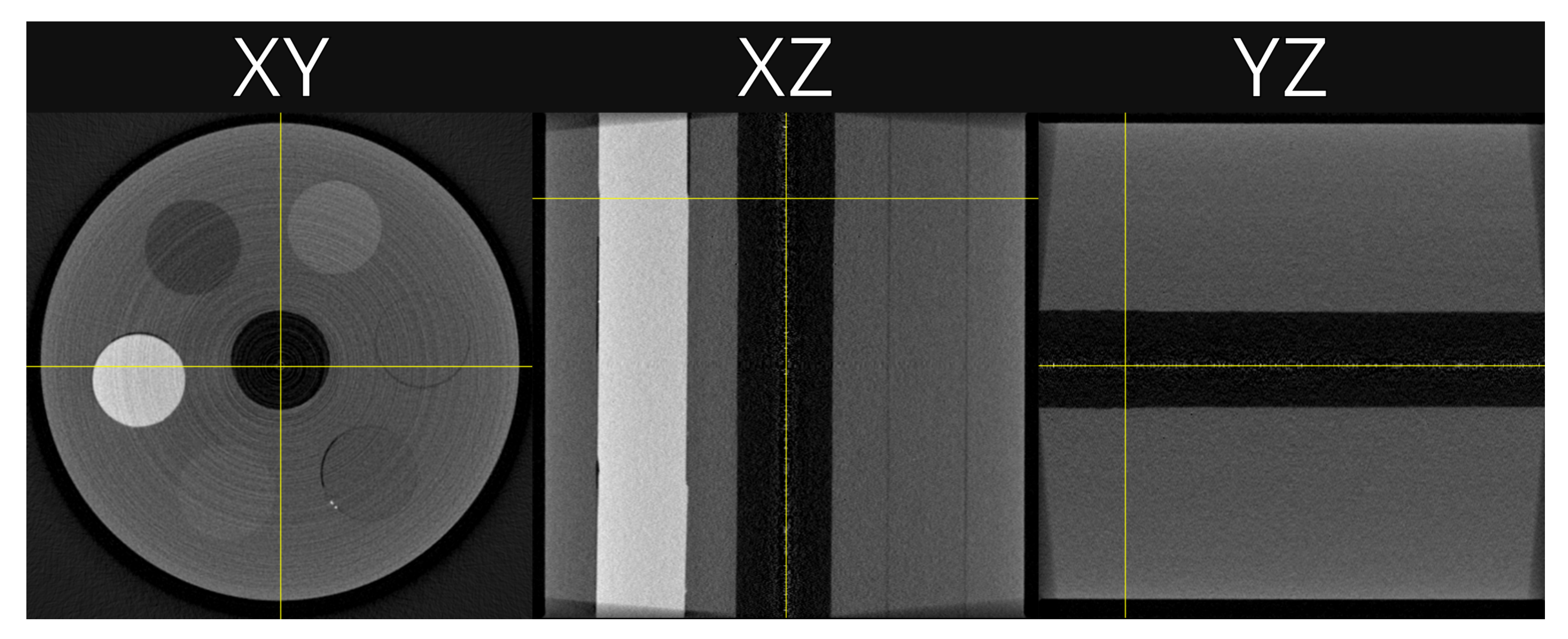
Figure 5.
DAC-shifted FISTA reconstructed CT slice of the iodine phantom at 33.0 keV with the manually segmented region marked in circles. The concentrations are ordered anti-clockwise starting from 135.0 mg/ml.
Figure 5.
DAC-shifted FISTA reconstructed CT slice of the iodine phantom at 33.0 keV with the manually segmented region marked in circles. The concentrations are ordered anti-clockwise starting from 135.0 mg/ml.
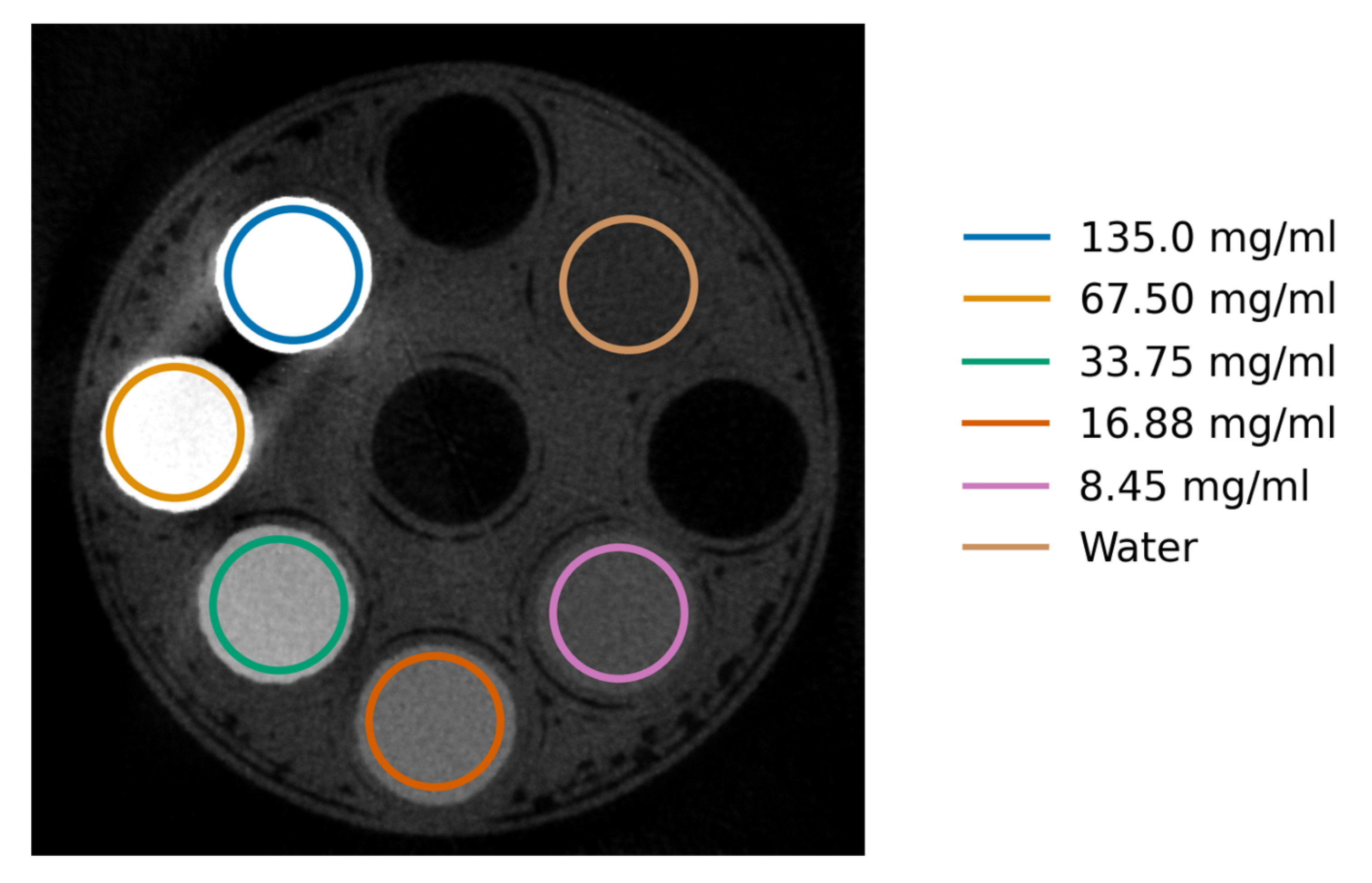
Figure 6.
Example reconstructions for two thresholds out-of-the-box (OOTB) and with a beam hardening correction (‘STC-D’). Top row: reconstructed slice at 5.0 (left) and 20.0 (right) keV for the most basic, out-of-the-box experience using the ASI detector (‘ASI-1’ data). The detector was not moved, no DAC-shifting, or any form of STC was used and FDK was used for reconstruction. Bottom row: the exact same reconstructions, but after using the STC-D beam hardening correction. In the middle of the image the profile of the yellow dotted lines is shown for the OOTB reconstructions in white, and the STC-D reconstructions in green.
Figure 6.
Example reconstructions for two thresholds out-of-the-box (OOTB) and with a beam hardening correction (‘STC-D’). Top row: reconstructed slice at 5.0 (left) and 20.0 (right) keV for the most basic, out-of-the-box experience using the ASI detector (‘ASI-1’ data). The detector was not moved, no DAC-shifting, or any form of STC was used and FDK was used for reconstruction. Bottom row: the exact same reconstructions, but after using the STC-D beam hardening correction. In the middle of the image the profile of the yellow dotted lines is shown for the OOTB reconstructions in white, and the STC-D reconstructions in green.
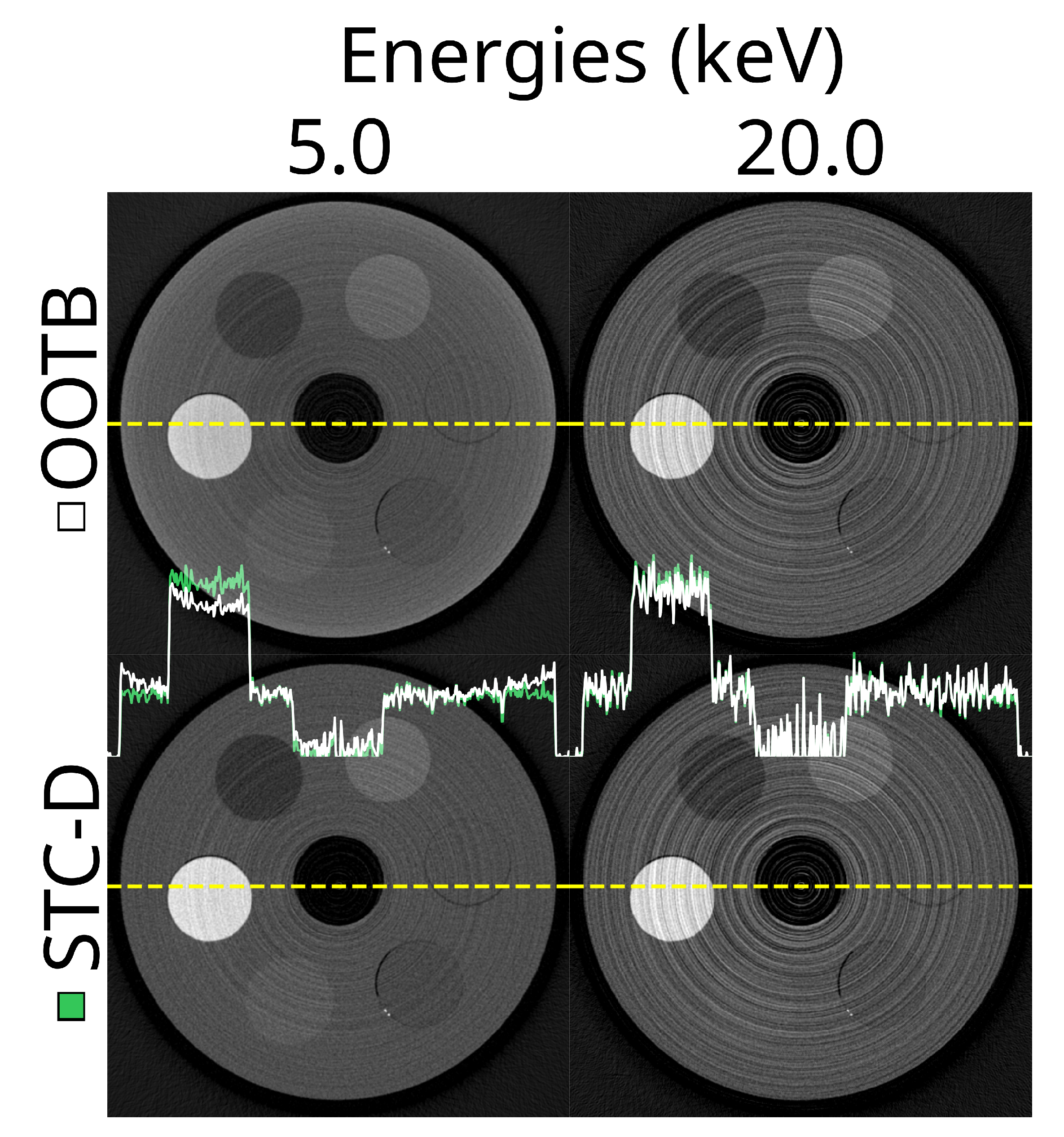
Figure 7.
The median reconstructed CT number per material over energy using the ASI detector for the most basic out-of-the-box configuration. The colour bands represent the 95th percentile range within each material. The scan (‘ASI-1’ dataset) was made using FDK reconstruction, no detector motion, no signal-to-thickness calibration, and no DAC-shifting. The corresponding median of all percentile sizes for this data is 234 HU.
Figure 7.
The median reconstructed CT number per material over energy using the ASI detector for the most basic out-of-the-box configuration. The colour bands represent the 95th percentile range within each material. The scan (‘ASI-1’ dataset) was made using FDK reconstruction, no detector motion, no signal-to-thickness calibration, and no DAC-shifting. The corresponding median of all percentile sizes for this data is 234 HU.
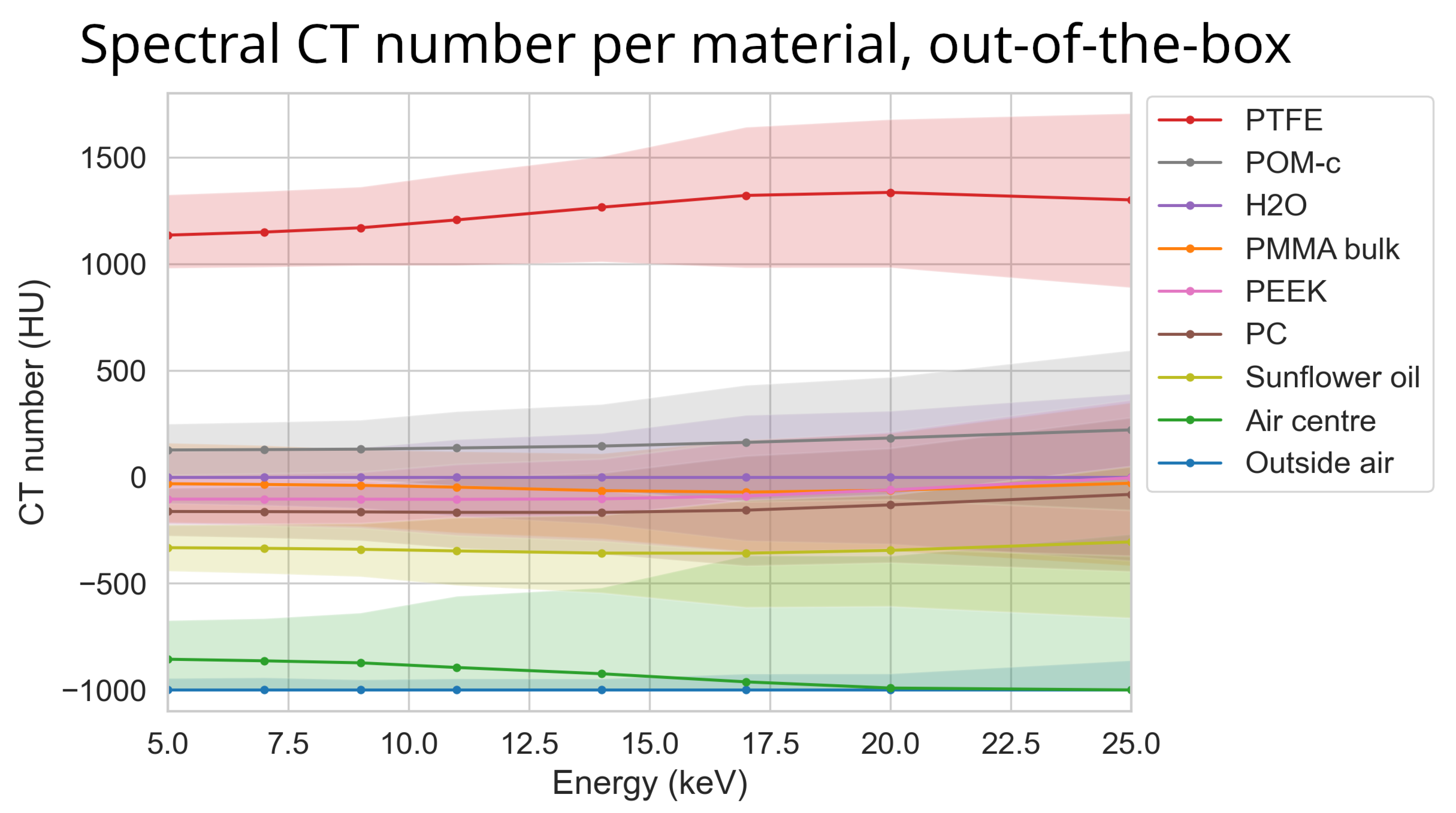
Figure 8.
The same reconstructed slice for two energy thresholds (5.0 and 20.0 keV) and without and with detector motion. The reconstructions are from the ASI-1 data, with STC-D beam hardening correction, DAC-shifting, and FDK reconstruction.
Figure 8.
The same reconstructed slice for two energy thresholds (5.0 and 20.0 keV) and without and with detector motion. The reconstructions are from the ASI-1 data, with STC-D beam hardening correction, DAC-shifting, and FDK reconstruction.
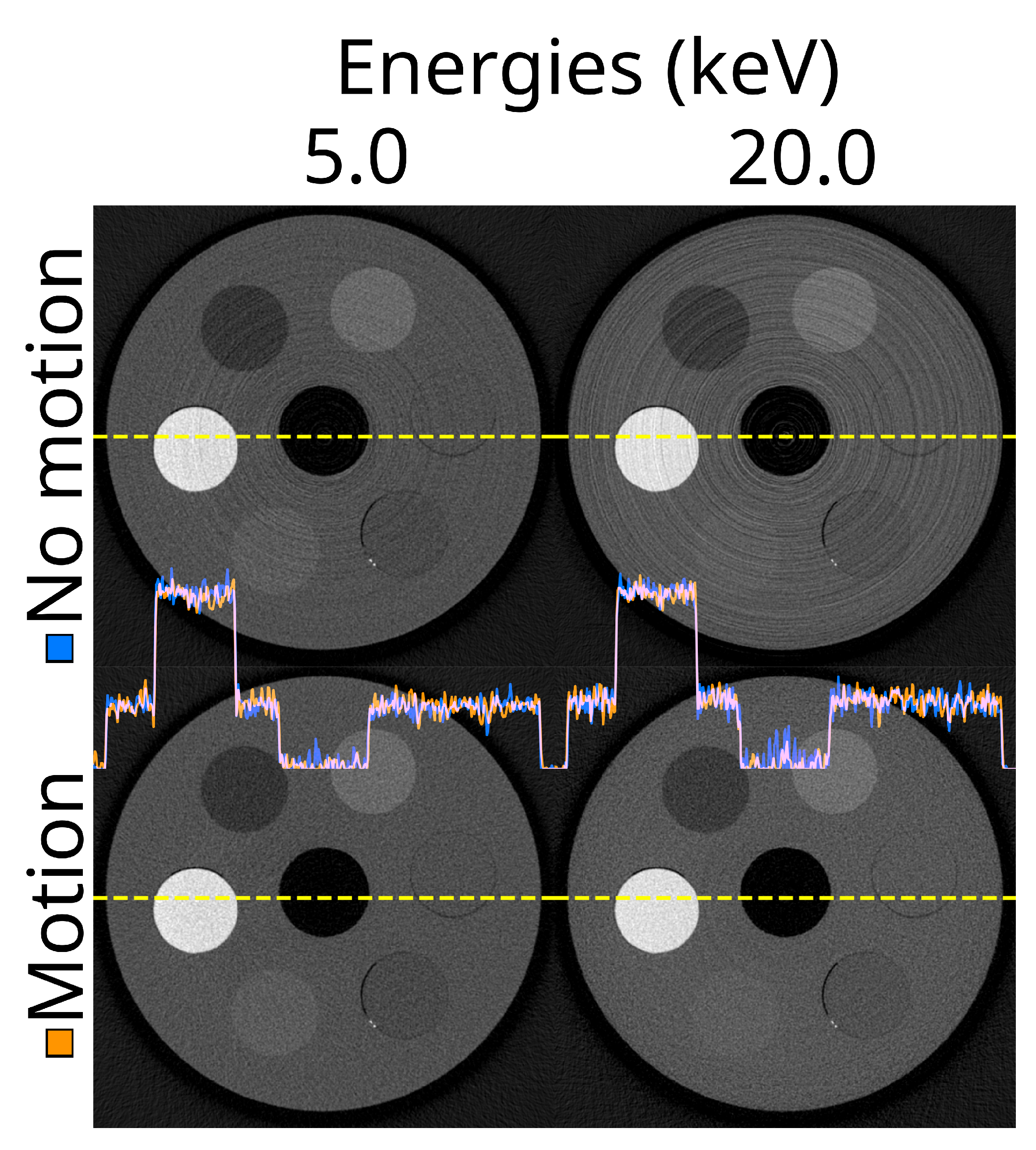
Figure 9.
Paired mean of median percentile sizes between without and with detector motion, for all datasets and all combinations of reconstruction type, DAC-shifting, STC-P and STC-D. Note that these comparisons are actually comparisons between different acquisitions, as detector motion was an acquisition parameter, not a post-processing method.
Figure 9.
Paired mean of median percentile sizes between without and with detector motion, for all datasets and all combinations of reconstruction type, DAC-shifting, STC-P and STC-D. Note that these comparisons are actually comparisons between different acquisitions, as detector motion was an acquisition parameter, not a post-processing method.
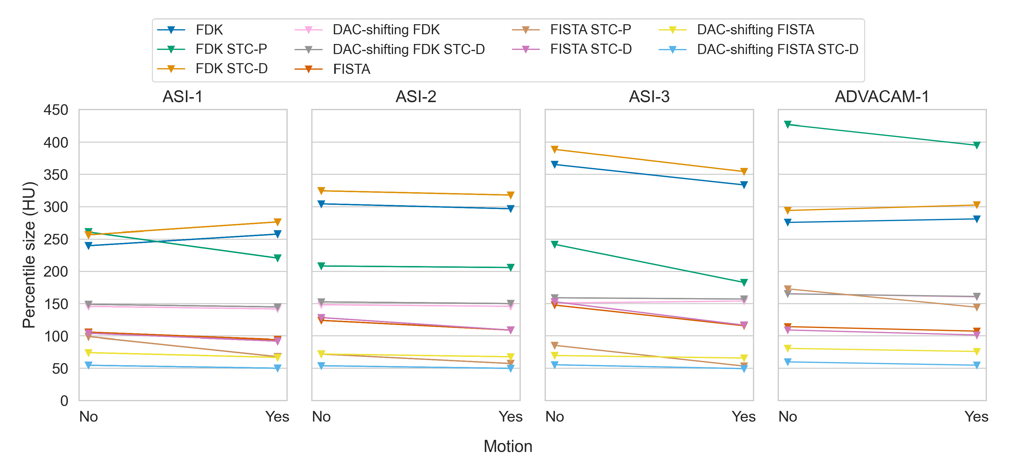
Figure 10.
Paired mean of median percentile sizes between without and with STC-P, for all datasets and all combinations of reconstruction type and detector motion.
Figure 10.
Paired mean of median percentile sizes between without and with STC-P, for all datasets and all combinations of reconstruction type and detector motion.
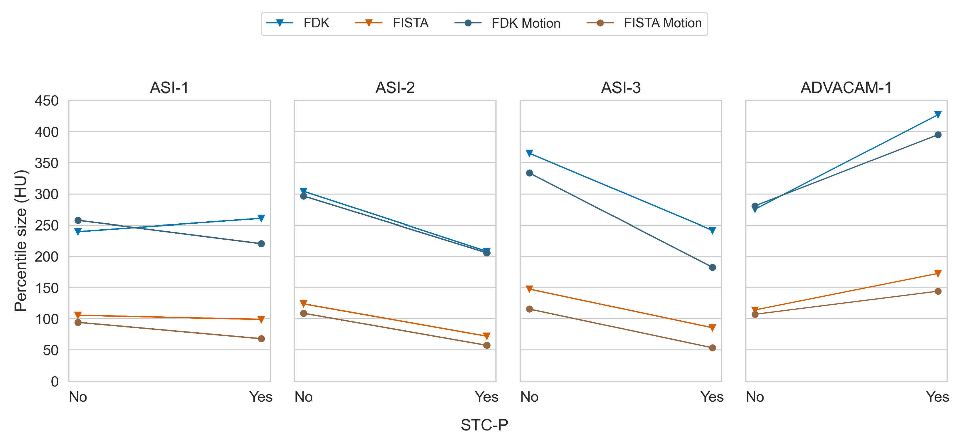
Figure 11.
The same slice at 20.0 keV when using the signal to thickness calibration with detector wide data (STC-D) compared to per pixel data (STC-P). The top row is based on the ‘ASI-1’ data, and the bottom row based on ‘ASI-3’. The viewing window is set to -1000 — 1800 HU for all subplots.
Figure 11.
The same slice at 20.0 keV when using the signal to thickness calibration with detector wide data (STC-D) compared to per pixel data (STC-P). The top row is based on the ‘ASI-1’ data, and the bottom row based on ‘ASI-3’. The viewing window is set to -1000 — 1800 HU for all subplots.
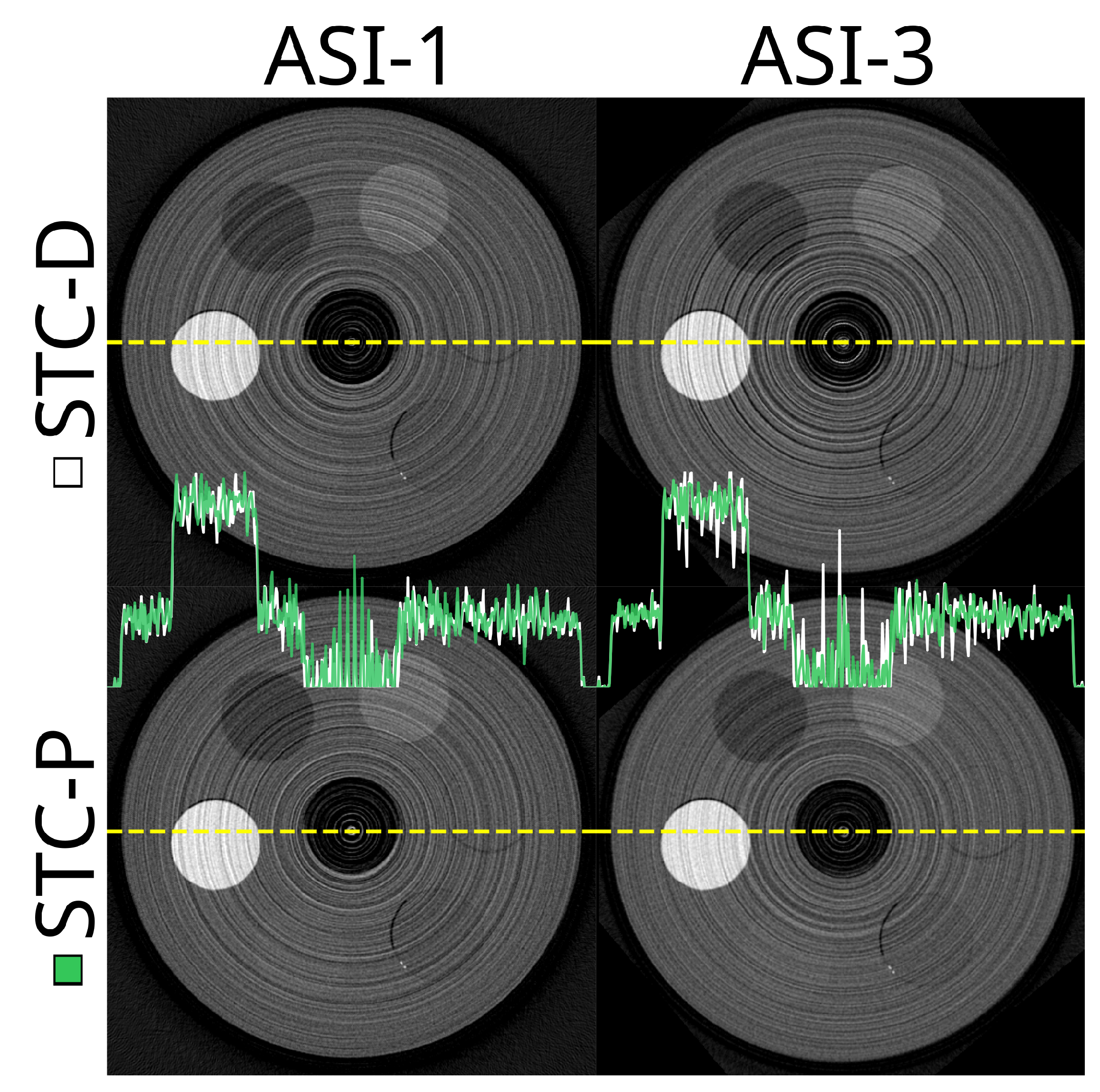
Figure 12.
The corrected DAC distributions (LUT) and their standard deviations as a function of dataset at 14.0 keV. a) The corrected DAC distribution image of the first dataset (#1), the first LUT. b) The corresponding histogram of that image. c) The standard deviation () of all six ASI datasets at 14.0 keV. The window size is set from 0 — 99 % (0 — 5.80 DAC units), green pixels are above the upper window level. d) The corresponding histogram of c, with the same 99 % window size indicated with vertical black lines. The dataset numbers are detailed in Table 2.
Figure 12.
The corrected DAC distributions (LUT) and their standard deviations as a function of dataset at 14.0 keV. a) The corrected DAC distribution image of the first dataset (#1), the first LUT. b) The corresponding histogram of that image. c) The standard deviation () of all six ASI datasets at 14.0 keV. The window size is set from 0 — 99 % (0 — 5.80 DAC units), green pixels are above the upper window level. d) The corresponding histogram of c, with the same 99 % window size indicated with vertical black lines. The dataset numbers are detailed in Table 2.
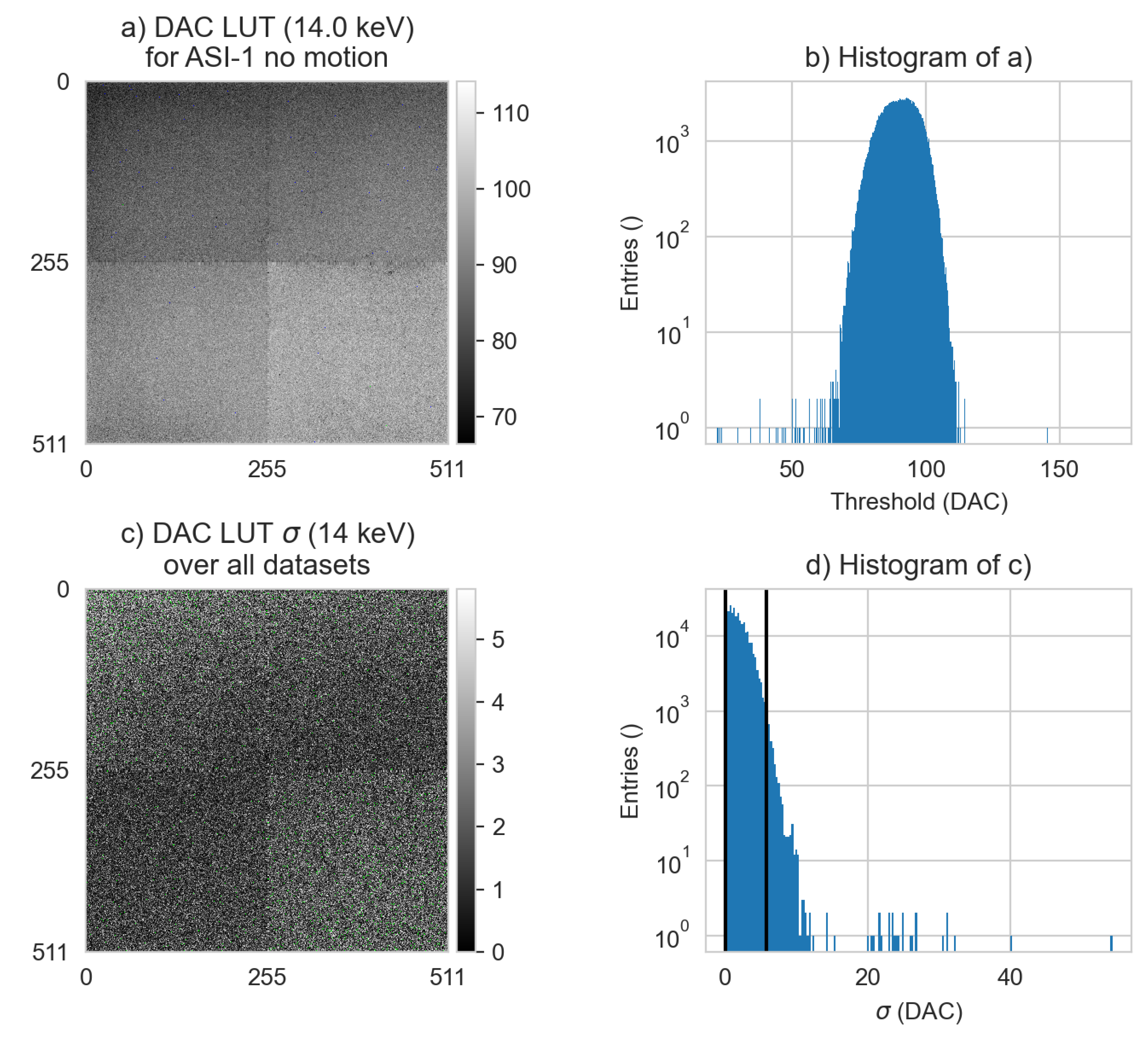
Figure 13.
The sinograms and projections of OOTB (‘out-of-the-box’), DAC-shifted, STC-P data and the differences between two of the pairs. The threshold is set to 9.0 or 25.0 keV respectively from left to right. The projections are an arbitrarily selected slice, 88 of 510, from the corresponding sinograms. The viewing windows are all set to 0.1 — 99.9 % of the range per image. In the last row the difference between DAC-shifting (in b), and OOTB (in a) is shown to illustrate the DAC-shifting correction. The ‘ASI-3’ no motion dataset was used.
Figure 13.
The sinograms and projections of OOTB (‘out-of-the-box’), DAC-shifted, STC-P data and the differences between two of the pairs. The threshold is set to 9.0 or 25.0 keV respectively from left to right. The projections are an arbitrarily selected slice, 88 of 510, from the corresponding sinograms. The viewing windows are all set to 0.1 — 99.9 % of the range per image. In the last row the difference between DAC-shifting (in b), and OOTB (in a) is shown to illustrate the DAC-shifting correction. The ‘ASI-3’ no motion dataset was used.
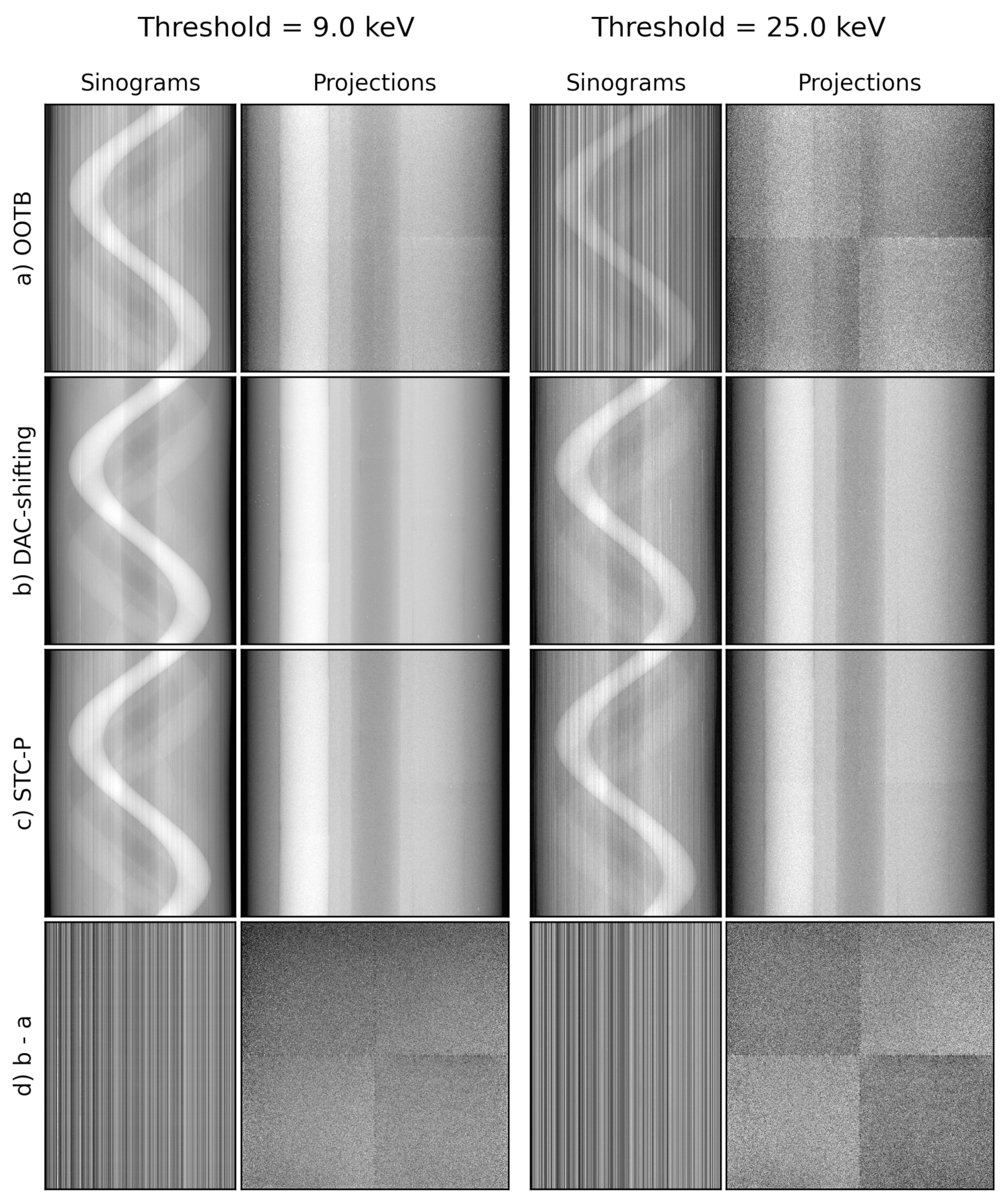
Figure 14.
Example reconstructions for different thresholds with and without DAC-shifting. Top row: FDK reconstructed slice at 5.0 (left) and 20.0 (right) keV using a static detector, STC-D, and no DAC-shifting. The lower row is showing the exact same reconstructions, but with DAC-shifting enabled. In the middle of the image, the profile of the yellow dotted lines is green for the top row, and the lower row is blue.
Figure 14.
Example reconstructions for different thresholds with and without DAC-shifting. Top row: FDK reconstructed slice at 5.0 (left) and 20.0 (right) keV using a static detector, STC-D, and no DAC-shifting. The lower row is showing the exact same reconstructions, but with DAC-shifting enabled. In the middle of the image, the profile of the yellow dotted lines is green for the top row, and the lower row is blue.
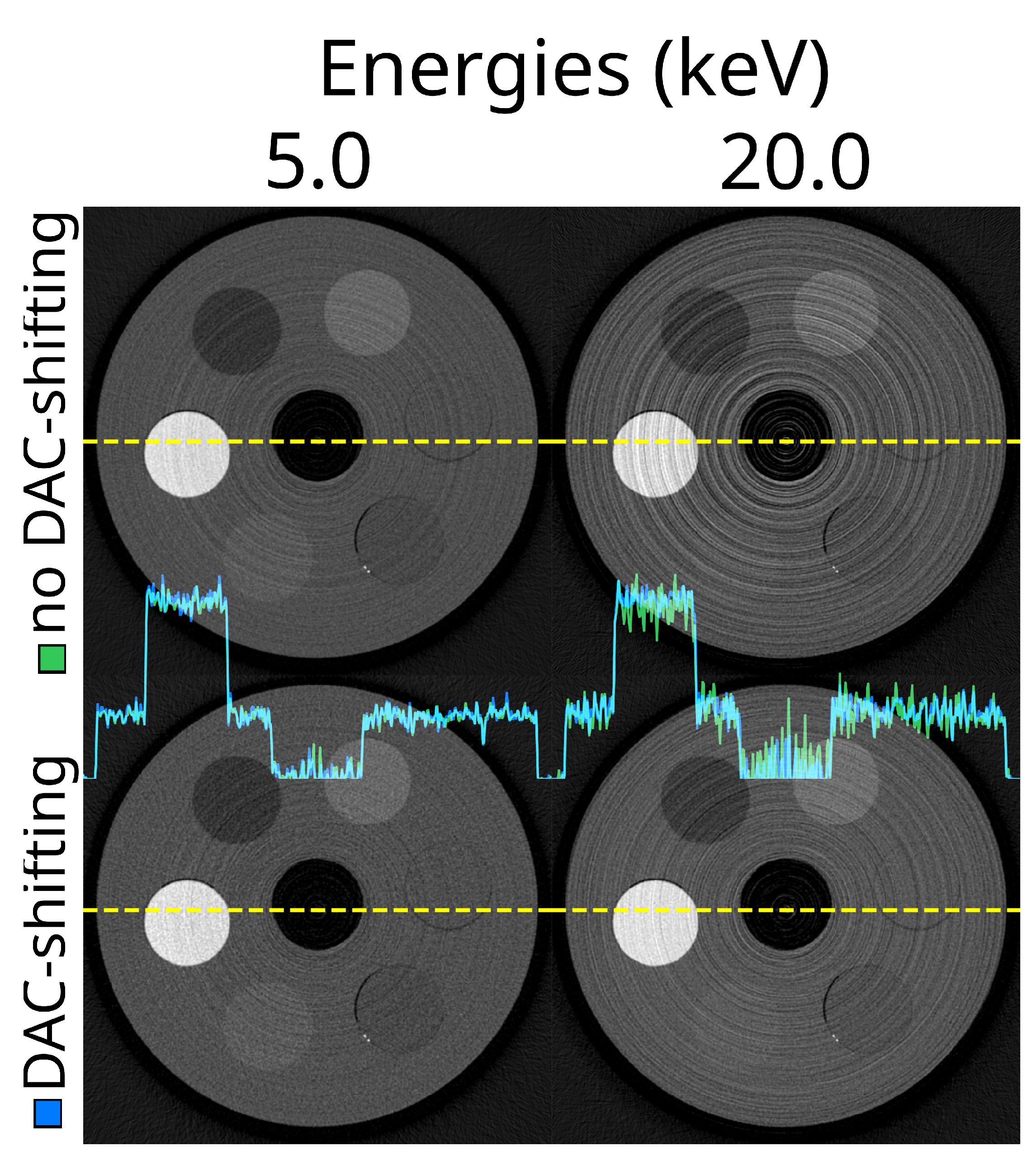
Figure 15.
Paired mean of median percentile sizes between without and with DAC-shifting, for all datasets and all combinations of reconstruction type, detector motion, and STC-D.
Figure 15.
Paired mean of median percentile sizes between without and with DAC-shifting, for all datasets and all combinations of reconstruction type, detector motion, and STC-D.
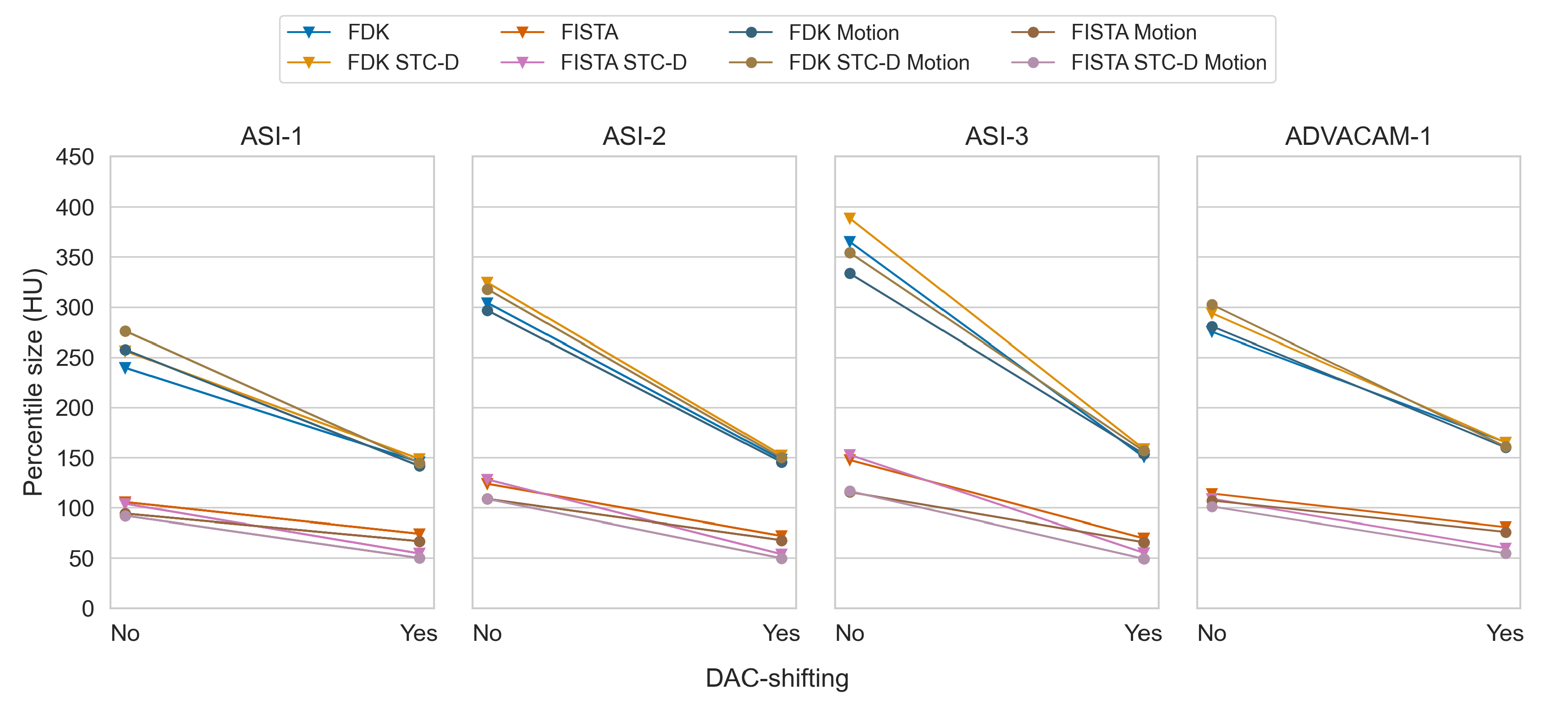
Figure 16.
The same reconstructed slice for two energy thresholds (5.0 and 20.0 keV) using the FDK (non-iterative) and FISTA (iterative) reconstruction methods. This is using the ASI detector (ASI-1), the STC-D beam hardening correction, detector motion and DAC-shifting.
Figure 16.
The same reconstructed slice for two energy thresholds (5.0 and 20.0 keV) using the FDK (non-iterative) and FISTA (iterative) reconstruction methods. This is using the ASI detector (ASI-1), the STC-D beam hardening correction, detector motion and DAC-shifting.
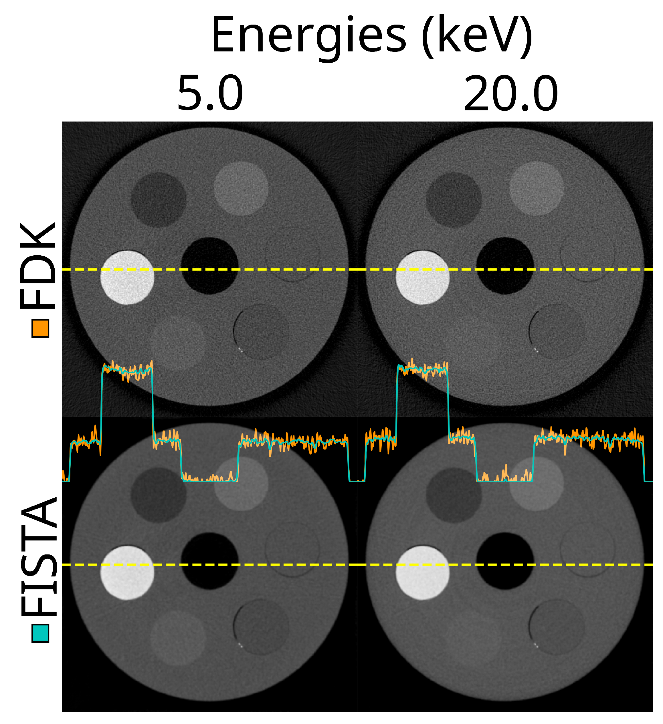
Figure 17.
The same reconstructed slice for two energy thresholds (5.0 and 20.0 keV) using the out-of –the-box approach with FISTA, no DAC-shifting, no STC, no detector motion (top row), and the best combination of all options (lower row). This is using the ASI detector (ASI-1). For the ‘best’ combination, STC-D, detector motion, DAC-shifting and the FISTA reconstruction method are used.
Figure 17.
The same reconstructed slice for two energy thresholds (5.0 and 20.0 keV) using the out-of –the-box approach with FISTA, no DAC-shifting, no STC, no detector motion (top row), and the best combination of all options (lower row). This is using the ASI detector (ASI-1). For the ‘best’ combination, STC-D, detector motion, DAC-shifting and the FISTA reconstruction method are used.
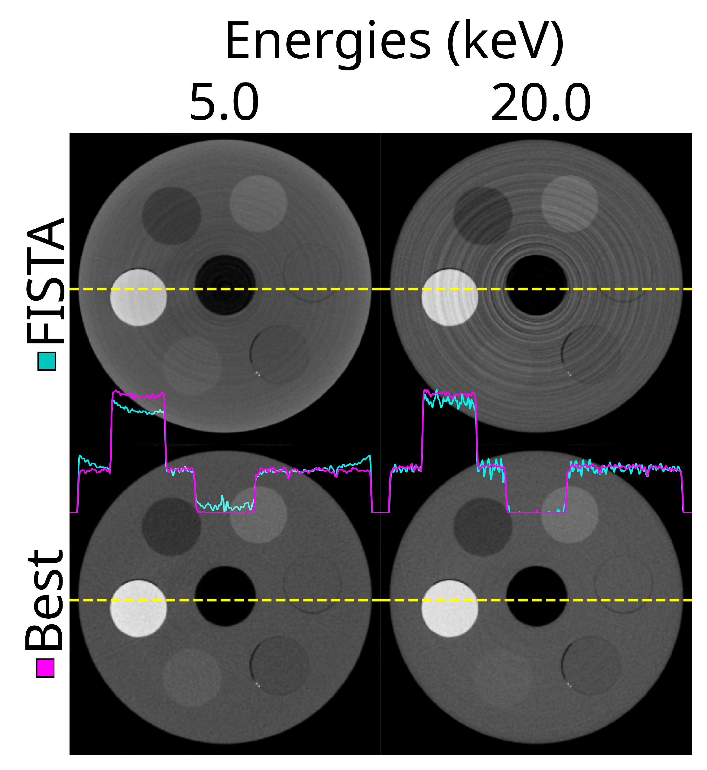
Figure 18.
The reconstructed CT number per material over energy using the ASI detector for the best parameter combination. Here STC-D, detector motion, DAC-shifting and the FISTA reconstruction methods are used on the ‘ASI-1’ dataset. The corresponding mean percentile size for this data was 49 HU.
Figure 18.
The reconstructed CT number per material over energy using the ASI detector for the best parameter combination. Here STC-D, detector motion, DAC-shifting and the FISTA reconstruction methods are used on the ‘ASI-1’ dataset. The corresponding mean percentile size for this data was 49 HU.
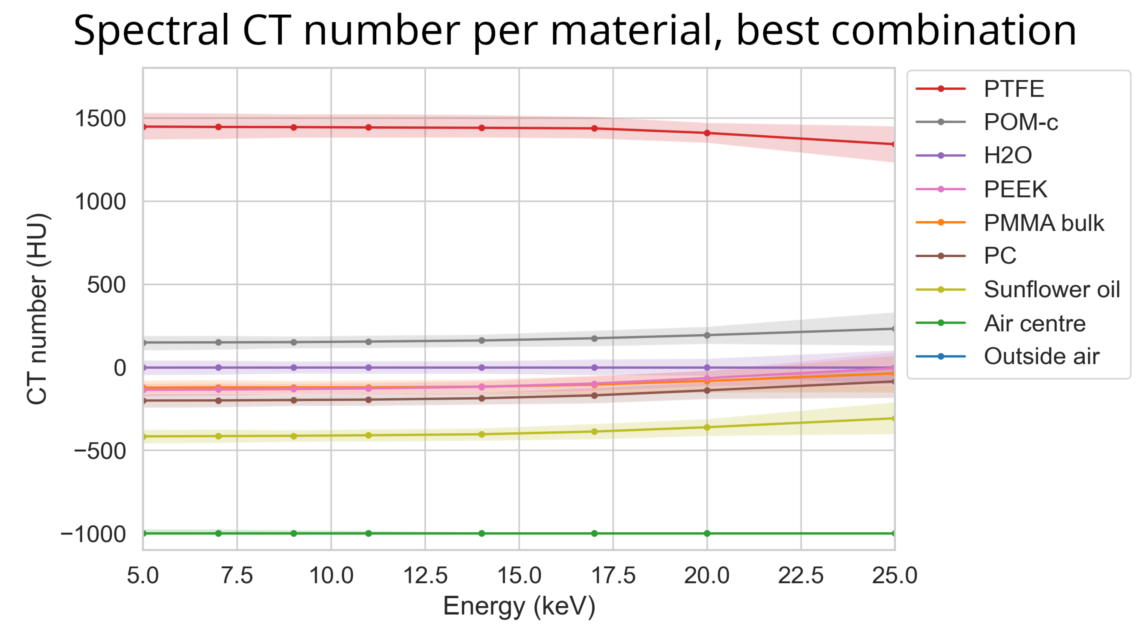
Figure 19.
The top row shows a series of attenuation images at various thresholds (15.5, 26.0, 30.5, 33.0, and 40.5 keV) acquired without DAC-shifting. The second row displays images at the same energy level with DAC-shifting. On the bottom row, the plot shows the mean attenuation as function of energy (at 0.5 keV interval) and the 95 % data distribution of all chips combined for without and with DAC-shifting. The vertical dashed line indicates the K-edge of iodine (33.2 keV) and the green dotted lines indicate the corresponding thresholds presented in the top rows.
Figure 19.
The top row shows a series of attenuation images at various thresholds (15.5, 26.0, 30.5, 33.0, and 40.5 keV) acquired without DAC-shifting. The second row displays images at the same energy level with DAC-shifting. On the bottom row, the plot shows the mean attenuation as function of energy (at 0.5 keV interval) and the 95 % data distribution of all chips combined for without and with DAC-shifting. The vertical dashed line indicates the K-edge of iodine (33.2 keV) and the green dotted lines indicate the corresponding thresholds presented in the top rows.
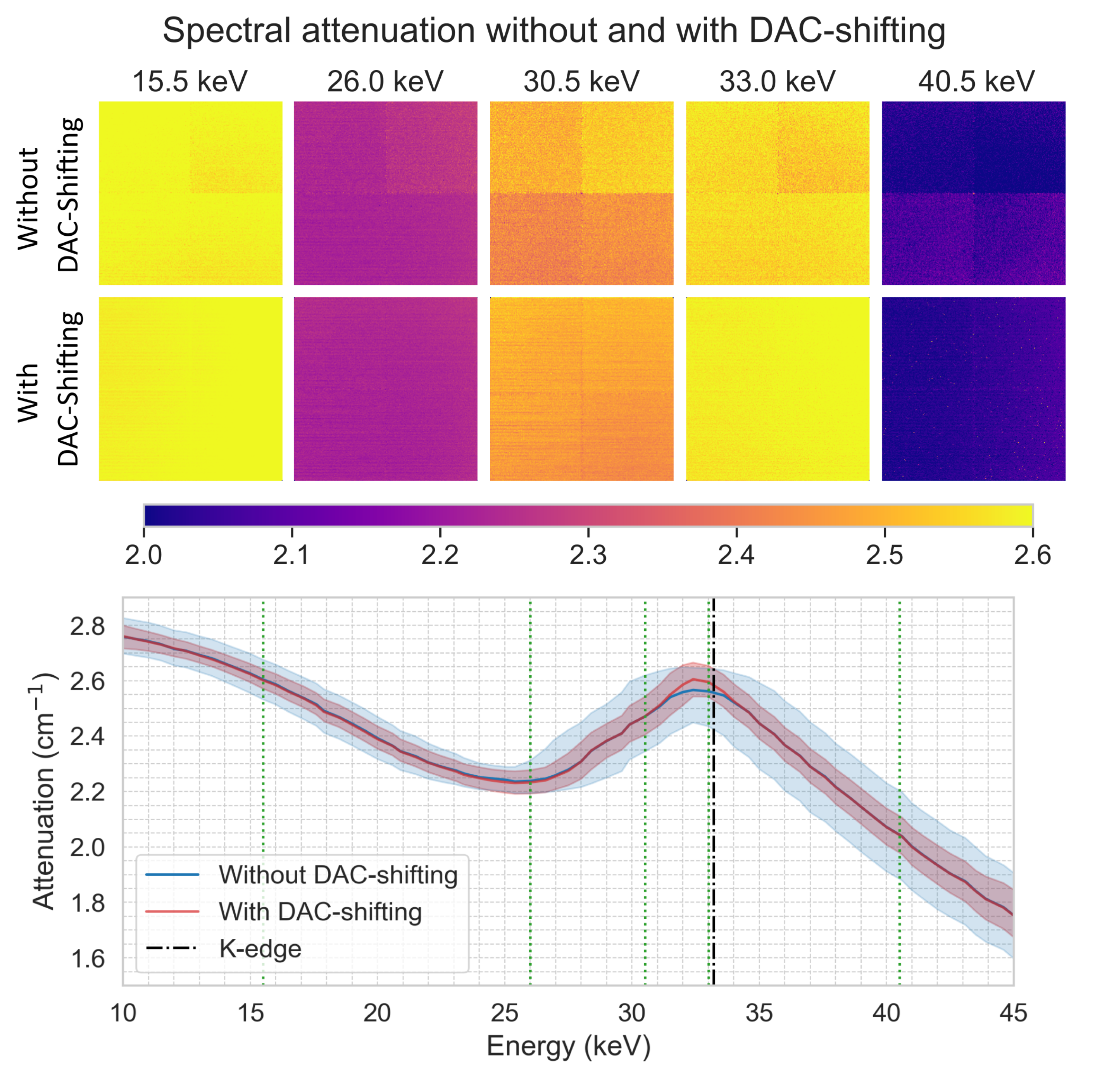
Figure 20.
Spectral profiles and concentration calibration for iodine solutions. Top row displays the CT numbers in Hounsfield Units (HU) across a range of energies for iodine concentrations at 135.0, 67.50, 33.75, 16.88, and 8.45 mg/ml, as well as water, without (top left) DAC-shifting using FISTA reconstruction and with (top right) DAC-shifting using FISTA reconstruction. The vertical dashed lines indicate the K-edge of Iodine (33.2 keV). The bottom row illustrates the linear relationship between varying iodine concentration at 33.0 keV for FISTA without DAC-shifting (bottom left) and FISTA with DAC-shifting (bottom right) and their corresponding CT numbers along with the 95 % distribution of the data as vertical error bars.
Figure 20.
Spectral profiles and concentration calibration for iodine solutions. Top row displays the CT numbers in Hounsfield Units (HU) across a range of energies for iodine concentrations at 135.0, 67.50, 33.75, 16.88, and 8.45 mg/ml, as well as water, without (top left) DAC-shifting using FISTA reconstruction and with (top right) DAC-shifting using FISTA reconstruction. The vertical dashed lines indicate the K-edge of Iodine (33.2 keV). The bottom row illustrates the linear relationship between varying iodine concentration at 33.0 keV for FISTA without DAC-shifting (bottom left) and FISTA with DAC-shifting (bottom right) and their corresponding CT numbers along with the 95 % distribution of the data as vertical error bars.
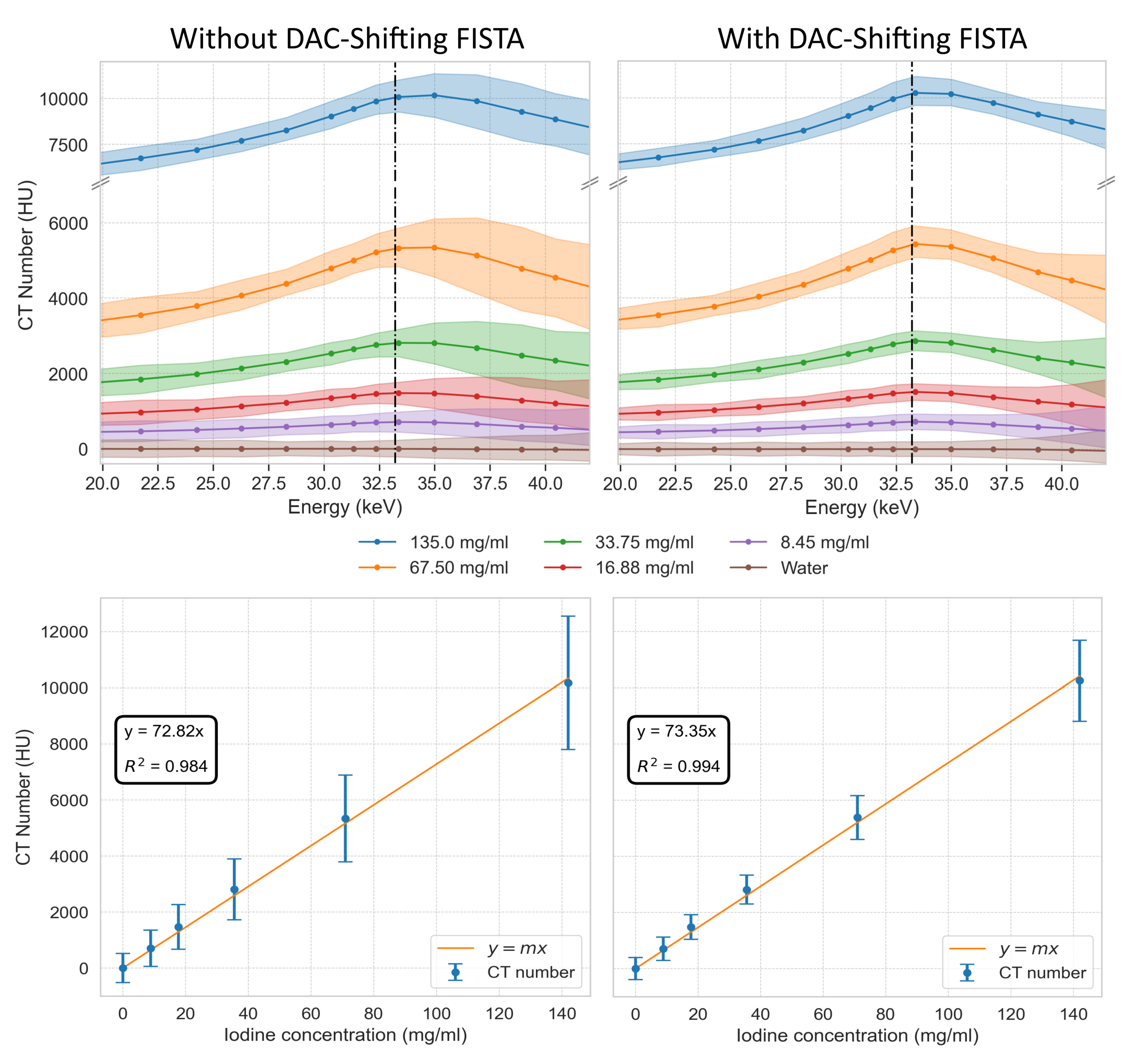

Table 1.
An overview of the thresholds and exposure times used in the acquisitions.
| Acquisition # | Threshold 0 (keV) | Threshold 1 (keV) | Exposure time (s) |
|---|---|---|---|
| 1 | 5.0 | 7.0 | 2.08 |
| 2 | 9.0 | 11.0 | 2.88 |
| 3 | 14.0 | 17.0 | 4.48 |
| 4 | 20.0 | 25.0 | 9.60 |
| 5 | 25.0 | 30.0 | 9.60 |
Table 2.
Overview of the measurements performed. On 20-12-2023 the measurements were done for the STC calibration of both detectors.
Table 2.
Overview of the measurements performed. On 20-12-2023 the measurements were done for the STC calibration of both detectors.
| Measurement # | Date | Manufacturer | Motion | Days difference to STC calibration | Dataset name |
|---|---|---|---|---|---|
| 1 | 29-11-2023 | ASI | No | -22 | ASI-1 |
| 2 | Yes | ||||
| 3 | 30-11-2023 | ADVACAM | No | -21 | ADVACAM-1 |
| 4 | Yes | ||||
| 5 | 19-12-2023 | ASI | No | -1 | ASI-2 |
| 6 | Yes | ||||
| 7 | 23-12-2023 | ASI | Yes | +3 | ASI-3 |
| 8 | 24-12-2023 | No | +4 |
Table 3.
Overview of the acquisition numbers, thresholds and exposure times used in the 3D spectral CT acquisition of different iodine concentrations.
Table 3.
Overview of the acquisition numbers, thresholds and exposure times used in the 3D spectral CT acquisition of different iodine concentrations.
| Acquisition # | Threshold 0 (keV) | Threshold 1 (keV) | Exposure time (s) |
|---|---|---|---|
| 1 | 19.5 | 21.5 | 1.10 |
| 2 | 24.0 | 26.0 | 1.66 |
| 3 | 28.0 | 30.0 | 3.04 |
| 4 | 31.0 | 32.0 | 4.00 |
| 5 | 33.0 | 35.0 | 5.10 |
| 6 | 35.0 | 37.0 | 6.04 |
| 7 | 37.0 | 39.0 | 7.44 |
| 8 | 40.5 | 42.5 | 10.0 |
| 9 | 42.5 | 44.5 | 10.0 |
Table 4.
Overview of the effectiveness scores comparing the different options for improving image quality on the different datasets. The ‘combined’ row is the result of the same analysis as individual datasets but using all datasets listed. The numbers listed are the effectiveness scores (mean and IQR) as a percentage change, followed by the p-value (significant findings are shown in bold).
Table 4.
Overview of the effectiveness scores comparing the different options for improving image quality on the different datasets. The ‘combined’ row is the result of the same analysis as individual datasets but using all datasets listed. The numbers listed are the effectiveness scores (mean and IQR) as a percentage change, followed by the p-value (significant findings are shown in bold).
| Datasets | STC-D | Detector motion | STC-P | DAC-shifting | Reconstruction type |
|---|---|---|---|---|---|
| ASI-1 | -4.6 (-7.9 : +3.4) p = 0.97 |
-7.8 (-11.3 : -2.7) p = 0.22 |
-10.0 (-17.8 : -2.5) p = 0.41 |
-40.7 (-46.1 : -36.9) p = 0.001 |
-60.7 (-64.9 : -56.8) p < 0.001 |
| ASI-2 | -3.6 (-6.3 : +4.3) p = 0.67 |
-7.0 (-11.0 : -1.8) p < 0.001 |
-37.8 (-43.2 : -31.3) p < 0.001 |
-50.0 (-53.3 : -48.6) p < 0.001 |
-62.3 (-65.7 : -59.6) p < 0.001 |
| ASI-3 | -2.7 (-4.5 : +5.6) p = 0.48 |
-14.1 (-23.3 : -6.4) p < 0.001 |
-43.7 (-47.4 : -40.0) p < 0.001 |
-55.6 (-58.8 : -53.6) p < 0.001 |
-63.3 (-66.7 : -59.9) p < 0.001 |
| ADVACAM-1 | -6.2 (-10.7 : +2.1) p < 0.78 |
-5.3 (-7.4 : -2.6) p = 0.08 |
+45.5 (+39.2 : +52.3) p = 0.04 |
-40.3 (-45.2 : -37.3) p = 0.002 |
-60.6 (-63.7 : -58.8) p < 0.001 |
| Combined | -4.2 (-7.4 : +3.6) p = 0.83 |
-8.7 (-13.0 : -1.5) p < 0.001 |
-13.7 (-16.6 : -10.4) p < 0.001 |
-47.4 (-51.1 : -46.3) p < 0.001 |
-61.6 (-66.0 : -59.1) p < 0.001 |
Disclaimer/Publisher’s Note: The statements, opinions and data contained in all publications are solely those of the individual author(s) and contributor(s) and not of MDPI and/or the editor(s). MDPI and/or the editor(s) disclaim responsibility for any injury to people or property resulting from any ideas, methods, instructions or products referred to in the content. |
© 2024 by the authors. Licensee MDPI, Basel, Switzerland. This article is an open access article distributed under the terms and conditions of the Creative Commons Attribution (CC BY) license (http://creativecommons.org/licenses/by/4.0/).
Copyright: This open access article is published under a Creative Commons CC BY 4.0 license, which permit the free download, distribution, and reuse, provided that the author and preprint are cited in any reuse.


