
Submitted:
30 May 2024
Posted:
31 May 2024
You are already at the latest version
Abstract
Environmental chemicals, including PFAS (per- and polyfluoroalkyl substances), pesticides, industrial chemicals, and consumer products, commonly exist as mixtures. These substances are frequently exposed or co-exposed in varying concentrations, leading to potentially hazardous health effects such as cancer in humans. Thus, understanding the dose-dependent toxicity of chemical mixtures is important for assessing health risks. In this context, comprehensive methods for assessing the toxicity and identifying the mechanisms of harmful chemical mixtures are currently lacking. Here, the dose-dependent toxicity assessments of chemical mixtures are performed in three methodologically distinct phases. In the first phase, we evaluated our machine learning method (AI-HNN) and pathophysiology method (CPTM) for predicting toxicity. In the second phase, we integrated AI-HNN and CPTM to establish a comprehensive new approach method (NAM) framework called AI-CPTM, targeted at refining prediction accuracy and providing a comprehensive understanding of toxicity mechanisms. The third phase involved experimental validations of the AI-CPTM predictions. Initially, we developed binary, multiclass classification, and regression models to predict binary, categorical toxicity, and toxic potencies, using nearly a thousand experimental mixtures. This empirical dataset was expanded with virtual mixtures compensating the lack of experimental data and broadening the scope of the dataset. For comparison, we also developed additional machine learning models based on RF, Bagging, AdaBoost, SVR, GB, KR, DT, KN, and Consensus methods. The models achieved overall accuracies of over 80% with AUC values exceeding 90%. The regression models achieved an R2 >0.88. In the second phase, we innovatively integrated HNN-derived toxicity predictions with Z-scores from CPTM, resulting method called AI-CPTM. In the final phase, we demonstrated the superior performance of AI-CPTM through rigorous literature and statistical performance validations. Additionally, the predictive capability of AI-CPTM, including for PFAS mixtures and their interaction effects, was demonstrated by experimental validations using dose-response zebrafish embryo toxicity assays. Overall, the AI-CPTM approach significantly improves upon the limitations of standalone models and has shown extensive enrichments in the identification of toxic chemicals and mixtures. Further experimental studies involving human cell models, patient-derived xenografts, and investigations into the toxicity of multiple mixtures are currently underway.
Keywords:
Environmental chemicals
; mixtures
; PFAS
; NAM method
; Toxicity
; zebrafish toxicity
Introduction
Humans are routinely coexposed to various chemicals present in the environment. These environmental chemicals mostly exist as mixtures of diverse individual chemicals. The toxicity of these mixtures is significantly influenced by the concentration levels of their individual components. While the toxicity profiles of single chemicals have been widely studied and reported, there is a substantial gap in comprehensive data regarding the toxicity of chemical mixtures. This lack of experimental toxicity data on chemical mixtures is due to several associated difficulties including high costs, time-consuming processes, and ethical issues related to the use of animals in toxicological testing [1]. The practical challenges of conducting experimental evaluations on chemical mixtures are further augmented by the existence of number of potential combinations and concentration ratios of chemical constituents [2]. As a result, there is a pressing need for alternative methods that can predict the toxicity of chemical mixtures without reliance on traditional experimental methods.
Computational toxicology offers a promising solution by employing mathematical and computer-based models to predict the effects of chemical exposures. These methods uses existing data and predictive algorithms to evaluate potential health risks posed by chemical mixtures, thus circumventing some of the traditional challenges faced in experimental toxicity assessments [3]. Computational approaches are particularly valuable as they can handle complex mixtures at various concentration ratios, effectively increase the scope of toxicological assessments beyond what is feasible with in vivo and in vitro methods alone. Thus, the development and refinement of computational models play a key role in advancing our understanding of mixture toxicology and facilitating more effective environmental health risk assessments. These models not only help in reducing the reliance on animal testing but also enhance the efficiency and cost-effectiveness of toxicity assessments [4,5].
Quantitative Structure-Activity Relationship (QSAR) methodologies are widely used for assessing the toxicity of chemicals. These methods rely on the relationship between chemical structure and their biological activity, providing as a toxicological assessments tool. Altenburger et al. have extensively discussed the challenges and methodologies involved in evaluating the toxicity of chemical mixtures, and the importance of computational techniques given the limitations of traditional experimental methods [6]. Luan et al. employed the QSAR approach to model the toxicity of binary mixtures of non-polar narcotic chemicals, achieved high predictive accuracy with an R2 of 0.94 for their multilinear regression model (MLR) and an R2 of 0.96 for the radial basis function neural network (RBFNN) model [7]. This study showed the effectiveness of QSAR models in predicting the toxicological interactions within binary chemical mixtures, indicating their potential application in broader chemical assessment frameworks. Similarly, Qin et al. developed multiple linear regression models based on different mechanistic assumptions of 24 models using the concentration addition approach and another 24 based on independent action [8]. These models were designed to assess the toxicity of four binary combinations of chemicals across six varying concentration ratios, further showing the applicability of QSAR methodologies in complex mixture toxicity prediction. Toropova et al. also applied QSAR models to predict the toxicity of binary mixtures of benzene and its derivatives, using descriptors calculated from the Simplified Molecular Input Line Entry System (SMILES) [9]. These models, tuned to specific chemical categories, and achieved high R2 values that reflects the adaptability of QSAR in handling diverse chemical datasets and contributing to its limited applicability. However, a critical characteristic in the effective application of QSAR models is defining their applicability domain, for the reliability of the predictions [3,10,11,12]. Additionally, the absence of toxicokinetic and toxicodynamic, as well as pathophysiological mechanisms, limits the utility of QSAR models.
Machine learning (ML) models are emerging recently to predict the mixture toxicity. Duan et al. used ink-jet printing (IJP) technology and continuous photographing to generate the experimental toxicity data in the form of luminescent inhibition rates (LIRs) [13]. ML method-based regression models were developed on the ternary mixtures of 4 compounds at various concentration to predict the toxicity. Random forest (RF) method gave the best predictive performance with average R2 of 0.96. The limitation of this strategy was that toxicity prediction could be done only for the mixtures of the compounds in the training set by varying their concentration. Cipullo et al. used neural network (NN) and RF to develop regression models that predicted the toxicity of complex chemical mixtures in two soil samples by first predicting the bioavailability concentration and using the value as input in the toxicity prediction models [14]. This method is applicable for predicting the toxicity for only those two soil samples at a given time t. Neither of the models in these two studies can be used generally to predict toxicity of a mixture of random chemicals. The mixtures comprise of limited number of compounds as the component chemicals and there is no provision of changing the input features based on the descriptor of the component chemicals. These studies apply very specific and complicated methods to generate the toxicity data and uses very limited input features to develop ML models with limited applicability. Thus, there is a need for robust models to predict the toxicity of a diverse set of chemical mixtures using easily obtainable descriptors as the input features and more interpretable form of predicted toxicity. Also, binary classification models that predict whether the mixtures are toxic or not and multiclass classification models that predict the degree of toxicity of the mixtures are also important to identify hazardous mixtures.
Moreover, humans are exposed to thousands of potentially dangerous environmental chemicals and their mixtures. According to the WHO and the IARC, chemical exposures are responsible for nearly 30% of human cancers. Most diseases or symptoms or adverse effects are due to chemical mixtures rather than a single chemical, and even less is known regarding the impact of mixture exposure [7,15,16,17,18,19,20,21,22,23,24,25,26,27,28,29,30,31,32,33,34,35,36,37,38,39,40]. Importantly, the question of which mixtures contribute to the adverse effects or toxicity or carcinogenic potentially causing the initiation or progression of cancer remains unresolved. Further, for assessing mixture cancer risk or toxicities, neither computational nor experimental methods currently consider the mechanisms [7,15,16,17,18,19,20,21,22,23,24,25,26,27,28,29,30,31,32,33,34,35,36,37,38,39,40,41,42,43,44]. It is important to characterize and understand the characteristic driving markers toxic and carcinogenic responses of chemical mixtures. Additionally, the number of possible complex mixture combinations creates significant difficulties for effective biological testing. Consequently, the qualitative and quantitative data assessing the mixtures and subsequent adverse effects are lacking, making the translation of existing data into meaningful prevention and therapeutic strategies [7,15,16,17,18,19,20,21,22,23,24,25,26,27,28,29,30,31,32,33,34,35,36,37,38,39,40,41,42,43,44]. We recently described a AI hybrid neural network (AI-HNN) machine learning method for predicting the binary, multiclass and categorical carcinogenicity of chemicals and their mixtures in a dose-dependent manner [45,46,47,48]. However, this method does not account for post-exposure effects such as toxicokinetic and toxicodynamic properties, among other toxicological and pathophysiological characteristics, that limits the utility of this method. We have previously introduced a computational pathophysiology method termed Chemo-Phenotypic Based Toxicity Measurement (CPTM), which incorporates these properties to predict the toxicity, carcinogenicity, and mechanisms of chemicals and their mixtures [49]. However, the CPTM lacks the ability to consider dose-dependent effects and chemical interactions in mixtures. Consequently, there is an urgent need for a comprehensive alternative new approach methodology (NAM) to thoroughly assess the toxicity, cancer risks, and mechanisms associated with chemical mixtures.
In the present study, we introduce a novel, comprehensive New Approach Methodology (NAM) designated as AI-CPTM. This methodology synergistically integrates the Chemo-Phenotypic Based Toxicity Measurement (CPTM) and the hybrid neural network (AI-HNN) models. The CPTM component assesses the post-exposure scenario, predicting toxic and carcinogenic effects and modeling the phenotypic responses following chemical exposure. Conversely, the AI-HNN component predicts the preexposure toxicity and carcinogenicity of chemicals and their mixtures in a dose-dependent manner, including the assessment of chemical interaction effects. To train our machine learning (ML) models, we compiled experimental toxicity data from multiple studies reported in the literature, focusing on chemical mixtures. For qualitative toxicity predictions, ML models were developed for binary and multiclass classification of binary mixture toxicity. For quantitative toxicity predictions, ML regression models were developed to estimate toxic potency. Independently, CPTM computes the relative toxicity in terms of z-scores. Scores from each model are combined to generate AI-CPTM score, which is used to rank the mixtures from high to low toxicity. The AI-CPTM predictions were validated using various performance metrics and validated with data from the literature. Additionally, we conducted validations of the toxicity of chemicals and their mixtures, as well as their chemical interaction effects, using the zebrafish embryo toxicity assay. In these validations, both our AI-HNN and AI-CPTM methodologies demonstrated robust performance in predicting the toxicity of chemicals and their mixtures in a dose-dependent manner.
Materials and Methods
Collection of Experimental Chemical Mixtures Data from the Literature
Experimental mixtures data for 981 mixtures were collected from various publications (See Supplementary Table S1). The toxicity of these 981 mixtures are either given as LD50 (median lethal dose) or LC50 (median lethal concentration) or EC50 (median effective concentration) values. The data are converted to EC50/LC50 if it is given as pEC50/pLC50 and to mg/L if it is given as mol/l. To convert data from pEC50/pLC50 to EC50/LC50, we used EC50 = 10(-pEC50).
Molar mass (or molecular weight in g/mol) is used to convert EC50 mixture data from mol/L to mg/L. For a mixture of two chemicals A and B,
EC50 g/L = EC50 mol/L (molar mass A × mole fraction A + molar mass B × mole fraction B)
Whereas molar masses A and B are the molecular weights of the chemical components A and B in the mixture, mole fractions A and B are the mole fractions of the components A and B in the mixture. The mole fractions of the component chemicals in the mixture were calculated from the median effective concentrations of the component chemicals when acting alone and their corresponding toxicity ratios in the mixture. In some cases, the fractions of the components in the mixture are provided. The detailed computation of mole fractions is described in the regression method section.
Collection of Drug Combinations
Data on drug combinations were downloaded from the Drug Combination Database (DCDB) at www.cls.zju.edu.cn/dcdb/download.jsf. Out of 1,363 combinations, 942 were binary combinations. The DCC_IDs of each component drug were mapped to DrugBank IDs. Descriptors were calculated for the component drugs of binary combinations.
Collection of ChemIDPlus Single Chemicals
92,322 single chemicals with LD50 values in mg/kg were collected from ChemIDplus, as detailed in our previous publication [45,47,48]. These chemicals are included with PFAS. We considered rat and mouse oral route of exposure data, resulting in a total of 22,808 single chemicals for which descriptors were calculated.
Creation of Binary Mixture Dataset
Dataset I: It consists of 981 binary mixtures consisting of 564 toxic and 382 non-toxic chemical mixtures.
Dataset II: To create a balanced dataset I, we added 200 binary drug combinations to the non-toxic binary mixture data of dataset I. Thus, we obtained 564 toxic and 582 non-toxic mixtures.
Dataset III: Here, all 373 binary drug combinations were added as non-toxic data to the 981 chemical mixture dataset I. Thus, this dataset III consists of 564 toxic and 755 non-toxic binary mixtures.
Generating Virtual Mixtures: Assumptions and Methods
While simulating the dose-dependent toxicity of chemical mixtures, we initially addressed the lack of experimental data on mixtures, including PFAS, by creating virtual mixtures. These mixtures, both binary and multiple, were derived from individual chemicals. As we previously described previously [45], we employed various permutations and combinations to generate mixture combinations from individual ChemIDplus chemicals, which include emerging PFAS chemicals. Given the impracticality of handling the millions of potential combinations of 22,808 ChemIDplus chemicals, we adopted a representative sampling approach to manage the dataset, as previously outlined [45,48]. This method enables us to capture a diverse range of combinations while effectively reducing the vast number of possibilities. For the creation of virtual mixtures, we employed assumption-based cases to form different combinations of mixtures, as detailed in earlier publication [45]. In this study, we report results exclusively from Case 1, where virtual mixtures were formed by combining a single toxic chemical with another toxicant to produce a toxic mixture, and Case 2, where mixtures were formed by combining a nontoxic chemical with another non-toxicant to produce a nontoxic combination. In this way, we formed the following virtual mixture dataset from ChemIDPlus chemicals.
Dataset IV: This dataset was put together based on the 22,682 ChemIDplus chemicals, comprising 6,436 toxic and 16,246 non-toxic chemicals. Assumption-based binary mixtures were generated by uniquely combining 6,436 toxic chemicals to form 3,218 toxic binary combinations, and 16,246 non-toxic chemicals were similarly combined to form 8,123 non-toxic binary combinations. Consequently, a total of 11,341 unique binary chemical combinations were created.
Dataset V: Comprising 12,293 virtual binary mixtures, this dataset includes 11,341 combinations from ChemIDplus, 373 drug combinations, and 557 additional binary mixtures. Within this set, 3,592 are classified as toxic mixtures, while 8,701 are considered non-toxic mixtures.
Dataset VI: This dataset was augmented by adding randomly selected 400 toxic and 400 non-toxic ChemIDplus binary combinations to Dataset III, ending in a total of 766 toxic and 964 non-toxic mixtures.
Dataset VII: From the pool of 22,808 chemicals in ChemIDplus, 16,320 were identified as non-toxic and 6,488 as toxic. Only those chemicals with Tanimoto similarity >0.6 to the 236 component chemicals from binary mixtures previously identified in the literature were selected, resulting in 3,833 non-toxic chemicals and 1,659 toxic chemicals. We hypothesized that binary mixtures of toxic chemicals would invariably be toxic, those comprising only non-toxic chemicals would remain non-toxic, and those combining toxic and non-toxic chemicals would be classified as toxic. From all possible binary combinations, 30,000 were randomly selected as toxic mixtures from the toxic chemical set, 60,000 as non-toxic mixtures from the non-toxic set, and 60,000 as toxic mixtures from the mixed set. This process yielded 90,000 toxic binary mixtures and 60,000 non-toxic binary mixtures. Additionally, 981 experimental binary mixture data from the literature were incorporated into the 150,000 ChemIDplus mixture dataset.
6. Hybrid Neural Network (HNN) Method for the Prediction of Chemical Mixture Toxicity
We used the hybrid neural network (HNN) framework called as AI-HNN, that was developed in our previous work to predict dose-dependent single chemical toxicity and dose dependent mixture carcinogenicity prediction [47,48]. HNN is developed using the Keras API in python. A Convolutional Neural Network (CNN) merges with multilayer perceptron (MLP) type feed forward neural network (FFNN) to make the final toxicity prediction of the chemicals. CNN uses 3-D array of one-hot encoded SMILES strings as input while the FFNN uses molecular descriptors of the chemicals calculated using QikProp [50] and Mordred [51] as input. Besides an input and an output layer, a CNN consists of convolutional layers, activation layers, pooling layers, and fully connected layers. A CNN eliminates the requirement of a very high number of neurons and parameters for input of large size by allowing the network to be deeper but with few parameters. It uses pooling layer to reduce the size of the data and helps control overfitting. The final classification is done by implementing sigmoid activation function in case of binary classification, softmax activation function in case of multiclass classification, and linear activation function in case of the regression model.
6.1. Dose-Dependent Relationship of the Chemical Mixtures Using the HNN
Next, considerations of the dose-dependent ratio of chemical components in a mixture were included in two steps. In the first step, we modified the concentration addition CA model, and in the second step, we used a Mathematical approach. The modified CA model, involves calculating and integrating dose-dependent ratios, for different chemical components in a mixture. For most cases, mainly for virtual mixtures, the experimental dose-concentration data of a chemical is not available. Therefore, we developed regression models, to calculate the concentrations.
Calculation of dose-dependent ratio of chemicals in a mixture and computation of chemical interactions effects.
Regression models are developed to calculate the predicted range of median effective concentration (EC50) of the component chemicals in the mixtures. Similalrly, LC50 and LC50 concentrations were calculated. The regression models were derived by modifying the concentration addition (CA) model [52] for the mixtures which are described below.
According to the concentration addition (CA) model [52], mixture toxicity is given by
where, EC50mix is the median effective concentration of the mixture, CA, CB and CM are the concentrations of components A, B and mixture required to cause the median effect (50% effect) by the mixture, EC50A and EC50B are the median effective concentration of component chemicals A and B when acting as a single compound.
The sum of toxic units (TUs) of each component gives the joint toxicity of the mixture.
From Equations (2) and (3),
whereas, TU ranging from 0.8 to 1.2 indicates additive effect; TU > 1.2 indicate synergistic effect; TU ≤ 0.8 indicate antagonistic effect; TU ≥ 0.8 indicate independent action effect.
Here, we systematically modeled the chemical interaction effects, which encompass additive, synergistic, antagonistic, and independent action effects by integrating appropriate toxic unit (TU) ratios. This methodological framework permitted the incorporation of varying doses of the component chemicals, along with their respective interaction effects, and enables dose-dependent effects. For the scope of this study, we specifically focused and reported results only the additive effects of the component chemicals within the mixtures while calculating the predicted range of concentrations for the components in the mixture at median inhibition. Thus, when TU = 0.8 to 1.2, then, Equation (3) becomes,
Equation (2) can be rewritten as
whereas, and are the mass fractions of components A and B in the mixture at median inhibition.
The concentration of components A and B that causes median effect in the mixture can be calculated in terms of mass fraction as
Thus, from Equation (5) and (7) we get the final Equation (8) to calculate the range of concentration of each component chemicals required to cause median effect by the mixture as:
Dose-dependent computations using Mathematical approach.
The dose consideration during mixture formation uses the concentration information of each component chemical that makes the mixture to calculate the mixture descriptor. We used the reported concentration information associated with a chemical while making mixture combinations. In cases where concentration information was unavailable for certain chemicals such as some experimented chemicals and virtual mixture chemical, we assigned concentrations that we computed from the modified concentration addition model, or we assigned the equal concentrations. In this study, we report results for the equal concentrations assigned for the component chemicals. We also report only the binary mixture data. We will present the various concentration ratios, chemical interaction effects, and data on multiple mixtures in our forthcoming manuscript.
As described in the above data collection section 1, although various datasets I to VII are prepared from combining data from different sources, the toxicity determination metrics and threshold vary across and within the datasets. The 981 experimental mixtures data collected from the literature consists of both LC50 and EC50 data. We used one standard cutoff of 100 mg/L for toxicity determination set by EPA. In case of LD50 data of ChemIDPlus chemicals, we used a cutoff of 500 mg/kg for determining the toxicity. All the collected chemical experimental data were converted to mol/L before calculating the log (1/EC50 or LC50, or ED50).
Next, we considered dose dependency by using mole fractions, and molecular descriptors of chemicals, which are given as input feature for the HNN FFNN framework. These features enabled us to calculate the dose-dependent factor, ‘D’. Mole fractions of the component chemicals in a mixture were calculated from their median effective concentration when acting alone and their corresponding toxicity ratio in the mixture. The dose-dependent chemical mixture descriptor ‘D’ was calculated using three different mathematical methods formulas (sum, difference, and norm) as the basis as described previously [45,53].
Sum: The mixture descriptor dose-dependent factor is calculated as the sum of the molecular descriptors , … of the two or more component chemicals in a mixture weighted by their respective mole fractions , … in a mixture.
𝐷 = 𝑥1 𝑑1 + 𝑥2𝑑2 + ⋯⋯ 𝑥n𝑑n
Difference: The mixture descriptor dose-dependent factor ‘D’ is calculated as the absolute difference between the molecular descriptors d1 & d2 of the two component chemicals in a mixture weighted by their respective mass fractions x1 & x2 in a mixture.
𝐷 = |𝑥1𝑑1 − 𝑥2𝑑2 − ⋯⋯ 𝑥n𝑑n|
Norm: The mixture descriptor dose-dependent factor ‘D’ is calculated is calculated as squared sum of the molecular descriptors d1 & d2 of the two component chemicals in a mixture weighted by their respective mass fractions x1 & x2 in a mixture:
In this study, we used and reported only the Sum method results. The mixture descriptor dose-dependent factor ‘D’ were calculated using the Sum method. We used 653 descriptors for each component chemicals, computed using the Mordred [51]. The mixture descriptor ‘D’ was calculated as the sum of the molecular descriptors ‘d1’ and ‘d2’ of the two component chemicals of the mixture, each scaled by their respective concentration fractions ‘x1’ and ‘x2’ in mg/L.
Molecular Structural Feature Descriptors Using SMILES of the Chemicals
Next, the SMILES structural representation, and image bytes of chemicals are computed, which are used as, input feature for the HNN CNN model. For the SMILES, the mixture SMILES is generated by concatenation of the two SMILES strings ‘ and with a period () as the separator.
SMILES Preprocessing
The detailed process is explained in our previous studies for single chemical toxicity and mixture carcinogenicity studies [45,47,48]. However here we used slightly modified process. Molecular SMILES are used for chemical nomenclature using ASCII strings to represent 2D structural attributes that we used here as input to our CNN models. Since raw texts cannot be directly used as input for the deep learning models we encoded it as numbers. The entire list of SMILES strings is first represented on the tokenizer to create a dictionary of the set of all the possible characters in the SMILES string and their corresponding index. We assumed and created a dictionary ‘D’ where,
D = {‘C’: 1, ‘=‘: 2, ‘(‘: 3, ‘)’: 4, ‘#’: 5, ‘N’: 6, … , ‘ ‘: M }
This results in every character in the SMILES string being assigned a unique integer value which is the index of the character in the dictionary. The SMILES entry for every chemical is then converted to one-hot encoded 2-D matrix. For example, acrylonitrile-d3 chemical with SMILES string C=CC#N is one-hot encoded as:
A 3-D matrix of size K x L x M is obtained eventually where K is the number of chemicals, L is the maximum length of the SMILES string, and M is the number of sets of all the possible characters in the SMILES string in the K chemicals. One-hot encoding means converting the integer value of each character in the SMILES to its equivalent binary vector of length M.
Descriptor Calculation
We computed 653 descriptors for each component chemicals, using the MordRed software [51]. Additional descriptors were computed from the SMILES of the component chemicals. The structconvert utility in Schrodinger software [50] was used to convert the SMILES of the chemicals to 2D structures in .sdf format. The 2D .sdf file was converted to 3D structures using 3D minimization application in Schrodinger’s Canvas software. Additional descriptors based on 3D molecular structure such as ADME (Absorption, Distribution, Metabolism, and Excretion) properties such as octanol/water partition coefficient, MDCK cell permeability, Caco-2 cell permeability, binding to human serum albumin, and human oral absorption, were calculated using QikProp application in Schrodinger [50]. In the last step, these descriptors were given as input features for the FFNN and CNN of the HNN hybrid framework, and simulations were initiated. The output of the CNN, and FFNN are merged, within the HNN framework [45,46,47,48] to create mixture classification models which are described below. Eventually, we predicted the unknown chemical mixture toxicity in a dose-dependent manner with the inclusion of chemical interaction effect.
Binary Classification Criteria
According to the EPA’s toxicity categories, a concentration of less than 100 mg/L is considered toxic [54]. Therefore, all chemicals with EC50/LC50 values greater than or equal to 100 mg/L were considered non-toxic. For binary classification, out of 981 binary mixtures, 610 were classified as toxic, while 371 were classified as non-toxic.
Multiclass Classification Criteria
Multiclass models predict the degree of toxicity of binary mixture of chemicals by classifying each mixture into one of the five classes. EPA classifies pesticides into five categories based on the degree of toxicity [54]. The classification based on acute concentration in mg/L for aquatic organisms classifies the compounds into
- very highly toxic (<0.1 mg/L)
- highly toxic (0.1-1 mg/L)
- moderately toxic (>1-10 mg/L)
- slightly toxic (>10-100 mg/L)
- practically nontoxic (>100 mg/L)
Using this categorical classification criteria, we categorized 981 experimental binary mixtures as follows: 371 are very highly toxic (class 4), 273 are highly toxic (class 3), 153 are moderately toxic (class 2), 70 are slightly toxic (class 1), and 114 are practically non-toxic (class 0). Similarly, we classified the mixture datasets I to VII (see sections 4 and 5).
Developing Binary and Multiclass Classification Models using other Machine Learning Methods
To compare and evaluate the binary and multiclass predictions of our HNN method, we developed binary and multiclass classification models using various machine learning techniques, including Random Forest (RF), Bagged Decision Trees (also known as Bootstrap Aggregating or Bagging), and Adaptive Boosting (AdaBoost). These models were then combined to create an ensemble model for improved predictive performance.
Developing Regression Models using other Machine Learning Methods
To compare and evaluate the regression-based potency predictions of the HNN, we developed regression models using various machine learning methods, including Random Forest (RF), Support Vector Regressor (SVR), Gradient Boosting (GB), Kernel Ridge (KR), Decision Tree with AdaBoost (DT), and KNeighbors (KN). These models were implemented using the scikit-learn package in Python to generate the final consensus prediction of the median effective concentration (ED50 or EC50). A consensus value is calculated based on the average predicted values of all seven models.
Ensemble Model
Ensemble of model predictions optimizes the predictive performance of models and was employed in the binary classification models. The ensemble prediction, as we described previously [45,47,48], was used to calculate the final prediction based on the prediction results from HNN, RF, Bagging, and AdaBoost.
Robust Model Evaluation
Binary and Multiclass Classification Model Evaluation
The results presented here are an average of 30 iterations. Approximately 20% of the data were randomly separated as the test set in each iteration from the datasets. We employed a robust evaluation process to assess the performance of the mixture classification models. Initially, about 20% of the available data were randomly allocated as the test set for each iteration to ensure an unbiased assessment. This evaluation process was repeated for 30 iterations, and the average results were used to evaluate the model’s performance. Several metrics were used to assess the classification models. Stratified 10-fold cross-validation (CV) was performed for classification models, and the average of 10 CV results was calculated. Stratified cross-validation ensures that the proportion of samples for each class is maintained while selecting the test set. The performance of each model was evaluated based on accuracy, AUC, sensitivity, and specificity, as we previously described. Accuracy, which measures the proportion of correctly classified instances, served as the primary evaluation metric (Supplementary EquationSupplementary Equation S1). Additionally, the performance of each model was evaluated based on the AUC. AUC provides the probability of a positive outcome being ranked before a negative outcome and is a superior metric for evaluating binary classifiers compared to accuracy. Sensitivity, representing the true positive rate, and specificity, representing the true negative rate, were also considered to evaluate the model performance. These metrics offered us insights into the model’s ability to correctly identify positive and negative outcomes within the dataset. Micro-averaging is used in multiclass classification to calculate the average value across all classes by converting the data into multiple binary classes and assigning equal weight to each observation. This technique involves converting the data into binary classes and giving equal weight to each observation, enabling a fair evaluation of the model performance across multiple classes. By considering the average performance across all classes, we gain a comprehensive understanding of the model overall classification accuracy and performance.
Regression Model Evaluation
Approximately 20% of data were randomly separated as the test set. The calculated performance metrics of the models were based on the average of 30 iterations. Mean square error (MSE), mean absolute error (MAE) and Coefficient of Determination (R2) were the metrics used to evaluate the performance of the models (Supplementary EquationSupplementary Equation S2).
Compound Out
The “compound out” method for segregating the test set has also been adopted as a means to validate our models with increased rigor. This approach ensures that at least one of the component chemicals within each mixture of the test set is not included in the training set. This methodological choice enhances the robustness of our validation process by testing the model’s predictive ability on entirely new or novel chemicals, thereby mitigating the risk of overfitting, and ensuring that the model’s predictions are generalizable to new, unseen compounds. The inclusion of a varied set of chemical and drug mixtures enhances the test set complexity and challenges the model ability to generalize across a diverse chemical interaction. By evaluating the model performance on this expanded and varied test set, we assess its robustness and accuracy in predicting the toxicity of diverse chemical combinations under different contexts, confirming its applicability and reliability in practical real-life scenarios. By implementing this stringent validation technique, we demonstrate the model capacity to accurately predict chemical interactions and mixture toxicities.
COSet I: All 61 binary mixtures comprising four specific chemicals such as sulfamonomethoxine, sulfachloropyridazine, trimethoprim, and 2,4-dichlorophenol, were included in the test set of Dataset II. Additionally, to further diversify the test set, 19 binary combinations of approved drugs were integrated, obtaining a total of 80 distinct mixtures designated for test set.
COSet II: All 60 binary mixtures, consisting of seven specific chemicals such as Penicillin V potassium salt, benzene, gamma valerolactone, sulfapyridine, sertraline, p-dinitrobenzene, and diazinon, were included in Dataset II test set. To enhance the diversity and complexity of the test set, an additional 20 binary drug combinations were incorporated, bringing the total to 80 distinct mixtures.
Reproducibility
The rigor & reproducibility were discussed above sections. The model and the outputs are reproducible with our collected data. Also, the simulations begins with a fixed seed for reproducibility.
Results and Discussion
The results are presented in two sections. Section I discusses the evaluation of dose-dependent toxicity of chemical mixtures using our hybrid neural network (HNN) method, including comparisons with other machine learning methods. Section II describes how the HNN is integrated with the CPTM and the integrated AI-CPTM assessment of the dose-dependent toxicity of chemical mixtures. Section III describes the validations of the AI-CPTM predictions.
- I.
- Dose-Dependent Toxicity Assessment of Chemical Mixtures using HNN and other Machine Learning Methods
Descriptor calculation for the virtual mixtures using Sum, Diff. and Norm methods
We evaluated the dose-dependent toxicity of chemical mixtures using a combination of existing experimental data, drug combinations, and virtual mixtures generated to supplement the lack of experimental data. We developed binary and multiclass classification models using data from 981 experimental binary mixtures sourced from 60 articles (see Supplementary Material S1), to predict binary and categorical toxicity. Additionally, regression models were developed to determine the toxic potency (pEC50/pLC50) of these mixtures. Of the total data, 785 data (80%) were designated as the training set, with the remaining 196 data set aside for validation. We also explored the impact of Sum, Difference, and Normalization methods on toxicity evaluation, integrating both experimental and virtual data, which yielded highly accurate results. Statistical analyses, including T-tests, revealed no significant differences in model performance across accuracy, sensitivity, specificity, precision, and AUC for these methods. All the simulations were carried out over 30 iterations with stratified 10-fold cross-validation to ensure statistical robustness. Here, we report the results obtained from the Sum method.
Machine Learning Model Performance using Literature Derived Experimental Mixtures Data
I.1. Mixture Toxicity Prediction Using Binary Classification
The predictive capability of the machine learning models was evaluated using a training set of 785 data (494 toxic and 291 non-toxic). A random selection of 157 samples (20%) served as the test set, while the models were trained on the remaining 628 samples during each simulation. The HNN, RF, Bagging, AdaBoost, and Ensemble were used. The average accuracies achieved ranged from 90.91% to 92.48%, and the average Area Under the Curve (AUC) scores varied from 0.94 to 0.96 across the different models, with the ensemble method exhibiting the highest sensitivity and specificity (Figure 1a). These models were further validated against an external validation dataset of 196 data (116 toxic and 80 non-toxic), where accuracies ranged from 90.85% to 94.23% and AUC scores varied between 0.972 and 0.985. The Ensemble method demonstrated superior sensitivity and specificity again, confirming its robustness (Figure 1b).
I.2. Mixture Toxicity Prediction Using Multiclass Classification
To evaluate multiclass classification models, we randomly selected 157 samples (20%) from a total of 785 data points (comprising 291 of class 0, 225 of class 1, 122 of class 2, 55 of class 3, and 92 of class 4) as the test set, using the remaining 628 samples as training data. The HNN, RF, Bagging, and AdaBoost demonstrated robust performance metrics, with no method falling below significant predictive accuracy (ranging from 62% to 82%), AUC values (86% to 97%), micro sensitivity (62% to 82%), and micro specificity (90% to 95%) (Figure 2a). These models were then validated against an external dataset of 196 samples (80 class 0, 48 class 1, 31 class 2, 15 class 3, and 22 class 4) using the same total data pool of 785. The predictive performance continued to show similar accuracy, AUC, micro sensitivity, and micro specificity (Figure 2b).
I.3. Mixture Toxicity Prediction Using Regression Models
Regression models were evaluated using 645 mixtures, with 129 randomly selected as a test set and the remaining 516 data used for model development. The models were built using HNN, RF, Support Vector Regression (SVR), Gradient Boosting (GB), Kernel Ridge (KR), Decision Tree Boosting (DTBoost), and Neural Network (NN) to determine and compare the toxic potencies. All methods demonstrated robust regression performance metrics, including R2, Mean Squared Error (MSE), and Mean Absolute Error (MAE) values, indicative of accurate predictions of mixture toxic potency (Figure 3a). Upon testing these models against an external validation set of 160 data, consistently high R2 values and low error rates were observed, confirming the model’s robust predictive ability (Figure 3b). Additionally, the predicted range of the concentrations of component chemicals required to achieve a median effect was calculated from the toxicity values obtained by the HNN and the consensus method (Supplementary Table S2).
I.4. Comparison of Mixture toxicity Prediction with Existing Literature
Although there is a lack of directly comparable data, our models exhibit broader applicability and enhanced predictive power relative to existing models, such as those developed by Duan et al., [13] and Cipullo et al. [14], which are confined to a limited number of specific compounds and conditions. Duan et al. formulated regression models to predict toxicity, expressed as luminescent inhibition rates (LIRs), for mixtures of four compounds, relying solely on the concentrations of the constituent chemicals as input features. Cipullo et al. developed regression models for two distinct soil samples, incorporating soil type, amendment type, chemical concentrations, and time ‘t’ as input features. In contrast, our approach utilizes a more extensive variety of chemical mixtures and employs a broader set of input features, thus enhancing predictive accuracy across a diverse range of toxicological outcomes.
I.5a. Evaluation of Machine Learning Model Performance using Data Derived from Combinations of Experimental Mixtures and Drug Combination Datasets (Datasets I to III)
In the three datasets (I, II, and III), the number of toxic chemicals remains constant, with variations arising only from the addition of non-toxic chemicals through drug combinations (see Materials and Methods section). For the HNN, the specificity improved from 0.91 in Dataset I to 0.93 and 0.95 in Datasets II and III, respectively. Sensitivity initially decreased from 0.92 to 0.91 and then increased to 0.94 (Figure 4a). The increase in specificity was statistically significant, as indicated by the p-values from t-tests; however, the changes in sensitivity were not statistically significant. For the RF model, specificity increased from 0.88 to 0.93 and 0.95, while sensitivity decreased from 0.95 to 0.91 and further to 0.90 (Figure 4a). The increase in specificity was highly significant for both RF and Bagging models. For AdaBoost, the increase in specificity from Dataset I to II was not statistically significant, but it was significant between Datasets II and III. The decreases in sensitivity were significant across all models, except for HNN. The general rise in specificity across the models can be attributed to the inclusion of additional drug data, which are negative samples in the datasets. These data were predicted with nearly 100% accuracy, enhancing the overall true negative rate. Conversely, the decline in sensitivity for most models was likely due to a decreased prediction capability for positive samples, potentially resulting from overfitting to training sets comprised predominantly of negative samples. The HNN sensitivity was the least impacted among all the models. The HNN results demonstrated no significant difference in sensitivity between Datasets I and II or between Datasets I and III. The enhancement in HNN prediction accuracy with Dataset III compared to Dataset I was statistically highly significant, attributed to an increase in specificity and a non-significant decrease in sensitivity. There was a significant increase in the prediction accuracy of RF, but the increases in prediction accuracy for Bagging and AdaBoost with the addition of drug combination data were not statistically significant (Figure 4a).
I.5b. Toxicity Prediction using Binary Classification with Virtual Mixtures and Drug Combination Datasets (Datasets IV to VI)
Dataset IV consists of 3,226 toxic and 8,137 non-toxic binary combinations derived from the single chemical data of ChemIDplus. Dataset V includes 3,592 toxic and 9,258 non-toxic binary combinations, supplemented by 373 binary drug combinations and 557 binary chemical mixtures. The toxicity prediction results from these two datasets were very similar, as shown in Figure 4b. To investigate whether the large number of ChemIDplus chemical combinations influenced the results, toxicity predictions were conducted using Dataset VI, which comprises only 800 ChemIDplus chemical combinations, alongside 373 binary drug combinations and 557 binary chemical mixtures. The HNN maintained an accuracy of 86% with both Datasets IV and V. For Dataset IV, HNN demonstrated a sensitivity of 0.71, a specificity of 0.91, a precision of 0.77, and an AUC of 0.91. The accuracy of HNN slightly decreased to 83% for Dataset VI, but the AUC remained at 0.91. The performance of other machine learning methods was consistent across all datasets, though their AUCs were notably higher for Dataset VI. Further, the results with Dataset VI suggest that the observed decrease in accuracy from integrating ChemIDplus combination data to form Dataset V from Dataset III was not due to the large size of the ChemIDplus data, which also yielded lower accuracy. This reduction in accuracy may be due to the increased diversity of chemicals in the training and test sets for Datasets V and VI, compared to Datasets I, II, and III.
I.6. Compound Out Method
The models were constructed using the COSet I and II datasets and validated with the more stringent compound-out method. The accuracies achieved were 92.33%, 91.2%, 88.79%, 90%, and 92.04% for the HNN, RF, Bagging, AdaBoost, and Ensemble methods, respectively, for COSet I; and 85.92%, 81.42%, 78%, 79%, and 86% respectively for COSet II (Figure 5). The sensitivity of the models approached a value very close to 1 across all methods, except for the Bagging method for COSet II. The average specificities were 0.81, 0.77, 0.75, 0.77, and 0.79 for COSet I, and 0.72, 0.64, 0.80, 0.62, and 0.71 for COSet II, respectively. These results demonstrate the model robust predictive capabilities, even for new chemicals. The HNN model exhibited superior accuracy, AUC, sensitivity, and precision for both COSet I and II, whereas the Bagging method performed well in predicting specificity and precision (Figure 5).
- I.
- AI-CPTM: the integration of the HNN Machine Learning Method with the CPTM Pathophysiology Method for the Assessment of Dose-Dependent Toxicity of Chemical Mixtures.
We employed the HNN and CPTM, as well as the integrated AI-CPTM approach, for toxicity predictions concerning single chemicals and mixtures. We previously introduced the CPTM pathophysiology method for predicting the toxicity and carcinogenicity of hazardous chemicals [49]. The CPTM, a proteo-chemometric method, predicts phenotypic responses and model interactions between chemicals (and their mixtures) with genes and cells within physiological processes. It also identifies chemicals predicted to interact with key cellular networks associated with toxicity or cancer, estimating risks in terms of a ‘toxic or cancer risk Z-score. Additionally, our earlier work introduced a HNN machine learning-based framework to predict mixture toxicity and carcinogenesis demonstrated a higher prediction accuracy. However, we noted a significant reduction in the predictive accuracy of our HNN approach for carcinogenic mixtures when transitioning from a random to a distinct separation of training and test datasets [45,46,47,48]. This decline was due to the absence of biological specific variables such as toxicokinetics (TK), toxicodynamics (TD), mechanisms, and the complex behavior of chemical mixtures. Further, relying exclusively on HNN to predict specific organ toxicity or cancer types are inadequate. To address these limitations, we developed an integrated approach that incorporates these factors, targeting toxicology and carcinogenesis endpoints. The combined HNN and CPTM, termed as the AI-CPTM method, integrates the toxicity score from HNN with the CPTM Z-score. This combination allows for the identification of potentially toxic or carcinogenic chemicals or mixtures, elucidates potential mechanisms, and determines specific organ toxicity or carcinogenicity. The HNN method assigns a binary toxicity status (0 for non-toxic, 1 for toxic), while the CPTM outputs a Z-score, where higher scores indicate greater toxicity. Detailed methodologies for Z-score computation by CPTM and descriptor calculation, along with toxicity and carcinogenicity predictions by HNN for single chemicals and mixtures, have been reported in our published studies [49]. This paper exclusively presents the outcomes of toxicity predictions made using the CPTM, HNN, and the combined AI-CPTM methods for single chemicals and binary mixtures, which are discussed below.
AI-CPTM Score Computations
The AI-CPTM score is computed as the combination of AI-HNN and CPTM score.
AI-CPTM score = AI-HNN score (binary class + categorical class + potency) + CPTM Z-score.
In the case of AI-HNN score, the binary score is assigned by:
Binary score = Binary value 0 or 1: score 1 if carcinogenic or toxic; score 0 if noncarcinogen or nontoxic.
The categorical scores are assigned according to the IARC classification for the range of values <1mg/kg to >2000 mg/kg or <1 mg/L to >500mg/L as below:
Categorical score = Score 1 for group 1 (carcinogenic or high toxic); score 0.75 for group 2A (probable carcinogen or toxic); score 0.5 for group 2B (possible carcinogen or medium toxic; score 0.25 - group 3 (may be carcinogen or low toxic); 0 - group 4 (noncarcinogen or nontoxic).
The potency scores are assigned for the range of values <1mg/kg to >2000 mg/kg or <1 mg/L to >500mg/L as below:
Potency score = score 1 for <1mg/kg/day to <100 mg /kg/day; score 0.75 for >100 mg/kg/day to <250 mg /kg/day; score 0.5 for >250 mg/kg/day to <500 mg /kg/day; score 0.25 for >500 mg/kg/day to <1500 mg /kg/day; score 0 for >1500 mg/kg/day.
Basically, the total AI-CPTM score cannot exceed a value of 4, because each score is normalized to 1, with four score components in the total score, as seen in the equation below in the case of highly toxic or carcinogenic mixtures, typical AI-CPTM total score:
AI-CPTM score = score [(AI-HNN + CPTM)] = score [(1 + 1 + 1) + (>0.9)] = >3.9
In this study, we report the results of HNN, CPTM and AI-CPTM predicted single and mixture chemical toxicity for the binary classification which are discussed below.
II.1. Single chemical Toxicity – Binary Classification
We initiated our evaluation by assessing the performance of the AI-CPTM method using 21,758 rat and mouse oral LD50 data obtained from ChemIDPlus as a training dataset. A unique set of 1,050 chemicals served as the test set, for which molecular descriptors were calculated. The lowest effective level (LEL) of chemical dose was considered to determine toxicity. We employed various LD50 thresholds, such as 50 mg/kg, 250 mg/kg, 500 mg/kg, 750 mg/kg, and 1500 mg/kg, as previously described [45,47,48]. Toxicity predictions were made for the experimentally known 1,050 toxic chemicals using both the HNN method and the CPTM method.
II.1.1. Accuracy based on Experimental Toxicity
To determine whether combining HNN machine learning predictions with CPTM predictions enhances the performance of toxicity predictions, we performed an experimental comparative analysis. This analysis involved both individual CPTM predictions and the combined CPTM + HNN predictions i.e. AI-CPTM, using the experimentally known toxic set of 1,050 chemicals. We counted the experimentally determined toxic chemicals against CPTM Z-score ranked toxic chemicals, both with and without the inclusion of HNN predictions, and calculated the percentage of correctly predicted toxic chemicals.
CPTM Performance without HNN Predictions Added
Chemicals were sorted in descending order from higher (more toxic) to lower (less toxic) values based on the CPTM Z-score. The top ranked 100, 200, and 300 chemicals were marked. This implies that all top 300 chemicals are relatively toxic, with the top 1 being the most toxic. We then annotated the experimentally assessed toxic or non-toxic outcomes for the top 300 chemicals (toxic = 1, non-toxic = 0). To determine the number of correctly predicted chemicals by the CPTM in the top 100, 200, and 300, we counted the number of ‘1’s known to be toxic from experimental studies. The results, displayed in Figure 6a, show the percentage of experimentally determined toxic chemicals against the CPTM’s Z-score ranking. Figure 6a demonstrates that the percentage of chemicals correctly identified as toxic at various Z-score cutoffs (e.g., top 100, 200, 300) did not vary significantly. The trend of correctly predicting the experimental results increased with increasing LD50 thresholds, with the highest prediction accuracy of 69% achieved at the 1500 mg/kg threshold. This trend suggests that the CPTM is more accurate at identifying toxic chemicals among those with higher Z-scores. On the other hand, a decreasing and inconsistent trend across different toxicity thresholds could indicate the model predictive limitations. These findings establish the baseline effectiveness of the CPTM in assessing chemical toxicity without the enhancements from machine learning HNN. The strategy of ranking chemicals by their Z-scores and then correlating them with experimental outcomes offers a direct method to evaluate the model’s predictive accuracy. Using only the CPTM Z-score for this analysis provides a benchmark for comparing the performance of the AI-enhanced CPTM, which incorporates HNN predictions, as detailed below.
CPTM Performance with HNN Added (AI-CPTM)
The study was expanded by integrating HNN machine learning predictions into the CPTM. As detailed in the AI-CPTM score computations section, new total score was calculated by adding a value of 1 to the CPTM Z-score for chemicals predicted to be toxic by the HNN method. The effectiveness of this AI-enhanced CPTM (AI-CPTM) was assessed by counting the number of correctly predicted toxic chemicals among the top 100, 200, and 300, then annotating the experimentally assessed toxic or non-toxic outcomes for the top 300 chemicals and the findings are displayed in Figure 6b. Figure 6b, show the percentage of experimentally determined toxic chemicals as per the AI-CPTM (CPTM+ML) Z-score ranking that is the percentage of chemicals correctly identified as toxic at different Z-score thresholds (e.g., top 100, 200, 300) after integrating HNN predictions into the CPTM. The AI-enhanced CPTM performance in predicting toxic chemicals did not differ significantly for the top 100, 200, and 300 ranked chemicals. Moreover, the accuracy of predicting experimental results improved with higher LD50 thresholds, with the highest accuracy reached at the 500 mg/kg threshold. For the 1500 mg/kg threshold, the AI-CPTM showed a similar trend in prediction accuracy for its top 100, 200, and 300 ranked compounds as observed in the CPTM alone. An increasing overall prediction performance trend suggests that the CPTM more accurately identifies toxic chemicals at a higher Z-score. Conversely, a decreasing and inconsistent trend across different toxicity thresholds could indicate the model predictive limitations. The AI-CPTM minimum prediction accuracy (Figure 6b) starts at 41% for the 50 mg/kg threshold and reaches up to 89% at 500 mg/kg, compared to 20% and 69%, respectively, for the traditional CPTM (Figure 6a). These findings indicate that incorporating HNN predictions significantly enhances the CPTM ability to predict chemical toxicity. By using machine learning, the AI-CPTM is expected to provide more precise and refined toxicity predictions, potentially revealing subtle patterns and correlations not detectable with the conventional CPTM or standalone HNN.
II.1.2. Accuracy Based on HNN Predicted Toxicity
Next, we sought to determine whether integrating predictions from the HNN with those from the CPTM enhances the overall accuracy of toxicity predictions. We performed a comparative analysis of individual CPTM predictions and the combined CPTM + HNN predictions (AI-CPTM), as well as evaluating the stand-alone HNN predictions for 1,050 chemicals. We calculated the percentage of toxic chemicals predicted by HNN and compared it against the chemicals ranked by the CPTM Z-score, both with and without the inclusion of HNN predictions.
CPTM Performance without HNN Added
The chemicals were sorted in descending order based on the CPTM Z-score. The top-300 ranked chemicals were annotated with the HNN-predicted toxic or non-toxic outcomes. We counted the instances where chemicals predicted to be toxic by the HNN (labeled as ‘1’) were correctly identified. The results, displayed in Figure 7a, illustrate the proportion of chemicals that the HNN correctly identified as toxic at various CPTM Z-score rankings. The percentage of chemicals correctly identified as toxic by the HNN at different Z-score cutoffs (e.g., top 100, 200, 300) remained consistent across the CPTM rankings for each LD50 threshold. Furthermore, the trend of correctly predicting experimental results improved with an increase in the LD50 threshold, with the highest accuracy of 65% being achieved at the 1500 mg/kg threshold. An increasing trend indicates that the CPTM is more effective at identifying toxic chemicals among those with higher Z-scores. Conversely, a decreasing or fluctuating trend across different toxicity thresholds could indicate limitations in the predictive ability of the model. These findings again suggest that comparing the pathophysiological results predicted by the CPTM with those predicted by the HNN does not effectively demonstrate the CPTM efficacy in predicting chemical toxicity without integrating the machine learning-based HNN results or vice versa. Consequently, we decided to incorporate the HNN-predicted outcomes with those predicted by the CPTM for further analysis.
CPTM Performance with HNN Added
We calculated a new Z-score by adding 1 to the existing CPTM Z-score for chemicals predicted to be toxic (assigned a value of 1) by the HNN method. The chemicals were then re-sorted in descending order based on this new Z-score, termed AI-CPTM (CPTM enhanced by ML predictions), where a higher value indicates higher toxicity. For the top 300 chemicals, we annotated the outcomes predicted by the HNN as either toxic or non-toxic, assigning a 1 for toxic and a 0 for non-toxic. To determine the number of chemicals correctly predicted as toxic by the AI-CPTM among the top 100, 200, and 300, we counted the number of ‘1’s indicating predictions of toxicity by the HNN in these subsets. The results are presented in Figure 7b. The trend of accurately predicting the HNN-predicted results improves with increasing LD50 thresholds, reaching the highest prediction accuracy. Interestingly, the correct prediction retrieval rate of AI-CPTM is 44% for an LD50 of 50 mg/kg, increases to 98% for 250 mg/kg, and achieves 100% for >500 mg/kg. The performance of AI-CPTM in correctly predicting the results (i.e., identifying toxic chemicals) varies among its top 100, 200, and 300 ranked chemicals at LD50 levels of 50 mg/kg, 250 mg/kg, 500 mg/kg, and 750 mg/kg, but not for 1500 mg/kg. This demonstrates a stark contrast to the trend of correct predictions by the CPTM alone.
In summary, the integration of machine learning predictions significantly increases the number of correctly identified toxic chemicals among the top 100, 200, and 300 chemicals. This enhancement clearly demonstrates the benefits of including and augmenting the Z-score with machine learning insights to refine the predictive capabilities of the CPTM. The accuracy of identifying toxic chemicals within the newly ranked list of the AI-CPTM is superior when assessments are based on HNN predictions rather than solely on experimental outcomes. This improvement is attributed to the recalibrated Z-score, by the HNN predictions, yielding a higher prediction rate than the original CPTM calculations. Additionally, in scenarios where the CPTM Z-score is evaluated without the inclusion of HNN predictions, the overall trend indicates that the percentage of correctly predicted toxic chemicals which is based on both HNN-predicted and experimental outcomes, increases with an ascending LD50 threshold (1500>750>500>250>50). However, with the integration of HNN predictions into the CPTM, the accuracy in predicting toxic chemicals based on both HNN-predicted and experimental data shows an increase up to the 500 mg/kg threshold and then plateaus. This plateau effect occurs because chemicals are considered toxic if their LD50 value is less than 500 mg/kg. Overall, AI-CPTM, the integration of HNN with the CPTM significantly improves the model predictive accuracy.
II.2. Chemical Mixture Toxicity – Binary Classification
In the process of applying AI-CPTM to chemical mixture toxicity, we evaluated the performance of the AI-CPTM, which classifies virtual mixtures as either toxic or non-toxic. The virtual mixtures are created to compensate for the lack of experimental mixtures data for the training set. These virtual mixtures were generated based on single chemical oral LD50 data from rat and mouse studies, listed in ChemIDplus database. The training dataset comprised 3,004 toxic and 3,000 non-toxic virtual mixtures (refer to Materials and Methods for details). Additionally, we incorporated 182 mixtures sourced from the literature and 373 non-toxic drug combinations (details provided in Materials and Methods). In total, the training set included 3,559 mixture combinations, with 3,155 classified as toxic and 3,404 as non-toxic. To assess toxicity, we considered the lowest effect level (LEL) chemical dose. We employed various LD50 thresholds for our analysis, ranging from 50 mg/kg to 1500 mg/kg, as described in our previous publications [45,47,48]. Toxicity predictions for 1,050 chemically known toxic substances were conducted using both the HNN and CPTM methods. The HNN method categorizes chemicals as either toxic (assigned a value of 1) or non-toxic (assigned a value of 0), whereas the CPTM method outputs a Z-score. These combined Z-scores (AI-CPTM) are then rank-ordered, with higher values indicating greater toxicity. A more detailed explanation of the descriptor calculation and the toxicity prediction process for mixtures using the HNN can be found in the Materials and Methods section, as well as in our published studies [45,47,48]. Additionally, the methodology for calculating the CPTM Z-score is thoroughly detailed in our earlier publications [49].
II.2.1. Accuracy Based on Experimental Toxicity
To assess whether incorporating HNN predictions enhances the CPTM performance in predicting chemical mixture toxicity, we conducted a comparative analysis. This involved evaluating the performance of individual CPTM predictions and combined CPTM + HNN (AI-CPTM) predictions against 182 mixed chemicals already known to be toxic from experimental studies. This targeted analysis is to determine the accuracy of experimentally determined toxic chemical mixtures when ranked according to the CPTM Z-score, both with and without the inclusion of HNN predictions as described below.
CPTM Performance without HNN Predictions
Chemical mixtures were ranked in descending order based on their CPTM Z-scores. We then annotated the experimentally assessed toxic or non-toxic outcomes for the top 300 chemical mixtures, assigning a ‘1’ for toxic and ‘0’ for non-toxic. To evaluate the accuracy of the CPTM predictions among the top 300 mixtures, we counted the number of ‘1’s known to be toxic from experimental studies. The results, displayed in Figure 8a, show the percentage of experimentally determined toxic chemical mixtures ranked according to the CPTM Z-score.
CPTM Performance with HNN Added (AI-CPTM)
Next, new Z-scores were generated by adding a value of 1 to the original CPTM Z-scores for mixtures predicted as toxic by HNN. The efficacy of the AI-CPTM was then assessed by counting the predicted toxic mixtures among the top 100, 200, and 300. Similar to the discussed above, we annotated the experimentally assessed outcomes for the top 300 mixtures as toxic (‘1’) or non-toxic (‘0’), presuming that the top 300 chemicals are relatively toxic. To determine the number of correctly predicted chemicals by the AI-CPTM in the top 100, 200, and 300, we matched the ‘1’s known to be toxic from experimental studies. These findings, displayed in Figure 8a, show the percentage of experimentally determined toxic chemicals as per the AI-CPTM’s Z-score ranking. Figure 8a reveals that the percentage of mixtures correctly identified as toxic at various Z-score cutoffs (e.g., top 100, 200, 300) improved after incorporating HNN predictions into the CPTM. Specifically, the AI-CPTM performance in accurately predicting experimental results (i.e., toxic chemicals) varies across the top 100, 200, and 300 ranked chemical mixtures, with the top 100 and 200 mixtures showing higher predictive performance. For the top 100 and 200, the AI-CPTM predictive accuracy increased dramatically from 50% to 75%, while for the top 300, the performance reached to 60%. This increasing trend suggests that the AI-CPTM is more proficient at identifying toxic chemicals among those with higher Z-scores.
II.2.2. Accuracy Based on HNN Predicted Toxicity
Next, we carried out the analysis involved evaluating the performance of standalone CPTM predictions against those combined with HNN predictions (AI-CPTM), using the actual HNN-alone predictions for 3,155 toxic chemical mixtures as a benchmark, which are described below.
CPTM Performance without HNN Predictions
To determine the number of correctly predicted chemical mixtures by the CPTM within the top 100, 200, and 300, we counted the ‘1’s predicted to be toxic by the HNN. The results, displayed in Figure 8b, illustrate the percentage of HNN-predicted toxic chemical mixtures as per the CPTM’s Z-score ranking. Figure 8b shows the performance of CPTM in correctly identifying toxic chemical mixtures at various Z-score cutoffs (e.g., top 100, 200, 300). The CPTM capability to accurately predict HNN-identified toxic outcomes (i.e., ‘1s’ - toxic chemicals) remained consistent across the top 100, 200, and 300, standing at 49%. This medium predictive trend may indicate limitations in the model’s predictive capacity, establishing a baseline for the effectiveness of the CPTM in predicting chemical mixture toxicity without machine learning HNN enhancements.
CPTM Performance with HNN Added (AI-CPTM)
The efficacy of AI-CPTM was evaluated by counting the predicted toxic mixtures among the top 100, 200, and 300. The same annotation process for the HNN-predicted toxic or non-toxic outcomes was applied to the top 300 mixtures. The number of correctly predicted chemicals by the AI-CPTM in the top 100, 200, and 300 was determined by matching the ‘1’s predicted to be toxic by the HNN (Figure 8b). Figure 8b reveals that after incorporating HNN predictions into the CPTM, the percentage of mixtures correctly identified as toxic at various Z-score cutoffs (e.g., top 100, 200, 300) increased significantly. The AI-CPTM performance in accurately predicting toxic mixtures varied across the top 200 and 300 ranked mixtures, with the top 100 and 200 achieving the highest predictive performance at 99%. This marked improvement from 49% to 99% for the top 100 and 200, and an increase to 70% for the top 300, suggests the AI-CPTM enhanced accuracy in identifying toxic chemicals, particularly among those with higher Z-scores. The integration of HNN predictions into the CPTM signifies a notable model’s predictive capability for chemical mixture toxicity.
In summary, in the context of accuracy calculated based on experimental toxicity, the integration of HNN with the CPTM has significantly increased the number of correctly identified toxic mixtures within the top 100, 200, and 300 mixtures. This enhancement highlights the potential of improving the predictive accuracy of the CPTM model through the application of machine learning predictions. Notably, the AI-CPTM ability to accurately classify toxic chemical mixtures in its newly ranked list was superior when based on HNN-predicted outcomes compared to actual experimental outcomes. This improvement comes from the recalibrated Z-score, which is based on the HNN predictions and shows a higher prediction rate than the CPTM alone. Similarly, in the case of accuracy calculated based on HNN-predicted toxicity, the findings demonstrate that the incorporation of HNN predictions into the CPTM noticeably enhances the model capability to predict chemical mixture toxicity. By integrating machine learning, the AI-CPTM delivers more refined and accurate toxicity predictions, potentially identifying subtle patterns and correlations that are not apparent with the HNN alone or CPTM alone. Nonetheless, it is important to recognize the complexities and potential biases inherent in machine learning algorithms, which could influence the interpretation and generalizability of the outcomes. This challenge is offset by the pathophysiological insights offered by the CPTM model, emphasizing the significant advancements in toxicity prediction achieved by integrating HNN.
II.3. Experimental Validation
We evaluated the AI-CPTM predicted 11 toxic chemicals, including PFAS, in a dose-response zebrafish embryo toxicity assay (Table 2 and Figure 9, Figure 10 and Figure 11). We used the zebrafish embryos as a model for assessing the potential hazards posed by the chemicals to humans apart from aquatic life. Further, these zebrafish experiments were used to establish the toxic concentrations for each chemical. Subsequently, we created 38 binary mixtures from these 11 chemicals. In the iterative simulations, these determined concentrations were used to calculate the dose dependent ratios and molecular descriptors of these 11 component chemicals within each mixture (Table 3). These descriptors were subsequently employed as input features for the AI-CPTM. The toxicity assessments of these mixtures were computed using AI-CPTM, and the results of these evaluations are presented in Table 3 and Table 4 including the corresponding toxicity outcomes determined from the zebrafish experiments (Figure 10 and Figure 11). This comprehensive experimental analysis validated the AI-CPTM predictive performance for both single chemicals and their mixtures, as well as its ability to understand the mixture effects of chemical combinations, including PFAS. Consequently, it enhanced the predictive capability of the AI-CPTM for mixed toxicological evaluations. The detailed results are discussed in the below sections.
II.3.1. Zebrafish embryo toxicity studies of single chemicals
Dose-dependent toxicities in zebrafish embryos were assessed by the lowest dose that caused significant developmental abnormalities 2 days post-fertilization (2 dpf) in a dose-response live assay. The results, displayed in Figure 9, Table 3, and Supplementary Material S2, detail the deformities observed in embryos as indicators of chemical toxicity. We used DMSO and fresh water as controls, for comparing the effects of each chemical and confirming that observed effects in the embryos are due to the chemicals tested. Starting with Pyraclostrobin, was identified as toxic at 30 nM. It induced developmental delays in the embryos without visible deformities. However, increasing the concentration to 100 nM resulted in embryo lysis, demonstrating a clear dose-dependent toxicity. This pattern suggests that Pyraclostrobin may interfere with essential developmental processes at a cellular level, which become more pronounced with increased dosage. Fenpropathrin exhibited toxicity at 10µM, resulting in slight developmental delays and dorsal arching, with a twitching phenotype observed by 2 dpf at both 10µM and 15µM. It appeared relatively normal at 5µM. This twitching phenotype indicates specific neuronal toxicity. Motor fuel oil showed toxicity at 5µM, characterized by a delayed onset (around 36hpf), slight ventral curvature, and skinniness at 5µM, but was relatively normal at 1µM with 100% lethality at 10µM. The symptoms delayed onset suggests that the motor fuel oil toxic effects might involve pathways activated later in the developmental process. Paclobutrazol at 50 µM also showed severe effects, including pronounced ventral curvature and cardiac edema, indicating its potent impact on cardiac development and overall embryonic growth. These symptoms were absent at lower concentrations (30 µM), highlighting a dosage-sensitive relationship. In contrast, Triasulfuron, Tepraloxydim, and Penoxsulam did not exhibit toxicity even at high concentrations (200 µM), suggesting that their modes of action may not be active in zebrafish embryogenesis within the tested range. 2,4,6-Tribromophenol was particularly potent, stalling development as early as the 2-somite stage at concentrations as low as 2 µM, and was lethal by 10 µM. This indicates a strong embryotoxic effect, interfering with very early developmental stages. Pyridaben was found to be toxic at 50 nM, causing developmental stalling at the 8-somite stage at 100 nM, affecting developmental progression (32hpf), and inducing morphological abnormalities in the hindbrain region. This suggests disruptions in neural development characterized by a slightly elongated and thin hindbrain region at 50 nM. For Baythroid, although toxic at 20 µM, variable phenotypes but with issues such as solubility and observed precipitation complicate the understanding of its direct effects on embryo development. Butachlor was toxic at 200 µM, leading to significant ventral curvature and cardiac edema, suggesting severe developmental toxicity and was normal at 100µM. Conversely, Bis-(2-Ethylhexyl) Phthalate showed no toxic effects up to 200 µM, indicating a lack of detrimental interaction with the zebrafish developmental pathways at these concentrations. Both Tetramethrin and Dicyclohexyl Phthalate showed toxicity at 5µM and 200µM, respectively, with specific developmental delays and morphological abnormalities, indicating that even at low concentrations, these chemicals could disrupt normal embryonic development. Finally, Imazamox appeared to be non-toxic up to 200 µM, possibly due to its inability to interfere with the pathways essential for early development in zebrafish.
II.3.2. Zebrafish Embryo Toxicity of Chemical Mixtures and Chemical Interactions Analysis
II.3.2.A. Measurement of Mixture Toxicity in Zebrafish Models
Approach for Assessing Chemical Mixtures in Zebrafish
First, the toxicity of single chemicals in zebrafish embryos is determined. Using the toxicity data of single chemicals as a baseline, we screened mixtures for altered activity and characterize the optimal concentration ratios of components. For chemical treatments, 1000x working stocks are prepared in DMSO. Dechorionated zebrafish embryos, eight per well, are placed in 0.5ml of fish water (0.3g/L sea salt) in 24-well plates. The 1000x stock solution of chemicals is diluted to 2x in fish water with 2% DMSO added. Then, 0.5ml of the 2x diluted chemical solution is added to the 0.5ml of fish water containing the embryos to achieve a final concentration of 1x compound in 1% DMSO.
Measurement of Developmental Toxicity
We assessed individual chemicals for developmental toxicity, indicating any disruption in embryonic development from 1 to 4 days post-fertilization (dpf). Embryos are exposed to chemicals in their bath water from 1 dpf to 4 dpf, without changing the water during the exposure period. Initially, chemicals are screened by testing them at a series of concentrations increasing by half-log steps. Teratogenicity is quantified based on the severity of developmental abnormalities as shown in Figure 9, Figure 10 and Figure 11. Each embryo is assigned a score reflecting the severity of observed phenotypes, with the average score representing the group. The EC50 for developmental toxicity is defined as a score of 5 on this teratogenicity scale (Figure 10 and Supplementary Material S2). Once the effective range is identified, the EC50 is determined by testing a linear series of concentrations spanning from non-toxic to toxic levels. For chemicals not toxic at 10µM, tests are extended up to 200µM, with those showing no effects at this level considered as non-toxic.
A thorough evaluation is conducted on how various chemicals and their combinations affect the development of zebrafish embryos in terms of toxicity as shown in Figure 11. Pyraclostrobin is examined across a range from 30nm to 200µm, showing minimal effects at the lowest concentration but significant embryonic damage at 200µm, highlighting a clear dose-dependent increase in toxicity. The herbicides terapolyxylim and penosulam, both administered at 200µm, cause moderate deformities like slight curvature of the spine, indicating disruption in developmental processes. Pyridaben, at a lower concentration of 50nm, already leads to noticeable developmental delays and morphological abnormalities, emphasizing the potential for significant impact even at lower doses. Baythroid and butachlor, as well as tetramethrin and phthalate, at 200µm, induce pronounced deformities, such as severe spinal curvatures and edema, suggesting strong toxic impacts that disrupt physiological development. The most severe effects are observed with diclobenyl phthalate and imazamox at 200µm, where exposure results in marked malformations and growth retardation, highlighting their potent embryotoxic effects. Analyzing the toxicity of chemical mixtures, which better reflects realistic environmental exposures, with non-toxic DMSO as control, showing embryos with normal development and compared with the observed effects in chemical mixture treated groups. The mixture of pyraclostrobin at 30nm with 10µm fenpropathrin exhibits synergistic effects, leading to more severe developmental defects than either chemical alone, suggesting amplified toxicity. Further, mixtures of pyraclostrobin with motor oil or tertramethrin, and the combination of fenpropathrin with motor fuel oil at 10µm and 5µm, respectively, show extremely detrimental effects on embryo development, with significant abnormalities such as severe curvature and edema. These findings indicate that certain combinations can severely disrupt embryonic development. Moreover, the combination of pyridaben at 50nm with trimethobenzol at 5µm results in a significant increase in toxicity, causing extensive developmental deformities. This comprehensive analysis emphasizes the need for detailed consideration of both the individual and combined effects of chemicals in environmental and regulatory contexts. Further, the chemical interaction analysis is discussed detail in the section below.
III.3.3. Comparison of zebrafish toxicity outcomes with the results from machine learning models for chemical mixtures
We tested the top 300 chemical mixtures, as prioritized by AI-CPTM, which were randomly selected and readily purchasable, on zebrafish embryos. Based on the degree of deformity, morphological changes, and survival rate of the embryos (Figure 9, Figure 10 and Figure 11), we classified each binary mixture as toxic (‘1’) or non-toxic (‘0’) (Table 3). We then compared the toxicity predictions made by the machine learning model with the results obtained from the zebrafish assays. Table 3 summarizes the prediction outcomes using AI-CPTM, HNN, RF, Bagging, and AdaBoost methods, alongside the zebrafish-determined toxicity, with ‘1’ indicating toxic and ‘0’ indicating non-toxic. Our AI-CPTM method achieved a accuracy of 81% in predicting the zebrafish mixture toxicity outcomes, followed by our standalone AI-HNN at 70.2%, Random Forest at 62.1%, Bagging at 54%, and AdaBoost at 51.3% (Table 3). It is observed that the predictive capability of AI-CPTM for chemical mixture toxicity is superior to that of HNN alone and the other machine learning methods tested. Additionally, our standalone AI-HNN method surpassed the other machine learning techniques in predictive performance (Table 3). Notably, the predictions from AI-CPTM agree with the experimental chemical toxicity outcomes observed in zebrafish. We anticipate an improved trend in the prediction accuracy for chemical mixture toxicity as we further refine and optimize the AI-CPTM method with additional concentration and dose-response data. This extensive validation exercise highlights the relative strengths and weaknesses of each predictive approach in different chemical interaction scenarios.
Determination of EC50 and Measurement of Mixed Chemical Interactions
The EC50, indicating the median effective concentration for developmental toxicity, is determined using morphological criteria. Fish are identified by date and well number (Figure 10). In each well, containing five fish, the mixed compound phenotype score is the sum of the scores for the individual fish. Two wells are treated per combination, and scores are averaged across these wells (Supplementary Material S2). Scoring follows this scale: dead = 0; severely deformed = 1; deformed = 2; slightly deformed = 3; normal phenotypes = 4. Chemical interactions in mixtures are classified as synergistic, additive, no interaction, inconclusive, or antagonistic based on the comparative toxicity of mixtures versus individual components. For example, if compound #1 scores 17 and compound #2 scores 15, a combined average score of 15 indicates no interaction, suggesting that compound #1’s toxicity does not exacerbate that of compound #2 (Supplementary Material S2). The EC50 and Lowest Observable Effect Concentration (LOEC) for binary mixtures are determined by testing a linear concentration series of the first chemical against five concentrations of the second chemical, including a vehicle control.
Comparison Predicted vs Experimental Mixed Chemical Interactions
Focusing on specific combinations (Table 3 and Figure 11), such as Pyraclostrobin at 0.01 µM mixed with Fenpropathrin at 5 µM, we observe that while RF, Bagging, and AdaBoost predicted toxicity, both AI-CPTM and HNN did not predict any harmful interaction. Experimental results supported the predictions of AI-CPTM and HNN, showing no interaction, thus validating these models as more accurate in this scenario. This pattern is consistent in other mixtures involving Pyraclostrobin with different chemicals such as motor fuel oil, where again, AI-CPTM and HNN correctly predicted no interaction while other models did not. In contrast, the combination of Fenpropathrin and fuel oil, where most models except AI-HNN anticipated an additive effect, aligns with the experimental observations of increased toxicity. This scenario validates the predictions of RF, Bagging, and AdaBoost, emphasizing their utility in identifying potential additive interactions. Investigating broader interactions involving chemicals such as Paclobutrazol, 2,4,6-Tribromophenol, and Pyridaben reveals a trend where AI-CPTM generally predicts potential toxicity. The mixtures involving Butachlor, Tetramethrin, and Dicyclohexyl Phthalate further demonstrate the predictive power of AI-CPTM and HNN models. Many predictions of synergistic interactions by these models were confirmed by experimental results, particularly when the models were in agreement. This consistency highlights the effectiveness of AI-CPTM in scenarios expecting significant chemical interactions. A distinct case is the mixture of Perfluorooctane Sulfonic Acid (PFOS) and Pentadecafluorooctanoic Acid (PFOA), where all models predicted a synergistic interaction, which was robustly validated by experimental findings discussed in below sections. Taken together, the overall analysis indicates that AI-CPTM and HNN are particularly reliable not only in predicting chemical mixture toxicity but also correctly predicting mixture chemical interaction effects. The RF, Bagging, and AdaBoost models perform good in most cases of where chemical interactions enhance toxicity i.e. synergistic effects. Finally, these findings emphasize the importance of studying chemical interactions for environmental safety assessments, as these mixtures can lead to unexpected and often more severe biological or health impacts.
III.3.4. Toxicity Studies of Perfluorooctane Sulfonate (PFOS) and Perfluorooctanoic Acid (PFOA) chemical and their mixtures on Zebrafish Embryos
The methodology for assessing the toxicity in zebrafish is detailed in our earlier publication [49]. As indicated in Table 4 and Table 5 and Figure 12, the lethal dose (LD50) and the effective concentration (EC50) for PFOS have been determined to be 53 µM and 11 µM, respectively. For PFOA, these values are 187.5 µM for LD50 and 29.5 µM for EC50. These concentrations reflect the exposure of zebrafish embryos to PFOS and PFOA at 2 days post-fertilization (dpf) for one day at a temperature of 33°C. The LD50 is the dose at which 50% of the embryos are dead, while the EC50 is the dose at which 50% of the embryos exhibit any form of abnormality, including a bent body axis, edema, cloudy tissue, and developmental delay.
The data presented in Table 4 and 5 and Figure 12, shows the acute and sub-lethal toxicity of perfluorooctane sulfonate (PFOS) and perfluorooctanoic acid (PFOA) individually and in combination to zebrafish embryos. This initial study offered a comparative insight into their toxic profiles in terms of lethal (LD50) and effective (EC50) concentrations, which are important for the measure of their toxic effects. For PFOS, the lethal concentration required to kill 50% of the zebrafish embryos is relatively low at 53 µM. This indicates a high level of acute toxicity, making PFOS notably hazardous. In the case of PFOA, at 187.5 µM, the LD50 concentration for PFOA is significantly higher than that for PFOS. This suggests that, under similar conditions, PFOA is less lethal to zebrafish embryos, though still toxic. The effective concentrations (EC50) of PFOS, at 11 µM, it induces sub-lethal effects in half of the zebrafish embryo population. These effects include severe developmental abnormalities such as bent body axis, edema, cloudy tissue formation, and developmental delays, signaling significant toxicity even at lower concentrations. Whereas PFOA requires a higher concentration of 29.5 µM to achieve similar sub-lethal effects. This still presents considerable toxicity, indicating that while PFOA may be less acutely toxic than PFOS, its ability to cause developmental disruption at higher concentrations.
We explored further into the combined effects of PFOS and PFOA as shown in Table 5, to examine how varying concentrations of PFOS affect the LD50 of PFOA in a mixture. The combination 68 µM PFOS and 16.5 µM PFOA shows that a lower concentration of PFOA is needed to reach the LD50 when PFOS is at a higher concentration. The combination 38 µM PFOS and 29 µM PFOA shows that an increase in the required LD50 concentration of PFOA as the PFOS level is reduced whereas the combination of 22 µM PFOS and 29.5 µM PFOA showed even with a further reduction in PFOS, the LD50 of PFOA remains similar to that in the 38 µM PFOS scenario. These findings suggest that higher concentrations of PFOS significantly decrease the concentration of PFOA required to lethally affect 50% of the zebrafish embryos. This pattern of the interaction between PFOS and PFOA indicates a synergistic effect, where the toxicity of one chemical is enhanced by the presence of another (Table 3). Taken together, these data are providing standalone and combinatory toxicity effects of PFOS and PFOA. Further, the comparison between the LD50 and EC50 values for PFOS and PFOA clearly shows that PFOS is more toxic than PFOA to zebrafish embryos. PFOS not only requires a lower concentration to be lethal but also affects development at much lower concentrations compared to PFOA. Finally, these data support the AI-CPTM toxicity and chemical interaction effect predictions.
Zebrafish Survival Upon Exposure to PFOA and PFOS Mixtures
PFOS and PFOA Mixture Zebrafish Survival Assay
For the mixed exposure to PFOS and PFOA, the lethal dose (LD50) concentrations were determined under the same conditions with exposure at 2 dpf for one day at 33°C. A dose-response curve for PFOA was generated against three predetermined concentrations of PFOS, and the lethal concentration (LC50) values for PFOA were calculated at each concentration of PFOS (Table 4 and Table 5). The Figure 12 shows the survival rates of zebrafish embryos exposed to various concentrations of PFOS and PFOA as displayed in Table 5. The LD50 concentrations for zebrafish embryos exposed to PFOS and PFOA at 2days post fertilization for one day at 33°C. A dose-response curve for PFOA was tested against three fixed concentrations of PFOS. LC50 concentrations for PFOA combined with PFOS, were determined at the three fixed PFOS concentrations. A dose-response curve showing how the survival rate changes with different combinations of PFOS and PFOA. A dose-response shows decreasing survival rates as the concentration of PFOA increases in the presence of fixed amounts of PFOS.
For the study of mixed exposure to PFOS and PFOA, the lethal dose LD50 concentrations were established under same conditions, specifically, exposure at 2dpf for one day at a temperature of 33°C. The interaction between PFOS and PFOA was systematically analyzed by generating a dose-response curve for PFOA across three predetermined concentrations of PFOS. Concurrently, the lethal concentration LC50 values for PFOA were calculated at each of these PFOS levels, as shown in Table 4 and Table 5. Figure 12 shows the survival rates of zebrafish embryos subjected to various concentrations of both PFOS and PFOA, as displayed in Table 5. Additionally, the dose-response relationship was explored by plotting the survival rates against increasing concentrations of PFOA in the presence of fixed amounts of PFOS, revealing a trend of decreasing survival as PFOA concentration increased. This provides a representation of how PFOS and PFOA interact to affect embryo viability, revealing the PFOS and PFOA mixture synergistic toxicity.
IV. Limitations
This study leverages a machine learning-driven pathophysiology method to evaluate the dose-dependent toxicity of hazardous chemical mixtures, incorporating experimental validations using zebrafish embryo assays. Despite achieving promising results, several limitations and areas for future research should be addressed to enhance the model applicability and reliability. Firstly, the dataset, although extensive, relies significantly on virtual mixtures to address the lack of empirical data. This dependency on simulated data introduces potential biases and may limit the generalizability of the findings. While the dataset contains 981 experimental mixtures enriched with virtual mixtures, it does not capture the full spectrum of environmental mixtures, particularly those involving complex mixers of environmental compounds. This limitation adds potential biases in the AI-HNN model, as it might not fully represent the diverse chemicals and its interactions encountered in real-world scenarios. Machine learning algorithms, despite their high accuracy, are susceptible to several biases that can affect the reliability of toxicity predictions. One key type is sampling bias, which occurs if the training data does not adequately represent the diversity of real-world chemical mixtures. This can lead to models that perform well on the training data but fail to generalize to new, hidden data. Another critical issue is label bias, where inaccuracies or inconsistencies in the labeled data used for training can skew the model learning process, leading to inaccurate predictions. Furthermore, algorithmic bias may arise from the way machine learning algorithms prioritize certain features or patterns over others, potentially ignoring important but less frequent interactions. These biases can influence the interpretation and generalizability of the results, stress the need for rigorous validation and refinement of the models. Further, the CPTM pathophysiology model does not fully capture the toxicokinetics, toxicodynamics, and exposomics of chemical mixtures. Additionally, while zebrafish embryo assays provide valuable insights into developmental toxicity, they do not fully replicate human biological responses. This limitation restricts the direct applicability of these findings to human health risk assessments. The absence of human models in the validation phase further complicate this issue, as it is important to confirm the relevance of toxicity predictions to human health. Moreover, while the study addressed additive, synergistic, independent, and antagonistic interactions among chemicals, it did not explore all possible interactions, particularly those involving complex mixtures of more than two chemicals. This gap in the analysis means that the model may not fully account for the comprehensive nature of chemical interactions in the environment.
V. Future Studies
To address these limitations, our future research will focus on expanding the dataset with more empirical data from diverse environmental and industrial sources, specifically targeting emerging contaminants such as PFAS and nanoplastics, to improve the accuracy, robustness and generalizability of the models for the de novo data. We also advancing the machine learning algorithms that reduce biases and improve the interpretability of toxicity predictions. This will be complemented by implementing rigorous cross-validation techniques, including external validations with independent and de novo datasets. We are extending the approach to study more complex mixtures involving multiple chemicals that will provide deeper insights into their combined or cumulative effects. The pathophysiology method is expanded by including more advanced toxicokinetics, toxicodynamics pipeline with exposomics and epidemiological data. Further improvements will include identifying potential biomarkers and predictive indicators of chemical toxicity to aid in early detection and intervention strategies. We are incorporating the human cell-based assays including mechanistic studies to understand the biological pathways and molecular interactions underlying the observed toxic effects. This would enhance the relevance of the findings to human health risk assessments, providing more accurate representations of human biological responses to chemical exposures. The continued development and refinement of AI-CPTM will be essential for improving our ability to predict toxic and cancer risks posed by hazardous chemical mixtures, ultimately contributing to better public health outcomes.
VI. Conclusions
In this study, to predict the dose-dependent toxicity of chemicals and their mixtures, we carried out studies in three primary phases: in the first phase, we deployed machine learning models for initial toxicity prediction; second phase, we carried out the subsequent integration HNN method with physiologically based method to enhance predictive accuracy and reliability; in the final phase we performed statistical, literature, and experimental validation studies. In the beginning, we developed and tested multiple machine learning models, including binary and multiclass classification and regression models based on our HNN method, and several other machine learning methods such as RF, Bagging, AdaBoost, SVR, GB, KR, DT, and KN. The dataset comprised 981 experimental mixtures and was expanded with virtual mixtures to address lack of empirical data. We also employed ensemble of these methods to arrive at consensus score to assess their predictive capabilities. Detailed statistical analyses were performed to validate the results of the models, and assess reliability and rigor through stratified 10-fold cross-validation and multiple iterations. Performance metrics including accuracy, sensitivity, specificity, precision, and AUC were analyzed. Our HNN models achieved comparatively high accuracies, with AUC values exceeding 90%, demonstrating robust predictive capabilities. Further, we introduced a novel methodology, AI-CPTM, which integrates a HNN with our pathophysiology method CPTM for the dose-dependent assessment of hazardous chemical mixtures. The AI-CPTM integrative approach leverages the predictive power of machine learning together with the toxicodynamics, toxicokinetics and pathophysiological insights provided by CPTM.
The integration of HNN predictions with CPTM (AI-CPTM) substantially increased the number of correctly identified toxic chemical mixtures. The AI-CPTM method demonstrated superior accuracy in predicting toxicity for the top 100, 200, and 300 ranked mixtures, with performance improvements from 49% to 99% in some cases. This enhancement underlines the value of combining machine learning insights with pathophysiological data to refine toxicity predictions. Experimental validation using zebrafish embryo assays confirmed the predictive capabilities of AI-CPTM. The method achieved 81% accuracy in predicting toxicity compared to experimental outcomes, outperforming other ML techniques. The AI-CPTM experimental validations with zebrafish embryo toxicity assays provided a biological confirmation, and highlighting its potential in identifying toxic effects at various developmental stages, which are critical endpoints in toxicological studies. These rigorous validations, including zebrafish embryo toxicity assays, AI-CPTM has shown substantial improvements in identifying toxic chemical mixtures compared to traditional methods. This validation emphasizes the practical applicability of AI-CPTM in real-world toxicological assessments of chemicals and their mixtures.
The AI-CPTM approach not only improved the accuracy of toxicity predictions but also provided deeper insights into the mechanisms underlying chemical toxicity. The method demonstrated the ability to predict the toxic effects of complex mixtures, including those involving PFAS, which are of emerging contaminants of concern. The combination of machine learning and pathophysiological modeling allowed to include and analyze chemical interactions and their dose-dependent effects. This integrative approach represents a significant advancement in the field of environmental toxicology, offering a comprehensive tool for assessing the risks associated with chemical exposures. Our study highlighted the limitations and potential biases of machine learning models, emphasizing the need for ongoing refinement and validation. While AI-CPTM showed marked improvements in predictive accuracy, further research is necessary to ensure its generalizability across different chemical contexts. Future studies should focus on expanding the dataset, incorporating human cell model validations, and exploring the effects of more complex multi-mixture scenarios. Addressing these challenges will be our priority for broadening the applicability of AI-CPTM and enhancing its utility in regulatory and environmental safety assessments. The continued development and refinement of AI-CPTM is our priority for improving our ability to predict and mitigate the risks posed by hazardous chemical mixtures, ultimately contributing to better environmental and public health outcomes.
Supplementary Materials
The following supporting information can be downloaded at the website of this paper posted on Preprints.org.
Acknowledgments
We acknowledge the support in part by the United States Department of Defense (DOD), grant #CA140882, and the Lombardi Comprehensive Cancer Center, Georgetown University Medical Center.
References
- Hayes, A. W. et al. New approaches to risk assessment of chemical mixtures. Toxicol. Res. Appl. 3, 2397847318820768 (2019).
- Chatterjee, M. & Roy, K. Recent Advances on Modelling the Toxicity of Environmental Pollutants for Risk Assessment: from Single Pollutants to Mixtures. Curr. Pollut. Rep. 8, 81–97 (2022).
- Cherkasov, A. et al. QSAR Modeling: Where Have You Been? Where Are You Going To? J. Med. Chem. 57, 4977–5010 (2014).
- Ankley, G. T. et al. Adverse outcome pathways: A conceptual framework to support ecotoxicology research and risk assessment. Environ. Toxicol. Chem. 29, 730–741 (2010).
- Nigsch, F., Macaluso, N. M., Mitchell, J. B. & Zmuidinavicius, D. Computational toxicology: an overview of the sources of data and of modelling methods. Expert Opin. Drug Metab. Toxicol. 5, 1–14 (2009).
- Altenburger, R. et al. Predictability of the toxicity of multiple chemical mixtures to Vibrio fischeri: Mixtures composed of similarly acting chemicals. Environ. Toxicol. Chem. 19, 2341–2347 (2000).
- Luan F, Xu X, Liu H, Cordeiro MNDS. 2013. Prediction of the baseline toxicity of non-polar narcotic chemical mixtures by QSAR approach. Chemosphere 90: 1980-1986.
- Qin, L.-T., Wu, J., Mo, L.-Y., Zeng, H.-H. & Liang, Y.-P. Linear regression model for predicting interactive mixture toxicity of pesticide and ionic liquid. Environ. Sci. Pollut. Res. 22, 12759–12768 (2015).
- Toropova, A. P. et al. CORAL: Models of toxicity of binary mixtures. Chemom. Intell. Lab. Syst. 119, 39–43 (2012).
- Netzeva, T. I. et al. Current Status of Methods for Defining the Applicability Domain of (Quantitative) Structure-Activity Relationships. Altern. Lab. Anim. 33, 155–173 (2005).
- Cash, G. G. Predicting Chemical Toxicity and Fate Edited by Mark T. D. Cronin and David J. Livingstone. CRC Press, Boca Raton, FL. 2004. xviii + 445 pp. 18 × 26 cm. ISBN 0-415-27180-0. $98.95. J. Med. Chem. 48, 4487–4488 (2005).
- Eriksson, L. et al. Methods for reliability and uncertainty assessment and for applicability evaluations of classification- and regression-based QSARs. Environ. Heal. Perspect. 111, 1361–1375 (2003).
- Duan, Q. et al. Machine learning for mixture toxicity analysis based on high-throughput printing technology. Talanta 207, 120299 (2020).
- Cipullo, S., Snapir, B., Prpich, G., Campo, P. & Coulon, F. Prediction of bioavailability and toxicity of complex chemical mixtures through machine learning models. Chemosphere 215, 388–395 (2019).
- Heys, K. A., Shore, R. F., Pereira, M. G., Jones, K. C. & Martin, F. L. Risk assessment of environmental mixture effects. RSC Adv. 6, 47844–47857 (2016).
- Rice, G. et al. An approach for assessing human exposures to chemical mixtures in the environment. Toxicol. Appl. Pharmacol. 233, 126–36 (2008).
- Khan, E. A. et al. Application of quantitative transcriptomics in evaluating the ex vivo effects of per- and polyfluoroalkyl substances on Atlantic cod (Gadus morhua) ovarian physiology. Sci. Total Environ. 755, 142904 (2021).
- Khan, E. A. et al. Application of quantitative transcriptomics in evaluating the ex vivo effects of per- and polyfluoroalkyl substances on Atlantic cod (Gadus morhua) ovarian physiology. Sci. Total Environ. 755, 142904 (2021).
- Taghizadeh, S. F. et al. Assessment of combined exposures to multiple chemicals: pesticides, metals, and polycyclic aromatic hydrocarbons levels in fig fruits. Int. J. Environ. Anal. Chem. 104, 827–846 (2024).
- Rider, C. V. & Simmons, J. E. Chemical Mixtures and Combined Chemical and Nonchemical Stressors. 1–12 (2018). [CrossRef]
- Bopp, S. K. et al. Current EU research activities on combined exposure to multiple chemicals. Environ. Int. 120, 544–562 (2018).
- Becker, R. A. et al. How well can carcinogenicity be predicted by high throughput “characteristics of carcinogens” mechanistic data? Regul. Toxicol. Pharmacol. 90, 185–196 (2017).
- Price, P. Interindividual Variation in Source-Specific Doses is a Determinant of Health Impacts of Combined Chemical Exposures. Risk Anal. 40, 2572–2583 (2020).
- Beronius, A. et al. Methodology for health risk assessment of combined exposures to multiple chemicals. Food Chem. Toxicol. 143, 111520 (2020).
- Rotter, S. et al. Overview on legislation and scientific approaches for risk assessment of combined exposure to multiple chemicals: the potential EuroMix contribution. Crit. Rev. Toxicol. 48, 796–814 (2018).
- Smalling, K. L. et al. Per- and polyfluoroalkyl substances (PFAS) in United States tapwater: Comparison of underserved private-well and public-supply exposures and associated health implications. Environ. Int. 178, 108033 (2023).
- Ding, N., Harlow, S. D., Randolph, J. F., Loch-Caruso, R. & Park, S. K. Perfluoroalkyl and polyfluoroalkyl substances (PFAS) and their effects on the ovary. Hum. Reprod. Updat. 26, dmaa018- (2020).
- Vieira, V. M. et al. Perfluorooctanoic Acid Exposure and Cancer Outcomes in a Contaminated Community: A Geographic Analysis. Environ. Heal. Perspect. 121, 318–323 (2013).
- Meek, M. E. B. et al. Risk assessment of combined exposure to multiple chemicals: A WHO/IPCS framework. Regul. Toxicol. Pharmacol. 60, S1–S14 (2011).
- Thayer, K. A., Heindel, J. J., Bucher, J. R. & Gallo, M. A. Role of Environmental Chemicals in Diabetes and Obesity: A National Toxicology Program Workshop Review. Environ. Heal. Perspect. 120, 779–789 (2012).
- Kumar, V., Boobis, A. R. & Moretto, A. Test and Risk Assessment Strategies for combined exposure to multiple chemicals. Food Chem. Toxicol. 144, 111607 (2020).
- Bopp, S., Kienzler, A. & Worth, A. The challenge of combined exposure to multiple chemicals: scientific and regulatory approaches to protect human health. Eur. J. Public Heal. 30, ckaa165.146 (2020).
- BLISS, C. I. THE TOXICITY OF POISONS APPLIED JOINTLY1. Ann. Appl. Biol. 26, 585–615 (1939).
- Hadrup, N. et al. Concentration Addition, Independent Action and Generalized Concentration Addition Models for Mixture Effect Prediction of Sex Hormone Synthesis In Vitro. PLoS ONE 8, e70490 (2013).
- Tanaka, Y. & Tada, M. Generalized concentration addition approach for predicting mixture toxicity. Environ. Toxicol. Chem. 36, 265–275 (2017).
- Løkke, H., Ragas, A. M. J. & Holmstrup, M. Tools and perspectives for assessing chemical mixtures and multiple stressors. Toxicology 313, 73–82 (2013).
- Sarigiannis, D. A. & Hansen, U. Considering the cumulative risk of mixtures of chemicals – A challenge for policy makers. Environ. Heal. 11, S18–S18 (2012).
- Qin, L.-T. et al. QSAR prediction of additive and non-additive mixture toxicities of antibiotics and pesticide. Chemosphere 198, 122–129 (2018).
- Wang D, Wu X, Lin Z, Ding Y. 2018. A comparative study on the binary and ternary mixture toxicity of anitbiotics towards three bacteria based on QSAR investigation. Environ Res 162: 127-134.
- Xu, S. & Nirmalakhandan, N. Use of QSAR models in predicting joint effects in multi-component mixtures of organic chemicals. Water Res. 32, 2391–2399 (1998).
- Rider, C. V. et al. Using the Key Characteristics of Carcinogens to Develop Research on Chemical Mixtures and Cancer. Environ. Heal. Perspect. 129, 035003 (2021).
- Arcos JC, Woo YT, Lai DY. 1988. Database on binary combination effects of chemical carcinogens. Environ Carcinog Rev 6:R5–R150.
- Rider, C. V., Dinse, G. E., Umbach, D. M., Simmons, J. E. & Hertzberg, R. C. Chemical Mixtures and Combined Chemical and Nonchemical Stressors. 235–270 (2018). [CrossRef]
- Conley, J. M. et al. Mixed “Antiandrogenic” Chemicals at Low Individual Doses Produce Reproductive Tract Malformations in the Male Rat. Toxicol. Sci. 164, 166–178 (2018).
- Limbu, S. & Dakshanamurthy, S. Predicting Dose-Dependent Carcinogenicity of Chemical Mixtures Using a Novel Hybrid Neural Network Framework and Mathematical Approach. Toxics 11, 605 (2023).
- Limbu, S. & Dakshanamurthy, S. A New Hybrid Neural Network Deep Learning Method for Protein–Ligand Binding Affinity Prediction and De Novo Drug Design. Int. J. Mol. Sci. 23, 13912 (2022).
- Limbu, S. & Dakshanamurthy, S. Predicting Chemical Carcinogens Using a Hybrid Neural Network Deep Learning Method. Sensors 22, 8185 (2022).
- Limbu, S., Zakka, C. & Dakshanamurthy, S. Predicting Dose-Range Chemical Toxicity using Novel Hybrid Deep Machine-Learning Method. Toxics 10, 706 (2022).
- Issa, N. T. et al. A novel chemo-phenotypic method identifies mixtures of salpn, vitamin D3, and pesticides involved in the development of colorectal and pancreatic cancer. Ecotoxicol. Environ. Saf. 233, 113330–113330 (2022).
- Schrödinger Release 2024-2: QikProp, Schrödinger, LLC, New York, NY, 2024.
- Moriwaki, H., Tian, Y.-S., Kawashita, N. & Takagi, T. Mordred: a molecular descriptor calculator. J. Cheminformatics 10, 4 (2018).
- Howard, G. J. & Webster, T. F. Generalized concentration addition: A method for examining mixtures containing partial agonists. J. Theor. Biol. 2009, 259, 469–477.
- Gaudin, T., Rotureau, P. & Fayet, G. Mixture Descriptors toward the Development of Quantitative Structure–Property Relationship Models for the Flash Points of Organic Mixtures. Ind. Eng. Chem. Res. 54, 6596–6604 (2015).
- Available online: https://www.epa.gov/pesticide-science-and-assessing-pesticide-risks/technical-overview-ecological-risk-assessment-0.
Figure 1.
a. A) Accuracy, B) AUC, C) sensitivity, and D) specificity for the data in the training set achieved by the binary classification models based on HNN, RF, Bagging, AdaBoost and Ensemble methods.b. A) Accuracy, B) AUC, C) sensitivity, and D) specificity for the validation set achieved by the binary classification models based on HNN, RF, Bagging, AdaBoost and Ensemble methods.
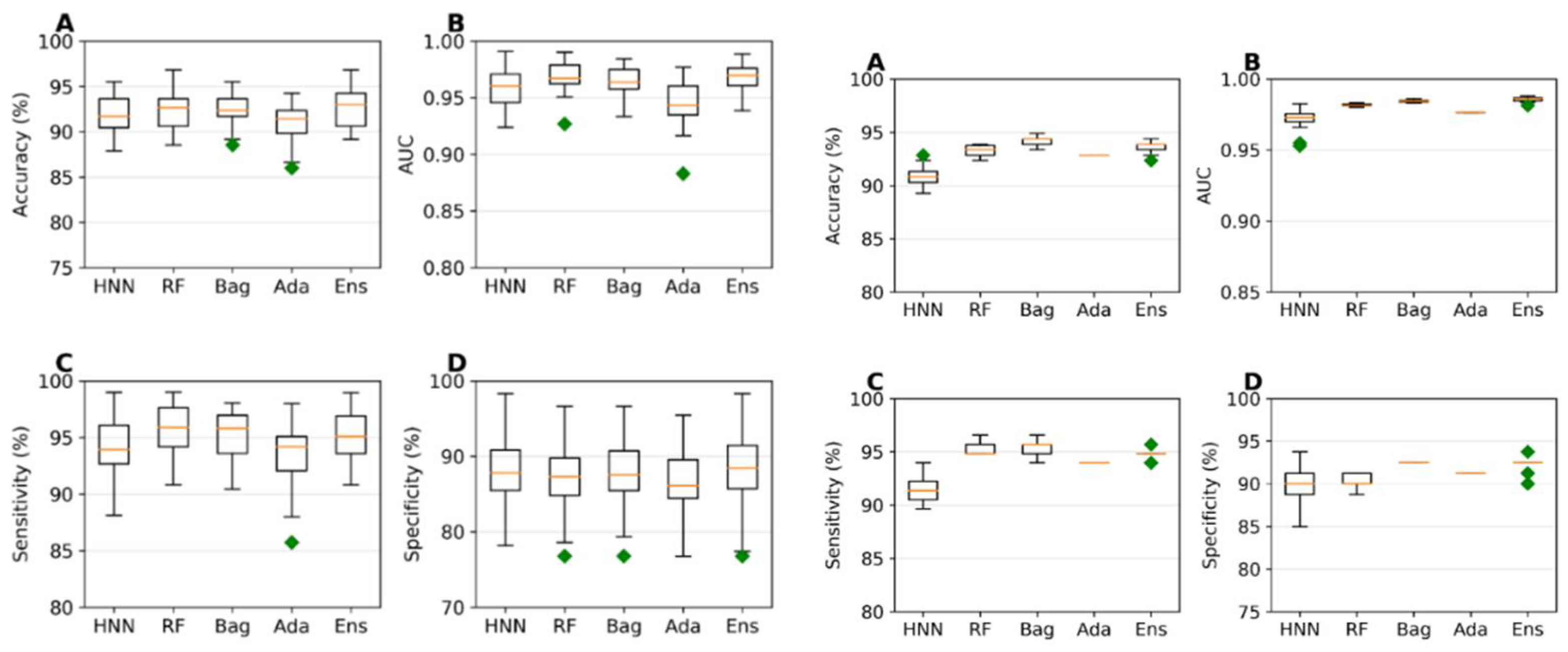
Figure 3.
a. A) Coefficient of determination (R2), B) mean squared error (MSE), and C) mean absolute error (MAE) for the data in the training set achieved by the regression models based on HNN, RF, SVR, GB, KR, DTBoost, NN and Consensus methods. b. A) Coefficient of determination (R2), B) mean squared error (MSE), and C) mean absolute error (MAE) for the validation set achieved by the regression models based on HNN, RF, SVR, GB, KR, DTBoost, NN and Consensus methods.
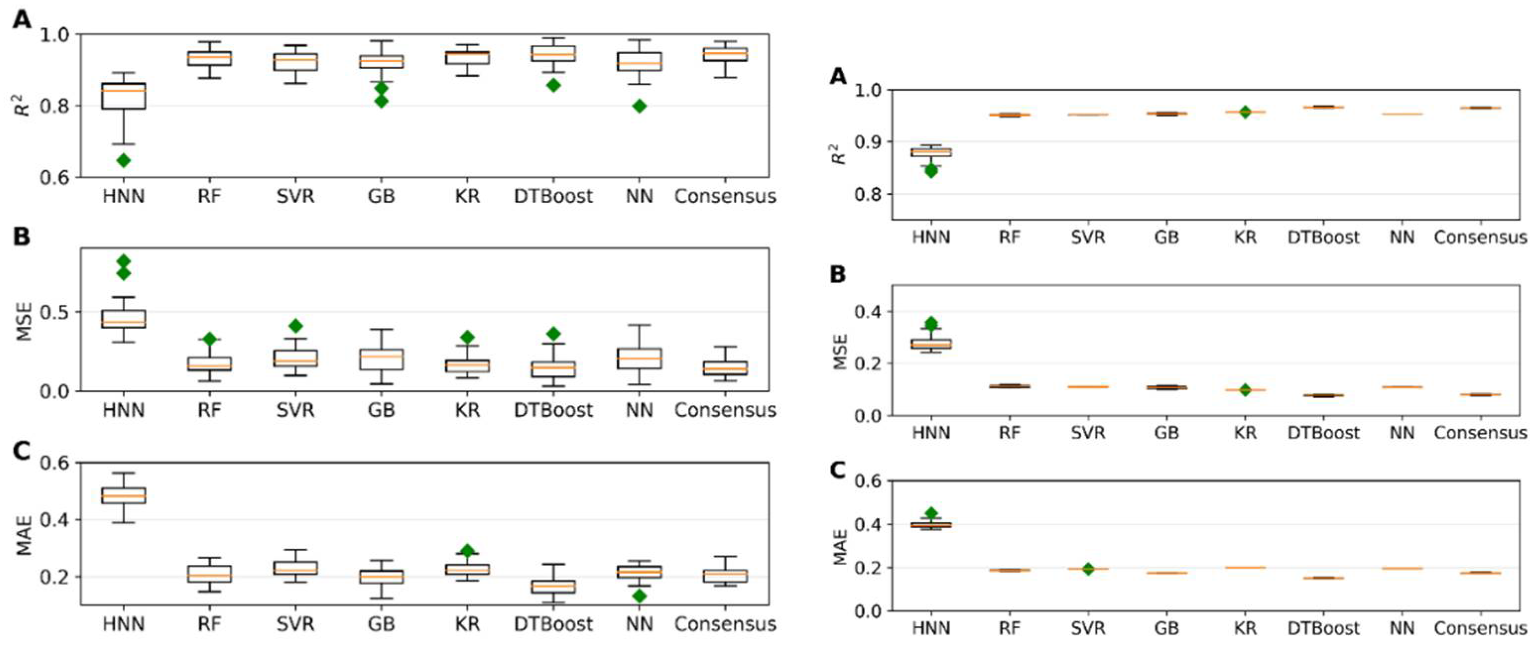
Figure 4.
a: Prediction accuracy, sensitivity, specificity, precision, and AUC for the mixture dataset I (no drug combination) with 175 random mixtures in the test set, II (with 100 drugs combinations) with 200 random mixtures in the test set, and III (with all 373 drugs combinations) with 250 random mixtures in the test set by HNN, RF, Bagging, AdaBoost and the Ensemble methods. 4b:Statistical summary of the results of HNN, RF, Bagging, AdaBoost and Ensemble methods with prediction accuracy, sensitivity, specificity, precision, and AUC for the mixture datasets IV, V, and VI are shown.
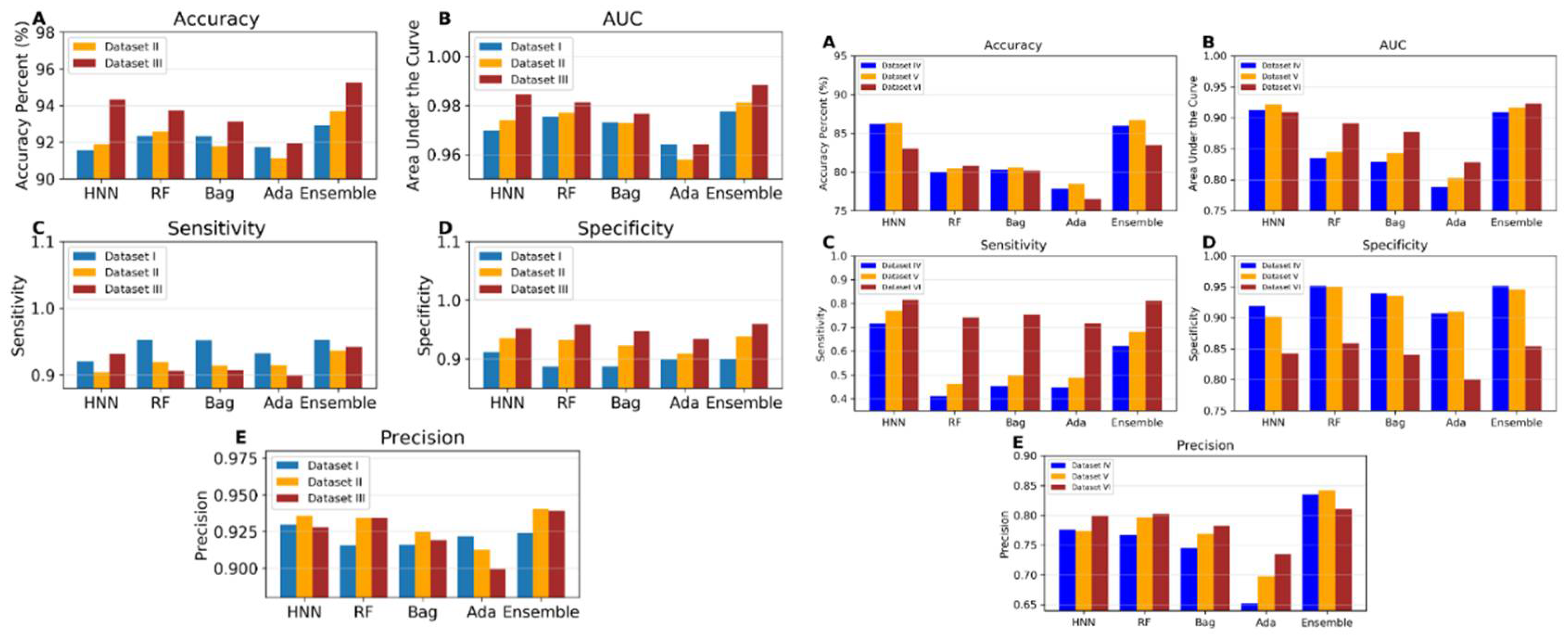
Figure 5.
Prediction accuracy, sensitivity, specificity, precision, and AUC for the compound out mixture COSet I and COSet II by HNN, RF, Bagging, AdaBoost and the Ensemble methods.
Figure 5.
Prediction accuracy, sensitivity, specificity, precision, and AUC for the compound out mixture COSet I and COSet II by HNN, RF, Bagging, AdaBoost and the Ensemble methods.
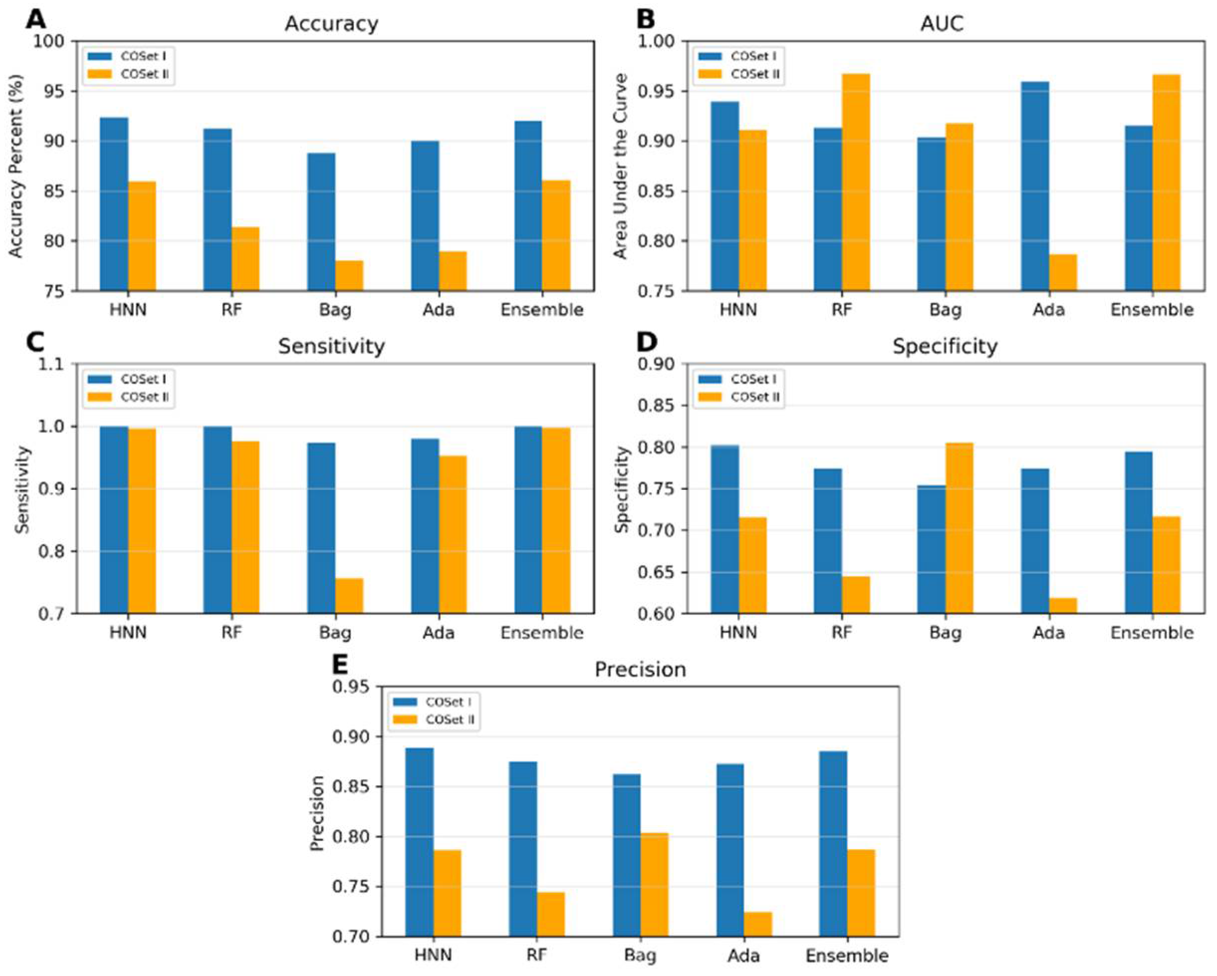
Figure 6.
Percentage of experimentally determined toxic chemicals counted a) against CPTM’s Z-score ranking of chemicals, b) counted against CPTM’s Z-score ranking obtained after adding ML (AI-HNN) score - (AI-CPTM).
Figure 6.
Percentage of experimentally determined toxic chemicals counted a) against CPTM’s Z-score ranking of chemicals, b) counted against CPTM’s Z-score ranking obtained after adding ML (AI-HNN) score - (AI-CPTM).
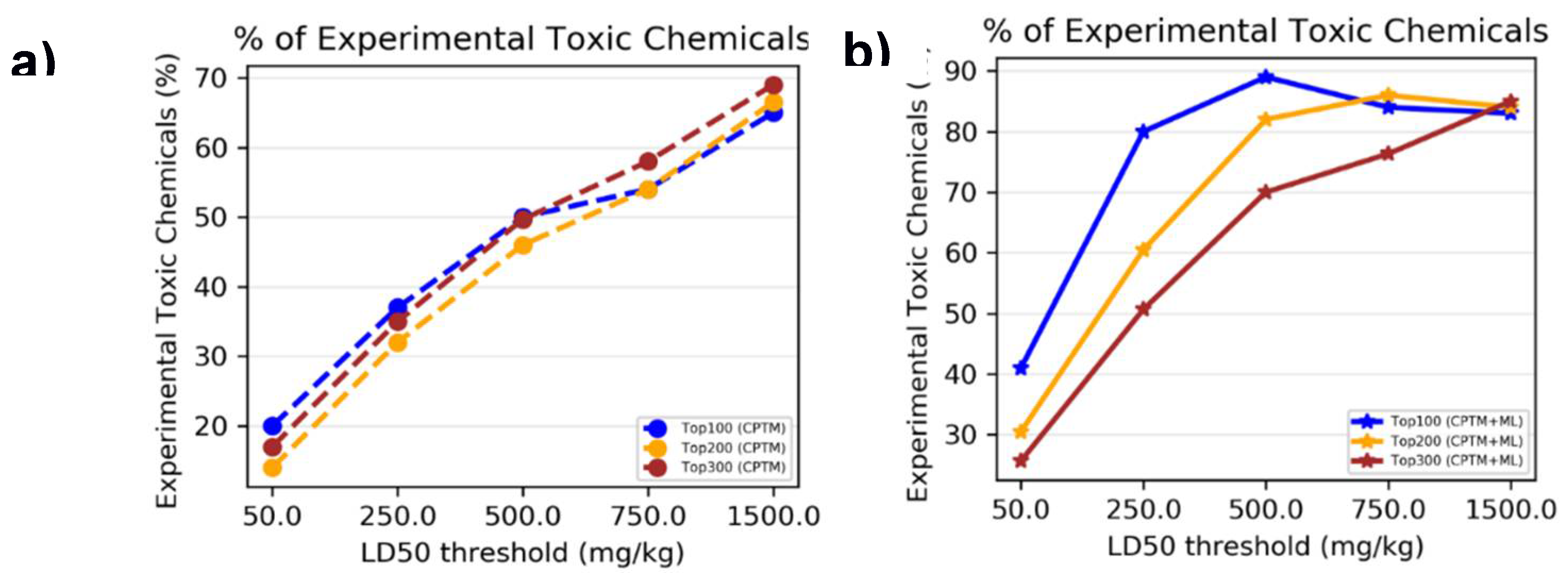
Figure 7.
a) Percentage of machine learning based predicted toxic chemicals counted against CPTM’s Z-score ranking of chemicals, b) the percentage of chemicals correctly identified as toxic at various Z-score cutoffs (e.g., top 100, 200, 300) after incorporating HNN predictions into the CPTM.
Figure 7.
a) Percentage of machine learning based predicted toxic chemicals counted against CPTM’s Z-score ranking of chemicals, b) the percentage of chemicals correctly identified as toxic at various Z-score cutoffs (e.g., top 100, 200, 300) after incorporating HNN predictions into the CPTM.
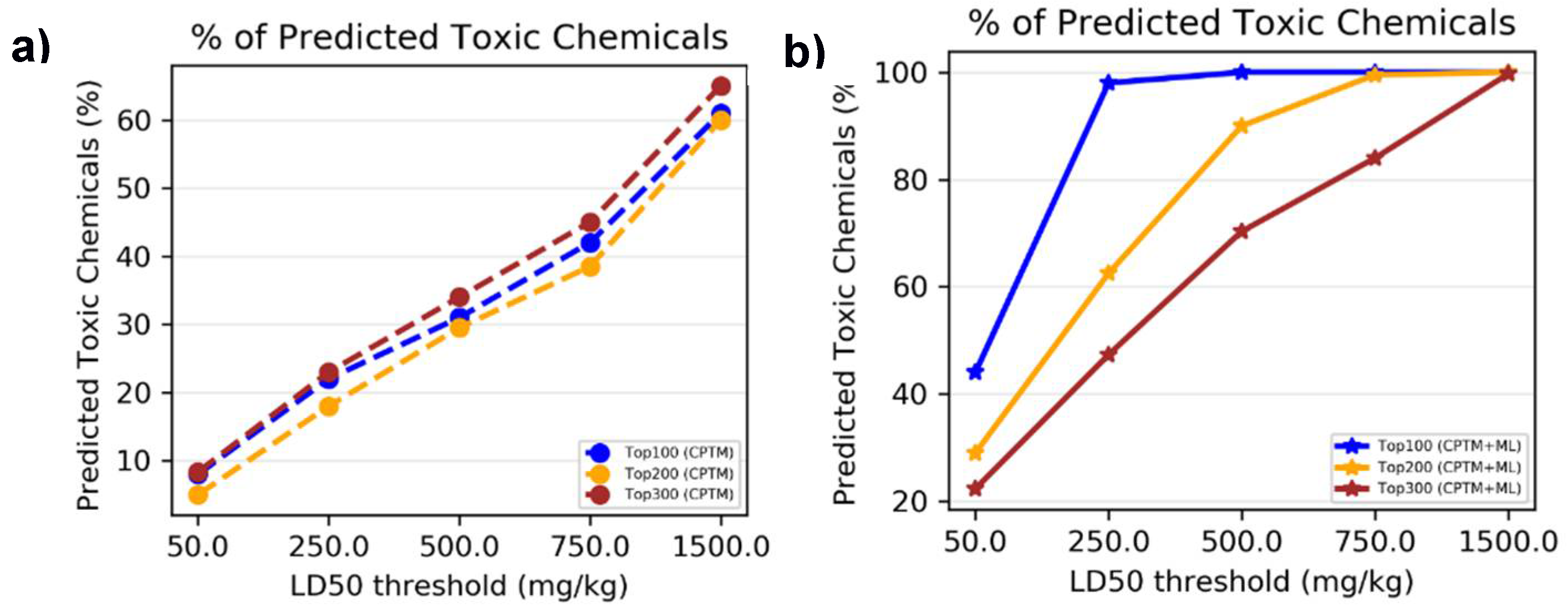
Figure 8.
a) Percentage of experimental 1s (toxic) counted against CPTM’s Z-score ranking and ranking obtained after machine learning (ML) predictions integrated into the Z-score. b) Percentage of predicted 1s counted against CPTM’s Z-score ranking and ranking obtained after machine learning (ML) predictions integrated into the Z-score.
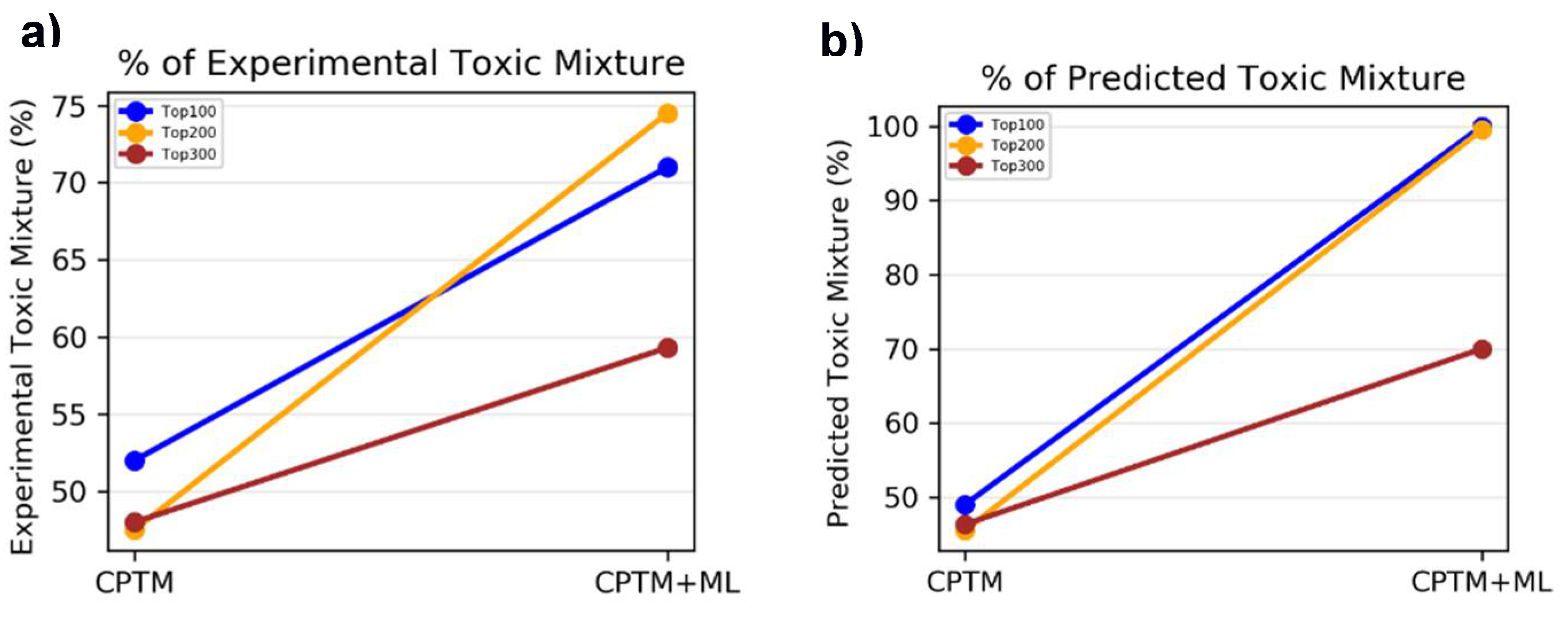
Figure 9.
Dose dependent toxicity assessment of AI-CPTM predicted chemicals (Table 2 and Table 3) as the lowest dose leading to defined here as significant developmental abnormalities at 2days after post fertilization (2 dpf) in a dose response zebrafish live assay.
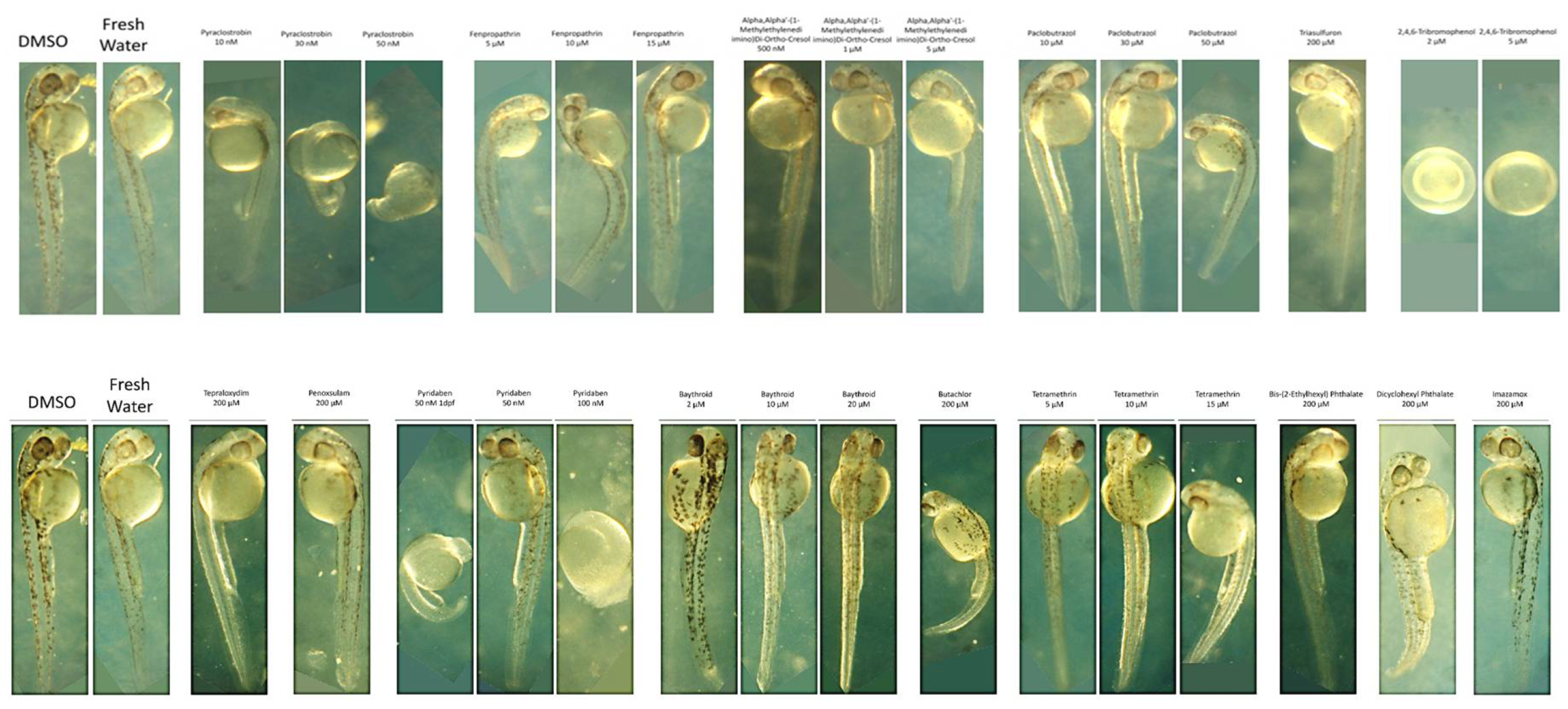
Figure 10.
Mixed chemical phenotypes and how they are scored. The mixed chemical phenotype score is the sum of the scores for the five-individual fish in a well. Two wells were treated per chemical combination and the scores are averaged for the wells. Scoring was as follows: dead = 0; severely deformed =1; deformed =2; slightly deformed = 3; and normal phenotypes = 4.
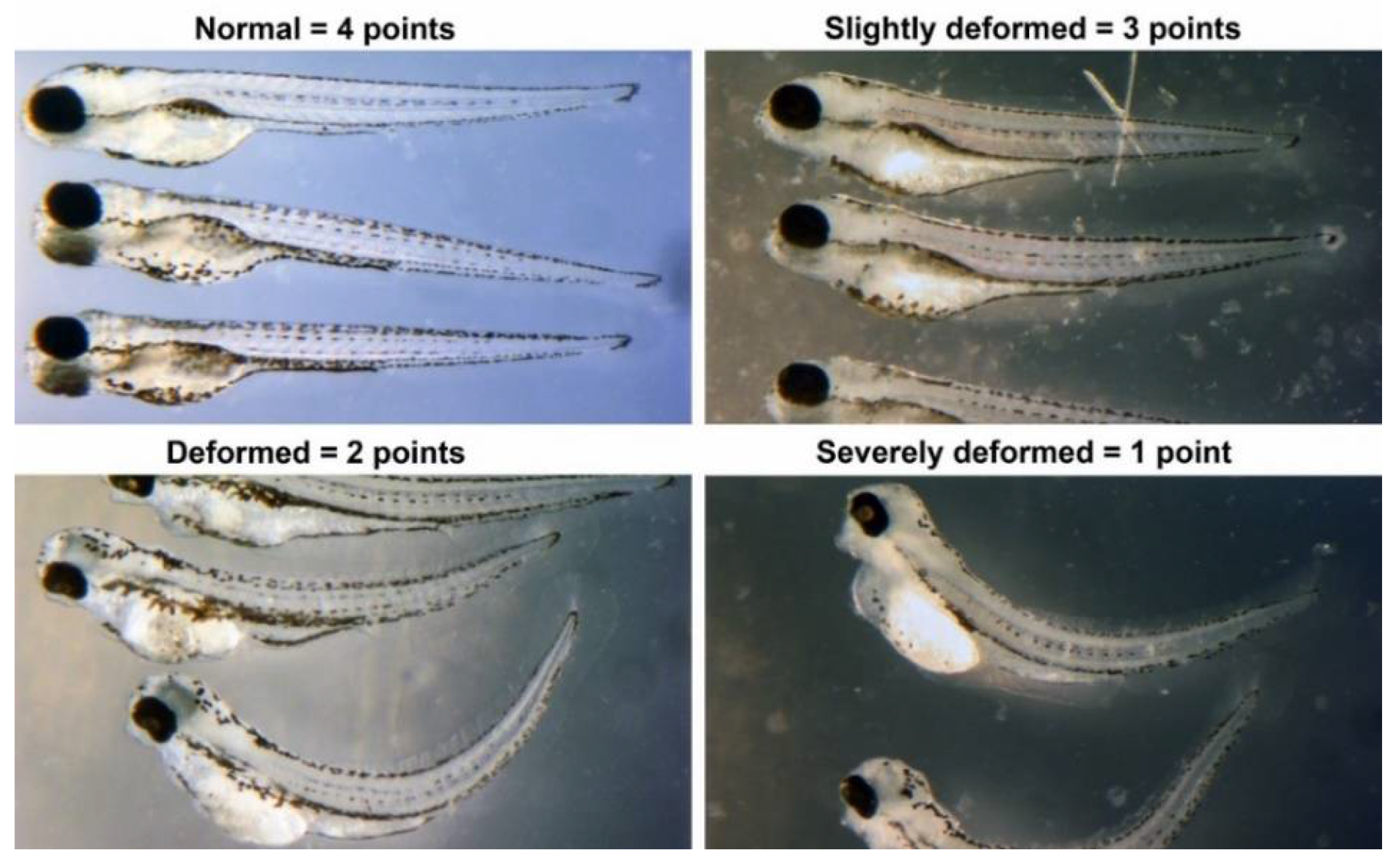
Figure 11.
The results of zebrafish toxicity studies for Panel a) selected single chemicals and Panel b) their mixture combinations. Panel A, is the toxicity data obtained from single chemical dose-response studies were used to inform the mixed chemical toxicity studies. Panel B, mixtures toxicity assessed based on the presence of significant developmental abnormalities in the embryos, with DMSO and water as control. Additionally, the outcomes regarding toxicity, developmental abnormalities, and chemical-chemical interactions are in Table 3 and Figure 9 and Figure 10. The rationale behind the selection of doses for mixture toxicity studies is detailed within the main text.
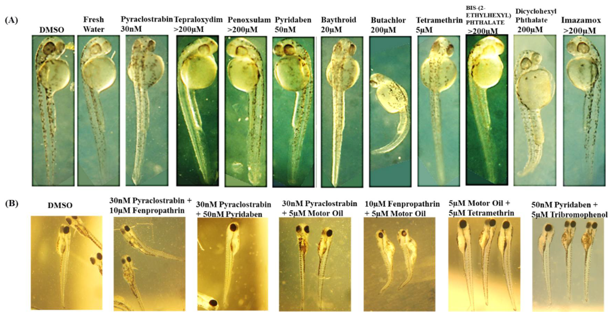
Figure 12.
Dose-response of zebrafish survival rates upon exposure to PFOA and PFOS mixtures (Table 5).
Figure 12.
Dose-response of zebrafish survival rates upon exposure to PFOA and PFOS mixtures (Table 5).
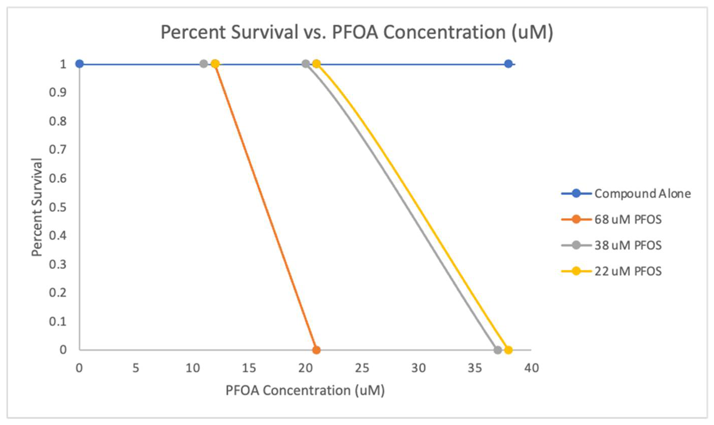

Table 2.
11 toxic chemicals for binary combination toxicity prediction.
| Chemicals | CASRN |
|---|---|
| Pyraclostrobin | 175013-18-0 |
| Fenpropathrin | 39515-41-8 |
| Alpha, alpha’-(1-methylethylenediimino)di-ortho-cresol | 94-91-7 |
| Paclobutrazol | 76738-62-0 |
| 2,4,6 -Tribromophenol | 118-79-6 |
| Pyridaben | 96489-71-3 |
| Butachlor | 23184-66-9 |
| Tetramethrin | 7696-12-0 |
| Dicyclohexyl Phthalate (DCHP) | 84-61-7 |
| Pentadecafluorooctanoic acid (PFOA) | 335-67-1 |
| Prefluorooctane sulfonic acid (PFOS) | 1763-23-1 |
Table 3.
Toxicity predictions by HNN, Random Forest, Bagging, and AdaBoost method of machine learning along with the concentration of the components for the binary mixtures of 10 chemicals listed in Table 2. Last column lists the experimental toxicity prediction.
Table 3.
Toxicity predictions by HNN, Random Forest, Bagging, and AdaBoost method of machine learning along with the concentration of the components for the binary mixtures of 10 chemicals listed in Table 2. Last column lists the experimental toxicity prediction.
| Chemical 1 | Concentration LC50 (µM) | Chemical 2 | Concentration LC50 (µM) | AI-CPTM | AI-HNN | RF | Bagging | Adaboost | Experiment (zebrafish) | Mixture chemical interaction |
|---|---|---|---|---|---|---|---|---|---|---|
| Pyraclostrobin | 0.01 | Fenpropathrin | 5 | 0 | 0 | 1 | 1 | 1 | 0 | no interaction |
| Alpha, alpha’-(1-methylethylenediimino)di-ortho-cresol (motor fuel oil) | 2.5 | 0 | 0 | 1 | 1 | 1 | 0 | no interaction | ||
| Paclobutrazol | 50 | 1 | 1 | 1 | 1 | 1 | 0 | inconclusive | ||
| 2,4,6 -Tribromophenol | 2 | 1 | 1 | 1 | 1 | 1 | 1 | inconclusive | ||
| Pyridaben | 0.05 | 0 | 1 | 1 | 1 | 1 | 0 | inconclusive | ||
| Butachlor | 100 | 1 | 1 | 0 | 0 | 0 | 1 | no interaction | ||
| Tetramethrin | 5 | 1 | 0 | 0 | 1 | 1 | 1 | inconclusive | ||
| Dicyclohexyl Phthalate (DCHP) | 100 | 1 | 0 | 1 | 1 | 0 | 1 | inconclusive | ||
| Fenpropathrin | 5 | Alpha, alpha’-(1-methylethylenediimino)di-ortho-cresol | 2.5 | 1 | 1 | 1 | 0 | 1 | 1 | additive |
| Paclobutrazol | 50 | 1 | 1 | 1 | 1 | 1 | 1 | additive | ||
| 2,4,6 -Tribromophenol | 2 | 1 | 1 | 1 | 1 | 1 | 1 | additive | ||
| Pyridaben Pestanal | 0.05 | 1 | 1 | 1 | 1 | 1 | 0 | no interaction | ||
| Butachlor | 100 | 1 | 1 | 0 | 0 | 0 | 1 | additive | ||
| Tetramethrin | 5 | 1 | 1 | 1 | 1 | 1 | 1 | synergistic | ||
| Dicyclohexyl Phthalate (DCHP) | 100 | 1 | 1 | 1 | 1 | 0 | 1 | synergistic | ||
| Alpha, alpha’-(1-methylethylenediimino)di-ortho-cresol (motor oil) | 2.5 | Paclobutrazol | 50 | 1 | 1 | 1 | 1 | 1 | 1 | additive |
| 2,4,6 -Tribromophenol | 2 | 1 | 1 | 1 | 1 | 1 | 1 | additive | ||
| Pyridaben Pestanal | 0.05 | 0 | 0 | 0 | 1 | 1 | 0 | inconclusive | ||
| Butachlor | 100 | 0 | 0 | 1 | 0 | 0 | 1 | additive | ||
| Tetramethrin | 5 | 0 | 0 | 0 | 0 | 1 | 0 | no interaction | ||
| Dicyclohexyl Phthalate (DCHP) | 100 | 0 | 0 | 0 | 0 | 0 | 0 | no interaction | ||
| Paclobutrazol | 50 | 2,4,6 -Tribromophenol | 2 | 0 | 0 | 1 | 1 | 1 | 0 | no interaction |
| Pyridaben | 0.05 | 1 | 1 | 1 | 1 | 1 | 1 | additive | ||
| Butachlor | 100 | 1 | 1 | 1 | 1 | 1 | 1 | synergistic | ||
| Tetramethrin | 5 | 0 | 0 | 1 | 0 | 1 | 0 | additive | ||
| Dicyclohexyl Phthalate (DCHP) | 100 | 1 | 1 | 1 | 0 | 1 | 0 | additive | ||
| 2,4,6 -Tribromophenol | 2 | Pyridaben Pestanal | 0.05 | 1 | 1 | 1 | 1 | 1 | 0 | no interaction |
| Butachlor | 100 | 1 | 1 | 0 | 0 | 0 | 1 | synergistic | ||
| Tetramethrin | 5 | 1 | 1 | 1 | 1 | 1 | 1 | additive | ||
| Dicyclohexyl Phthalate (DCHP) | 100 | 1 | 1 | 1 | 0 | 0 | 1 | no interaction | ||
| Pyridaben | 0.05 | Butachlor | 100 | 1 | 1 | 1 | 1 | 1 | 1 | synergistic |
| Tetramethrin | 5 | 1 | 1 | 1 | 1 | 0 | 0 | inconclusive | ||
| Dicyclohexyl Phthalate (DCHP) | 100 | 1 | 1 | 1 | 1 | 0 | 0 | inconclusive | ||
| Butachlor | 100 | Tetramethrin | 5 | 1 | 1 | 1 | 0 | 1 | 1 | synergistic |
| Dicyclohexyl Phthalate (DCHP) | 100 | 1 | 1 | 1 | 1 | 1 | 1 | synergistic | ||
| Tetramethrin | 5 | Dicyclohexyl Phthalate (DCHP) | 100 | 1 | 1 | 1 | 1 | 1 | 1 | inconclusive |
| Prefluorooctane sulfonic acid (PFOS) | 53 | Pentadecafluorooctanoic acid (PFOA) | 187.5 | 1 | 1 | 1 | 1 | 1 | 1 | synergistic |
Table 4.
Toxicity of PFOS and PFOA in zebrafish embryos. The LD50 and EC50 concentrations for zebrafish embryos exposed to PFOS and PFOA at 2days post fertilization for one day at 33°C. LD50 defined as the lethal dose resulting in the death of 50% of the embryos. EC50 is defined as the effective dose where 50% of the embryos display any abnormality, including bent body axis, edema, cloudy tissue, developmental delay.
| Compound | LD50 | EC50 |
|---|---|---|
| PFOS | 53 µM | 11 µM |
| PFOA | 187.5 µM | 29.5 µM |
Table 5.
PFOS and PFOA mixture LD50 concentrations. The LD50 for PFOA when mixed with PFOS, were determined at three PFOS concentrations.
Table 5.
PFOS and PFOA mixture LD50 concentrations. The LD50 for PFOA when mixed with PFOS, were determined at three PFOS concentrations.
| Concentration of PFOS Present (µM) | 68 µM PFOS | 38 µM PFOS | 22 µM PFOS |
| LD50 (added PFOA concentration (µM) | 16.5 µM PFOA | 29 µM PFOA | 29.5 µM PFOA |
Disclaimer/Publisher’s Note: The statements, opinions and data contained in all publications are solely those of the individual author(s) and contributor(s) and not of MDPI and/or the editor(s). MDPI and/or the editor(s) disclaim responsibility for any injury to people or property resulting from any ideas, methods, instructions or products referred to in the content. |
© 2024 by the authors. Licensee MDPI, Basel, Switzerland. This article is an open access article distributed under the terms and conditions of the Creative Commons Attribution (CC BY) license (http://creativecommons.org/licenses/by/4.0/).
Copyright: This open access article is published under a Creative Commons CC BY 4.0 license, which permit the free download, distribution, and reuse, provided that the author and preprint are cited in any reuse.


