Submitted:
30 May 2024
Posted:
31 May 2024
You are already at the latest version
Abstract
The present paper proposes an accurate characterization of a NACA 23012 airfoil at near stall conditions at a Reynolds number $Re=3\cdot 10^5$. In light of the unavoidable limits of which experiments suffer near the stall regime both in terms of effective two--dimensionality and data portability across different research groups, the present characterization is performed through high fidelity numerical simulations. Taking advantage of the local discontinuous Galerkin (LDG) LES solver, implemented in the open source library \textit{FEMilaro}, the airfoil behavior is investigated ranging from $\alpha=5^{\circ}$ to $17^{\circ}$, with a peculiar focus for $\alpha \ge 10^{\circ}$. Accuracy of the found results is ensured both from the realistic and accurate reconstructed flow physics and by means of a proper comparison with existing experimental data. Then, a reliable numerical baseline is obtained for any future investigation involving a NACA 23012 airfoil at $Re=3 \cdot 10^5$. The future study of the actual research group will be a parallel BVI analysis, but results are completely extendable as they are to any other research.
Keywords:
NACA 23012
; LES
; discontinuos Galerkin
; BVI
1. Introduction
Rotary wing aircraft are characterised by a very complex aerodynamics. In fact, the motion of the lifting surfaces produces complex wakes, which shape is strongly dependent on the flying condition, see e.g. [1,2]. The presence of wakes with complicated geometries generates a plenty of aerodynamic interactions between the various components of the aircraft. According to the flying condition, a relevant interaction that may affects all these possible configurations is the result of the collision of the tip vortex generated by a blade against another blade of the rotor. This phenomenon, said blade vortex interaction (BVI), plays an important role in modern rotary wing aircraft design. In fact, BVI occurrences both generate meaningful acoustic waves and sudden local variations of the lift produced by the stricken blade [3]. Among the several different ways a BVI event can occur a meaningful one is the so–called parallel BVI, where the axis of the tip vortex is locally parallel to the spanwise direction of the blade. While other kinds of BVI events involve almost a single slice of the blade, the parallel BVI acts on a larger portion of the blade due to the peculiar alignment between the vortex and the blade axes. Then, parallel BVI potentially induces larger variations in the overall aerodynamic loads. Recently, there appear two interesting studies concerning parallel BVI events for a NACA 23012 airfoil at : a high fidelity numerical study at [4] and an extensive experimental analysis [5]. In particular, this experimental study highlights how the parallel BVI is capable to generate a meaningful variation of the pressure distribution on the suction side, that may triggers the stall of the airfoil when it operates very near to the stall condition.
This experimental investigation provides an interesting global description of the phenomenon. However, the full detail of the intrinsic phenomenology that rules the blade vortex interaction is hardly ever achievable by means of a wind tunnel test. Of course, experimental data are essential for the comprehension of this aerodynamic interaction as for the validation of any numerical tool, but it is evident that an accurate numerically reconstructed flow field easily provides information that are otherwise barely obtainable experimentally. For example, this is the case of the skin friction coefficient distribution over the airfoil and of the details of the interaction between the impinging vortex and the turbulent structures inside the suction side boundary layer. This surely motivates the interest towards high fidelity numerical simulations, but it is not the only reason. In fact, even if namely , every wind tunnel experiment is not completely two-dimensional, especially near the stall. As important implication data are, up to a certain level, wind tunnel dependent. This is rather evident by the collection of curves in Figure 1 for a NACA 23012 airfoil in clean configuration and in the range – . The data scattering near the stall condition surely exceeds whatever Reynolds dependence, that is expected small inside the considered range. Likely, after proper validation, high fidelity numerical studies are also more portable between different research groups.
The present paper provides a high fidelity numerical characterization of the clean configuration of NACA 23012 airfoil at for , with a peculiar focus for , i.e., around the stall regime. This study is intended as the first step towards the numerical simulation of parallel BVI events, that would be a valuable addition to the work [5]. Note that such future perspective is not redundant with the study [4], since it would be performed at higher and, in light of [5], more meaningful angles of attack. This final goal determines the selected airfoil and operative conditions. However, this work hopefully is more general, providing a valid numerical reference for the clean NACA 23012 for other researchers interested to any other possible study on this airfoil. Reference that, up to the authors knowledge, is not already available for NACA 23012 at these, or comparable, operative conditions.
2. Materials and Methods
In order to ensure high accurate results, a LES approach has been selected. The present simulations are run using the local discontinuous Galerkin (LDG) LES solver implemented inside the open source FEMilaro library [11], written according to the latest Fortran and MPI standards. This library has been selected by virtue of the highly parallelizable nature of LDG schemes [12], that allow very efficient implementations.
2.1. Mathematical Model
The selected solver approaches the Navier–Stokes equations in their compressible form. The mathematical formulation behind this solver is well reported in [13] but, for the sake of completeness, its main aspects are briefly recalled here. In particular, according to a common practice in compressible LES, equations are filtered supposing the commutation between the LES filter and the derivatives. Indicating as the LES filter and the Favre decomposition associated to and defined as [14], the compact form (1) for the filtered Navier–Stokes equation is obtained.
Here, , and , where is the density, the velocity, e the internal energy and T the temperature. The notation and means and respectively. Note that the system (1) is written as a system of first order PDEs, since the LDG discretization requires this kind of rewriting [15,16].
The terms and are the convective (or eulerian) and the diffusive (or viscous) fluxes classically defined in the Navier-Stokes equations, but evaluated with filtered variables. Instead, is the subgrid flux and contains all the terms that requires a model. In particular, its expression is reported in equation (2).
In equation (2), is the subgrid stress tensor, the subgrid heat flux and the subgrid turbulent diffusion flux.
Among the different closures proposed inside FEMilaro, the anisotropic dynamic model originally formulated in [17] and extended to the compressible case in [13] is adopted to model the term (2). The details of the mathematical formulation are not reported here since they are not the main focus of the present work, but a couple of comments on the properties of this model are appropriate. In particular, this turbulent closure is both anisotropic and based on a revisitation of Germano’s dynamic procedure. Then, it is capable to capture small scales anisotropicity and it is self–tailored on the local characteristics of the flow, being able to describe also backscatter phenomena. In light of these theoretic features and of the validation with FEMilaro library in [13,18], this model is assumed accurate enough for the present study. Note that the current implementation of the model presents a small change with respect to its original formulation. Indeed, the filter size is not explicitly defined but it is included in the model coefficients determined by the dynamic procedure, as in [19].
2.2. Simulation Setup
The computational domain is obtained from the extrusion in the z direction for a distance of a C–type domain defined in the plane. The two–dimensional geometry is reported in Figure 2 and it is parameterized in R frontal radius and L wake length. The airfoil trailing edge is located at and it is put at the angle of attack through a rotation around this point. The airfoil chord is . Parameters R, L and are selected combining the results of some fast preliminary independence tests, which results are reported in Section 3.1, with available literature concerning high fidelity numerical simulations of airfoils, e.g., [20,21,22,23]. The final choice is reported in Table 1.
On this domain, a hybrid structured–unstructured mesh of tetrahedra is build through the open source mesher GMSH. The structure portion around the airfoil is created building a structured of hexahedra, composed by 25 layers of 225 elements in the plane and repeated 8 times in the z direction. Each of these hexahedra is divided into 6 tetrahedra based on the hexahedron’s vertices. The resulting overall grid consists in 365,938 thetraedra. The construction strategy is identical for all the angles of attack considered in this work. A sketch of the structured portion is reported in Figure 3 for .
Concerning boundary conditions, a Dirichlet datum equal to the free stream values is enforced on all the outer boundaries except on the sides perpendicular to the spanwise direction, where periodic conditions are imposed. The airfoil surface is modeled as an isothermal wall with no slip condition on the velocity. Instead, initial conditions are the default ones of FEMilaro solver, i.e., a uniform flow equal to and damped around the airfoil according to a Gaussian function, in order to ensure the no slip condition still from the first time steps.
2.3. Simulation Strategy
The simulation strategy consist in letting the simulation to evolve from the initial conditions to a statistically steady state regime. Then, this state is observed over a statistically meaningful time interval and the main quantities of interest are acquired. In this way, data mean tangential and fluctuating velocity profiles, skin friction coefficient and aerodynamic coefficients are collected.
By a technical viewpoint, all the simulations of this work are performed with a uniform polynomial distribution of degree . This results into an overall number of degree of freedom of per simulation. Moreover, a time step is employed to satisfy the condition in the whole domain for the entire duration of the simulations. This choice guarantees a maximum Courant number of .
Simulations are run exploiting 2048 parallel threads on AMD® Zen 2 EPYC™ 7H12 CPUs on Karolina, MeluXina and Discoverer supercomputers belonging to the EuroHPC JU consortium. In details, runs on Karolina and MeluXina clusters are executed using 2048 physical cores, while computations on Discoverer cluster take advantage of hyperthreading, running 2048 processes on 1024 physical cores without any meaningful time overhead.
3. Results
3.1. Preliminary Tests
The preliminary tests consists in the comparison between the first time instant of a set of ILES simulation at and variable R. This peculiar angle of attack is selected since it is one of the points associated to the largest uncertainty in terms of and , as emerged looking at Figure 1. Then, this condition is the one requiring the best possible simulation.
These tests are performed on the time interval , that it is not enough to reach a statistically steady state regime, as evidently reported from Figure 4.
This is a conscious choice, since the aim is to perform computationally cheap preliminary tests, but requires a careful comparison between the data. The absence of a final state implies that there is no regime value to compare across the tests. To avoid the comparison of pointwise values, that are rather meaningless during a transient with turbulence, the equivalence of the time histories is evaluated comparing the mean value of the difference between the time histories. Moreover, since a compressible solver is used, data must be compared after the pressure wave generated by the boundary conditions at reaches the airfoil. Of course, the change in the grid size implies boundary conditions are felt for the first time at different time instants in the different simulations. This fact is well depicted in Figure 4: after the violent oscillations in the lift coefficient, expected from the inviscid theory and that represents the first phase of the airfoil startup [24], there appear a negative peak generated by the boundary pressure wave at a location that is R dependent. Then, data must be compared at least after . Results of the comparison are reported in Table 2 for .
3.2. Simulations
In the present work six different angles of attack are considered: five around the stall regime, that are , , , , , and one in the linear range of the curve, at . This latter case might appear out of the scope of this work. However, the purpose of this low simulation consists in offering a more robust validation of the results.
All the simulations are run according to the simulation strategy proposed in Section 2.3. Note that each single run requires a small ad hoc customization. In fact, the growing flow unsteadiness due to the increase in the angle of attack makes the observation interval of the final statistically steady state simulation-dependent. Simulations at the lowest values of require a much shorted acquisition window. Instead, the settling time to reach this final regime is roughly constant for all the tested angles.
The instantaneous flow fields in the steady state regime are reported in Figure 5 according to the angle of attack. At the flow is completely attached and exhibits a thin boundary layer with a low turbulence level. Increasing the angle of attack, a larger and larger low velocity region appears at the trailing edge from , indicating an incoming trailing edge stall. The same information is deduced by the progressive thickening of the boundary layer. Moreover, as evident by the leading edge detail in Figure 6, the transition point moves progressively towards the front portion of the airfoil. There, the transition is triggered by a laminar separation bubble (LSB), especially at high values of .
The qualitative description deduced from the the flow fields is supported from the analysis of the velocity profiles in Figure 7. Figure 7 reports the mean tangential velocity profiles extracted along lines normal to the airfoil surface. The chord position of these lines is reported in Table 3, while Figure 8 offers a their sketch at .
The analysis of Figure 7 confirms a progressively larger mean trailing edge separation starting for . Moreover, also the first velocity profile exhibits a recirculation region, confirming the presence of a laminar separation bubble near the leading edge. As already observed in Figure 6, this LSB is stronger higher the angle of attack is. The presence of such aerodynamic structure is expected at these operative conditions [25] and also low fidelity simulations through solvers as XFOIL exhibit a LSB for NACA 23012 at . The presence of the laminar separation bubble, as well as of the trailing edge separation, is confirmed by the skin friction coefficient reported in Figure 9. In fact, the are negative regions of both on the front and at the rear of the airfoil. These regions are larger higher is, confirming what observed about profiles 1 and 10.
It is also of interest the analysis of some turbulent quantities, as the resolved turbulent fluctuations. Then, some profiles for the fluctuating quantities are investigated, where and denotes the time average. With reference to the same chord positions used for the mean velocity profiles and reported in Table 3, the profiles for , and are reported in Figure 10 for the angles of attack in Figure 9. Also the lower value of is added to provide a better comparison.
At the position of the laminar separation bubble the highest fluctuations are observed both in terms of and , even if they are limited in a small region near the wall. Also the largest negative value of is observed at this location. Note that a negative value of is connected to the production of turbulent kinetic energy. Then, the LSB is effectively triggering transition from the laminar to turbulent boundary layer, generating the most part of the turbulent kinetic energy. Moreover, note how this production is larger higher the angle of attack is. Comparing this information with Figure 9, it is clear that a stronger LSB introduces more turbulent kinetic energy in the boundary layer. Moving along the suction side, the absolute values of the fluctuations are smaller and smaller near the wall, but it is evident how, especially near the trailing edge, these fluctuations are no longer limited to the near wall region. After the LSB the turbulent production progressively decreases, while larger structures progressively appears. In practice, small turbulent structures near the leading edge are transported by the flow towards the leading edge and during this transport redistribution mechanisms make them grow. As expected, higher the angle of attack is stronger this phenomenon is.
Concerning the characterization of the global behavior of NACA 23012, it is provided by means of lift and drag coefficients. Figure 11 presents and numerical curves compared with experimental data from [6,7,8,9,10]. Numerical coefficients are averaged in time over an appropriate time interval. Data are summarized in Table 4.
Remarkably, the lift coefficient data demonstrate the presence of a very smooth stall. The stall is a trailing edge separation and it is not triggered by the blow up of the laminar separation bubble. The LSB exhibits a stable behaviour across all the considered angles of attack, suggesting that its presence is only detrimental for the maximum lift coefficient [25] but does not play a role in the stall mechanism in the light stall region.
4. Discussion
In order to validate the present results, the comparison with experimental data in Figure 11 is essential. However, the numerical curve in Figure 11 agrees only with some experimental sets of measurements. Since the evident scattering of the experimental data this is rather expected, but complicates the validation of the current results.
In the linear range, all experiments almost agree one with the other except the one of Dent et al. [7]. Looking at this peculiar set of data, the slope is smaller. This reduction likely is related to a aerodynamic effect as non negligible tip vortices. Moreover, the presence of tip vortices that reduce the effective angle of attack of the airfoil justifies also the high stall angle, around , higher than in all the other measures.
Excluding this set of data, the numerical result at is in good agreement with all the measurements. Instead, for higher angles, i.e., , the numerical estimations are confirmed only by Ashender et al. [6] and Tenzin [10]. In this case, note that the deviation from Jacobs et al. [8] and Rivero et al. [9] is mainly due to a different behavior outside the linear range. Observe that the deviation from the linear range usually takes place at the point where viscous effects start playing an important role and separation begins occurring. In these conditions, experiments can be affected by the peculiar characteristics of the wind tunnel where they are performed. The larger scales of the flow structures that appear approaching the stall potentially are more sensitive to the finite size of the test chamber. Moreover, the interaction between the boundary layer on the wind tunnel walls and the one on the airfoil alters the flow on the model tips in a way that surely is wind tunnel dependent. Furthermore, this interaction is reasonably larger thicker the airfoil boundary layer is, then near the stall condition. The lower predictions in terms of and stall angle of Jacobs et al. and Rivero et al. are attributed to wind tunnel effect as the just discussed ones. Since the full detail concerning the test strategies is not available this is only an hypothesis, but a reasonable one.
Then, consider the two remaining measurements. Tenzin data confirm the LES maximum lift coefficient, since the experimental datum is and the numerical prediction is . However, Tenzin suggests an earlier stall, around . On the other hand, Ashender reports a similar stall, both in terms of smoothness and angle of maximum lift coefficient, but a lower of . However, this data is provided with a confidence interval of and the LES estimation is quite near to the upper bound of this interval. In addition, the previous discussion on Jacobs and Rivero data suggests that a slightly lower experimental prediction of with respect to the perfectly and ideal LES environment is reasonable.
In light of these considerations, the good agreement of numerical data with Tenzin and, particularly, with Ashender measures suggests the correctness of the found results. Then, a numerical baseline is available for future studies involving a NACA 23012 airfoil at the operative conditions of . The presence of these accurate numerical flow fields is a valuable addition to experiments, since it provides a reference not only for lift and drag coefficients, but also for the details of the flow physics.
Author Contributions
Conceptualization, A.A., G.G. and P.V; methodology, A.A. and P.V.; software, P.V.; validation, P.V.; formal analysis, A.A, G.G. and P.V; investigation, A.A. and P.V.; data curation, G.G.; writing—original draft preparation, P.V.; writing—review and editing, A.A. and G.G; visualization, A.A., P.V. All authors have read and agreed to the published version of the manuscript.
Funding
This research received no external funding.
Institutional Review Board Statement
Not applicable.
Data Availability Statement
Data are available upon request on the authors.
Acknowledgments
We acknowledge EuroHPC Joint Undertaking for awarding us access to EuroHPC supercomputer Karolina hosted by IT4Innovations National Supercomputing Center at VSB – Technical University of Ostrava, Czech Repubblic, EuroHPC supercomputer MeluXina hosted by LuxProvide at LuxConnect’s Data Center DC2, Luxembourg and EuroHPC supercomputer Discoverer hosted by PetaSC Bulgaria at Sofia Tech Park, Bulgaria.
Conflicts of Interest
The authors declare no conflicts of interest.
Abbreviations
The following abbreviations are used in this manuscript:
| BVI | Blade vortex interaction |
| CFL | Courant-Friedrichs-Lewy |
| DNS | Direct numerical simulation |
| ILES | Implicit LES |
| LDG | Local discontinuous Galerkin |
| LES | Large eddy simulation |
| LSB | Laminar separation bubble |
| PDE | Partial differential equation |
References
- Ananthan, S. Analysis of Rotor Wake Aerodynamics During Maneuvering Flight Using a Free-Vortex Wake Methodology. PhD thesis, University of Maryland, College Park, Department of Aerospace Engineering, 2006.
- Egolf, T.A.; Landgrebe, A.J. Helicopter Rotor Wake Geometry and Its Influence in Forward Flight. Technical report, NASA contractor report 3726, 1983. Volume I, Generalised Wake Geometry and Wake Effect on Rotor Airloads and Performance, and Volume II, Wake Geometry Charts.
- Leishman, J.G. Principles of Helicopter Aerodynamics, 2nd ed.; Cambridge University Press: 32 Avenue of the Americas, New York, NY 10013-2473, USA, 2006. [Google Scholar]
- Colli, A.; Abbà, A.; Gibertini, G. Experimental and Numerical Study of Parallel Blade-Vortex Interaction. In Proceedings of the 48th European Rotorcraft Forum, September 2022. Paper 096.
- Colli, A.; Zanotti, A.; Gibertini, G. Wind Tunnel Experiments on Parallel Blade–Vortex Interaction with Static and Oscillating Airfoil. Fluids 2024, 9, 111. [Google Scholar] [CrossRef]
- Ashender, R.; Lindberg, W.; Martwitz, J.D. Two-dimensional NACA 23012 Airfoil Performance Degradation by Super Cooled Cloud, Drizzle, and Rain Drop Icing. In Proceedings of the AIAA 34th Aerospace Sciences Meeting and Exhibit, January 1996. AIAA 96-0870.
- Dent, J.; Robson, J.; Basso, A.; Ellin, A.; Prakash, A.; Hamad, F. Computational Study of Aerodynamic Performance and Flow Structure Around NACA 23012 Wing. International Journal of Aerodynamics 2019. [Google Scholar] [CrossRef]
- Jacobs, E.N.; Sherman, A. Airfoil Section Characteristics as Affected by Variations of the Reynolds Number. Technical report, NACA report 586, 1937.
- Rivero, A.E.; Fournier, S.; Manolesos, M.; Cooper, J.E.; Woods, B. Wind Tunnel Comparison of Flapped and FishBAC Camber Variation for Lift Control. In Proceedings of the AIAA Scitech 2020 Forum, session Morphing Rotor Blades, January 2020. AIAA 2020-1300.
- Tenzin, C. Experimental Investigation of Dynamic Roughness as an Aerodynamic Flow Control Method. Master’s thesis, The Pennsylvania State University, Department of Aerospace Engineering, 2010.
- FEMilaro Fortran/MPI library. Open source code. Available online: https://bitbucket.org/mrestelli/femilaro/wiki/Home (accessed on 26 May 2024). A more recent version of the code is available upon request to the authors.
- Baggag, A.; Atkins, H.; Keyes, D. Parallel Implementation of the Discontinuous Galerkin Method. Technical Report 99-35, ICASE, 1999. NASA Contractor Report 1999-209546.
- Abbà, A.; Bonaventura, L.; Nini, M.; Restelli, M. Dynamic Models for Large Eddy Simulation of Compressible Flows with a High Order DG Method. Computers and Fluids 2015, 122, 209–222. [Google Scholar] [CrossRef]
- Favre, A.J. The Equations of Compressible Turbulent Gases. Technical Report 1, Institut de mecanique statistique de la turbulence, Marseille, France, 1965. Annual summary report for Contract AF 61 (052)-772, Air Force office of scientific research.
- Bassi, F.; Rebay, S. A High-Order Accurate Discontinuous Finite Element Method for the Numerical Solution of the Compressible Navier–Stokes Equations. Journal of Computational Physics 1997, 131, 267–279. [Google Scholar] [CrossRef]
- Cockburn, B.; Shu, C.W. The Local Discontinuous Galerkin Method for Time-Dependent Convection-Diffusion Systems. SIAM Journal on Numerical Analysis 1998, 35, 2440–2463. [Google Scholar] [CrossRef]
- Abbà, A.; Cercignani, C.; Valdettaro, L. Analysis of Subgrid Scale Models. Computers and Mathematics with Applications 2003, 46, 521–535. [Google Scholar] [CrossRef]
- Abba, A.; Recanati, A.; Tugnoli, M.; Bonaventura, L. Dynamical p – adaptivity for LES of Compressible Flows in a High Order DG Framework. Journal of Computational Physics 2020, 420, 109720. [Google Scholar] [CrossRef]
- Abbà, A.; Campaniello, D.; Nini, M. Filter Size Definition in Anisotropic Subgrid Models for Large Eddy Simulation on Irregular Grids. Journal of Turbulence 2017, 18, 589–610. [Google Scholar] [CrossRef]
- Deng, S.; Jiang, L.; Liu, C. DNS for Flow Separation Control Around an Airfoil by Pulsed Jets. Computers and Fluids 2007, 36, 1040–1060. [Google Scholar] [CrossRef]
- Jones, L.E.; Sandberg, R.D.; Sandham, N.D. Direct Numerical Simulations of Forced and Unforced Separation Bubbles on an Airfoil at Incidence. Journal of Fluid Mechanics 2008, 602, 175–207. [Google Scholar] [CrossRef]
- Uranga, A.; Persson, P.O.; Drela, M.; Peraire, J. Implicit Large Eddy Simulation of Transition to Turbulence at Low Reynolds Numbers Using a Discontinuous Galerkin Method. International Journal for Numerical Methods in Engineering 2011, 87, 232–261. [Google Scholar] [CrossRef]
- Zhang, W.; Cheng, W.; Gao, W.; Qamar, A.; Samtaney, R. Geometrical Effects on the Airfoil Flow Separation and Transition. Computers and Fluids 2015, 116, 60–73. [Google Scholar] [CrossRef]
- Katz, J.; Yon, S.; Rogers, S.E. Impulsive start of a symmetric airfoil at high angle of attack. AIAA Journal 1996, 34. [Google Scholar] [CrossRef]
- Crivellini, A.; D’Alessandro, V.; Di Benedetto, D.; Montelpare, S.; Ricci, R. Study of laminar separation bubble on low Reynolds number operating airfoils: RANS modelling by means of an high-accuracy solver and experimental verification. Journal of Physics: Conference Series 2014, 501, 012024, 31st UIT (Italian Union of Thermo-fluid-dynamics) Heat Transfer Conference 2013 25–27 June 2013, Como, Italy. [Google Scholar] [CrossRef]
Figure 1.
Experimental data for a NACA 23012 airfoil with . As in the order they appear in the legend, data are taken from [6,7,8,9,10]. Note that [9] data are corrected according to the indications of the authors themselves.
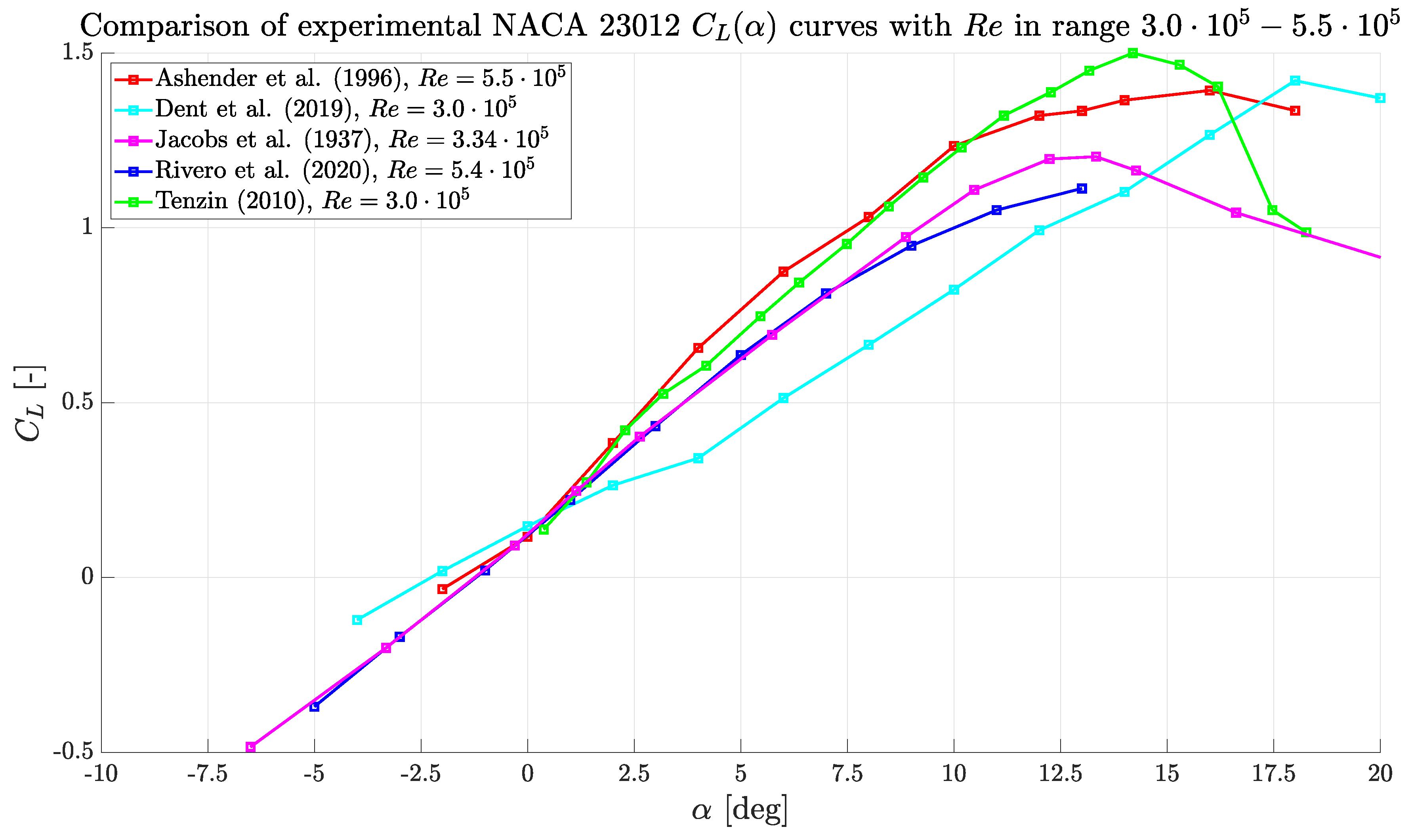
Figure 2.
C–type geometry, parameterized in R and L. The origin of the reference frame is located at the center of the semicircle.
Figure 2.
C–type geometry, parameterized in R and L. The origin of the reference frame is located at the center of the semicircle.
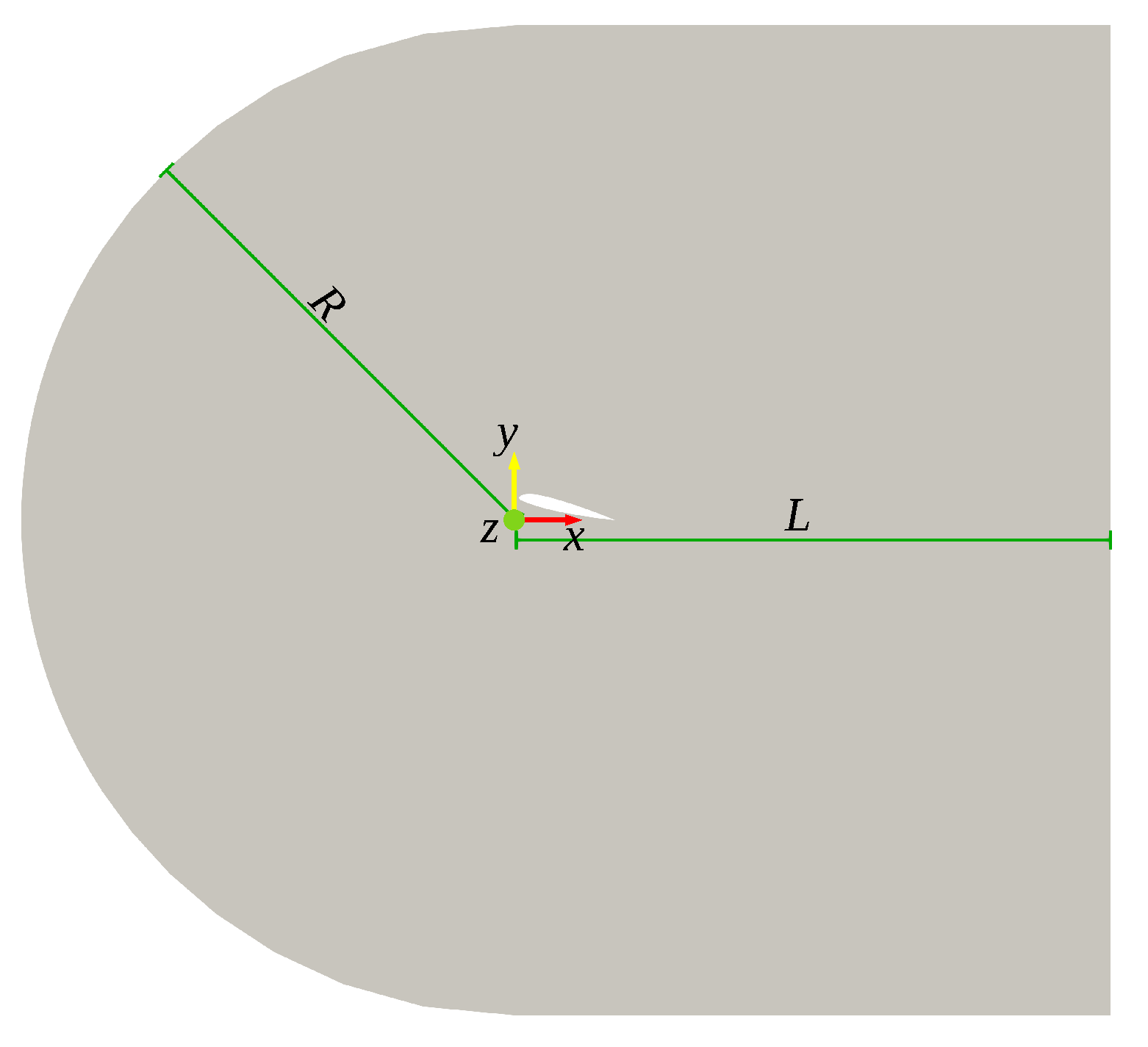
Figure 3.
Structured grid at .
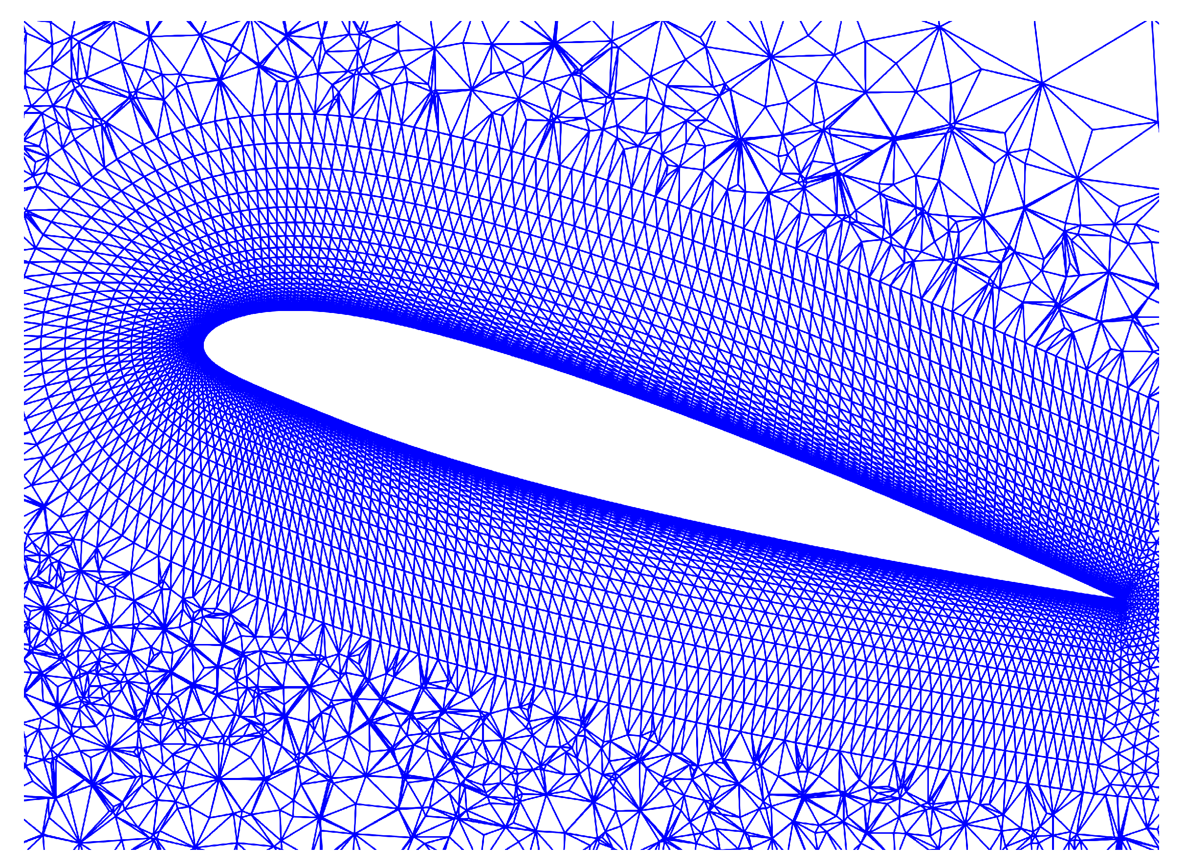
Figure 4.
coefficients of the preliminary tests. Note the peaks generated by the boundary conditions at for respectively. A similar behavior is experienced with data.
Figure 4.
coefficients of the preliminary tests. Note the peaks generated by the boundary conditions at for respectively. A similar behavior is experienced with data.
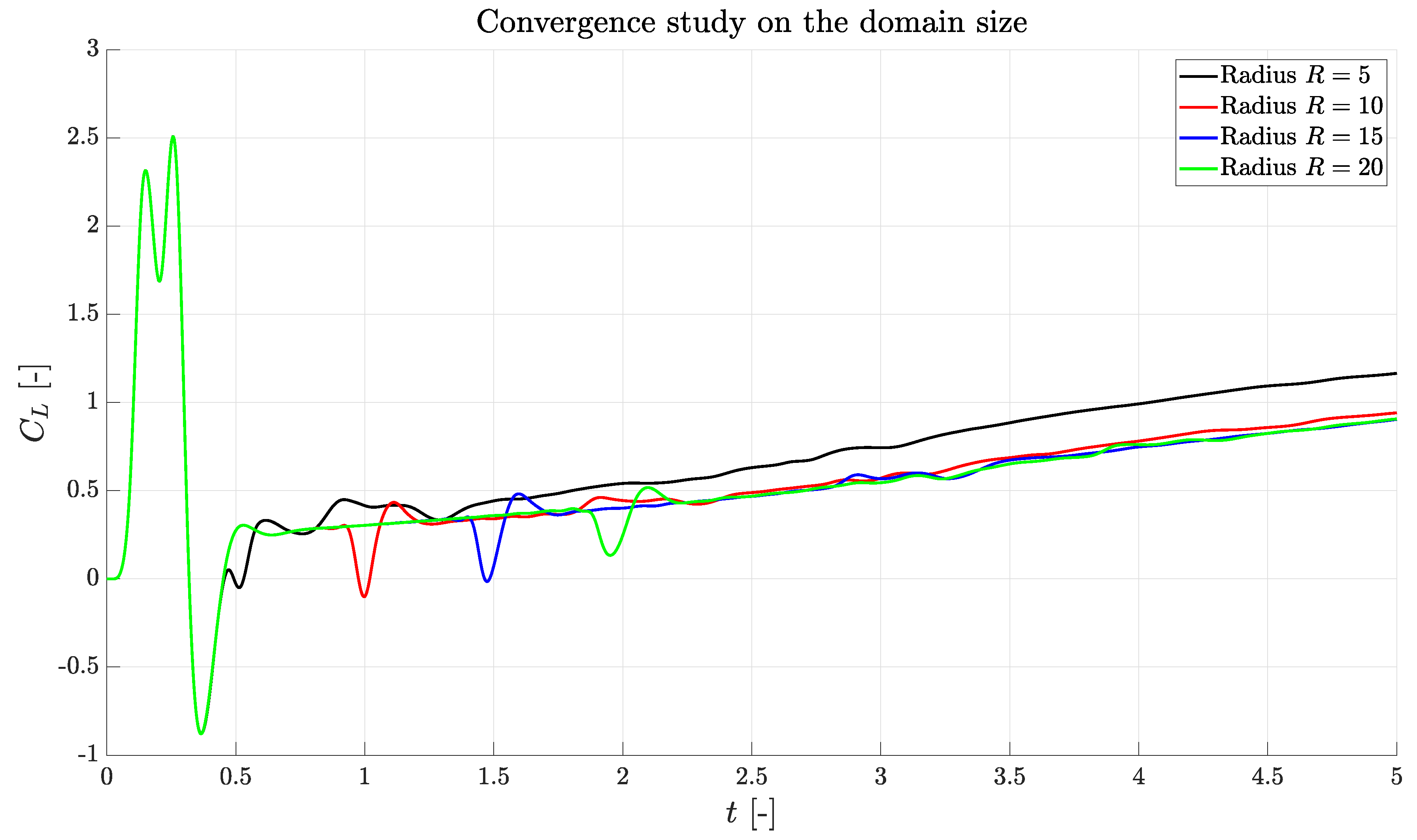
Figure 5.
Overall instantaneous velocity magnitude fields for .


Figure 6.
Zoom on the leading edge flow field at the different angles of attack, colored according to velocity magnitude. Note the presence of a progressively stronger laminar separation bubble.
Figure 6.
Zoom on the leading edge flow field at the different angles of attack, colored according to velocity magnitude. Note the presence of a progressively stronger laminar separation bubble.
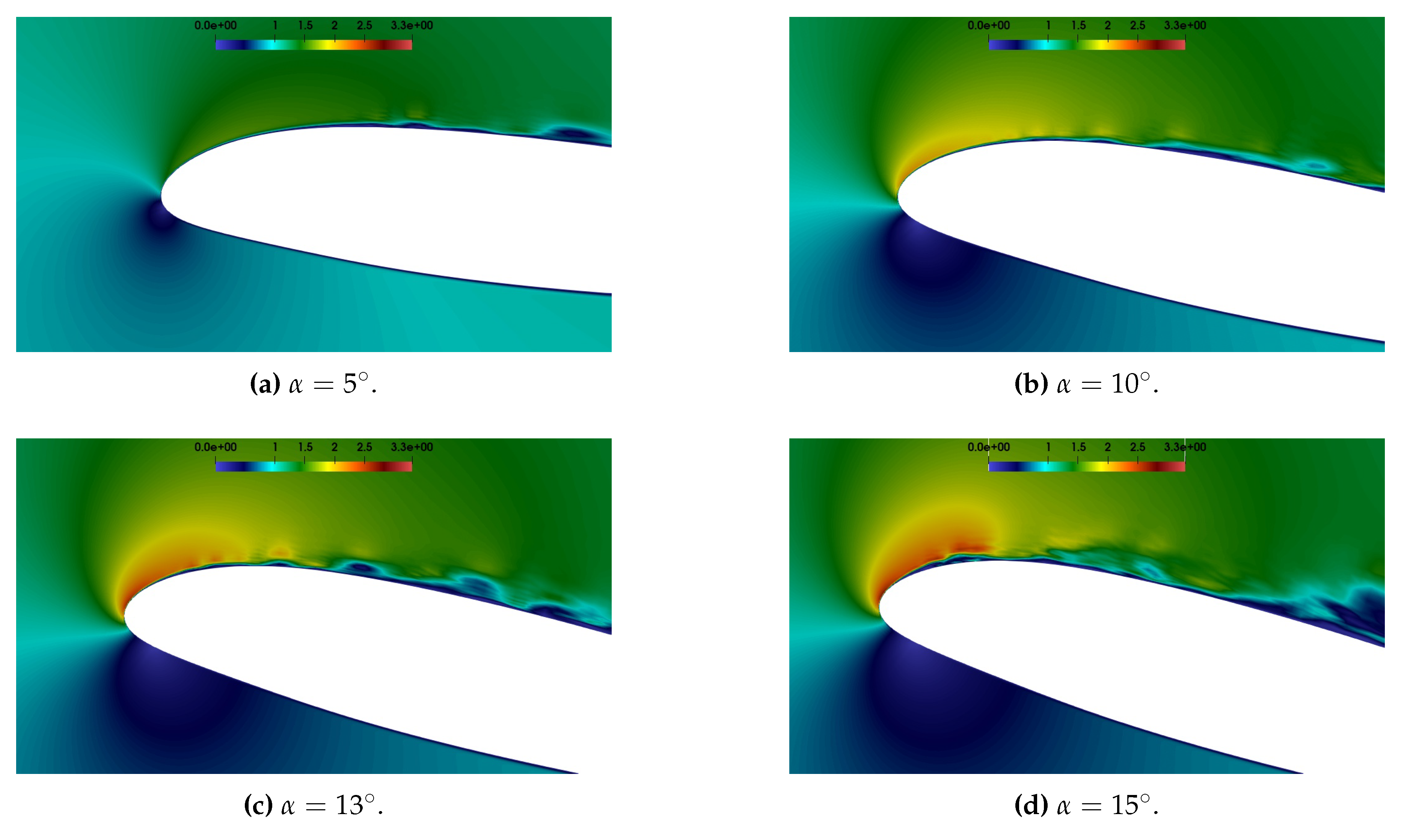
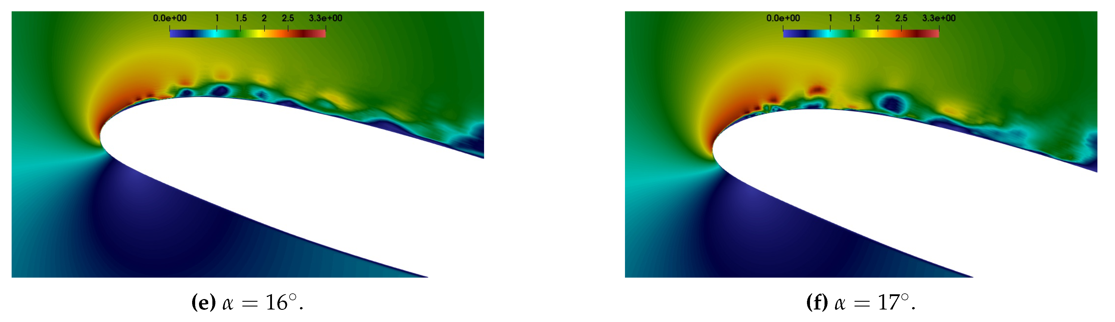
Figure 7.
Mean tangential velocity profiles according to .

Figure 8.
Graphic representation of the lines in Table 3 at .
Figure 8.
Graphic representation of the lines in Table 3 at .
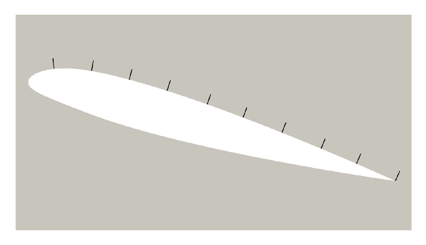
Figure 9.
Skin friction coefficient distribution according to . Only the higher angles of attack are reported, since they are the most meaningful ones.
Figure 9.
Skin friction coefficient distribution according to . Only the higher angles of attack are reported, since they are the most meaningful ones.
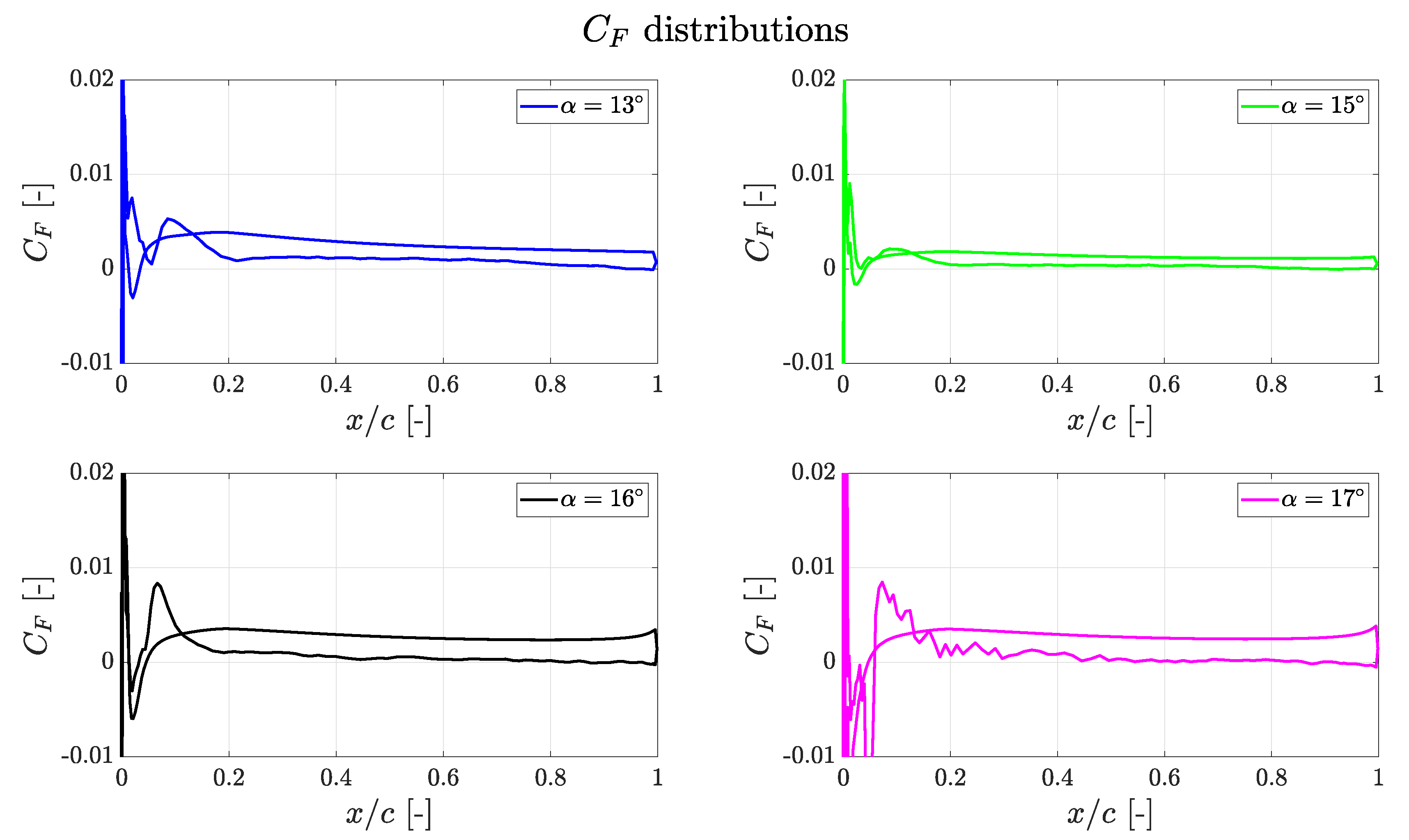
Figure 10.
Profiles at position 1, LSB location, 4, intermediate point, and 10, trailing edge for , and .
Figure 10.
Profiles at position 1, LSB location, 4, intermediate point, and 10, trailing edge for , and .
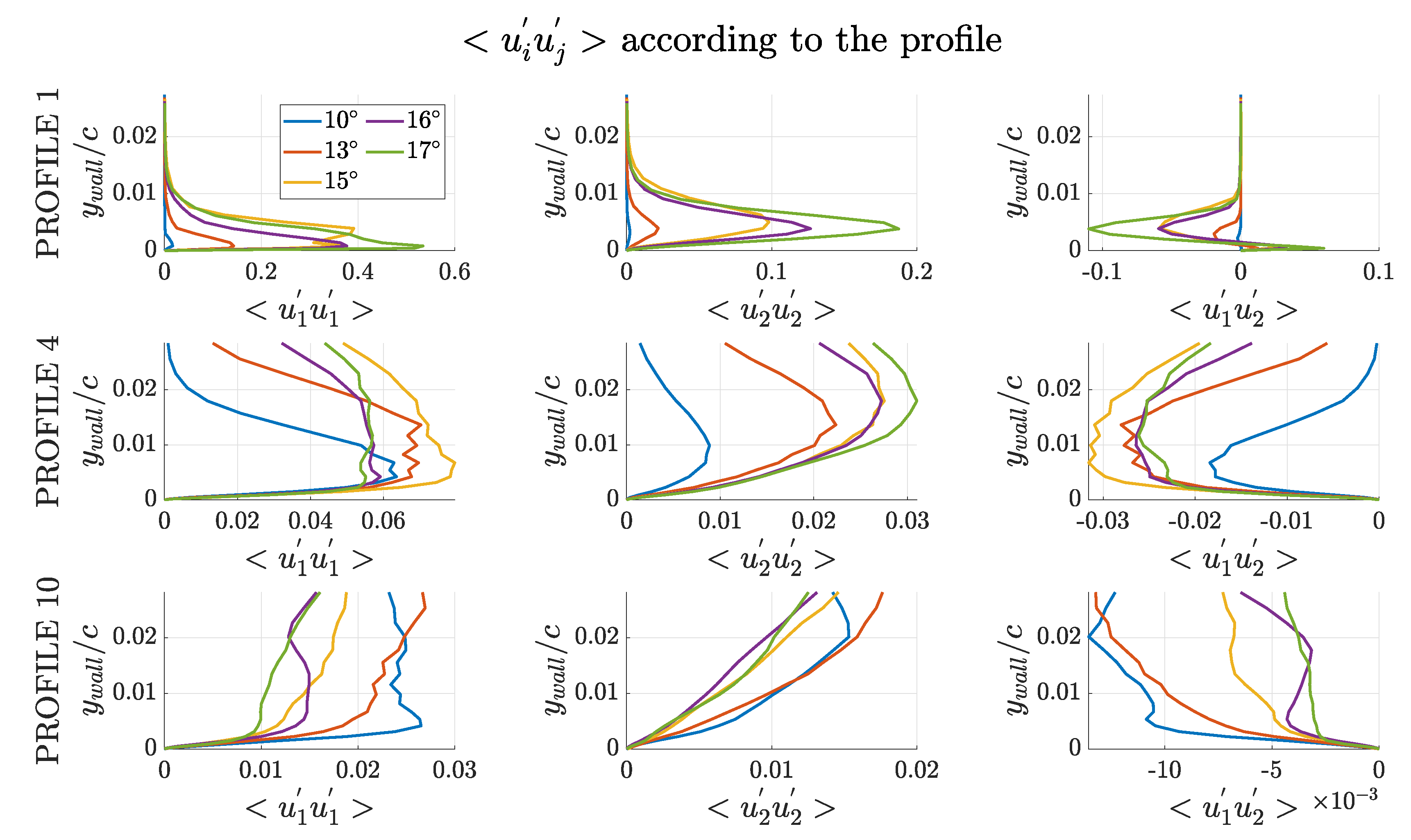
Figure 11.
LES force coefficients compared with experimental data [6,7,8,9,10]. Note that [7] does not provide information concerning .
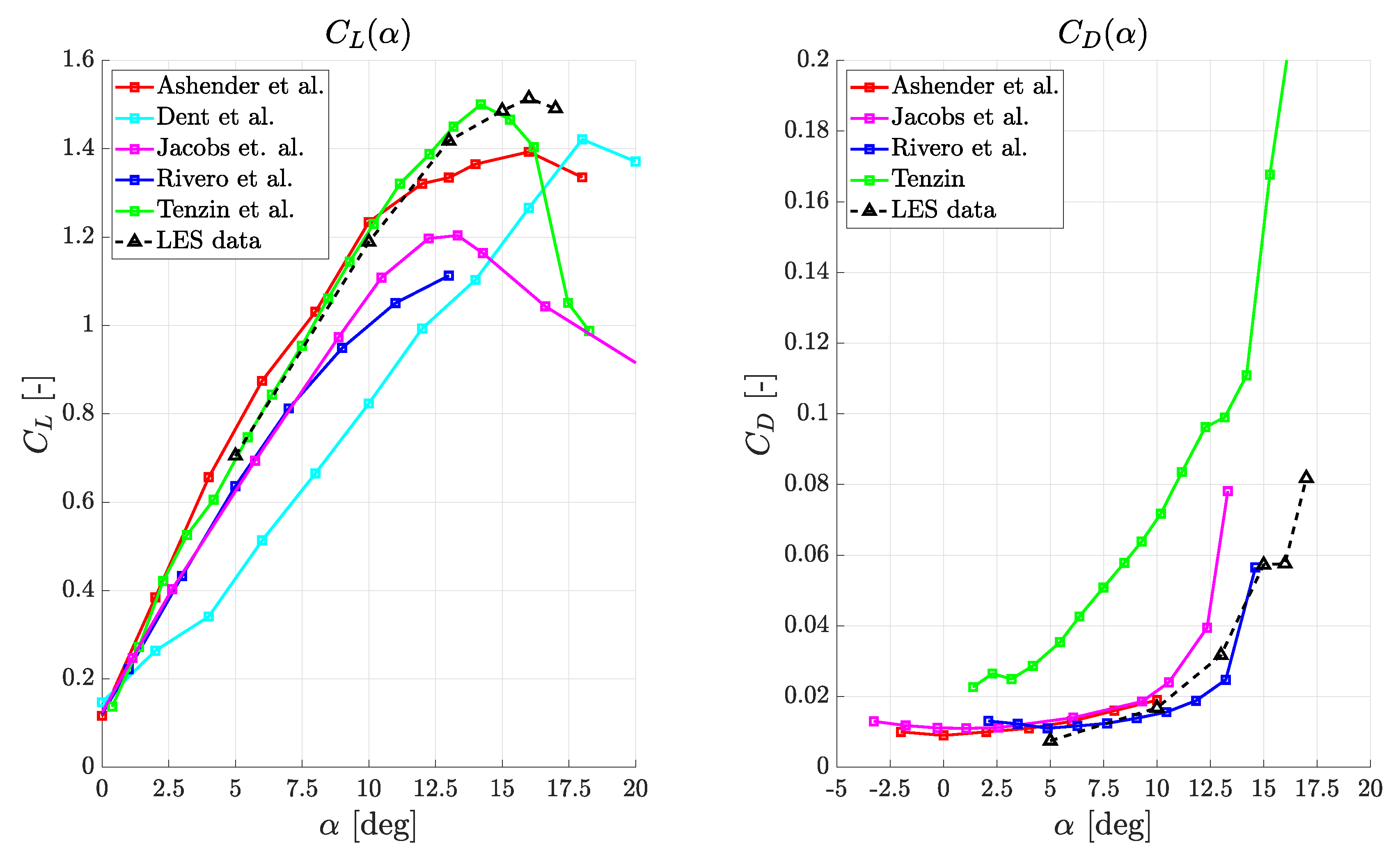

Table 1.
Domain size. All the values are intended dimensionless with respect to the chord length c.
| R | L | |
|---|---|---|
| 15 | 17 | 0.2 |
Table 2.
Average difference between the time histories at R and . Data are averaged for .
| R | ||
|---|---|---|
| 5 | 0.2336 | 0.0139 |
| 10 | 0.0333 | 0.0032 |
| 15 | 0.0043 | 0.0008 |
Table 3.
Chord position of the lines used for the velocity profiles.
| profile | [-] | profile | [-] |
|---|---|---|---|
| 1 | 0.102 | 6 | 0.600 |
| 2 | 0.201 | 7 | 0.702 |
| 3 | 0.300 | 8 | 0.805 |
| 4 | 0.400 | 9 | 0.898 |
| 5 | 0.505 | 10 | 1.000 |
Table 4.
Numerical force coefficients for NACA 23012.
| [deg] | [-] | [-] |
|---|---|---|
| 5 | 0.705 | 0.0075 |
| 10 | 1.189 | 0.0168 |
| 13 | 1.418 | 0.0317 |
| 15 | 1.486 | 0.0573 |
| 16 | 1.514 | 0.0576 |
| 17 | 1.491 | 0.0818 |
Disclaimer/Publisher’s Note: The statements, opinions and data contained in all publications are solely those of the individual author(s) and contributor(s) and not of MDPI and/or the editor(s). MDPI and/or the editor(s) disclaim responsibility for any injury to people or property resulting from any ideas, methods, instructions or products referred to in the content. |
© 2024 by the authors. Licensee MDPI, Basel, Switzerland. This article is an open access article distributed under the terms and conditions of the Creative Commons Attribution (CC BY) license (http://creativecommons.org/licenses/by/4.0/).
Copyright: This open access article is published under a Creative Commons CC BY 4.0 license, which permit the free download, distribution, and reuse, provided that the author and preprint are cited in any reuse.


