
Submitted:
30 May 2024
Posted:
30 May 2024
You are already at the latest version
Abstract
The examination of ampacity in overhead transmission lines offers a comprehensive overview, covering its definition, thermal evaluation methodologies, standards, practical applications, and the potential of high-temperature low-sag (HTLS) conductors. By navigating through static and dynamic approaches to thermal evaluation and detailing methodologies prescribed by international standards like those from CIGRE and IEEE, this study provides a solid understanding of how ampacity is determined and optimized. Furthermore, the exploration of HTLS conductors introduces a forward-looking perspective on enhancing transmission capacity whereas mitigating the need for extensive infrastructure modifications. Through an analysis of regional considerations and preferences using Slovak standards and CIGRE Technical Brochure 601, insights are provided on how environmental factors influence transmission line performance. The analysis of the transition from traditional ACSR to advanced ACCC (Aluminium Conductor Composite Core) conductors demonstrates the tangible benefits of adopting advanced conductor technologies in real-world scenarios.
Keywords:
ACCC
; ACSR
; ampacity
; CIGRE 601
; HTLS
; thermal rating
1. Introduction
The ampacity of overhead transmission lines is defined as the maximum electrical current that the lines can carry without reducing their electrical and mechanical properties. The most used conductors for overhead transmission lines are ACSR conductors, with aluminium forming the conductive layer. Manufacturers of these conductors state their maximum operating temperature in the range of 90 to 110°C. Prolonged exposure to temperatures beyond this range makes the material more brittle and reduces its lifespan. Overloading of electrical conductors appears as a recurring topic in many studies on various subjects, often either as a primary focus or as a limitation on transmission capacity due to issues with current overload [1,2,3].
Similarly, it is imperative to avoid exceeding its extension or maximum sag, which, if surpassed, would violate the minimum safe distances from the ground, objects,
2. Thermal Evaluation of Overhead Electrical Lines
The determination of ampacity is carried out through thermal evaluation, which is categorized into [5]:
- static ampacity (probabilistic approach, static line rating – SLR),
- dynamic ampacity (deterministic approach, dynamic line rating – DLR) with direct methods, and indirect methods.
The ampacity of long lines is often defined by stability limits or voltage constraints, whereas the ampacity of short lines is determined by temperature limitations [5].
2.1. Static Line Rating
In SLR, electrical grids are operated under the assumption that their conductors have a constant ampacity, which remains the same for every hour of the day, any day of the year, or any season. Entire regions with many overhead lines are considered areas with consistent meteorological conditions. Static assessment is a conservative estimate based on assumptions of weak convective cooling due to wind, high air temperatures, and solar radiation, where the calculation concerns theoretical rather than actual ampacity [6].
SLR is calculated using a thermal model based on the thermal balance of the bare conductor, low perpendicular wind speed (e.g., 0.5 m/s), seasonal air temperature close to the peak (e.g., 35°C or higher in summer), and full solar heating (e.g., 1000 W/m2), as described in CIGRE Technical Brochure 299 [7].
Meteorological conditions used for SLR evaluation vary depending on the region's environment and energy companies' risk tolerance. Each transmission line may have several types of SLR. These include normal rating (or continuous), long-term emergency rating, and short-term emergency rating [8].
2.2. Dynamic Line Rating
DLR dynamically adjusts ampacity in real-time in response to changing environmental conditions, aiming to maximize current loading at any given moment. The thermal ampacity of overhead lines can be influenced by both heating and cooling, resulting in fluctuations in performance either upward or downward. The thermal ampacity of the line increases when the conductor is cooled by the wind or when the ambient temperature decreases, allowing for greater power transmission through the line [4].
2.2.1. Indirect Dynamic Line Rating
DLR, with indirect methods, considers that the ampacity of transmission lines dynamically changes depending on environmental conditions. Ambient conditions encompass all climate-related factors, including ambient temperature, wind speed and direction, solar radiation intensity, and [1,4,5]. The evaluation of lines is indirectly calculated using meteorological data recorded or forecasted along the transmission line. This method is also known as weather-dependent line rating. Meteorological data, whether measured or predicted, are considered primary inputs into weather-dependent line rating systems. Weather sensors may be positioned along the transmission line to gather weather data for implementing DLR. Assessing the conductor's thermal balance equation forms the primary basis for weather-dependent line rating computations [5].
2.2.2. Direct Dynamic Line Rating
The direct method of DLR is based on directly measuring the properties of the electrical line, such as conductor temperature, mechanical stress on the line, and conductor sag. Line evaluation is typically calculated using additional data from a weather monitoring system. Whereas there are already numerous approaches discussed for estimating the DLR of overhead transmission lines [5].
2.2.3. Steady-State Dynamic Ampacity
When discussing DLR, it's important to specify two concepts related to the dynamic ampacity of overhead electrical conductors: steady-state dynamic ampacity (steady-state DLR) and transient dynamic ampacity (transient DLR).
The current size at which the conductor temperature stabilizes at a certain value is referred to as the steady-state dynamic ampacity. In this calculation, it is assumed that all operating parameters are constant (do not change over time), meaning the conductor is in thermal equilibrium. Therefore, this calculation is associated with the stable temperature of the conductor before or after the initiation or termination of a transient event caused by the change in one operating parameter or the change in multiple operating parameters simultaneously. Steady-state solution often focuses on the opposite question, i.e., determining the stable conductor temperature with a known current flowing through the conductor and constant climatic conditions [9].
2.2.4. Transient Dynamic Ampacity
If a conductor has a defined thermal ampacity, it can be used for short-term current overload to ensure that the maximum allowed conductor temperature is not exceeded. This short-term current overload is known as transient dynamic ampacity and is associated with a limited duration of overload. This computational approach focuses on the change in conductor temperature over time, considering changes in specific operating factors (climatic conditions and current flowing through the conductor) [9].
3. Thermal Balances of Overhead Electrical Lines Designed According to Standards
The International Council on Large Electric Systems (CIGRE) and IEEE address standards that explain algorithms for estimating ampacity and conductor temperature. Both techniques (CIGRE and IEEE) are based on the thermal balance of heat gained and lost in the conductor, according to the load and environmental factors [10].
The first CIGRE method calculates the conductor temperature using steady-state conditions, whereas the second method estimates its temperature using dynamic equilibrium, which considers the thermal inertia of the conductor. In steady-state conditions, the basic thermal balance is defined as [10]:
where:
- Pc represents cooling due to convection (W/m),
- Pr represents cooling due to radiation to the surroundings (W/m),
- PS represents heating due to solar radiation (W/m),
- Pj represents heating due to Joule effect (W/m),
- Pm represents heating due to magnetic effect (W/m).
If the thermal inertia of the conductor is considered, the following dynamic thermal balance is applied instead of equation [10]:
where:
- m is the mass per unit length of the conductor (kg/m),
- c is the specific heat capacity of the conductor (J/(kg·K)),
- Tc is the conductor temperature of the conductor (°C).
The equation for the steady-state thermal balance in IEEE Standard 738 is represented by [11]:
where [11]:
- Pr represents cooling due to radiation to the surroundings (W/m),
- Pc represents cooling due to convection (W/m),
- PS represents heating due to solar radiation (W/m),
- PJ represents heating due to the Joule effect (W/m).
Differences in methodologies according to standards [11]:
- both methods consider meteorological factors such as wind speed and direction, ambient temperature, and solar radiation, but they calculate the thermal balance differently,
- solar heating (solar radiation) is calculated by considering the position of the sun in different seasons. CIGRE employs a more complex algorithm that considers direct, diffuse, and reflected radiation,
- CIGRE approaches convective cooling using Morgan correlations based on the Nusselt number, whereas IEEE utilizes McAdams correlations based on the Reynolds number.
4. Considerations Relating to the Use of High Temperature Low Sag Conductors
The current trend reflects a continual escalation in energy consumption, accompanied by challenges such as unplanned large-scale transfers of electrical energy from one region of the power system to another. This often arises due to fluctuations in the production of renewable energy sources concentrated in specific locales. Consequently, there arises a critical need to augment the transmission capacity of overhead electrical lines. As mentioned previously, one viable approach to address this issue is the replacement of conductors. A promising solution lies in the adoption of HTLS conductors in lieu of traditional ACSR conductors, which operate within a temperature range of 80 °C to 100 °C [9,12].
To minimize the necessity for structural modifications to transmission lines, HTLS conductors must operate at significantly higher temperatures than conventional conductors, whereas ensuring compliance with permissible sag limits and without inducing substantial increases in original mechanical tension, ice loading, or wind loading. HTLS conductors are engineered for applications necessitating continuous operation at conductor temperatures exceeding 100 °C, designed to withstand emergency conditions at temperatures exceeding 150 °C. The appealing characteristics of high-temperature conductors come with elevated costs. However, these higher costs are deemed acceptable if they facilitate cost reduction or prevention of expenses associated with structural alterations to transmission lines [9].
Current commercially available types of HTLS conductors, as well as the materials employed in the construction of their cores and casings, are succinctly described in technical manuals such as CIGRE 425, CIGRE 331, and CIGRE 244 (Table 1). Additionally, CIGRE Technical Brochure 331 addresses the impact of HTLS conductors on insulators, providing comprehensive insights into their application and integration within existing power infrastructure [9].
5. Ampacity of Overhead Transmission Lines in Slovakia Applying CIGRE Technical Brochure 601
In practical scenarios, following the guidelines outlined in Slovak standards STN EN 50341-2-23, the conductor's maximum permissible current value at its highest design temperature is utilized within the designated parameters:
- ambient temperature Ta of +35 °C,
- wind speed V of 0.5 m/s at an angle θ of 45 ° to the axis of the conductor,
- global solar radiation intensity IT of 1000 W/m2,
- absorption coefficient αs of 0.5,
- emissivity coefficient εs of 0.5.
One of the most prevalent types of conductors employed in overhead transmission lines are ACSR conductors, which can be installed individually or bundled together depending on the voltage rating. Table 2 presents the essential technical characteristics of selected ACSR conductors necessary for analysing and computing the maximum allowable current value based on varying climatic conditions. In this analysis, we also consider a maximum permissible conductor temperature Ts of 80 °C and an altitude y of 208 meters.
The static ampacity of the described conductors encompasses the conditions outlined in the referenced standards. As previously stated, this value remains constant throughout the entire period or year. To simplify matters, the static ampacity is presented for a 24-hour interval, as depicted in Figure 3.
Figure 4 illustrates the relationship between the maximum permissible current value across various types of ACSR conductors and the ambient temperature. As the conductor diameter increases, its ampacity experiences proportional growth. Conversely, as the ambient temperature rises, the ampacity diminishes. When comparing SLR and DLR, it can be stated that with a change in ambient temperature whereas maintaining other conditions according to the STN standards, DLR is advantageous in 93% of cases.
The graph depicted in Figure 5 illustrates the correlation between the maximum allowable current value for various types of ACSR conductors and the wind speed, whereas adhering to the meteorological parameters specified in the STN for SLR. In this graphical relationship, SLR is advantageous in only 5% of cases. Similarly, as the conductor diameter increases, the ampacity experiences a positive increment.
The graphical visualization in Figure 6 demonstrates the correlation between the maximum allowable current value of different ACSR conductor types and the wind direction, whereas maintaining other static weather conditions according to the SLR norm. The conductor diameter positively influences the ampacity. Given that the STN specifies a 45-degree angle, DLR is more optimal in 50% of cases.
The final meteorological parameter regulated is the relationship between the maximum permissible current value of various ACSR conductor types and the intensity of solar radiation (Figure 7). The global intensity of solar radiation is inversely proportional to the ampacity. From the values used for the graphical dependency, it can be stated that DLR is advantageous 99% of the time.
6. Application of HTLS Conductors to Increase the Ampacity of Transmission Overhead Lines
This section focuses on increasing the permissible load current achievable by replacing ACSR conductors with ACCC conductors. However, there are numerous possibilities to increase transmission capacities [13]:
- constructing new power lines,
- upgrading existing power lines to higher voltages,
- increasing the permissible load current,
- structural modifications to overhead power lines,
- installing compensating devices,
- constructing new substations.
The conductor selection was based on achieving a similar diameter and weight compared to the ACSR conductors. The selection process involved comparing the diameter and weight of the conductors. The conductor diameter influences the wind and icing loads. As the diameter increases, there is a larger windage area or more ice accumulates on the conductor. With greater conductor weight, the loads on pylon structures increase. When selecting an equivalent conductor, it is necessary for these parameters to closely resemble those of the original conductors. The conductor parameters are provided in the following Table 3.
Following the renewed utilization of standard STN EN 50341-2-23 for ACCC conductors, the SLR is illustrated in Figure 8. Figure 9, Figure 10, Figure 11 and Figure 12 illustrate the change in meteorological conditions, whereas other factors are maintained statically according to STN for SLR compared to alternative ACSR conductors. Just as with ACSR conductors, graphs for ACCC conductors confirm the electrical, thermal, and mechanical dependencies of this issue. A significant change is the pronounced increase in ampacity.
For a clear and concise comparison between ACCC and ACSR conductors, a graphical representation depicting the temperature dependency on current loading was provided in Figure 13. Meteorological conditions were set according to STN standards for SLR. The maximum conductor temperature for ACSR conductors is 80 °C, whereas for ACCC, it is 200 °C. A comparison of values is described in Table 4.
The dynamic steady-state ampacity was applied to the transmission line V427 Rimavská Sobota – Moldava. This line utilizes the conductor 352-AL1/59-ST1A, and weather data were obtained on November 25, 2021. Current load data were obtained from PMU units in the electric power system of the Slovak Republic, and weather data were obtained from the distribution system. Figure 14 illustrates the resulting steady-state dynamic ampacity with the original ACSR conductor for a 24-hour interval, with the graph also depicting surrounding meteorological conditions.
Figure 15 displays the replacement of the ACSR conductor with its compatible ACCC conductor (LUBBOCK). The ampacity increased by at least 694.26 A and at most 973.29 A with the replacement of the ACCC conductor, resulting in an average increase of 778.22 A. The ACCC conductor LUBBOCK operates at a temperature of 200 °C, which is its maximum allowable operating temperature.
7. Discussion
Maintaining the ampacity of overhead transmission lines requires careful consideration of factors like conductor temperature, mechanical integrity, and adherence to safety standards. Overloading and exceeding maximum sag pose risks to both performance and safety, emphasizing the need for strict adherence to design limits and operational guidelines to ensure reliable power transmission.
CIGRE and IEEE establish standards for estimating ampacity and conductor temperature, both based on heat balance equations considering heat gained and lost in the conductor, influenced by loading and environmental factors. Determining ampacity involves thermal assessment, divided into static and dynamic approaches. Static assessment assumes constant ampacity under various conditions, whereas dynamic methods adjust ampacity in real-time based on changing environmental factors. These approaches are crucial for ensuring safe and efficient operation of overhead transmission lines.
The adoption of HTLS conductors presents a promising solution to meet the escalating energy consumption challenges, particularly in addressing unplanned large-scale energy transfers caused by renewable energy fluctuations. These conductors, engineered for operation at elevated temperatures exceeding 100 °C and emergency conditions exceeding 150 °C, offer enhanced transmission capacity without necessitating significant structural modifications to existing lines, despite their higher costs.
The application of Slovak standards and CIGRE Technical Brochure 601 provides insights into the ampacity of overhead transmission lines in Slovakia, considering factors like ambient temperature, wind speed, and solar radiation intensity. Analysis reveals preferences for certain conductor types under specific conditions, with DLR often proving advantageous due to its performance across various meteorological parameters.
The analysis outlines strategies for enhancing permissible load current by transitioning from ACSR to ACCC conductors. The selection process prioritizes maintaining similar conductor diameter and weight to mitigate impacts on wind and icing loads, ensuring compatibility with existing infrastructure. Utilizing standard STN EN 50341-2-23 for ACCC conductors reveals substantial increases in ampacity compared to traditional ACSR conductors, highlighting the considerable advantages of adopting advanced conductor technologies.
Utilizing dynamic steady-state ampacity analysis on the transmission line V427 Rimavská Sobota – Moldava, replacing the ACSR conductor with a compatible ACCC conductor (LUBBOCK) significantly increased ampacity. With an average increase of 778.22 A, ranging from 694.26 A to 973.29 A, this highlights the efficacy of adopting advanced conductor technologies for enhancing transmission line performance.
Author Contributions
Conceptualization, F.M., L.B. W.M. and P.P; methodology, F.M., L.B. and P.P.; software, F.M., L.B. and W.M.; validation, F.M. and L.B.; formal analysis, W.M. and P.P.; investigation, W.M. and P.P.; resources, F.M., L.B. and W.M.; data curation, F.M., and P.P.; writing—original draft preparation, F.M. and L.B.; writing—review and editing, F.M. and P.P..; visualization, F.M. and W.M.; supervision, F.M. and L.B.; project administration, L.B.; funding acquisition, L.B. All authors have read and agreed to the published version of the manuscript.
Funding
Slovak Research and Development Agency under contracts No. APVV-19-0576 and APVV-21-0312.
Institutional Review Board Statement
Not applicable.
Informed Consent Statement
Not applicable.
Data Availability Statement
Not applicable.
Acknowledgments
This work was supported by the Slovak Research and Development Agency under contracts No. APVV-19-0576 and APVV-21-0312.
Conflicts of Interest
The authors declare no conflict of interest.
References
- Bena, L.; Kolcun, M.; Medved, D.; Pavlik, M.; Conka, Z.; Kiraly, J. The Influence of Climatic Conditions on the Dynamic Ampacity of External Lines. Elektroenergetika 2022, 15(2), 1–4. [Google Scholar]
- Kladar, D. Dynamic Line Rating in the World - Overview. 2014, 1–8.
- Pijarski, P.; Kacejko, P. Elimination of Line Overloads in a Power System Saturated with Renewable Energy Sources. Energies 2023, 16(9), 3751–3751. [Google Scholar] [CrossRef]
- International Renewable Energy Agency IRENA. Innovation Landscape Brief: Electric-Vehicle Smart Charging; International Renewable Energy Agency (IRENA), 2019.
- Karimi, S.; Musilek, P.; Knight, A. M. Dynamic Thermal Rating of Transmission Lines: A Review. Renewable and Sustainable Energy Reviews 2018, 91, 600–612. [Google Scholar] [CrossRef]
- Simms, M.; Meegahapola, L. Comparative Analysis of Dynamic Line Rating Models and Feasibility to Minimise Energy Losses in Wind Rich Power Networks. Energy Conversion and Management 2013, 75, 11–20. [Google Scholar] [CrossRef]
- Alberdi, R.; Fernandez, E.; Albizu, I.; Bedialauneta, M. T.; Fernandez, R. Overhead Line Ampacity Forecasting and a Methodology for Assessing Risk and Line Capacity Utilization. International Journal of Electrical Power & Energy Systems 2021, 133, 107305. [CrossRef]
- Douglass, D.; Gentle, J.; Nguyen, H.-M.; Chisholm, W.; Xu, C.; Goodwin, T.; Chen, H.; Nuthalapati, S.; Hurst, N.; Grant, I.; Jardini, J. A.; Kluge, R.; Traynor, P.; Davis, C. A Review of Dynamic Thermal Line Rating Methods with Forecasting. IEEE Transactions on Power Delivery 2019, 34(6), 2100–2109. [Google Scholar] [CrossRef]
- Margitova, A. Increasing the Transmission Capacity of External Power Lines by Calculating the Dynamic Ampacity. PhD Thesis, TUKE, 2021, pp. 11–105.
- Arroyo, A.; Castro, P.; Martinez, R.; Manana, M.; Madrazo, A.; Lecuna, R.; Gonzalez, A. Comparison between IEEE and CIGRE Thermal Behaviour Standards and Measured Temperature on a 132-KV Overhead Power Line. Energies 2015, 8(12), 13660–13671. [Google Scholar] [CrossRef]
- Karunarathne, E.; Wijethunge, A.; Ekanayake, J. Enhancing PV Hosting Capacity Using Voltage Control and Employing Dynamic Line Rating. Energies 2021, 15(1), 134. [Google Scholar] [CrossRef]
- Beryozkina, Svetlana; Sauhats, Antans; Banga, A.; Jakusevics, I. Evaluation of Thermal Rating Methods Based on the Transmission Line Model. Latvian Journal of Physics and Technical Sciences 2013, 50 (09), pp 1–6. [CrossRef]
Figure 1.
Factors affecting the ampacity of a conductor.
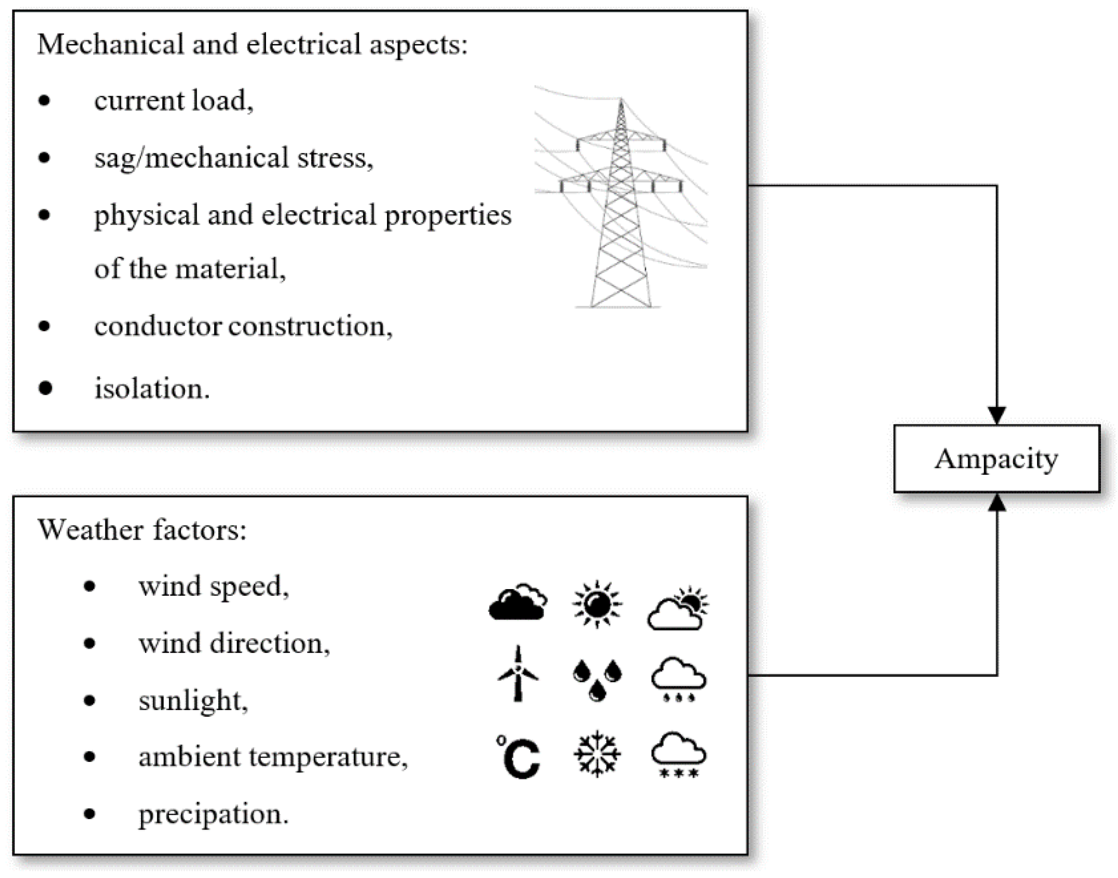
Figure 2.
Thermal balance of an overhead conductor according to IEEE 738.
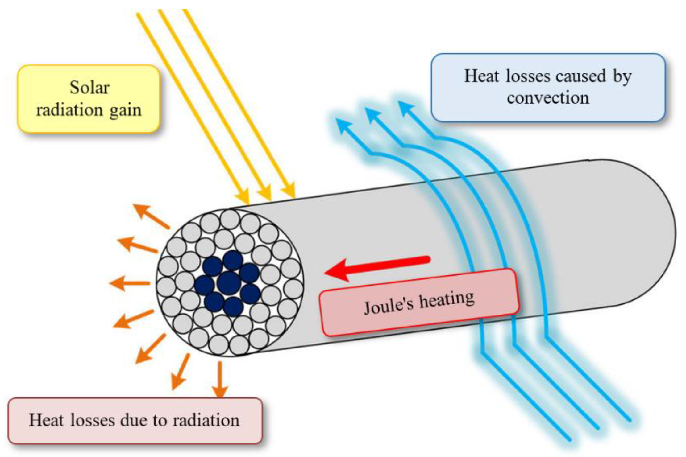
Figure 3.
Static ampacity Imax for the utilized ACSR conductors.
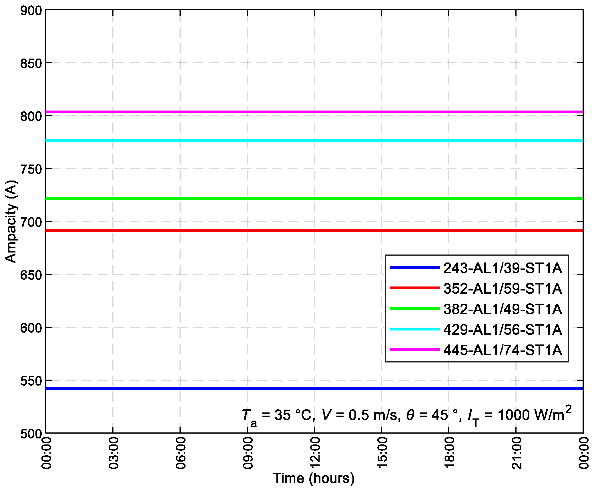
Figure 4.
The relationship between the maximum permissible current value Imax for different types of ACSR conductors and the ambient temperature Ta.
Figure 4.
The relationship between the maximum permissible current value Imax for different types of ACSR conductors and the ambient temperature Ta.
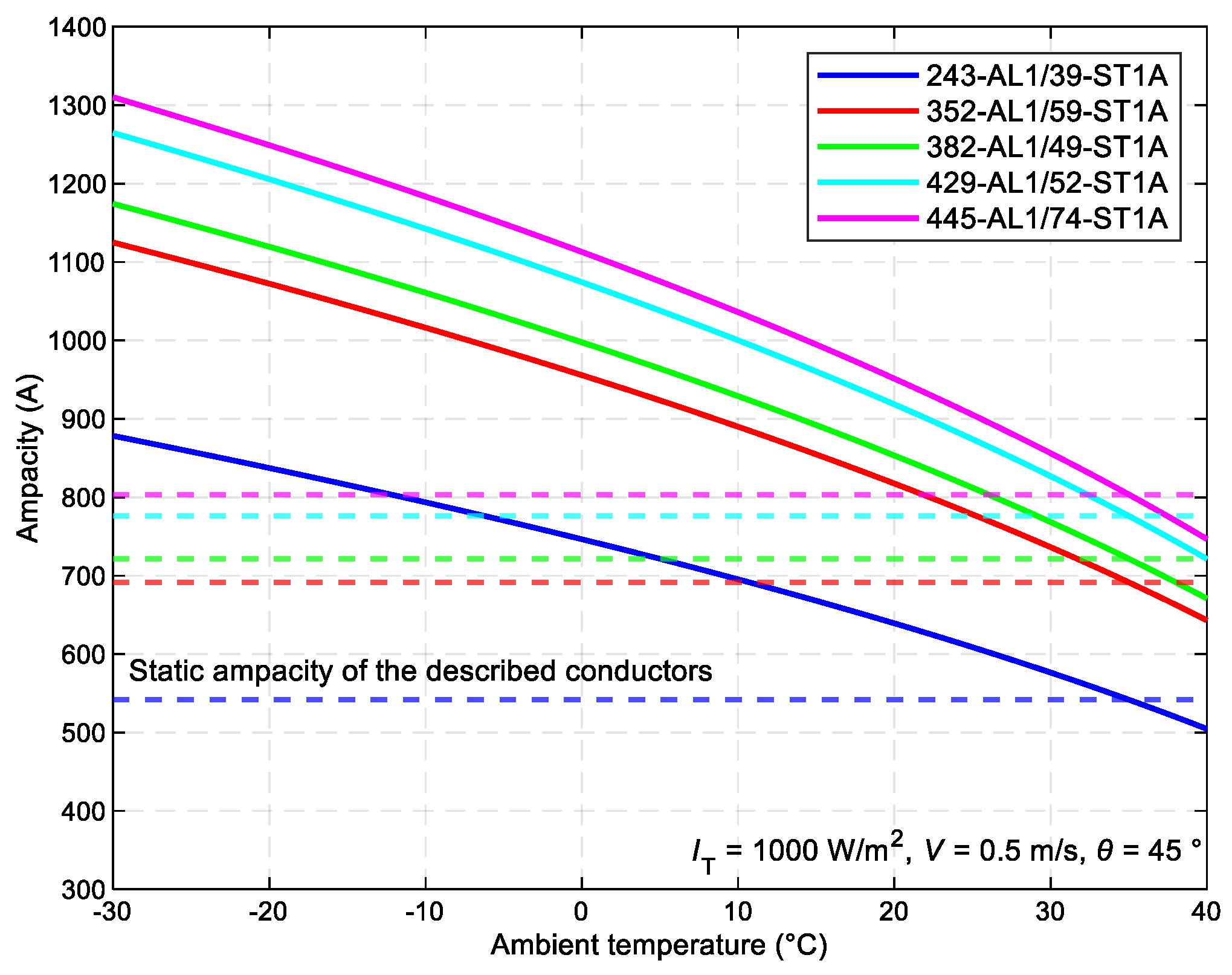
Figure 5.
The relationship between the maximum allowable current value Imax of different ACSR conductor types and the wind speed V.
Figure 5.
The relationship between the maximum allowable current value Imax of different ACSR conductor types and the wind speed V.
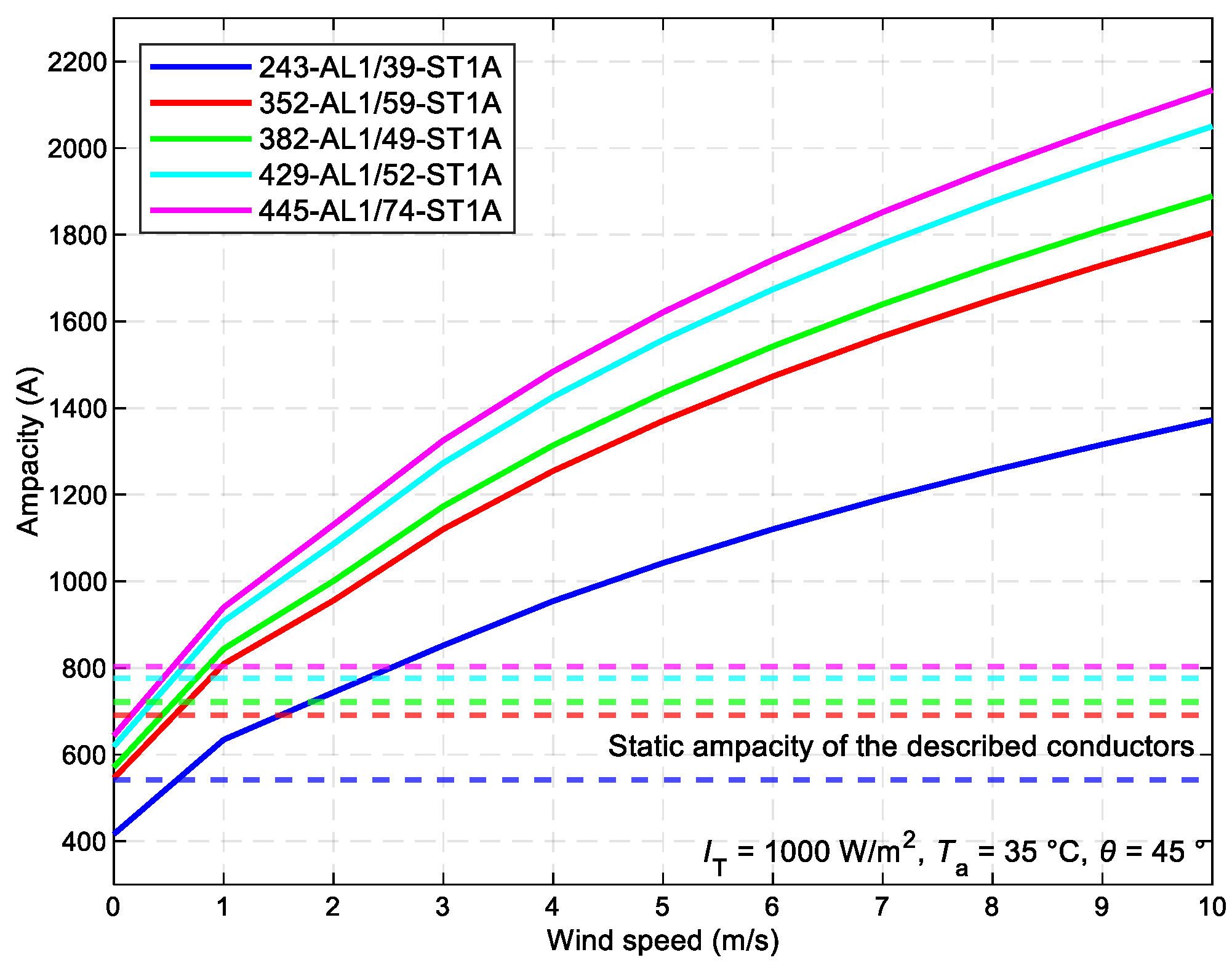
Figure 6.
The correlation between the maximum allowable current value Imax of diverse ACSRconductor types and the wind direction θ.
Figure 6.
The correlation between the maximum allowable current value Imax of diverse ACSRconductor types and the wind direction θ.
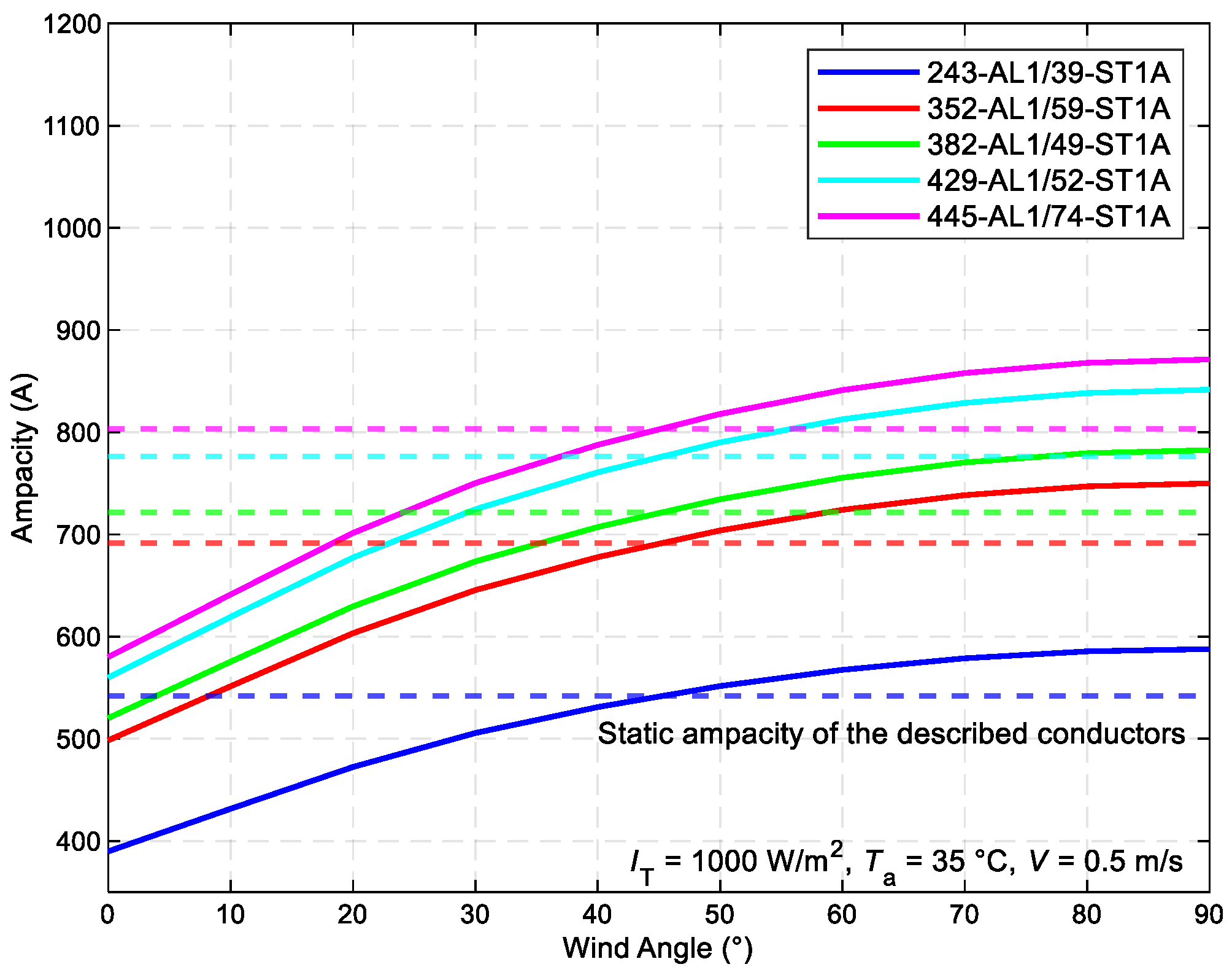
Figure 7.
The relationship between the maximum permissible current value Imax of various ACSR conductor types and the intensity of solar radiation IT.
Figure 7.
The relationship between the maximum permissible current value Imax of various ACSR conductor types and the intensity of solar radiation IT.
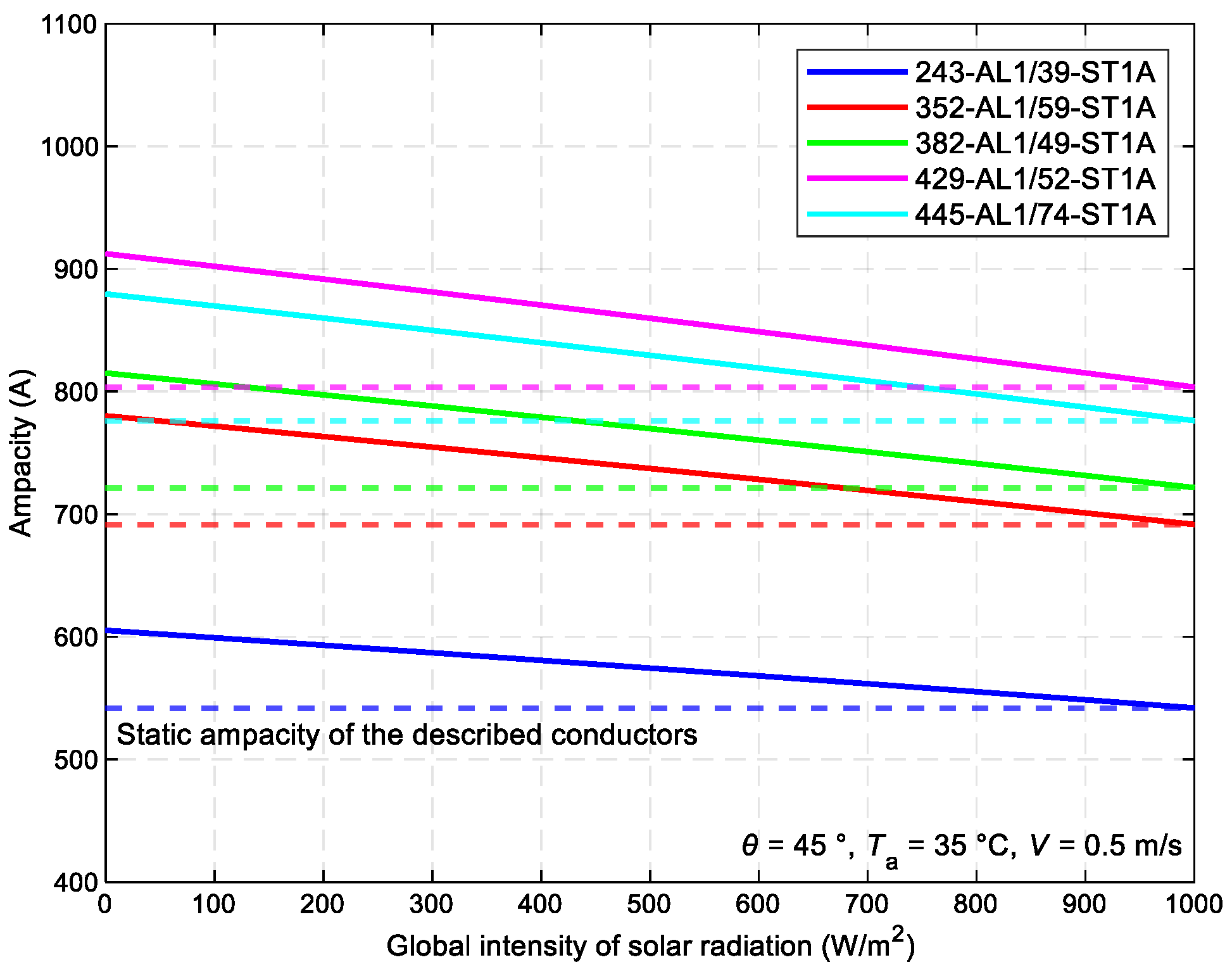
Figure 8.
Static ampacity Imax for the employed ACCC conductors.
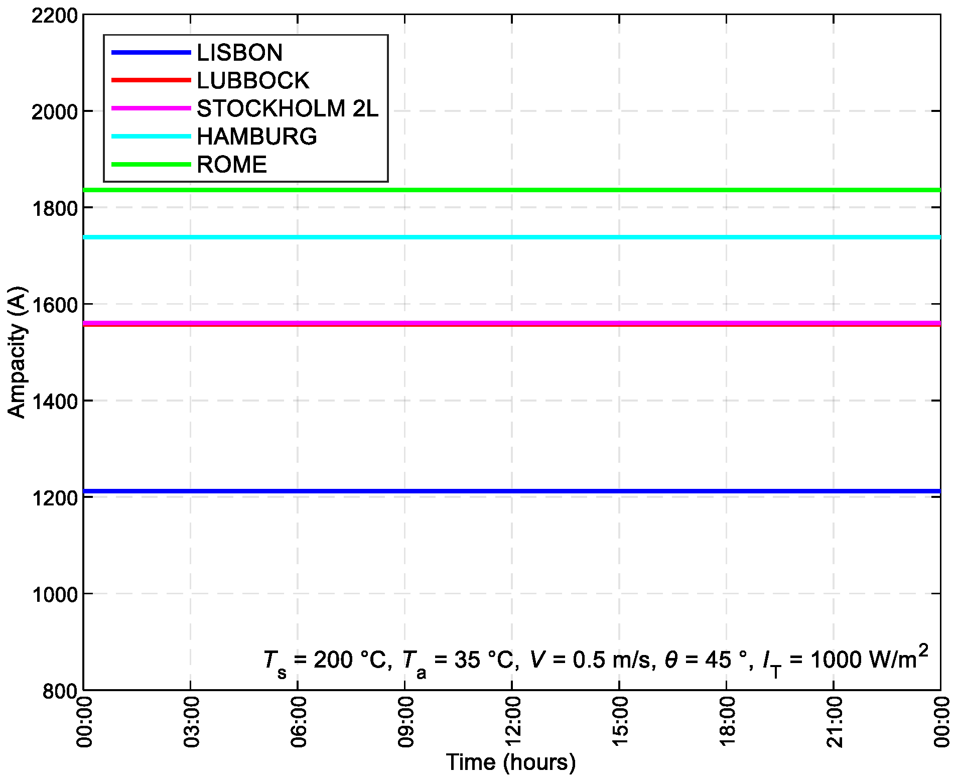
Figure 9.
The correlation between the maximum allowable current value Imax for various types of ACCC conductors and ambient temperature Ta.
Figure 9.
The correlation between the maximum allowable current value Imax for various types of ACCC conductors and ambient temperature Ta.
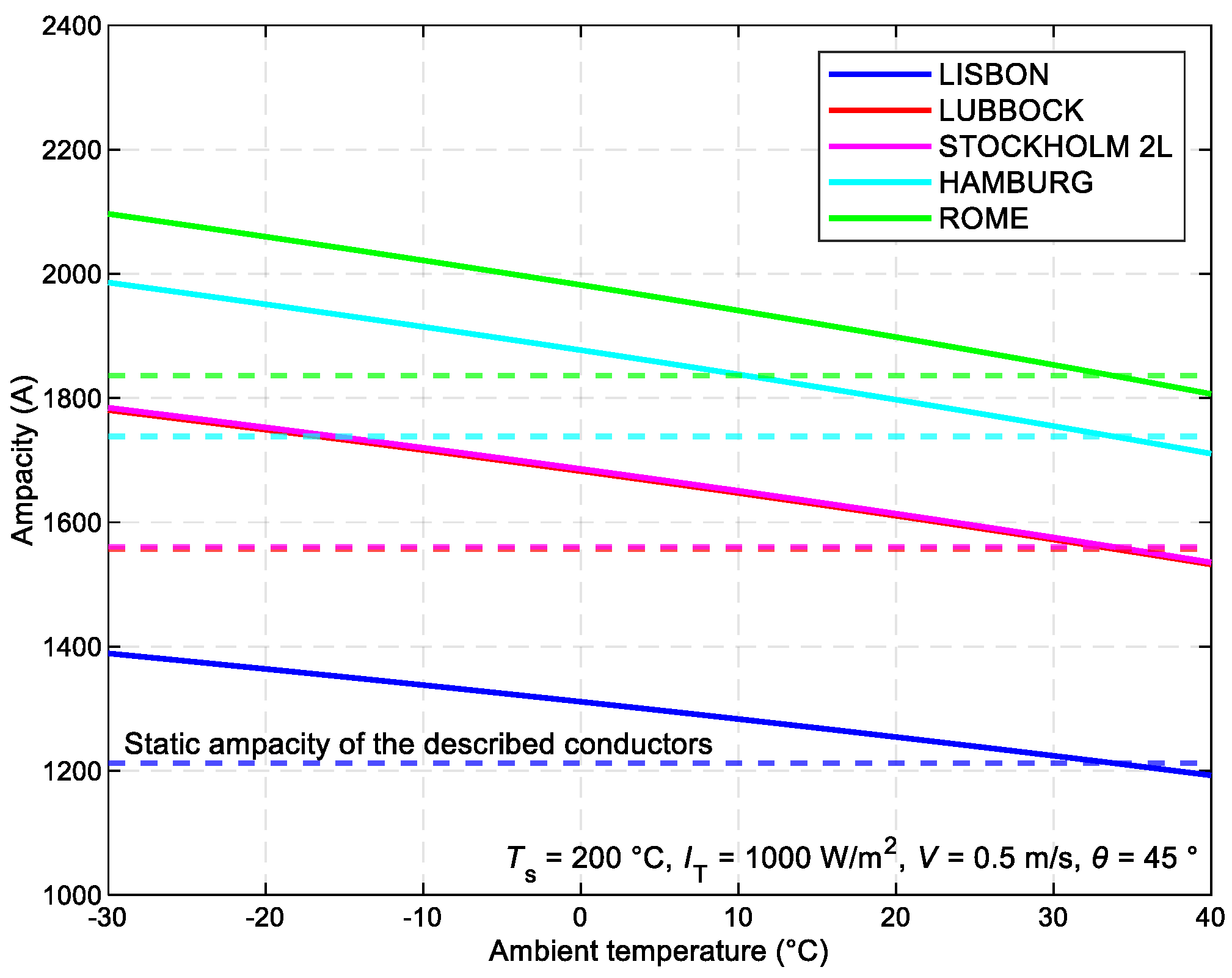
Figure 10.
The correlation between the maximum allowable current value Imax of various ACCC conductor types and the wind speed V.
Figure 10.
The correlation between the maximum allowable current value Imax of various ACCC conductor types and the wind speed V.
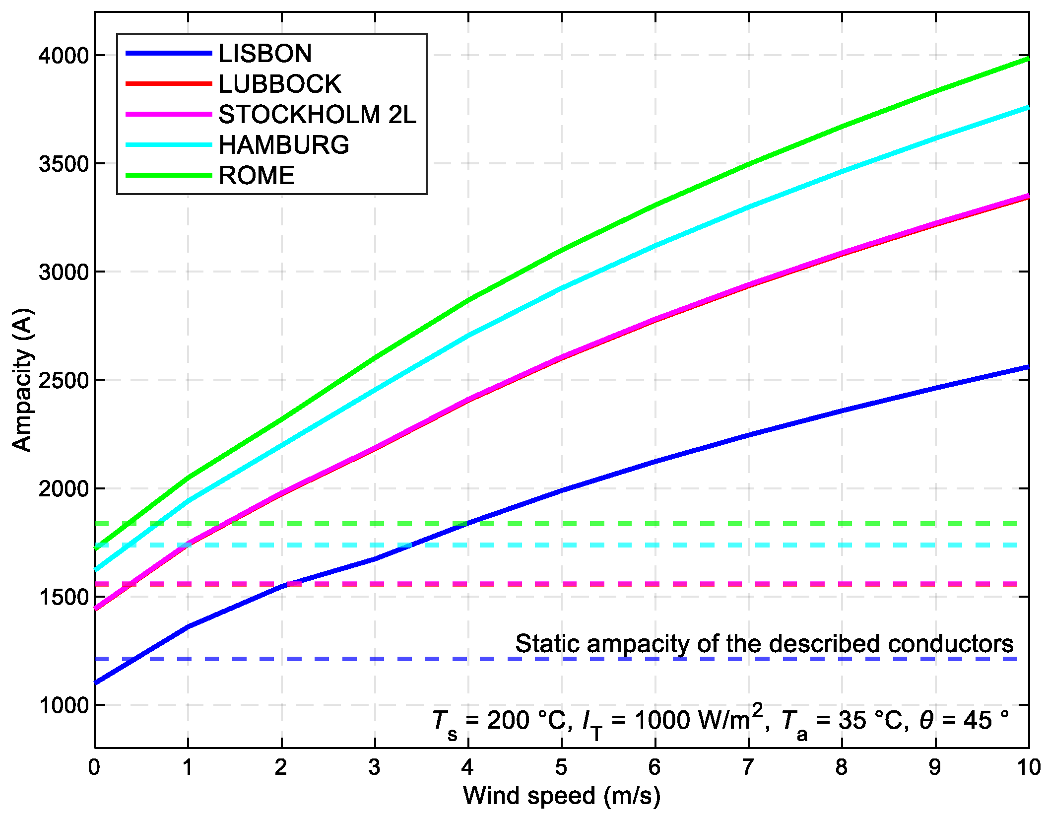
Figure 11.
The relationship between the maximum allowable current value Imax of different ACCC conductor types and the wind direction θ.
Figure 11.
The relationship between the maximum allowable current value Imax of different ACCC conductor types and the wind direction θ.
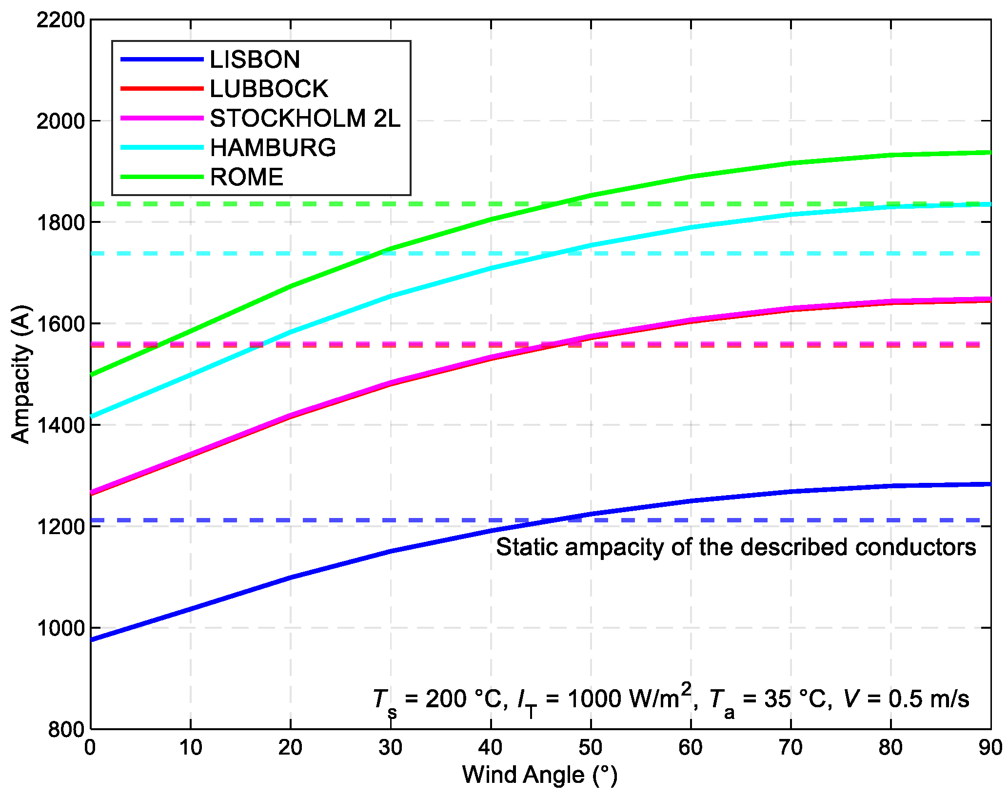
Figure 12.
The correlation between the maximum allowable current value Imax of different types of ACCC conductors and the intensity of solar radiation IT.
Figure 12.
The correlation between the maximum allowable current value Imax of different types of ACCC conductors and the intensity of solar radiation IT.
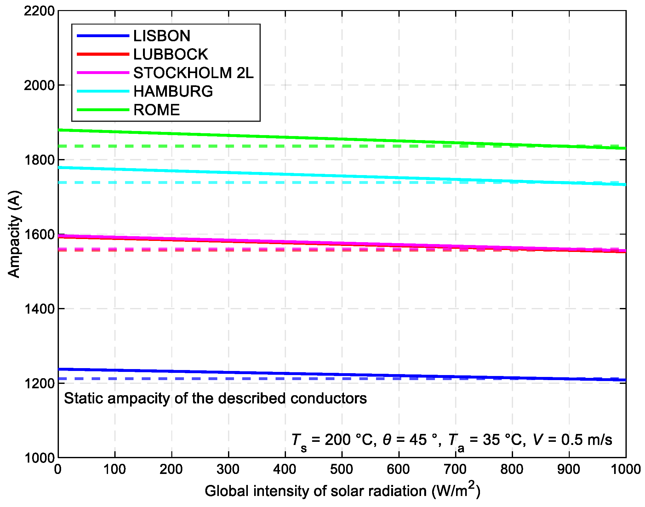
Figure 13.
Effect of current variation I on the temperature Ts of ACSR and ACCC conductors under SLR conditions (numerical method).
Figure 13.
Effect of current variation I on the temperature Ts of ACSR and ACCC conductors under SLR conditions (numerical method).
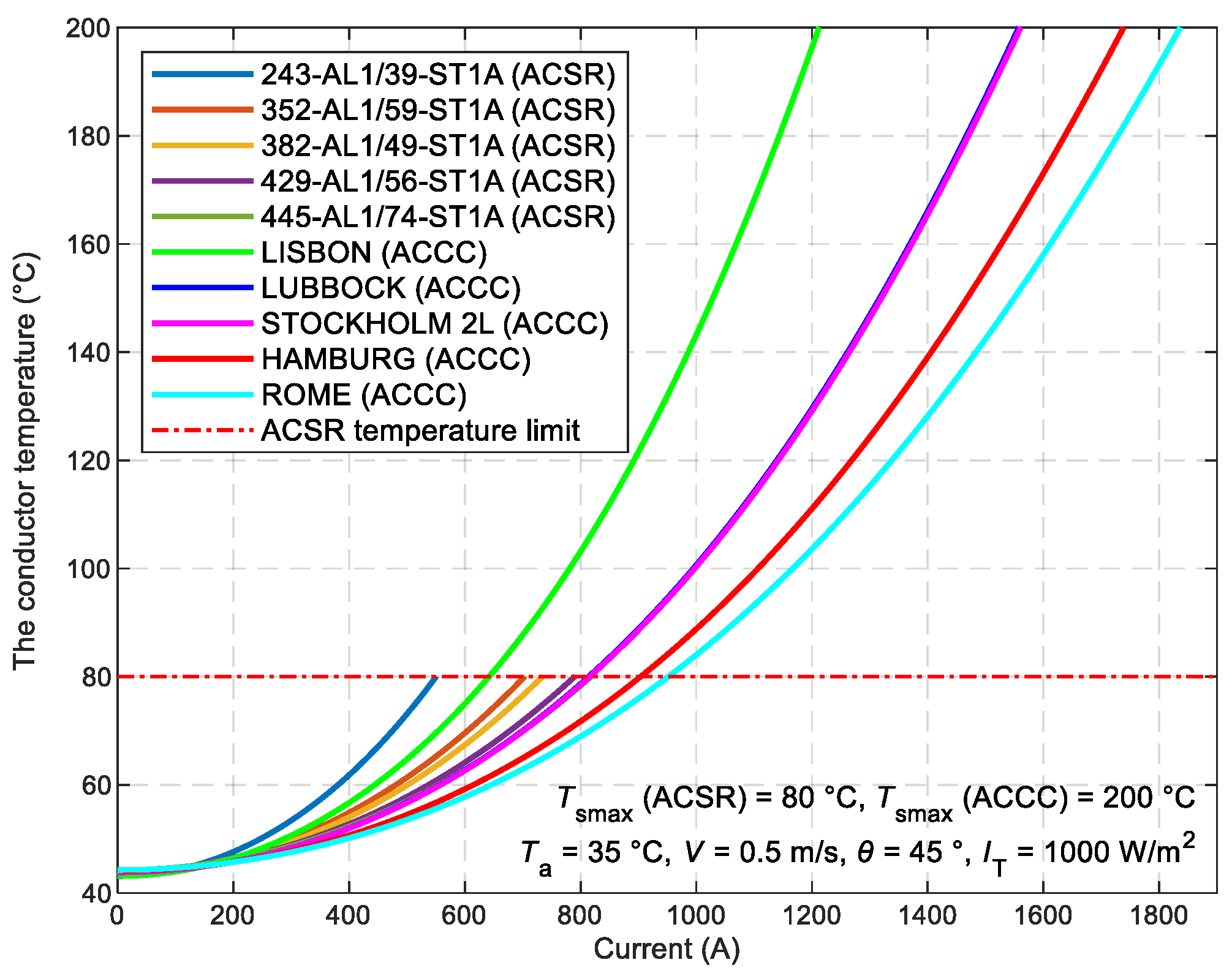
Figure 14.
Analysis of the dynamic steady-state ampacity Imax for transmission line V427 utilizing ACSR conductor 352-AL1/59-ST1A.
Figure 14.
Analysis of the dynamic steady-state ampacity Imax for transmission line V427 utilizing ACSR conductor 352-AL1/59-ST1A.
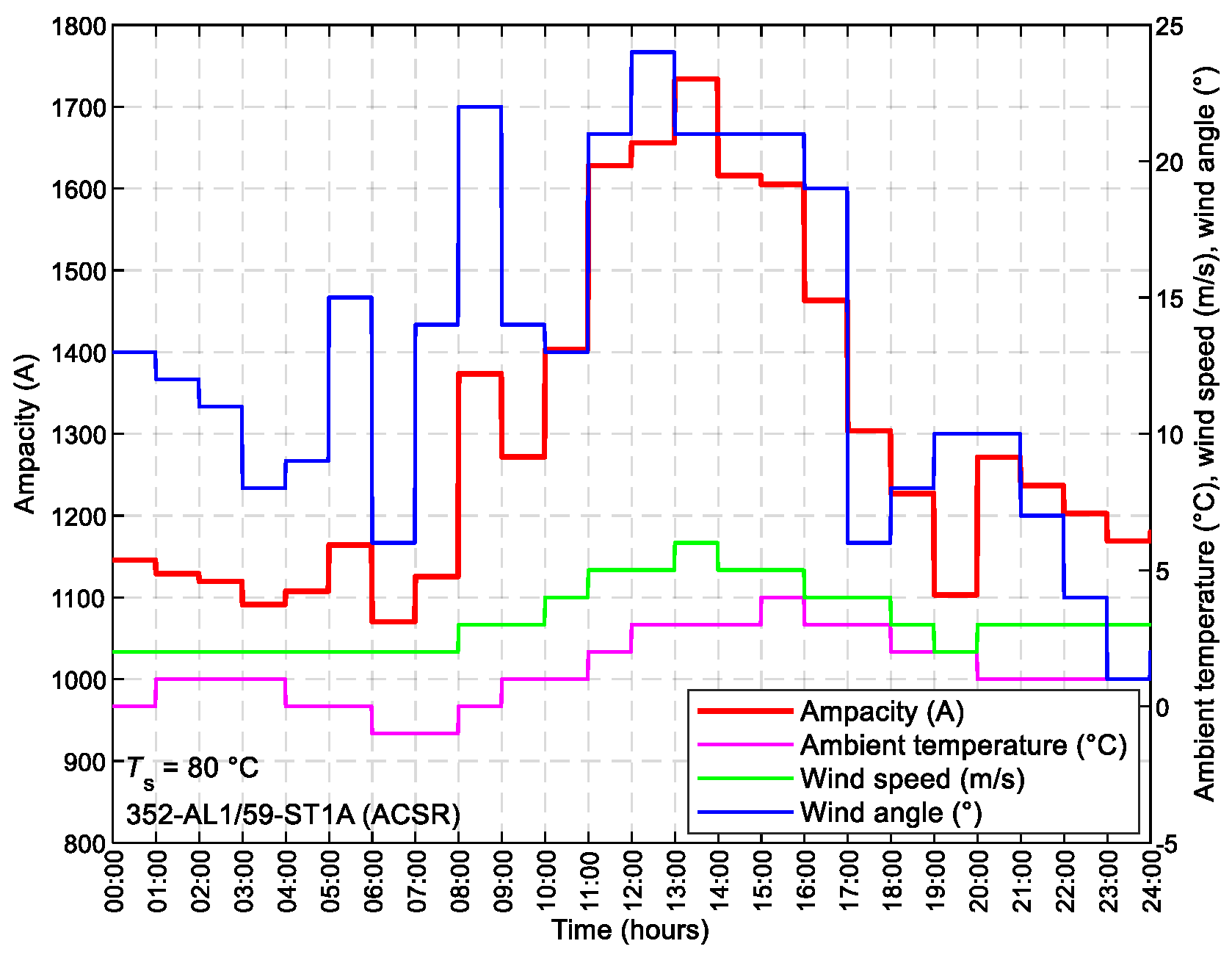
Figure 15.
ACCC conductor replacement impact on dynamic steady-state ampacity Imax analysis for transmission line V427.
Figure 15.
ACCC conductor replacement impact on dynamic steady-state ampacity Imax analysis for transmission line V427.
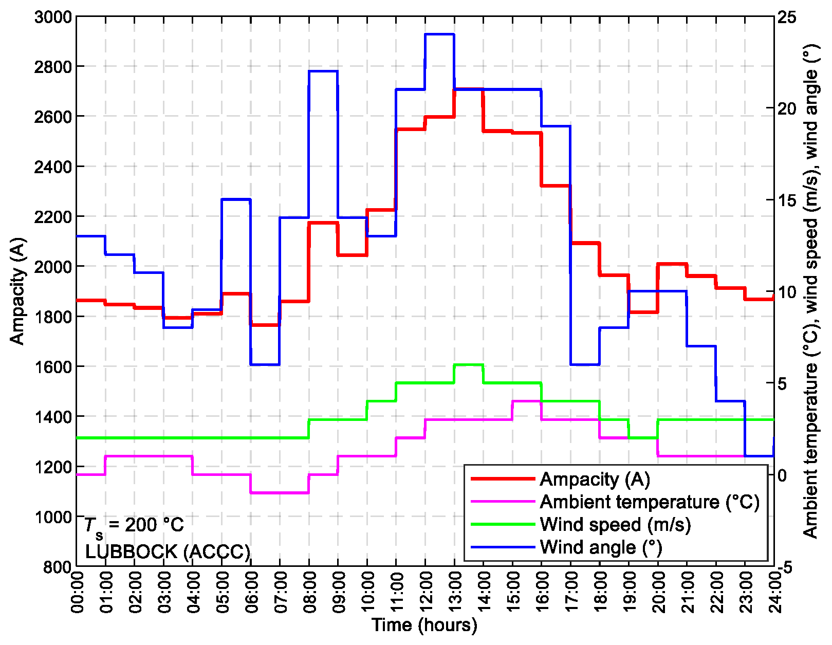

Table 1.
The fundamental types of HTLS conductors and their specifications [9].
Table 1.
The fundamental types of HTLS conductors and their specifications [9].
| Conductor designation | Conductor name | Maximum allowable temperature (°C) |
|---|---|---|
| ACSS | Aluminium conductor, steel supported | 200 – 250 |
| G(Z)TACSR | Gap type super thermal resistant aluminium alloy, steel reinforced | 150 – 210 |
| (Z)TACSR | Super thermal resistantaluminium alloy conductor, steel reinforced | 150 – 210 |
| (Z)TACIR | Super thermal resistantaluminium alloy conductor, invar reinforced | 150 – 210 |
| KTACSR | High strength thermal resistantaluminium alloy conductor, steel reinforced | 150 |
| ACCR | Aluminium conductor composite reinforced | 210 |
| ACCC | Aluminium conductor composite core conductors | 200 – 250 |
Table 2.
Technical specifications of the analysed ACSR conductors.
| Type of conductor | 243-AL1/39-ST1A | 352-AL1/59-ST1A | 382-AL1/49-ST1A | 429-AL1/56-ST1A | 445-AL1/74-ST1A | Type of conductor |
|---|---|---|---|---|---|---|
| Conductor diameter (mm) | 21.75 | 26.5 | 27.0 | 28.7 | 29.7 | Conductor diameter (mm) |
| Diameter of the aluminium wire in the aluminium conductor(mm) | 3.45 | 4.0 | 3.0 | 3.75 | 4.5 | Diameter of the aluminium wire in the aluminium conductor (mm) |
| Electrical resistance of the conductor (Ω/km) | 0.1181 | 0.0816 | 0.0650 | 0.0674 | 0.0758 | Electrical resistance of the conductor (Ω/km) |
| Thermal coefficient of resistance (K-1) | 4.03∙10-3 | |||||
| The absorptivity of the surface of the conductor (–) | 0.65 | |||||
| Emissivity coefficient of conductor surface (–) | 0.35 | |||||
Table 3.
The assessment of ampacity differences between ACSR and ACCC conductors at temperatures Ts of 80 and 200 °C (numerical method).
Table 3.
The assessment of ampacity differences between ACSR and ACCC conductors at temperatures Ts of 80 and 200 °C (numerical method).
| ACSR conductor | Ampacity (A)at Ts = 80 °C | ACCC conductor | Ampacity (A)at Ts = 80 °C | Ampacity (A) at Ts = 200 °C |
| 243-AL1/39-ST1A | 550.2 | LISBON | 641.7 | 1212.2 |
| 352-AL1/59-ST1A | 703.2 | LUBBOCK | 814.1 | 1557.4 |
| 382-AL1/49-ST1A | 733.9 | STOCKHOLM 2L | 815.9 | 1560.7 |
| 429-AL1/56-ST1A | 789.8 | HAMBURG | 903.8 | 1738.7 |
| 445-AL1/74-ST1A | 817.9 | ROME | 951.7 | 1836.4 |
Table 4.
Alternative replacement for ACSR conductors.
| ACSR conductor | 243-AL1/39-ST1A | 352-AL1/59-ST1A | 382-AL1/49-ST1A | 429-AL1/56-ST1A | 445-AL1/74-ST1A |
| Conductor diameter (mm) | 21.75 | 26.50 | 27.00 | 28.70 | 29.70 |
| Approx. weight (kg/km) | 980.1 | 1433.45 | 1442.5 | 1620.8 | 1831.81 |
| ACCC conductor | LISBON | LUBBOCK | STOCKHOLM 2L | HAMBURG | ROME |
| Conductor diameter (mm) | 21.79 | 26.42 | 26.39 | 28.63 | 29.90 |
| Approx. weight (kg/km) | 946 | 1375 | 1395 | 1627 | 1775 |
| Diameter of the aluminium wire in the aluminium conductor (mm) | 7.11 | 8.76 | 8.76 | 8.76 | 9.53 |
| Electrical resistance of the conductor (Ω/km) | 0.0887 | 0.0608 | 0.0605 | 0.0514 | 0.0474 |
Disclaimer/Publisher’s Note: The statements, opinions and data contained in all publications are solely those of the individual author(s) and contributor(s) and not of MDPI and/or the editor(s). MDPI and/or the editor(s) disclaim responsibility for any injury to people or property resulting from any ideas, methods, instructions or products referred to in the content. |
© 2024 by the authors. Licensee MDPI, Basel, Switzerland. This article is an open access article distributed under the terms and conditions of the Creative Commons Attribution (CC BY) license (http://creativecommons.org/licenses/by/4.0/).
Copyright: This open access article is published under a Creative Commons CC BY 4.0 license, which permit the free download, distribution, and reuse, provided that the author and preprint are cited in any reuse.


