Controlled Quantum Communication Using Quantum Random Walk

Subham Das; A.V.N.S. Meghanath; Rajiuddin Sk; Prasanta K. Panigrahi

doi:10.20944/preprints202405.2035.v1

Preprint

Article

Controlled Quantum Communication Using Quantum Random Walk

This version is not peer-reviewed.

Subham Das,A.V.N.S. Meghanath,

Rajiuddin Sk^*

,Prasanta K. Panigrahi

Subham Das,A.V.N.S. Meghanath,

Rajiuddin Sk^*

,Prasanta K. Panigrahi

This version is not peer-reviewed.

Downloads

232

Views

Comments

Submitted:

29 May 2024

Posted:

30 May 2024

You are already at the latest version

Abstract

In this paper, we introduce a novel controlled quantum communication protocol utilizing a quantum random walk involving one sender, one receiver, and multiple controllers. Inspired by classical random walk theory, quantum random walk serves as the foundation of our proposed protocol. With this protocol, we demonstrate the ability to transfer any n- dimensional quantum state to any party facilitated by any m number of controllers. Furthermore, any of the (m+1) individuals has the freedom to accept the role of the receiver. Rigorous testing of the protocol’s performance is conducted through quantum state tomography. We have run different variations of the circuits in IBMQ QASM simulator. Additionally, we explore the effectiveness of a weak measurement-based protocol designed to mitigate amplitude-damping noise’s detrimental effects on quantum states. By analyzing fidelity versus amplitude damping noise-strength plots for scenarios with and without the weak measurement protocol, we provide valuable insights into its protective capabilities across various levels of noise. These find- ings illuminate the protocol’s potential applications in quantum information processing

Keywords:

Quantum Random Walk

;

Controlled Quantumcommunication

;

Weak Measurement

Subject:

Physical Sciences - Quantum Science and Technology

1. Introduction

1.1. Quantum Communication

Quantum communication has sparked a revolution in conventional communication systems, offering unparalleled security measures. Beginning with the BB84 quantum key distribution protocol [1] and quantum teleportation protocol [2], quantum communication has made significant strides in its development and application. Recently, significant progress has been made in experimental quantum communication. Various quantum communication protocols, such as quantum key distribution [3], quantum teleportation [4], and superdense coding [5], have been experimentally validated using photonics or superconducting qubit. Recent advancements have witnessed the implementation of various quantum communication protocols on NISQ (Noisy Intermediate-Scale Quantum) devices [6,7,8,9].

Quantum communication can show a significant advantage against traditional communication methods that rely on classical information encoding, which can be vulnerable to eavesdropping and interception, posing significant risks to sensitive data and communications. One of the main reasons of this advantage of quantum communication is due to the presence of superposition and entanglement. These properties help us design protocols which either inform us about eavesdropping or make the system resistant to it, even if the original qubit source is untrusted. Moreover, the no-cloning theorem doesn’t allow the information to be copied, making the system far more secure than classical communication.

One of the big problems in classical Key distribution is generating the key to secure our communication. To address this problem, quantum key distribution (QKD) is proposed that uses the randomness of quantum measurement or the power of the maximally entangled states to generate the key for classical communication. In QKD, the presence of an eavesdropper can be easily detected by examining the correlations between the parties involved. Quantum random walk is currently being explored for quantum key generation, due to its intrinsically quantum characteristics [10].

1.2. Quantum Random Walk

A quantum random walk is considered a quantum analogue of classical random walks. In a classical random walk, a particle moves randomly according to certain probabilities [11]. Recent research on quantum random walks indicates that they may exhibit behaviour distinct from that of their classical counterparts [12,13,14]. Quantum Walk can be both discrete [12] and continuous time [15] version. Each version has brought a novel perspective to do quantum task [16]. In a quantum random walk, there is a coin space and a position space. In the first step, we use a unitary operator on the spin of the coin space and then apply a conditional shift operation on the position space. A minor change in the unitary operator of the coin space of the quantum walk can significantly change the output. In a quantum random walk, the particle starts in a superposition state and evolves governed by quantum operations. At each step, the particle’s state spreads out over multiple locations, creating interference patterns that can lead to different outcomes compared to classical random walks. This spread of states and interference effects are crucial for various quantum algorithms and quantum information processing tasks. The quantum random walk has found use in various areas [17,18,19]. In the following we will showcase its usefulness for quantum communication as also the use of weak measurement in protecting the quantum communication protocol against noise.

1.3. Weak Measurements

Weak measurement is a counter intuitive measurement protocol initially introduced by Aharonov, Albert, and Vaidman in 1988 who explore the efficiency of the weak measurement scheme against decoherence and this measurement scheme is now used to perform various tasks in the field of quantum information theory [20]. Weak measurement has a unique property, that it can extract information without completely disturbing the state, unlike strong measurements [21].

Weak measurements have found applications across various domains of quantum physics, including quantum information processing, quantum metrology, and fundamental tests of quantum mechanics. In quantum information processing, weak measurements play a crucial role in quantum state tomography, quantum error correction, and enhancing the efficiency of quantum algorithms. Moreover, in quantum metrology, weak measurements allow for the precise estimation of parameters with high sensitivity, surpassing the limitations imposed by classical measurement techniques [22].

In this paper, we propose a novel controlled quantum communication protocol using quantum random walk. We perform quantum tomography of the output state to calculate the fidelity. Furthermore, we perform a weak measurement-based protection protocol on a qubit designed to protect it from amplitude damping. A comparison is made on the performance of the protocol with and without the weak measurement-based protection protocol graphically.

1.4. Contributions of the Paper

The contributions of this paper can be summarized as follows:

We propose a controlled quantum communication protocol using quantum random walk that can teleport any N-dimensional quantum state.
The fidelity of the quantum states after quantum tomography for this protocol is high.
We present a comparative analysis between the protocol under amplitude damping and the performance of the protocol with weak measurement protocol in the presence of amplitude damping noise to showcase the usefulness of the weak measurement.

1.5. Organization

The structure of the paper is as follows: Section 2 covers related work. In Section 3, we describe the theoretical framework of the algorithms. Section 4 presents the results. Finally, Section 5 discusses the findings, concludes the paper, and suggests potential extensions for future research.

2. Related Works

In the teleportation protocol proposed in the paper [23]. A sender, Alice, successfully transmits an unknown state of a two-level particle to a remote receiver, Bob. This transmission is facilitated by a triplet of entangled particles initially shared and controlled by a supervisor, Charlie. In the paper [24], the researcher implements some perfect state transfer tasks on various graphs using quantum random walk. The work in this paper is inspired by the one-dimensional protocol proposed by Y. Chatterjee et al. [6]. They teleported qubits using quantum walk but did not have a controller. Furthermore, the circuits for transferring higher-dimensional qubits were not straightforward.

3. Theory

3.1. Quantum Random Walk

As mentioned earlier Quantum Random Walk (QRW) serves as a quantum counterpart to the classical random walk, wherein the evolution of a walker is governed by principles of quantum mechanics rather than classical probability distributions. A pivotal component in QRWs is the quantum coin flip, often realized through the application of a Hadamard gate. This gate creates a superposition of states analogous to “heads" and “tails", mimicking the randomness inherent in classical coin flips. In our proposed algorithm, we leverage this quantum coin flip methodology by employing a Hadamard gate on the coin qubit, followed by conditional operations on the walker qubit, typically implemented using controlled-NOT gates. These conditional operations dictate the walker’s movement based on the state of the coin qubit, analogous to the classical random walk’s directional shifts. The resultant quantum circuit facilitates the simulation of the walker’s probabilistic evolution, emulating classical random walks in a quantum framework.

3.2. Theoretical Framework of the Algorithm

Here We propose a controlled quantum communication protocol using a quantum random walk. The steps for the protocol can be summarized as follows:

For sending an N-dimensional quantum state with M number of controllers, we need M+2 number of N-dimensional coin space and one N-dimensional position space. Let the general state be $| ϕ 〉$ :

$| ϕ 〉 = \sum C_{i} | i 〉 .$

(1)
The first step is to apply the Hadamard gate on each qubit line of the quantum circuit except the sender state and position state. The operation leads to the state

$| ψ 〉 = ({| 0 〉}^{\otimes N} \otimes | ϕ 〉 \otimes ⨂_{j = 1}^{M} H^{\otimes N} {| 0_{j} 〉}^{\otimes N}) .$

(2)
The state ${| H 〉}^{\otimes N} {| 0_{j} 〉}^{\otimes N}$ can be expressed as

${| H 〉}^{\otimes N} {| 0_{j} 〉}^{\otimes N} = \frac{1}{\sqrt{2^{n}}} \sum_{n} | y_{j}^{n} 〉 .$

(3)

On using Eq. 3, the state 2 will become

$| ψ 〉 = {| 0 〉}^{\otimes N} \otimes \sum_{i} C_{i} | i 〉 \otimes \frac{1}{{\sqrt{2^{n}}}^{N / 2}} ⨂_{j = 1}^{M} \sum_{γ} {| y_{j}^{γ} 〉}^{\otimes N} .$

(4)
For sending the general N-dimensional quantum state, the sender applies the CNOT gate on the i-th qubit line of the position space as the i-th qubit line of the coin space of the sender as a controller for all N qubit lines of the sender. This step changes the position space state

$| ψ 〉 = \sum_{i} C_{i} | i 〉 \otimes | i 〉 \otimes \frac{1}{{\sqrt{2^{n}}}^{N / 2}} ⨂_{j = 1}^{M} \sum_{γ} {| y_{j}^{γ} 〉}^{\otimes N} .$

(5)
For convenience, we will drop the normalisation coefficient. The receiver and controllers do the same CNOT gate on the i-th qubit line of the position space as the i-th qubit line of the coin space of the member as a controller for all N qubit lines of the sender:

$| ψ 〉 = \sum_{γ} \sum_{i} C_{i} | i \oplus \sum_{j = 1}^{M} y_{j}^{γ} 〉 \otimes | i 〉 \otimes {(⨂_{j = 1}^{M} | y_{j}^{γ} 〉)}^{\otimes N}$

(6)
The sender then applies the Hadamard gate on each qubit line of the sender. This step produces our resource state, which has the following form

$\begin{matrix} | ψ 〉 = \sum_{γ} \sum_{i} \sum_{α} C_{i} | i \oplus \sum_{j = 1}^{M} y_{j}^{γ} 〉 \otimes {(- 1)}^{α . i} | α 〉 \otimes {(⨂_{j = 1}^{M} | y_{j}^{γ} 〉)}^{\otimes N} . \end{matrix}$

(7)

Note that we can simplify the protocol by restricting the value of M to 1, creating a basic sender and receiver system without controllers.
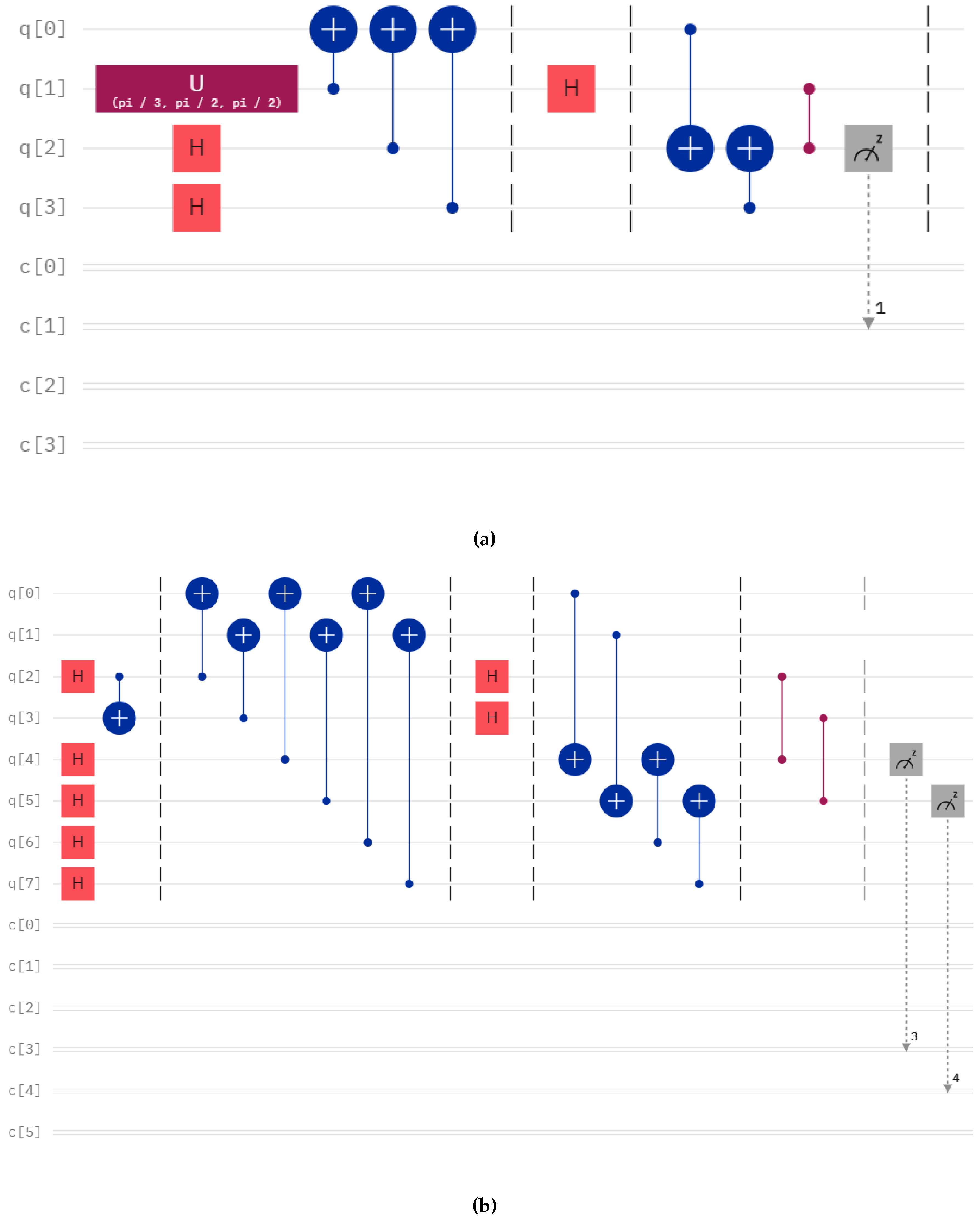
The sender will now perform measurements on the coin space and the position space using a computational basis. Let us call this output M1 and M2. Each of the sets has N number of elements made of 0 and 1. This number corresponds to the state in which the resource state has collapsed. The sender sends this value to the receiver via classical communication. Similarly, all the controllers perform such measurements and send them to the receiver via classical communication. Based on the output, the receiver performs gate operations on his quantum state, thus retracting the original state. We have shown the quantum circuit diagram for single qubit teleportation with different controllers in Figure 1. Similarly, the corresponding quantum circuit for teleportation of two and three qubits is given in Figure 7 and Figure 8 in Appendix.

3.3. Receiver Operation

The General operation rule before doing the measurement for the receiver can be understood through this analysis. The state that was produced was a superposition state of this term:

| χ 〉 = C_{i} | i \oplus \sum_{j = 1}^{M} y_{j}^{γ} 〉 \otimes {(- 1)}^{α . i} | α 〉 \otimes {(⨂_{j = 1}^{M} | y_{j}^{γ} 〉)}^{\otimes N} .

(8)

If we want the j=1 case as the receiver and others of the M as controllers, then the desired state should be

| χ 〉 = C_{i} | i \oplus \sum_{j = 1}^{M} y_{j}^{γ} 〉 \otimes {(- 1)}^{α . i} | α 〉 \otimes | y_{1}^{γ} 〉 \otimes {(⨂_{j = 2}^{M} | y_{j}^{γ} 〉)}^{\otimes N} .

(9)

To generate the state for the receiver, we perform the CNOT operation with a controller on the position space and on the controller coin space. The resultant state is given by

| χ 〉 = | i \oplus \sum_{j = 1}^{M} y_{j}^{γ} 〉 \otimes | α 〉 \otimes {(- 1)}^{α . i} C_{i} | i 〉 \otimes {(⨂_{j = 2}^{M} | y_{j}^{γ} 〉)}^{\otimes N} .

(10)

The resource state has an extra term

{(- 1)}^{α . i}

, which can be removed by a controlled Z operation. This leads to

| χ 〉 = | i \oplus \sum_{j = 1}^{M} y_{j}^{γ} 〉 \otimes | α 〉 \otimes C_{i} | i 〉 \otimes {(⨂_{j = 2}^{M} | y_{j}^{γ} 〉)}^{\otimes N} .

(11)

Now, let us substitute the summation symbol to produce the resultant state. This step is ready to be measured by the receiver. Hence, the above equation takes the following form:

| ψ 〉 = \sum_{γ} \sum_{i} \sum_{α} | χ 〉 .

(12)

| ψ 〉 = \sum_{γ} \sum_{i} \sum_{α} | i \oplus \sum_{j = 1}^{M} y_{j}^{γ} 〉 \otimes | α 〉 \otimes C_{i} | i 〉 \otimes {(⨂_{j = 2}^{M} | y_{j}^{γ} 〉)}^{\otimes N} .

(13)

Through this analysis, we concluded that the receiver’s operation on each qubit line is contingent upon the sender’s coin space, position space measurement output and the controller’s coin space output. Specifically, if the sender obtains a 1 as the output for the i-th qubit in the coin space, the receiver performs a Z gate operation on the i-th qubit line. If the sender’s output corresponds to 1 in the position space, the receiver performs an X gate operation. Additionally, for the controller’s measurement outcomes on the i-th qubit, if the outcome is 1, the receiver applies an X gate operation.

3.4. Communication between Symmetrical and Asymmetrical Coin space

The communication protocol given here demands the receiver and the sender coin space to be of the same dimension. However, it is possible to communicate between coin spaces that are not equal by reducing the dimension of the coin space by using entanglement. Exploiting this property, we can communicate between asymmetrical coin spaces. An example circuit is shown in Figure 2.

3.5. Amplitude Damping

In the realm of quantum computing, amplitude damping is a crucial quantum error that can lead to the loss of quantum information. This phenomenon occurs when a qubit, representing a quantum state, interacts with its environment, causing the qubit’s amplitude to decay. Amplitude damping is primarily observed in quantum systems where the qubits are susceptible to energy dissipation. Amplitude damping is commonly quantified using Kraus operators, which describe the evolution of the quantum state when subjected to noise. For amplitude damping, the Kraus operators are given by

\begin{matrix} E_{0} = & \sqrt{p} | 0 〉 〈 1 |, \\ E_{1} = & | 0 〉 〈 0 | + \sqrt{1 - p} | 1 〉 〈 1 | . \end{matrix}

This map can also be represented in the following form:

\begin{matrix} {| 0 〉}_{s} {| 0 〉}_{E} & ⟶ {| 0 〉}_{s} {| 0 〉}_{E}, \\ {| 1 〉}_{s} {| 0 〉}_{E} & ⟶ \sqrt{1 - p} {| 1 〉}_{s} {| 0 〉}_{E} + \sqrt{p} {| 0 〉}_{s} {| 0 〉}_{E} . \end{matrix}

(14)

3.6. Weak Measurement Based Protection Protocol

Weak measurement has found uses in protecting the quantum state from amplitude damping Noise. The protocol given in the paper [25] is used to protect the state from decoherence. The steps involved in the process are

Step 1: Weak Measurement

In the initial step, weak measurements are applied to gain partial information about the system. These measurements are characterized by operators $Π_{0} = M_{0}^{†} M_{0}$ and $Π_{1} = M_{1}^{†} M_{1}$ , oriented along the z-axis of the Bloch sphere. The operators $M_{0}$ and $M_{1}$ are defined as follows:

$M_{0} = cos (θ / 2) | 0 〉 〈 0 | + sin (θ / 2) | 1 〉 〈 1 | M_{1} = sin (θ / 2) | 0 〉 〈 0 | + cos (θ / 2) | 1 〉 〈 1 | .$

Here, $θ$ dictates the measurement’s strength, with three distinct schemes: “no measurement" (NM) when $θ = \frac{π}{2}$ , “projective measurement" (PM) when $θ = 0$ , and “weak measurement" (WM) when $0 < θ < \frac{π}{2}$ .
Step 2: Offsetting Operations

Following the measurement, corrective operations are enacted to counteract noise effects before amplitude damping (ADC). These operations, denoted as $F_{0}$ and $F_{1}$ , are determined by the measurement outcomes:

$F_{0} = I = (\begin{matrix} 1 & 0 \\ 0 & 1 \end{matrix}), F_{1} = σ_{x} = (\begin{matrix} 0 & 1 \\ 1 & 0 \end{matrix})$

Where $F_{0}$ corresponds to the result of $M_{0}$ and $F_{1}$ corresponds to the result of $M_{1}$ .
Step 3: Amplitude Damping Correction

In this phase, the system is readied for ADC by addressing amplitude damping using Kraus operators for each qubit:

$E_{0} = (\begin{matrix} 1 & 0 \\ 0 & \sqrt{1 - r} \end{matrix}), E_{1} = (\begin{matrix} 0 & \sqrt{r} \\ 0 & 0 \end{matrix}) .$

Here, $r \in [0, 1]$ represents the probability of decay from the excited state, determined by $r = e^{- Γ t}$ , where $Γ$ is the energy relaxation rate and t is the evolution time. Note that the r mentioned here is same as the p mentioned in Section 3.5.
Step 4: Post-Amplitude Damping Correction

Following ADC, the same offsetting operations from Step 2 are applied.
Step 5: Correction Rotation

Finally, correction rotations are implemented to restore the state to its initial condition. These rotations, $T_{0}$ and $T_{1}$ , are applied based on the measurement outcomes:

$T_{0} = (\begin{matrix} e^{i η / 2} & 0 \\ 0 & e^{- i η / 2} \end{matrix}), T_{1} = (\begin{matrix} e^{- i η / 2} & 0 \\ 0 & e^{i η / 2} . \end{matrix})$

Where $T_{0}$ corresponds to the result of $M_{0}$ and $T_{1}$ corresponds to the result of $M_{1}$ . The value of $η$ is given by

$\begin{matrix} η_{opt}^{p} (τ, θ) = \\ - i log (\frac{1 + \sqrt{1 - 4 ({cos}^{2} (θ / 2) + r {sin}^{2} (θ / 2)) ((1 - r) {sin}^{2} (θ / 2))}}{2 ({cos}^{2} (θ / 2) + r {sin}^{2} (θ / 2))}) . \end{matrix}$

(15)

This protocol systematically shields the quantum Fisher information of the N-qubit GHZ state from decoherence by integrating weak measurements, corrective operations, amplitude damping correction, and correction rotations. Adjusting the measurement strength allows for a balance between information acquisition and disturbance minimization.

3.7. Quantum State Tomography

Quantum state tomography is a powerful technique used to reconstruct unknown quantum states by performing measurements on an ensemble of identically prepared quantum systems. In quantum mechanics, a quantum state is fully characterized by a density matrix, which encapsulates all information about the system’s state, including its superposition and entanglement properties. The process of quantum state tomography involves preparing a large number of identical quantum systems in the same initial state, subjecting them to a series of measurements in different bases, and then using the statistics of these measurements to infer the underlying quantum state. By collecting sufficient measurement data, researchers can reconstruct the density matrix with high fidelity, providing a complete description of the quantum state. For a single qubit, the equation for constructing the experimental density matrix

ρ_{E}

is given as follows:

\begin{matrix} ρ_{E} & = \frac{1}{2} (〈 X 〉 X + 〈 Y 〉 Y + 〈 Z 〉 Z + I) . \end{matrix}

(16)

Here, X, Y and Z correspond to the

\begin{matrix} I & = (\begin{matrix} 1 & 0 \\ 0 & 1 \end{matrix}), X = (\begin{matrix} 0 & 1 \\ 1 & 0 \end{matrix}), \\ Y & = (\begin{matrix} 0 & - i \\ i & 0 \end{matrix}), Z = (\begin{matrix} 1 & 0 \\ 0 & - 1 \end{matrix}) . \end{matrix}

The

〈 X 〉

〈 Y 〉

, and

〈 Z 〉

are expectation values calculated for this basis.

The general form of the two-qubit density matrix using expectation values is:

\begin{matrix} ρ & = \frac{1}{4} (I \otimes I + \sum_{i = 1}^{3} 〈 σ_{i} σ_{i} 〉 (σ_{i} \otimes σ_{i}) + \sum_{i = 1}^{3} \sum_{j \neq i} 〈 σ_{i} σ_{j} 〉 (σ_{i} \otimes σ_{j})) . \end{matrix}

(17)

where

σ_{i}

are the Pauli matrices:

\begin{matrix} σ_{0} & = I, σ_{1} = X, \\ σ_{2} & = Y, σ_{3} = Z \end{matrix}

and ⊗ represents the tensor product.

3.8. Quantum Fidelity

Quantum fidelity is a fundamental concept in quantum mechanics that quantifies the similarity between two quantum states [26]. It serves as a measure of how well one quantum state can be transformed into another while preserving its essential features. Mathematically, the fidelity

F (ρ, σ)

between two quantum states represented by density matrices

ρ

and

σ

is defined as the squared overlap between them:

\begin{matrix} F (ρ, σ) = Tr {(\sqrt{\sqrt{ρ} σ \sqrt{ρ}})}^{2} . \end{matrix}

(18)

Here, Tr denotes the trace operation, and

\sqrt{ρ}

and

\sqrt{σ}

represent the square roots of the density matrices.

High fidelity indicates a strong resemblance between the states, implying that they are nearly indistinguishable. In contrast, low fidelity signifies significant deviations or differences between the states.

3.9. Attack Analysis

The system is safe from external attack, as the protocol as for transferring N dimensional qubit, with m controller with symmetrical coin space. For Eve to extract the state, she has to guess the operation correctly. And the probability of guessing the operation correctly is

{(1 / 2)}^{(m + 2) n}

. Moreover, the protocol is secure against various external attacks like intercept-resend attacks, measurement-based attacks and measurement-resend attacks. attack

4. Experimental Results

4.1. Circuits Output on Simulators

We teleport different numbers of qubits with different numbers of controllers using our protocol using IBMQ QASM Simulator of IBM for 8193 shots. The diagram of those circuits are given in Figure 1, Figure 7 and Figure 8. We present the output of the run of those circuits on Table 1, Table 2 and Table 3 for different numbers of controllers and senders.

4.2. Results of Quantum State Tomography

In this section, we discuss the results of quantum state tomography to check how well the quantum states are teleported in our algorithm. We checked the performance of two circuits. The circuits used for the tomography are given in Figure 4. The theoretical density matrix is calculated using:

\begin{matrix} ρ_{t} = | ψ 〉 〈 ψ | . \end{matrix}

(19)

For one qubit and one controller circuit, we teleport

\frac{\sqrt{3}}{2} | 0 〉 + \frac{ι}{2} | 1 〉

in IBM Sherbrooke for 8193 shots generate by action of

U 3 (π / 3, π / 2, π / 2)

. The theoretical density matrix of the state is

ρ_{t} = [\begin{matrix} \frac{3}{4} & - \frac{\sqrt{3} i}{4} \\ \frac{\sqrt{3} i}{4} & \frac{1}{4} \end{matrix}] .

The experimental density matrix given in equation 16 for a single qubit after substituting matrices X, Y, and Z, the Pauli matrices, and

I

which is the identity matrix, we get:

ρ_{E} = \frac{1}{2} [\begin{matrix} 1 + 〈 Z 〉 & 〈 X 〉 - i 〈 Y 〉 \\ 〈 X 〉 + i 〈 Y 〉 & 1 - 〈 Z 〉 \end{matrix}] .

(20)

The expectation values was found out to be

〈 Z 〉 = 0.433

〈 X 〉 = - 0.109

, and

〈 Y 〉 = 0.674

, substituting the values, we get:

ρ_{E} = [\begin{matrix} 0.7165 & - 0.0545 - 0.337 i \\ - 0.0545 + 0.337 i & 0.2835 \end{matrix}] .

(21)

The fidelity achieved for this circuit was found out to be 0.81.

For two qubit state, we teleport the Bell state

| ϕ^{+} 〉

, the theoretical density matrix is

ρ_{Φ^{+}} = | Φ^{+} 〉 〈 Φ^{+} | = \frac{1}{2} (\begin{matrix} 1 & 0 & 0 & 1 \\ 0 & 0 & 0 & 0 \\ 0 & 0 & 0 & 0 \\ 1 & 0 & 0 & 1 \end{matrix}) .

(22)

For the Bell state, the experimental density matrix state is calculated using the IBM Brisbane processor of IBM Quantum computer using equation 17. The density matrix

ρ_{E}

is given in Eq. 23.

\begin{matrix} ρ_{E} = (\begin{matrix} 0.252 & 0.052 + 0.004 i & 0.102 - 0.009 i & 0.185 - 0.045 i - 0.018 i \\ 0.052 + 0.004 i & 0.247 & 0.173 + 0.009 i + 0.045 i & 0.102 - 0.009 i \\ 0.102 + 0.009 i & 0.173 - 0.009 i - 0.045 i & 0.247 & 0.052 - 0.004 i \\ 0.185 + 0.045 i + 0.018 i & 0.102 + 0.009 i & 0.052 + 0.004 i & 0.252 \end{matrix}) . \end{matrix}

(23)

The protocol achieved a fidelity of 0.61 for teleporting the Bell state.

Figure 3. Experimental density matrix plot for (a) single qubit and (b) two-qubit teleportation with one controller.

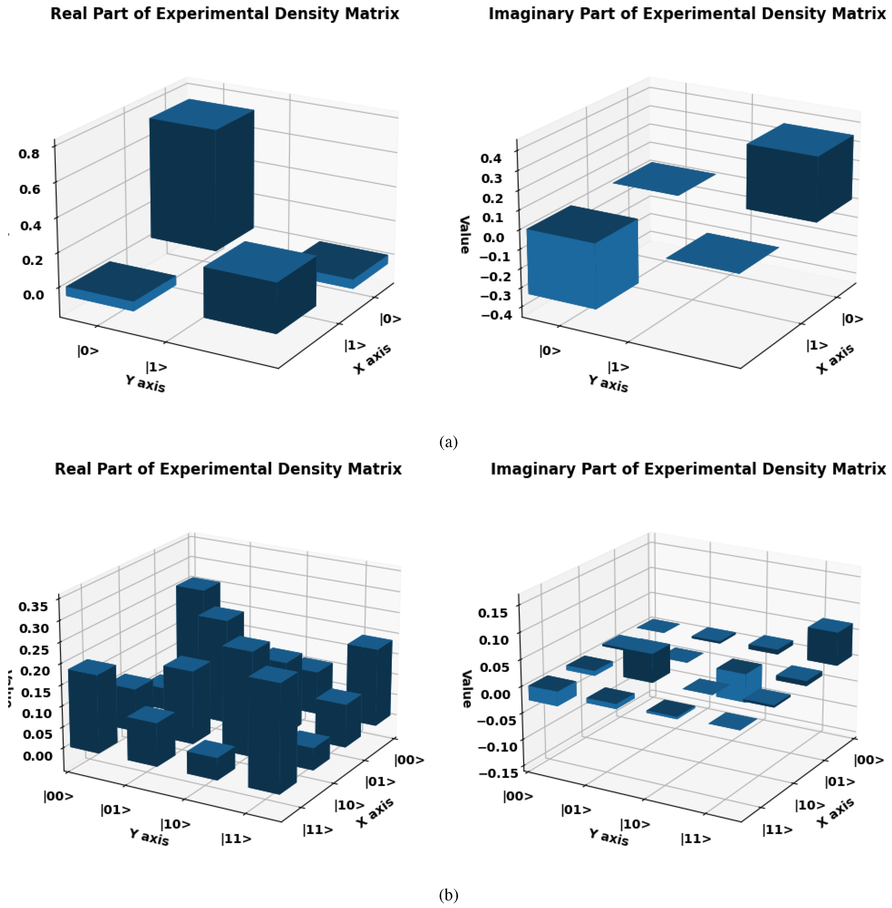
Figure 4. Circuit for teleportation of Bell states with one controller and one receiver. We calculated the fidelity for this circuit in IBM-Q of IBM Quantum Computer.

4.3. Results of Weak Measurements

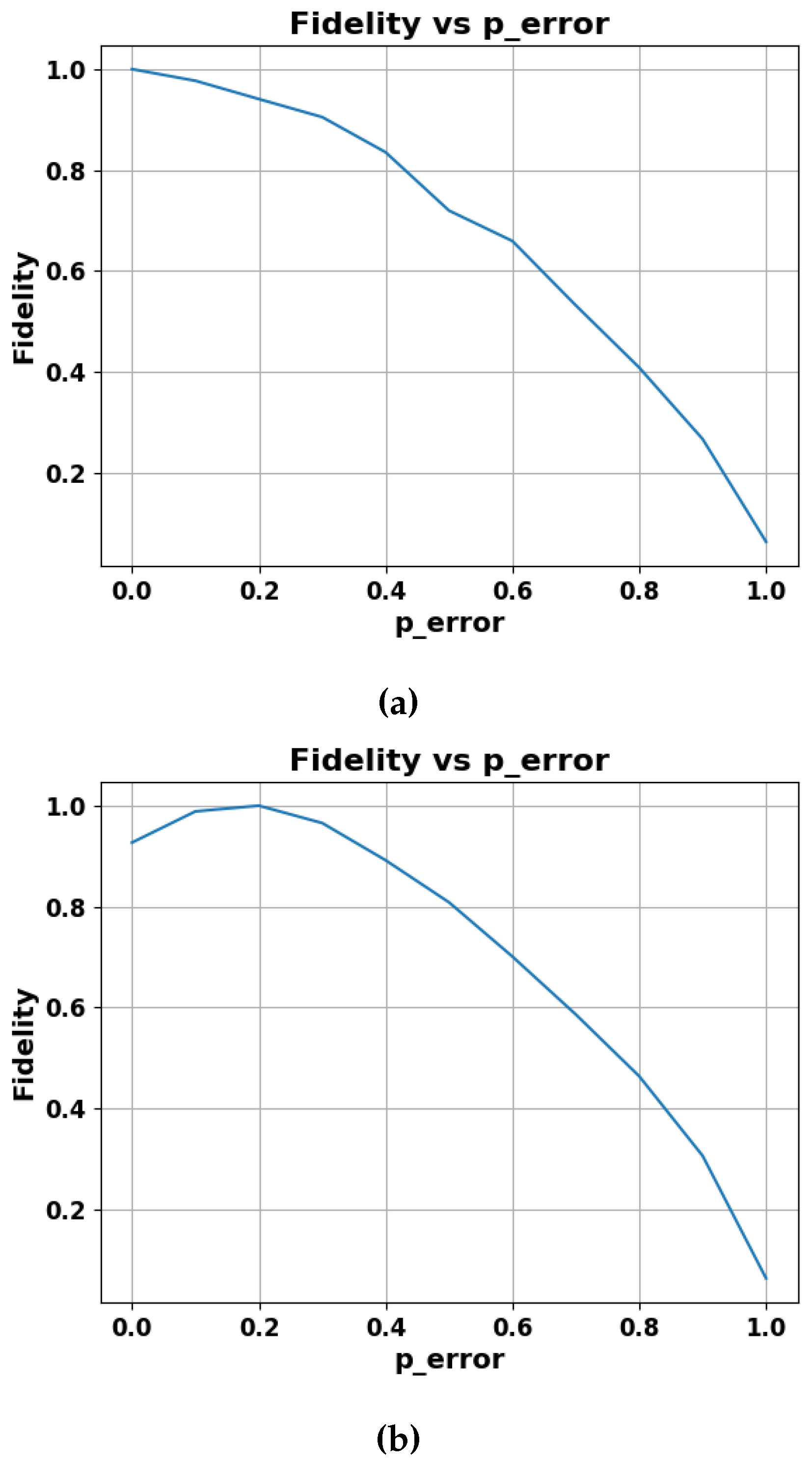
We investigate a weak measurement protocol’s ability to protect quantum states from amplitude-damping noise. Fidelity versus noise strength (p-error) graphs are presented for two scenarios: utilizing the weak testing protocol and not using it. Moreover, we illustrate the probability of the state

| 0 〉

(Prob-0) against noise strength (p-error), where p-error represents the intensity of amplitude damping. Our results provide insights into the effectiveness of the protocol in mitigating different levels of amplitude damping. The weak measurement strength implemented in the protocol was

π / 3

. In Figure 6, Figure 6a demonstrates the performance of the communication protocol without the weak measurement-based protocol under the influence of amplitude damping, while Figure 6b presents the performance of the communication protocol after implementing the Weak measurement protocol. Clearly, the protocol with Weak measurement maintained a higher Fidelity compared to the protocol under the influence of noise levels represented by p-error or p-values within the range from 0 to 0.5.

Figure 5. The plot illustrates the probability of obtaining the

| 0 〉

state as a function of the increasing p-value of amplitude damping, clearly indicating the slow decay rate of fidelity in presence of weak measurement.

Figure 5. The plot illustrates the probability of obtaining the

| 0 〉

state as a function of the increasing p-value of amplitude damping, clearly indicating the slow decay rate of fidelity in presence of weak measurement.

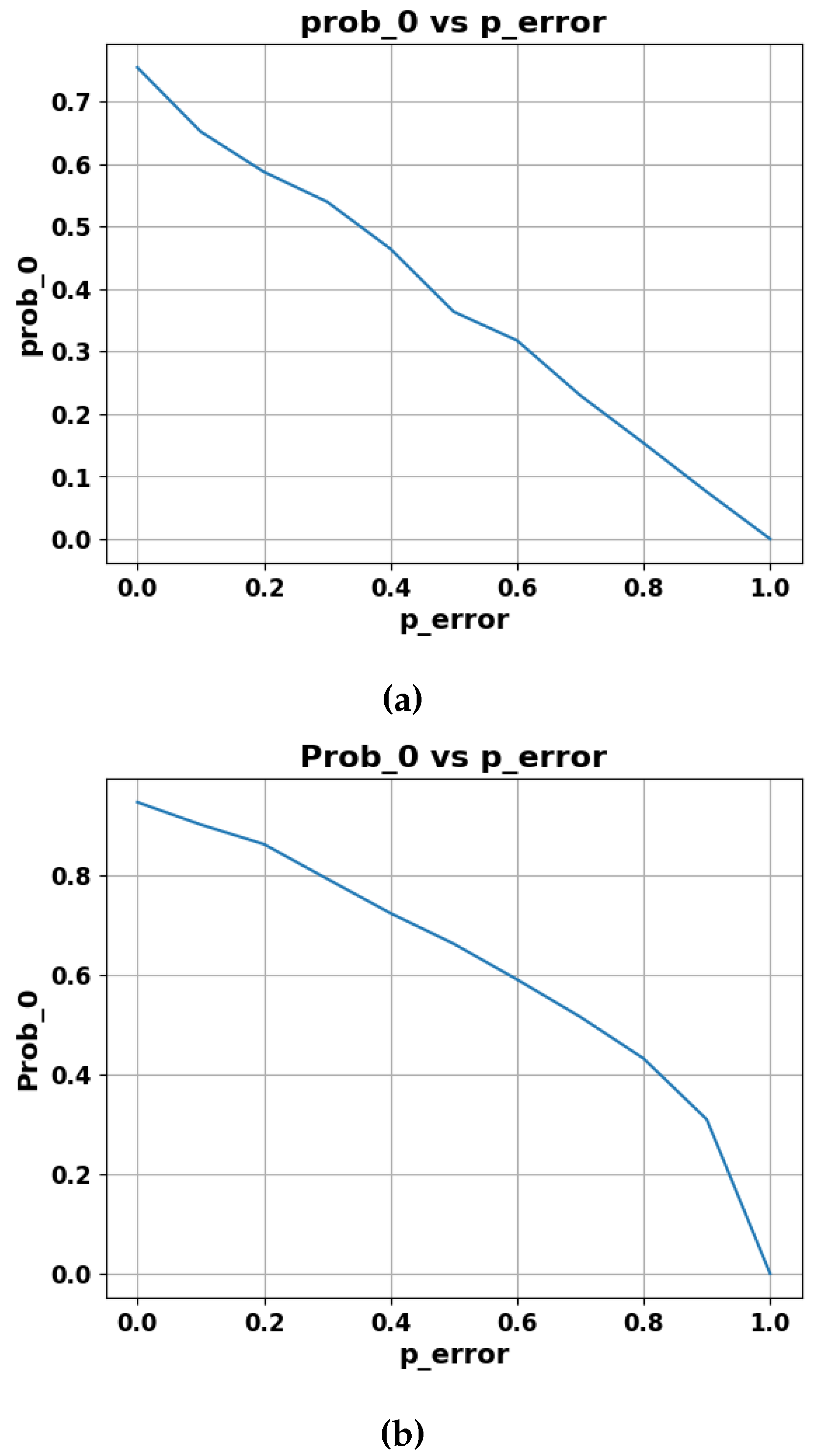
Figure 6. The plot illustrates fidelity with respect to increasing p-value of the amplitude damping.

5. Discussion and Conclusion

In our study, we have introduced a controlled quantum communication protocol designed for general N-dimensional quantum states with multiple controllers. Additionally, we have proposed modifications to facilitate communication between symmetrical and asymmetrical coin spaces. The protocol is implemented on the IBM QASM simulator, varying the number of controllers and qubits.

We have evaluated the fidelity of the protocol, which exhibits high fidelity in both single-qubit and two-qubit circuits governed by a single controller. Furthermore, we investigated the efficacy of a weak measurement-based protection protocol tailored to shield qubits against amplitude damping. This protection protocol was assessed using a single-qubit circuit with a single controller.

Our evaluation included graphical representations of performance outcomes in terms of the p-value, indicating the strength of amplitude damping. Our results encompass a comparative analysis demonstrating the protocol’s performance in environments with and without amplitude noise. Notably, the weak measurement-based protection protocol exhibited exceptional performance within the range of p-values from 0 to 0.5.

Acknowledgments

We extend our sincere appreciation to OpenAI’s ChatGPT for its invaluable assistance in refining sentence structures and rectifying grammatical errors throughout the course of this research paper. Additionally, we would like to express our gratitude to the I-HUB Quantum Technology Foundation for issuing the award letter for the Chanakya scholarship during both the mid and end phases of the project. Furthermore, we extend our thanks to IBM for providing us with the opportunity to utilize their quantum computers to calculate the fidelity of our protocols.

Appendix

Here, we provide the quantum circuit for the teleportation of two and three-qubit states with the assistance of single and multiple controllers, which are given in Figure 7 and Figure 8.

Figure 7. Circuit for teleportation of two-qubit states with (a) one controller, (b) two controllers, (c) three controllers.

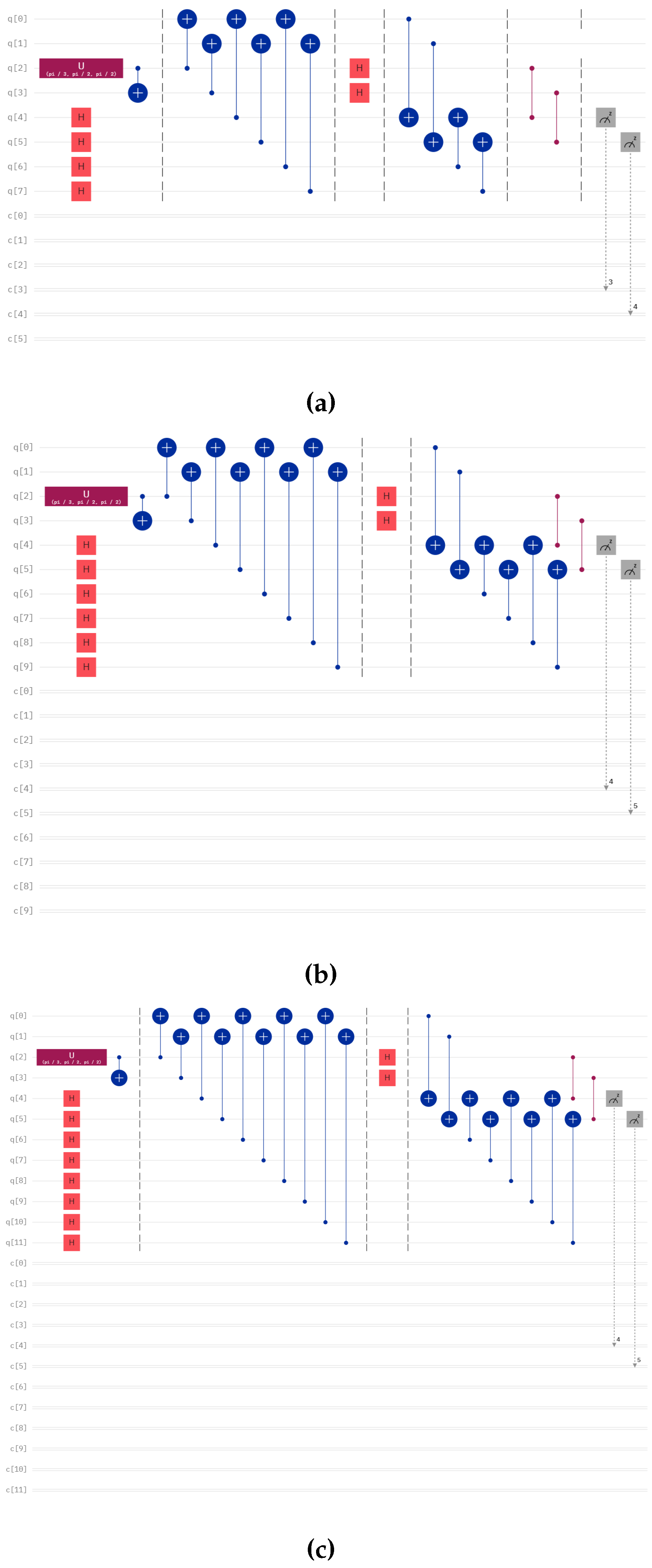
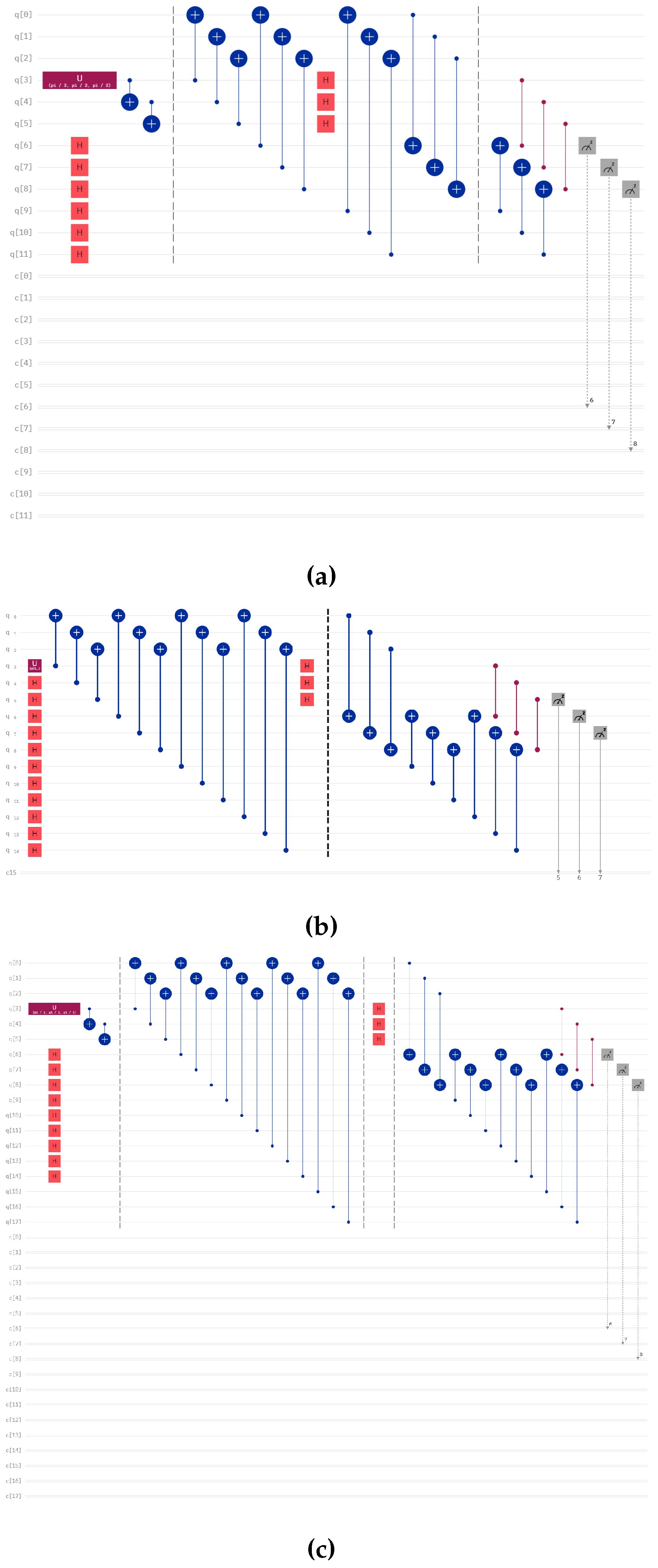
Figure 8. Circuit for teleportation of three-qubit state with (a) one controller, (b) two controllers, (c) three controllers.

References

Bennett, C.H.; Brassard, G. Quantum cryptography: Public key distribution and coin tossing. Theoretical computer science 2014, 560, 7–11. [Google Scholar] [CrossRef]
Bennett, C.H.; Brassard, G.; Crépeau, C.; Jozsa, R.; Peres, A.; Wootters, W.K. Teleporting an unknown quantum state via dual classical and Einstein-Podolsky-Rosen channels. Physical review letters 1993, 70, 1895. [Google Scholar] [CrossRef] [PubMed]
Zhao, Y.; Qi, B.; Ma, X.; Lo, H.K.; Qian, L. Experimental quantum key distribution with decoy states. Physical review letters 2006, 96, 070502. [Google Scholar] [CrossRef] [PubMed]
Bouwmeester, D.; Pan, J.W.; Mattle, K.; Eibl, M.; Weinfurter, H.; Zeilinger, A. Experimental quantum teleportation. Nature 1997, 390, 575–579. [Google Scholar] [CrossRef]
Williams, B.P.; Sadlier, R.J.; Humble, T.S. Superdense coding over optical fiber links with complete Bell-state measurements. Physical review letters 2017, 118, 050501. [Google Scholar] [CrossRef] [PubMed]
Chatterjee, Y.; Devrari, V.; Behera, B.K.; Panigrahi, P.K. Experimental realization of quantum teleportation using coined quantum walks. Quantum Information Processing 2019, 19. [Google Scholar] [CrossRef]
Rajiuddin, S.; Baishya, A.; Behera, B.K.; Panigrahi, P.K. Experimental realization of quantum teleportation of an arbitrary two-qubit state using a four-qubit cluster state. Quantum Information Processing 2020, 19, 1–13. [Google Scholar] [CrossRef]
Sk, R.; Dash, T.; Panigrahi, P.K. Quantum information splitting of an arbitrary three-qubit state by using three sets of GHZ states. IET Quantum Communication 2021, 2, 122–135. [Google Scholar] [CrossRef]
Sisodia, M.; Shukla, A.; Thapliyal, K.; Pathak, A. Design and experimental realization of an optimal scheme for teleportation of an n-qubit quantum state. Quantum Information Processing 2017, 16, 1–19. [Google Scholar] [CrossRef]
Sarkar, A.; Chandrashekar, C. Multi-bit quantum random number generation from a single qubit quantum walk. Scientific reports 2019, 9, 12323. [Google Scholar] [CrossRef]
Kempe, J. Quantum random walks: An introductory overview. Contemporary Physics 2003, 44, 307–327. [Google Scholar] [CrossRef]
Aharonov, Y.; Davidovich, L.; Zagury, N. Quantum random walks. Phys. Rev. A 1993, 48, 1687–1690. [Google Scholar] [CrossRef]
Childs, A.M.; Farhi, E.; Gutmann, S. An example of the difference between quantum and classical random walks. Quantum Information Processing 2002, 1, 35–43. [Google Scholar] [CrossRef]
Shenvi, N.; Kempe, J.; Whaley, K.B. Quantum random-walk search algorithm. Phys. Rev. A 2003, 67, 052307. [Google Scholar] [CrossRef]
Farhi, E.; Gutmann, S. Quantum computation and decision trees. Physical Review A 1998, 58, 915. [Google Scholar] [CrossRef]
Venegas-Andraca, S.E. Quantum walks: a comprehensive review. Quantum Information Processing 2012, 11, 1015–1106. [Google Scholar] [CrossRef]
Qu, D.; Matwiejew, E.; Wang, K.; Wang, J.; Xue, P. Experimental implementation of quantum-walk-based portfolio optimization. Quantum Science and Technology 2024, 9, 025014. [Google Scholar] [CrossRef]
Razzoli, L.; Cenedese, G.; Bondani, M.; Benenti, G. Efficient Implementation of Discrete-Time Quantum Walks on Quantum Computers. Entropy 2024, 26. [Google Scholar] [CrossRef]
Shi, W.M.; Xu, F.X.; Zhou, Y.H.; Yang, Y.G. A Novel Image Segmentation Algorithm based on Continuous-Time Quantum Walk using Superpixels. International Journal of Theoretical Physics 2023, 63, 4. [Google Scholar] [CrossRef]
Aharonov, Y.; Albert, D.Z.; Vaidman, L. How the result of a measurement of a component of the spin of a spin-1/2 particle can turn out to be 100. Physical review letters 1988, 60, 1351. [Google Scholar] [CrossRef] [PubMed]
Modak, N.; Singh, A.K.; Guchhait, S.; BS, A.; Pal, M.; Ghosh, N. Weak measurements in nano-optics. Current Nanomaterials 2020, 5, 191–213. [Google Scholar] [CrossRef]
Zhang, L.; Datta, A.; Walmsley, I.A. Precision metrology using weak measurements. Physical review letters 2015, 114, 210801. [Google Scholar] [CrossRef] [PubMed]
Ting, G.; Feng-Li, Y.; Zhi-Xi, W. Controlled quantum teleportation and secure direct communication. Chinese Physics 2005, 14, 893. [Google Scholar] [CrossRef]
Shang, Y.; Li, M. Experimental realization of state transfer by quantum walks with two coins. Quantum Science and Technology 2019, 5, 015005. [Google Scholar] [CrossRef]
Harraz, S.; Cong, S.; Zhang, J.; Nieto, J.J. Quantum fisher information protection of N-qubit Greenberger-Horne-Zeilinger state from decoherence. 2021; arXiv:quant-ph/2112.11590. [Google Scholar] [CrossRef]
Nielsen, M.A.; Chuang, I.L. Quantum computation and quantum information; Cambridge university press, 2010.

Figure 1. Circuit for teleportation of the single qubit with (a) one controller, (b) two controllers, (c) three controllers.

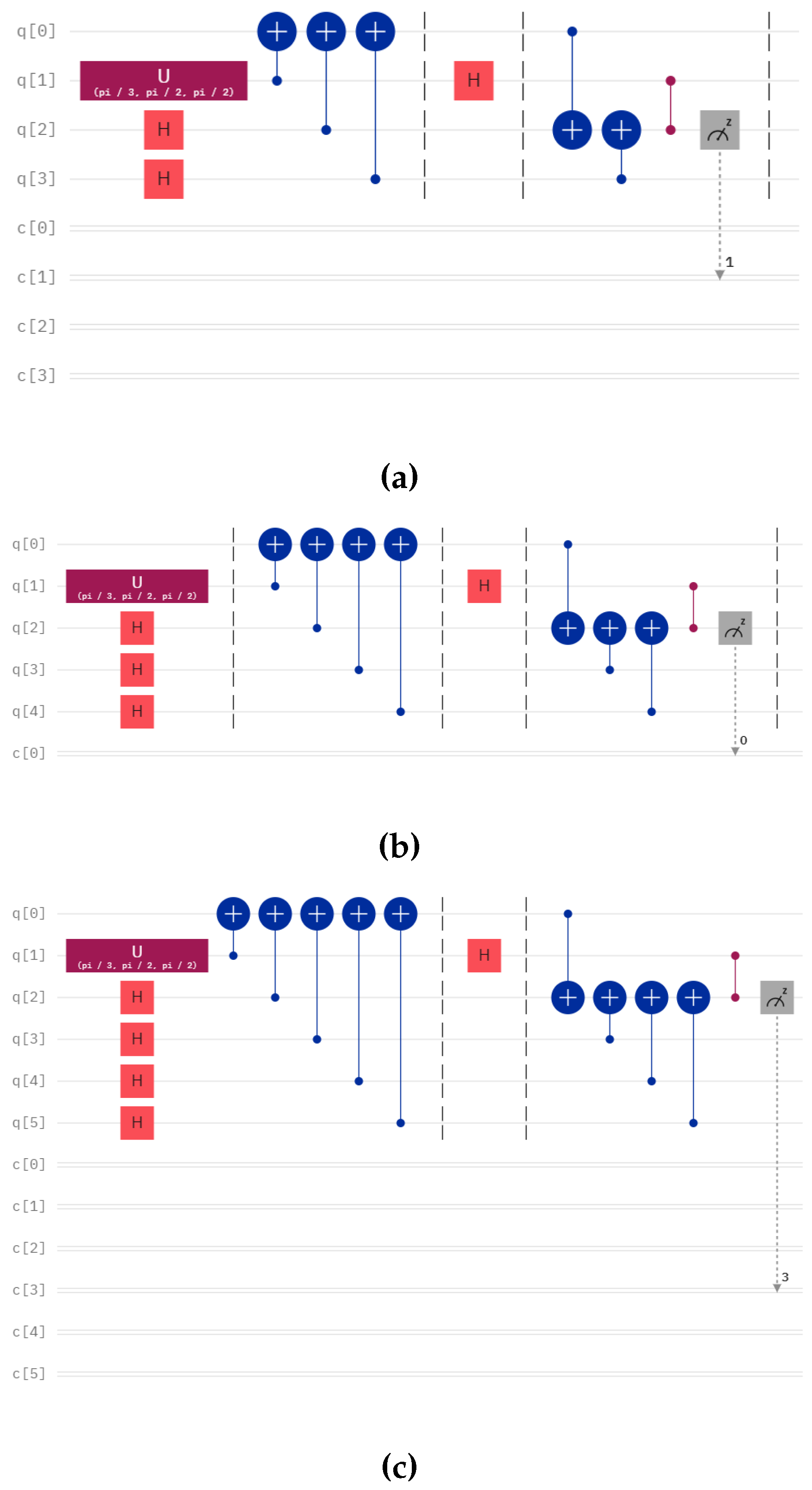
Figure 2. Circuit for teleporting qubits from eight-dimensional coin space to four-dimensional with one controller.

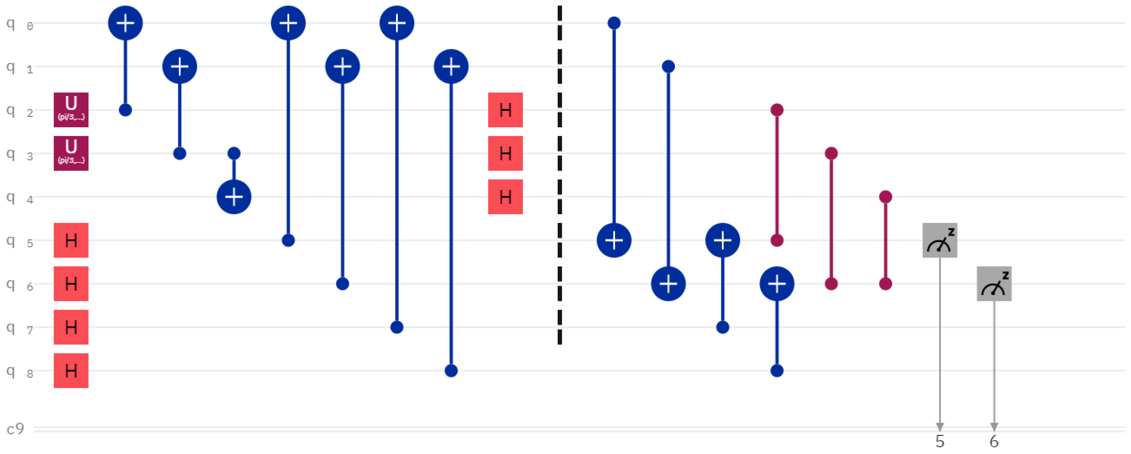
Table 1. This table contains the output of one qubit teleportation for different numbers of controllers in the IBM QASM Simulator of IBM.

Controllers	Theoretical	$\| 0 〉$	$\| 1 〉$
1	$\frac{\sqrt{3}}{2} \| 0 〉 + \frac{ι}{2} \| 1 〉$	0.76	0.24
2	$\frac{\sqrt{3}}{2} \| 0 〉 + \frac{ι}{2} \| 1 〉$	0.75	0.25
3	$\frac{\sqrt{3}}{2} \| 0 〉 + \frac{ι}{2} \| 1 〉$	0.74	0.26

Table 2. This table contains the output of two-qubit teleportation for different numbers of controllers in the IBM QASM Simulator of IBM.

Controllers	Theoretical	$\| 0 〉$	$\| 1 〉$
1	$\frac{\sqrt{3}}{2} \| 00 〉 + \frac{ι}{2} \| 11 〉$	0.74	0.26
2	$\frac{\sqrt{3}}{2} \| 00 〉 + \frac{ι}{2} \| 11 〉$	0.75	0.25
3	$\frac{\sqrt{3}}{2} \| 00 〉 + \frac{ι}{2} \| 11 〉$	0.74	0.26

Table 3. This table contains the output of three-qubit teleportation for different numbers of controllers in the IBM QASM Simulator of IBM.

Controllers	Theoretical	$\| 0 〉$	$\| 1 〉$
1	$\frac{\sqrt{3}}{2} \| 00 〉 + \frac{ι}{2} \| 11 〉$	0.75	0.25
2	$\frac{\sqrt{3}}{2} \| 00 〉 + \frac{ι}{2} \| 11 〉$	0.74	0.26
3	$\frac{\sqrt{3}}{2} \| 00 〉 + \frac{ι}{2} \| 11 〉$	0.75	0.25

Disclaimer/Publisher’s Note: The statements, opinions and data contained in all publications are solely those of the individual author(s) and contributor(s) and not of MDPI and/or the editor(s). MDPI and/or the editor(s) disclaim responsibility for any injury to people or property resulting from any ideas, methods, instructions or products referred to in the content.

© 2024 by the authors. Licensee MDPI, Basel, Switzerland. This article is an open access article distributed under the terms and conditions of the Creative Commons Attribution (CC BY) license (http://creativecommons.org/licenses/by/4.0/).

Copyright: This open access article is published under a Creative Commons CC BY 4.0 license, which permit the free download, distribution, and reuse, provided that the author and preprint are cited in any reuse.

Downloads

232

Views

Comments

Subscription

Notify me about updates to this article or when a peer-reviewed version is published.

MDPI Initiatives

Important Links

Choose an area of interest and we will send you notifications of new preprints at your preferred frequency.

Disclaimer

Controlled Quantum Communication Using Quantum Random Walk

Abstract

Keywords:

Subject:

1. Introduction

1.1. Quantum Communication

1.2. Quantum Random Walk

1.3. Weak Measurements

1.4. Contributions of the Paper

1.5. Organization

2. Related Works

3. Theory

3.1. Quantum Random Walk

3.2. Theoretical Framework of the Algorithm

3.3. Receiver Operation

3.4. Communication between Symmetrical and Asymmetrical Coin space

3.5. Amplitude Damping

3.6. Weak Measurement Based Protection Protocol

3.7. Quantum State Tomography

3.8. Quantum Fidelity

3.9. Attack Analysis

4. Experimental Results

4.1. Circuits Output on Simulators

4.2. Results of Quantum State Tomography

4.3. Results of Weak Measurements

5. Discussion and Conclusion

Acknowledgments

Appendix

References

MDPI Initiatives

Important Links

Subscribe