Origin of the Dark Energy

1. INTRODUCTION

We are going to begin by describing the Dirac delta function, to explain the concept of a zero-phase non-causal system and compare it with a minimum-phase causal system.

As a practical example, to demonstrate the existence of dark energy, we are going to use a test that is used in terrestrial seismic with vibroseis, gas and oil exploration, called Hardwire Similarity.

1.1. Theoretical analysis of the Dirac delta function (Impulse) and its analogy with the Big Bang

The collision of two stellar black holes with an average mass of 40 solar masses, detected by the LIGO and Virgo observatory, confirmed the existence of gravitational waves.

Now, if we take this to the Big Bang, to the inflationary period, the immense energy released would be expected to generate a spectrum of gravitational waves; This affirmation is very important and based on this we are going to work.

Let us define the impulse function &(t) or also called the Dirac delta function.

&(t) = {∞, t = 0 ^ 0, t ≠ 0}

Graphical representation of the impulse function:

Figure 1. Impulse function.

Figure 1. Impulse function.

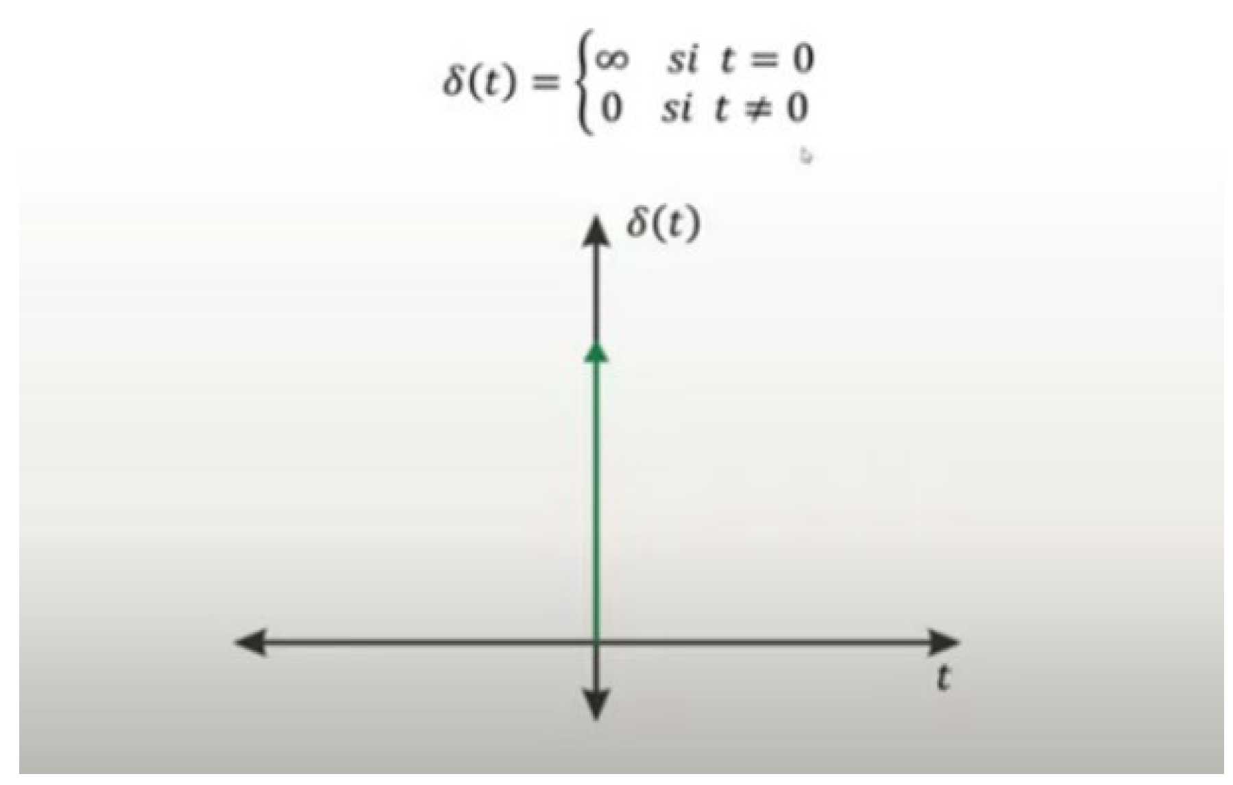
We see that for t = 0 the value of the impulse function tends to infinity (In some literature for t = 0, the Dirac delta function has a generic unitary amplitude) and that for t ≠ 0 the value is 0. Based on what has been said, we can make an analogy with the expansion of the Big Bang and say that at time t = 0, its expansion would behave like a pulse of infinite energy.

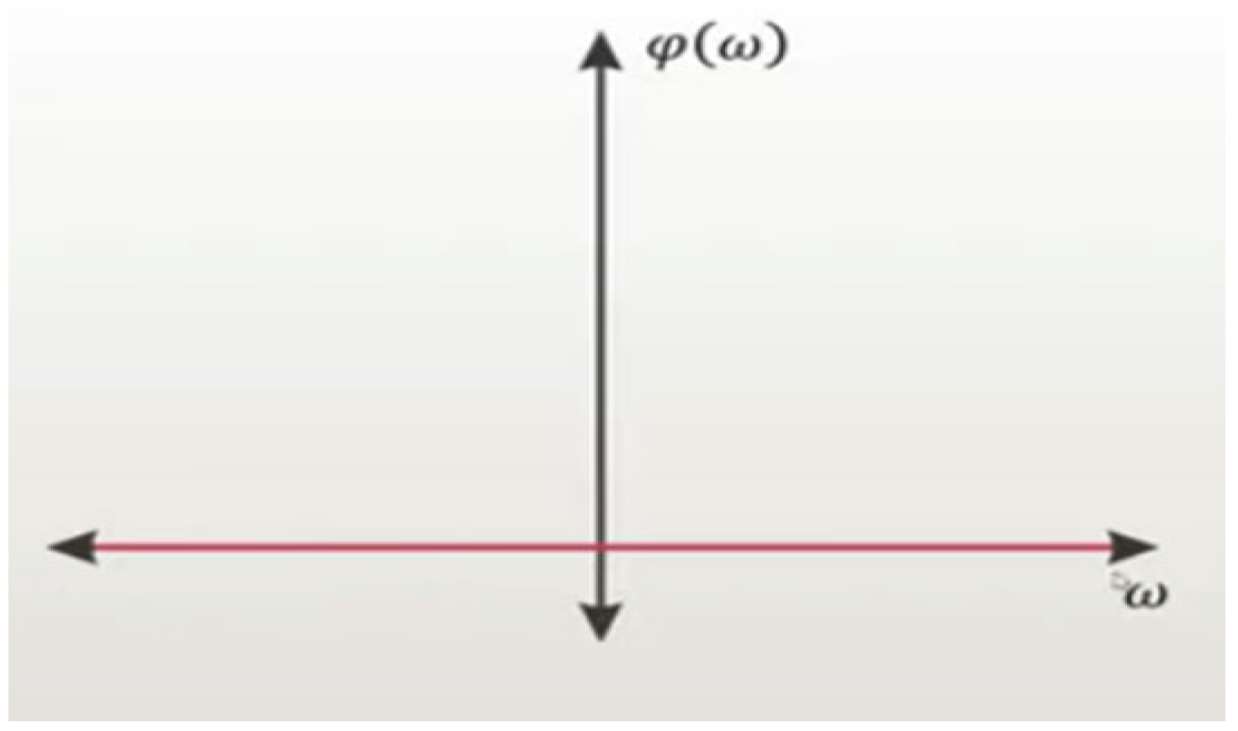
If we analyse the amplitude and phase spectrum of the Fourier transform of the impulse function, we see that the amplitude spectrum is equal to a constant K for all frequencies and the phase spectrum is equal to 0 for all frequencies.

Again, making an analogy between the impulse and the burst of energy of the Big Bang released at time t = 0, we can say that for all frequencies the amplitude spectrum is constant and the phase spectrum is zero.

Figure 2. Amplitude spectrum of the function &(t) in the frequency domain.

Figure 2. Amplitude spectrum of the function &(t) in the frequency domain.

Figure 3. phase spectrum of the function &(t) in the frequency domain.

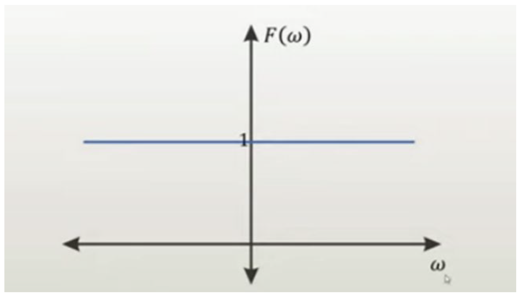
Figure 3. phase spectrum of the function &(t) in the frequency domain.

Let's try to clarify what has been explained and let's say that at t = 0, at the moment of the Big Bang explosion, the enormous amount of energy released generates infinite waves of energy (infinite frequency spectrum) that will propagate through space in all directions, each wave with the same amplitude and the same phase.

For the amplitude spectrum to be constant and the phase spectrum to be zero, we will infer that it is a zero-phase system.

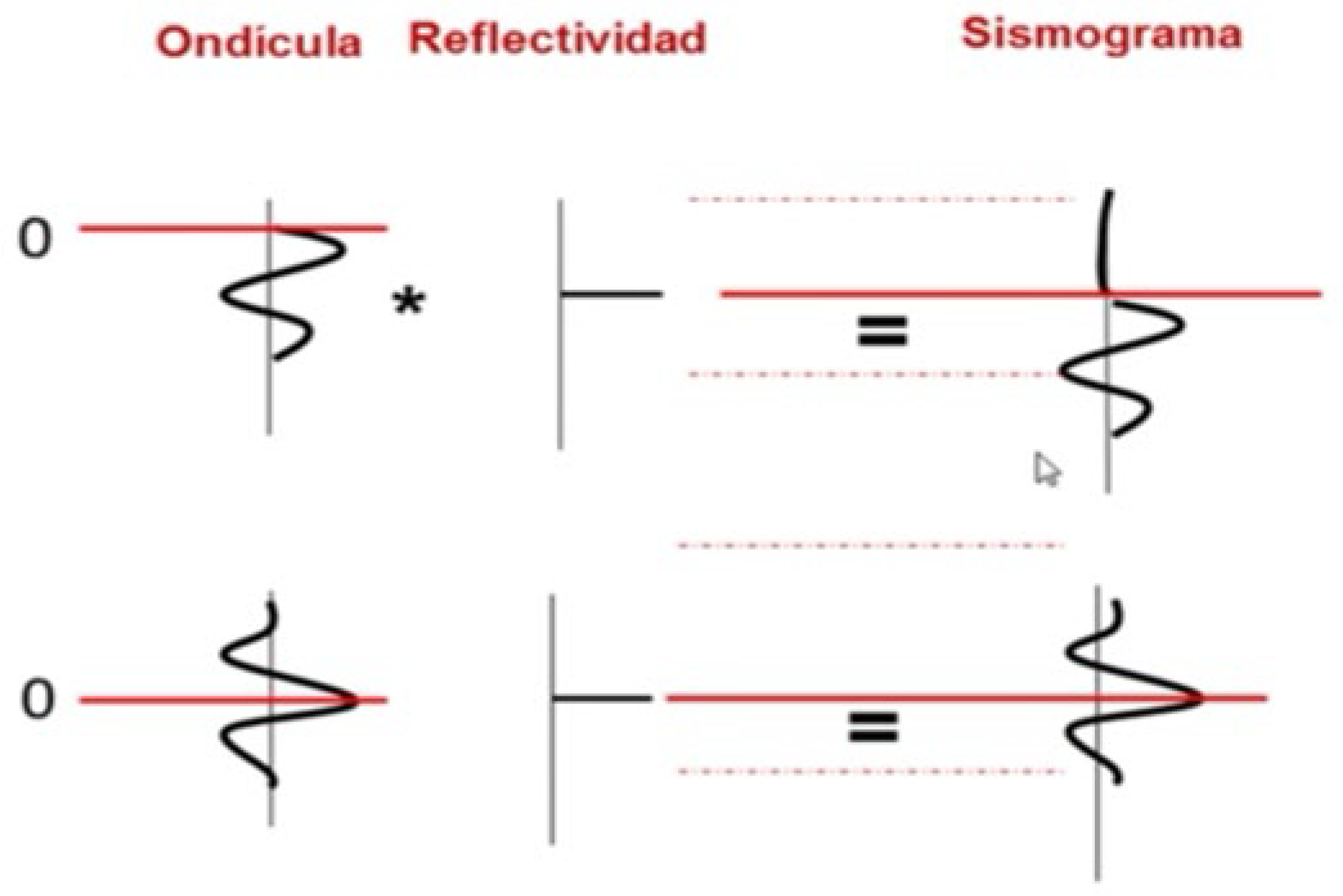
We will introduce the concept of convolution and for this we will make the following analogy. When we do seismic exploration studies to look for gas or oil and use dynamite as a source of energy, the signal that we pick up on our seismic sensors is the result of the energy released by exploding the dynamite that mixes or convolves with the physical characteristics of the earth. If we analyse the signals captured by geophones in the frequency domain, we see that the amplitude and phase spectra depend on the physical characteristics of the earth. We are dealing with a causal type minimal phase system.

According to the above, we can say that the energy released and produced by the Big Bang mixes or convolves with the physical characteristics of the existing universe to produce infinite waves of energy that propagate through space-time (gravitational wave spectrum), whose spectrum of amplitude and phase in the frequency domain, will depend on the physical characteristics of space-time at the moment of the explosion in analogy with the physical characteristics of the Earth. In other words, we can consider the Big Bang as a minimum phase causal system.

In the following example, we will show the difference that exists between a zero-phase, non-causal system and a minimal-phase, causal system.

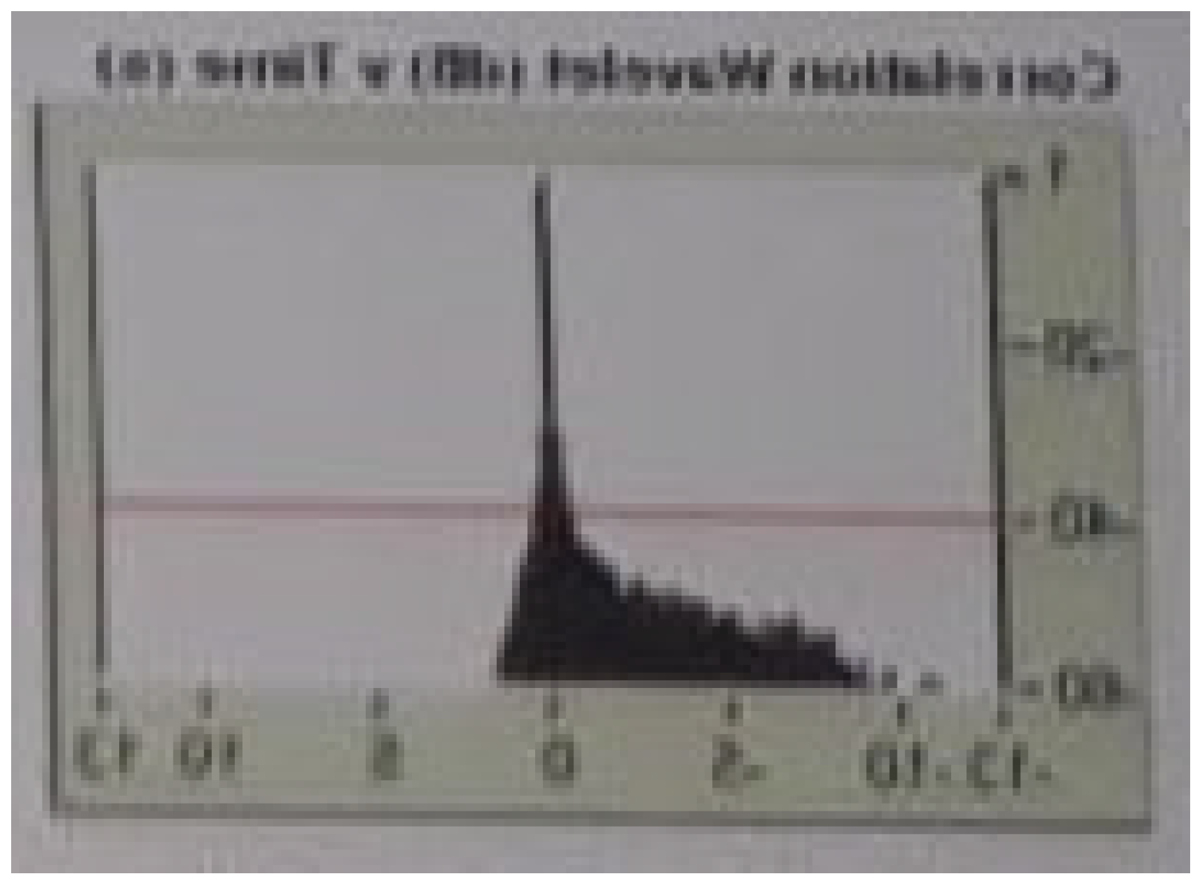
Figure 4. Wavelet with minimum phase in the upper graph and a wavelet with zero phase in the lower graph.

Figure 4. Wavelet with minimum phase in the upper graph and a wavelet with zero phase in the lower graph.

The Lambda-CDM model and the FLRW metric are indicating that the expansion period of the universe, called inflation, behaves as an approximation of the Dirac function for t = 0, the energy released is infinite, spectrum of constant amplitude and spectrum of phase 0.

What would happen if we consider the causal system, minimum phase and anisotropic? that is, that the energy released during inflation is not transmitted instantaneously to space-time and that the expansion of gravitational waves during inflation is a function of time. Possibly these considerations could end or solve the problem of dark energy generated by an incorrect conjecture when considering the isotropic universe, that is, we would be affirming that Einstein's field equations would not be adequate to analyse the evolution of the universe or would eventually be needing of a fine adjustment.

I propose that the space-time expansion of the inflationary era of the Big Bang behaves as a system causal, of minimum phase, in which the released energy is transmitted to space-time with a minimum delay and the propagation of the generated gravitational waves depend of the characteristics of the space-time, physical environment. An example of this behaviour is analogous to the seismic exploration method with explosives, in which the entire system is of minimum phase (causal) and the waves generated by the explosion are transmitted to an anisotropic medium, that is, with different refractive and reflection coefficients.

We are going to highlight the following in this analysis:

1) If we analyse the Dirac delta impulse function, in the frequency domain, the amplitude spectrum tells us that we have infinite frequencies and the zero-phase spectrum tells us that all the energy is transmitted to the medium instantaneously, we are facing a zero-phase, non-causal system.

2) If we analyse the Big Bang as a real system analogous to the explosion of dynamite in seismic prospecting; In the frequency domain, the amplitude spectrum tells us that we have infinite gravitational waves and the phase spectrum tells us that energy is not transmitted instantaneously to space-time, the transmission of energy to space-time is a function of time, we are faced the presence of a minimal phase causal system. It is precisely this characteristic that a minimal phase causal system has, which takes on significant importance in order to explain the origin of dark energy.

2. APPLICATION OF THE MODEL AND RESULTS

2.1. Analysis of the propagation of seismic waves using the Vibroseis method and its analogy with the Big Bang.

Real example:

Figure 5. Plot of seismic channels for file 9013.

Figure 5. Plot of seismic channels for file 9013.

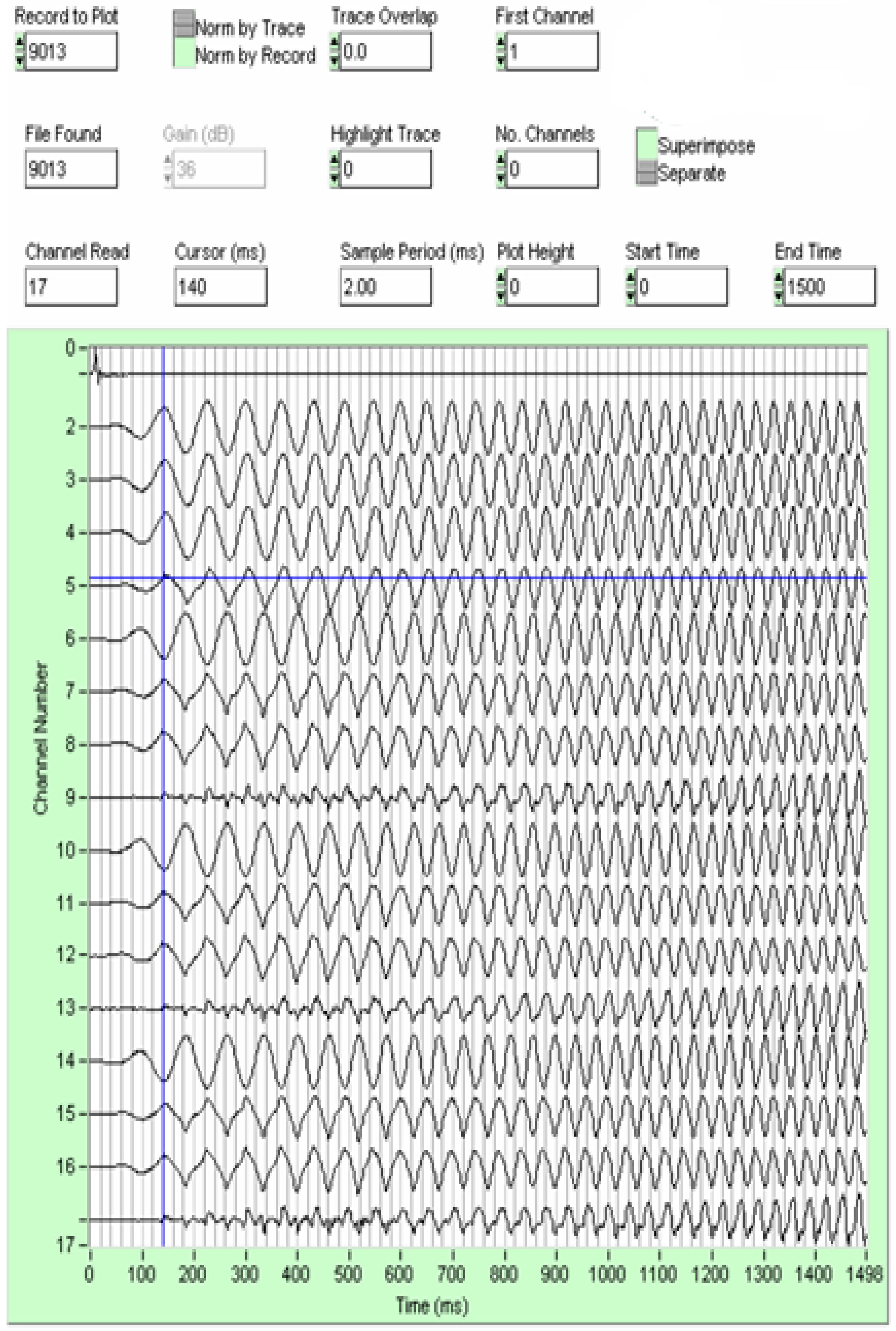
Figure 6. Description of acquisition channels vs File.

Figure 6. Description of acquisition channels vs File.

Figure 7. -Description of the seismic sweep vs File.

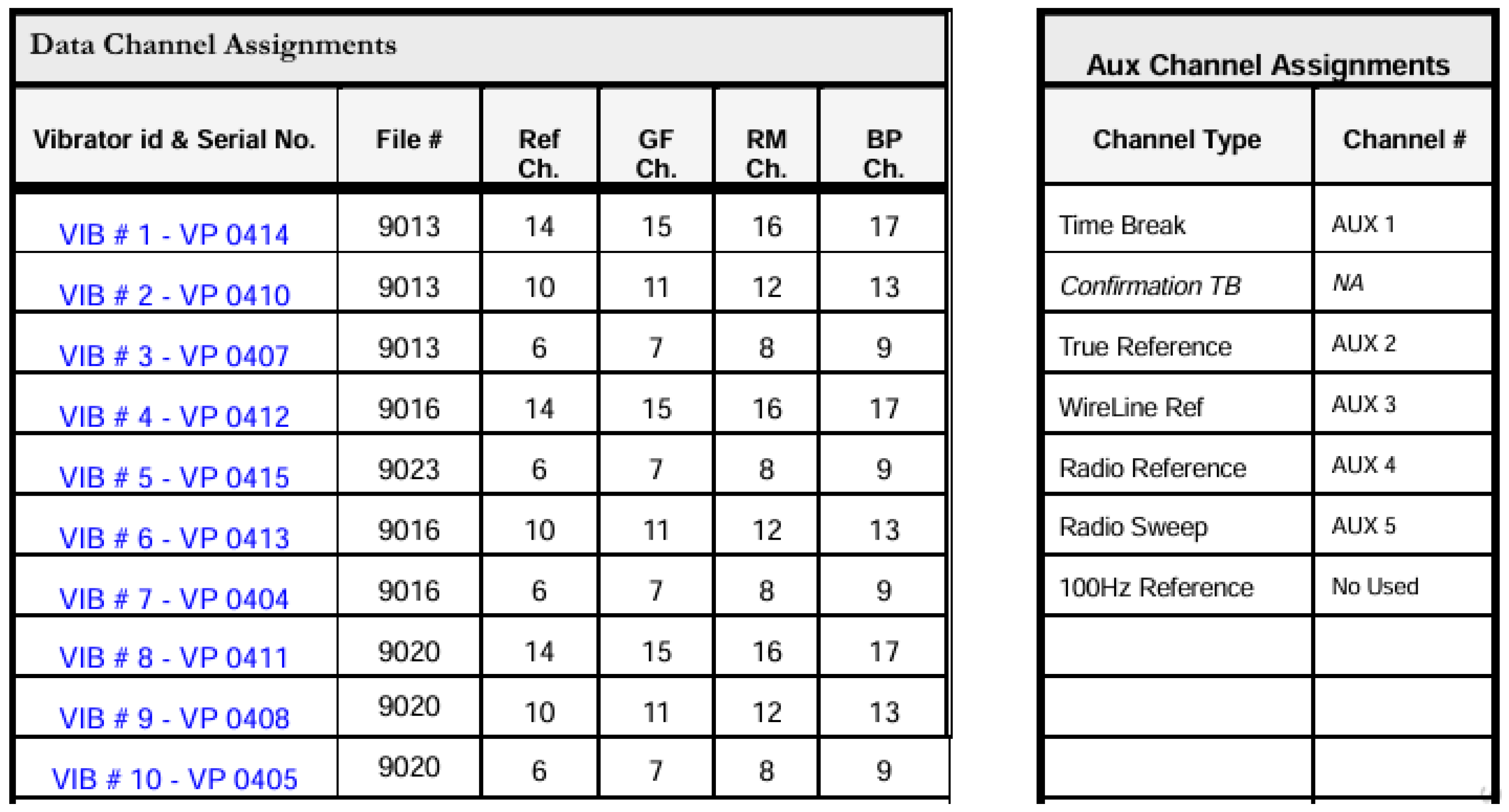
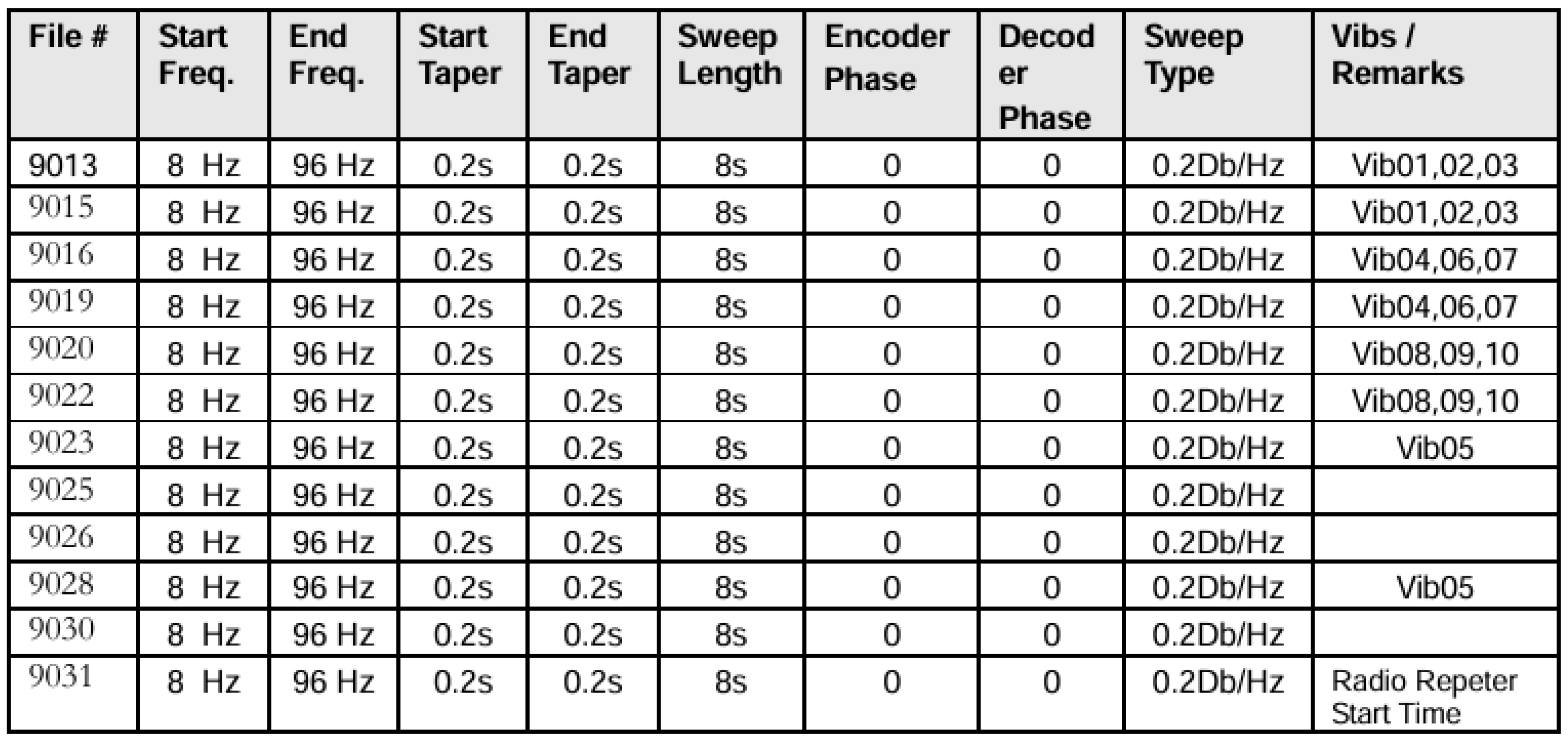
Figure 7. -Description of the seismic sweep vs File.

In our analysis, we are going to use a Hardwire Similarity, Start up.

The Hardwire Similarity is a test carried out in Seismic that uses Vibroseis, to measure the polarity of the Recording system and the polarity of the Vibroseis system as a whole; which must comply with the SEG (Geophysical Exploration Society) standards.

The Hardwire Similarity also serves to measure the start time or zero adjustment, that is, the synchronization of the system.

Figure 5, shows the graph of the signals recorded on tape, which we used to process the tests.

In Figure 6, the signals are described per channel; the graph on the right describes what each signal is in the first 5 channels, from the graph in Figure 5.

On the left, it is described what each signal is, from channel 6 to channel 17, from the graph in Figure 5.

Figure 7, describes the sweep used in the test vs File. It tells us that its frequency ranges from 8 Hz to 96 Hz, that the sweep time is 8 s and that the sweep type used is 0.2 Db/Hz.

As a general comment, to process the signals we have used a Testif-i key.

Now, using graphs we are going to try to understand the mathematical process of correlation.

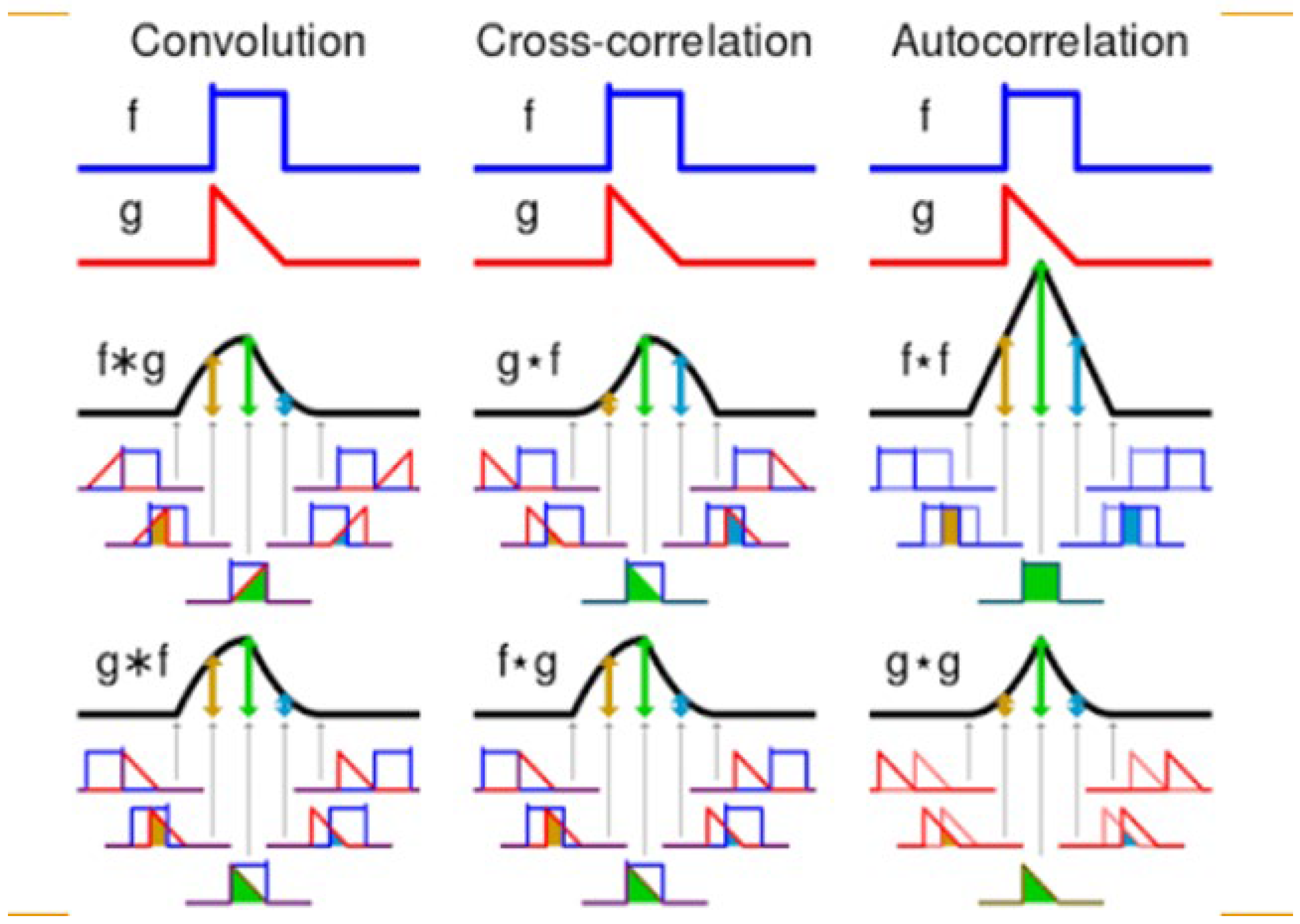
Figure 8. Graphic explanation of the convolution, cross-correlation and autocorrelation process.

Figure 8. Graphic explanation of the convolution, cross-correlation and autocorrelation process.

To begin our signal analysis, it is necessary to explain the following:

Vibroseis: It is a truck that consists of a servomechanism system that is divided into two parts; an electrical part, which generates the ideal electronic sweep. A mechanical part, which is responsible for transforming the electrical sweep into a mechanical sweep, which is applied to the ground. In our work we use 60,000 Lb Vibroseis.

Casa Blanca: It is the Recording truck, when the vibroseis executes the seismic sweep, this signal is transmitted to the different layers of the earth, is reflected in the different interfaces and returns to the surface, where it is captured by the geophones. This signal is transported from the geophones to recording truck, where it is processed (correlated) and recorded on tape.

Spread: It is the set of geophones, cables and boxes that are connected to the recording truck, which are distributed on the ground, used to capture the seismic signals emitted by the vibroseis.

Now we are going to analyze the following signals:

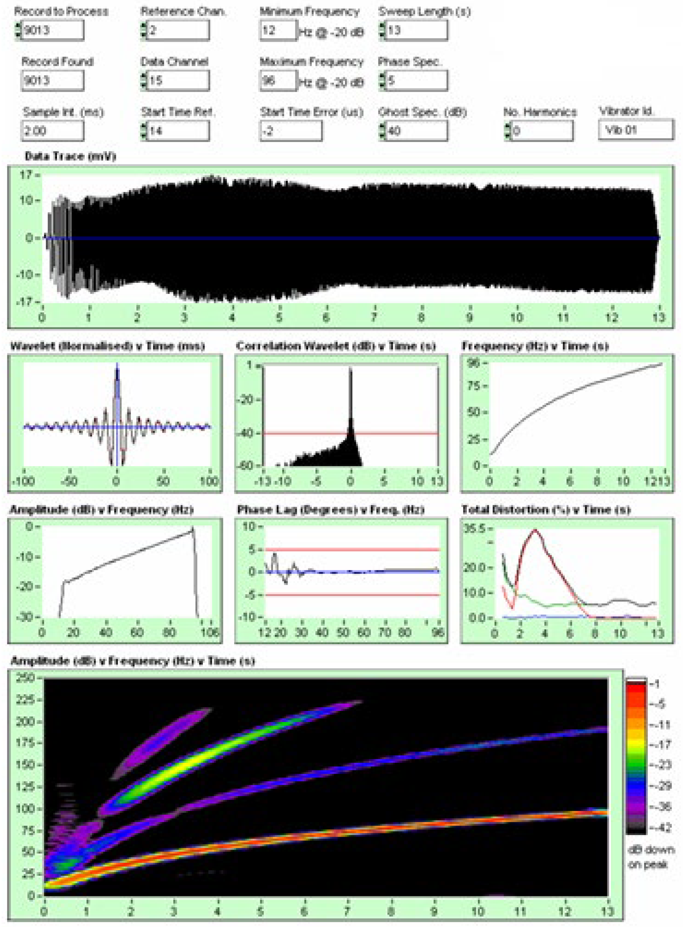
Figure 9. Analysis of channel (2, 2), True Reference signal (see Figure 5).

Figure 9. Analysis of channel (2, 2), True Reference signal (see Figure 5).

From the processing of this signal we are going to rescue the following image:

Figure 10. - Envelope of autocorrelation canal (2,2).

Figure 10. - Envelope of autocorrelation canal (2,2).

It is important to highlight that this signal is symmetrical on both sides, has no noise and reaches up to -120 dB common mode rejection of the signal/noise , It is a pure electronic signal.

Now we are going to analyze the following signal:

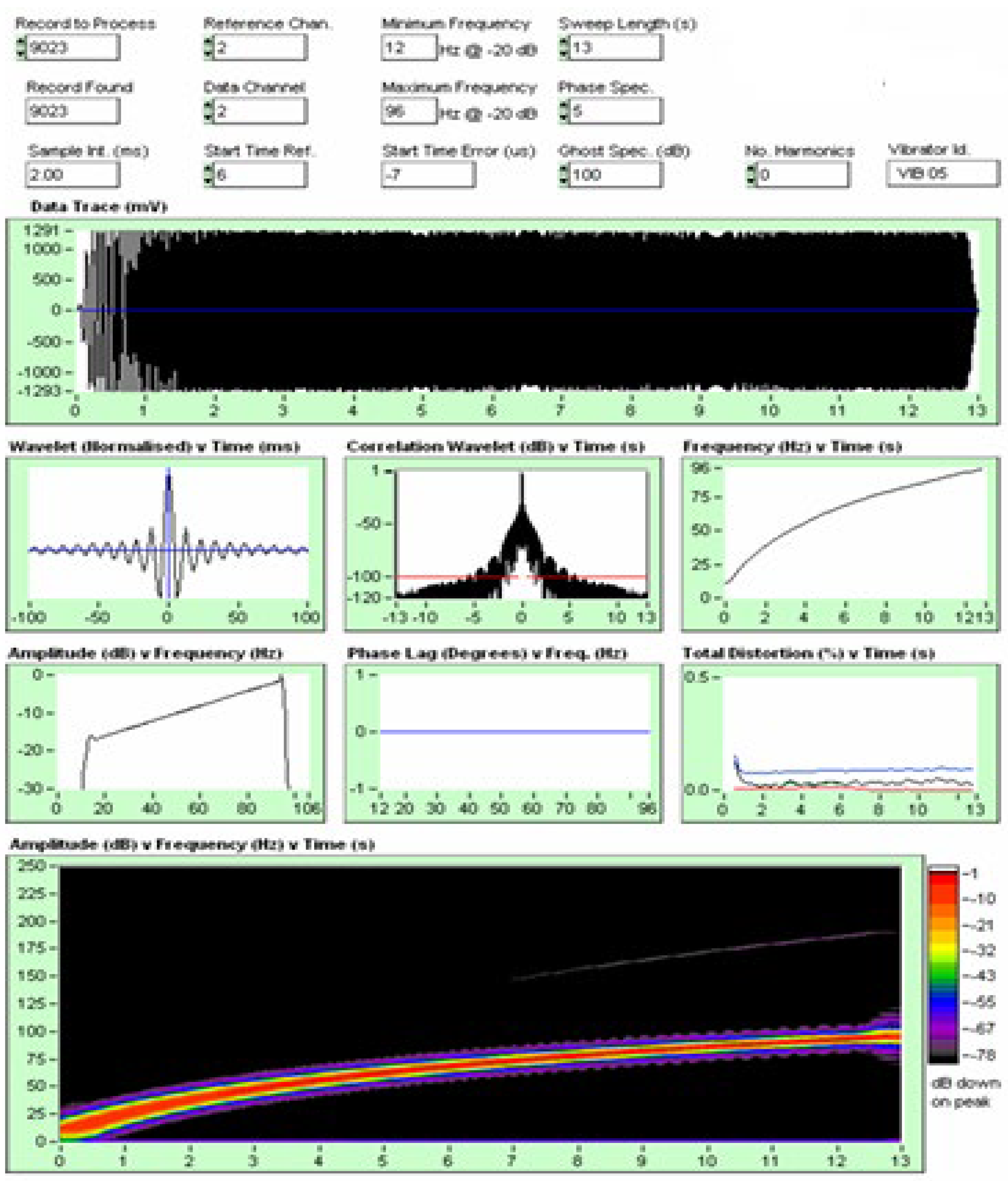
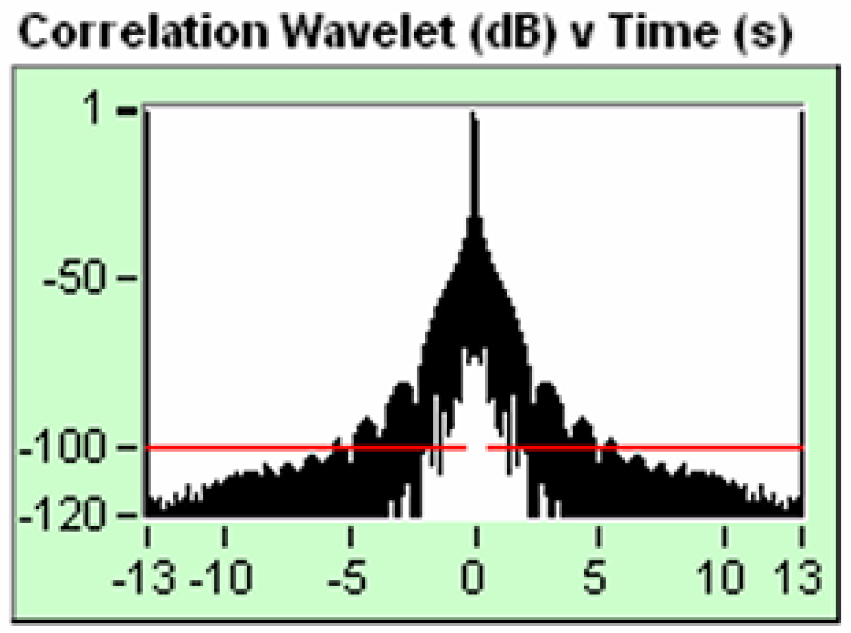
Figure 11. Analysis of channel (2, 15), True Reference signal vs - Ground Force (see Figure 5).

Figure 11. Analysis of channel (2, 15), True Reference signal vs - Ground Force (see Figure 5).

It is important to note that we are analyzing the signal from channel 2, true reference (it is a pure electronic signal) and the signal from channel 15, - ground force (It is the signal that the accelerometers of the Vibrosis truck capture, they are processed and sent to the recording truck, which are recorded on tape and displayed on the monitor, see Figure 5).

From the processing of this signal we are going to rescue the following image:

Figure 12. Envelope of cross-correlation canal (2,15).

Figure 12. Envelope of cross-correlation canal (2,15).

Figure 13. Envelope of cross-correlation canal (15,2), mirror image.

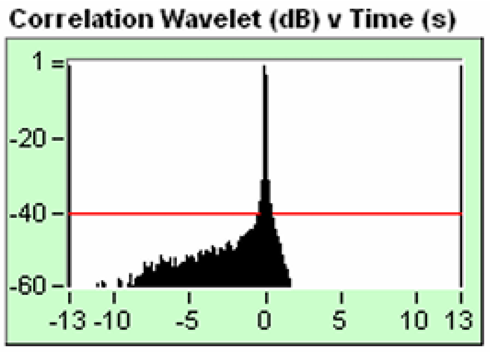
Figure 13. Envelope of cross-correlation canal (15,2), mirror image.

Let's first analyze image 12 and 13.

If we analyze Figure 8, we see that it is not the same to cross correlate the channels (2, 15) or cross-correlate the channels (15, 2), from now on, we are going to use Figure 13, the envelope of cross correlation of the channels (15, 2) for the simple reason that in this picture the noise corresponds to the right of zero, that is, for positive time, this is the main reason why we use this envelope of cross-correlation configuration. In Figure 12, the signal/noise is to the left of zero, for negative times and that confuses our interpretation.

The correct thing would be to use the Testif-i key to process the signal again, perform the envelope of cross-correlation of the signals (15, 2) and obtain the correct image, unfortunately I do not have that Testif-i key; for which I am forced to use the mirror image and give a good explanation.

Now we are going to analyze how everything explained is related to the Big Bang.

To do this, we are going to analyze Figure 10 and Figure 13.

If we analyze Figure 10, it shows the autocorrelation envelope of the signal that corresponds to channel 2 (True Reference, pure electronic signal), it is a symmetrical signal and reaches up to -120 db common mode rejection of the Signal/noise, It has no noise and we can see this in the FK filter that we show below.

Figure 14. Shows the frequency content, FK filter of the channel 2 signal (True Reference).

Figure 14. Shows the frequency content, FK filter of the channel 2 signal (True Reference).

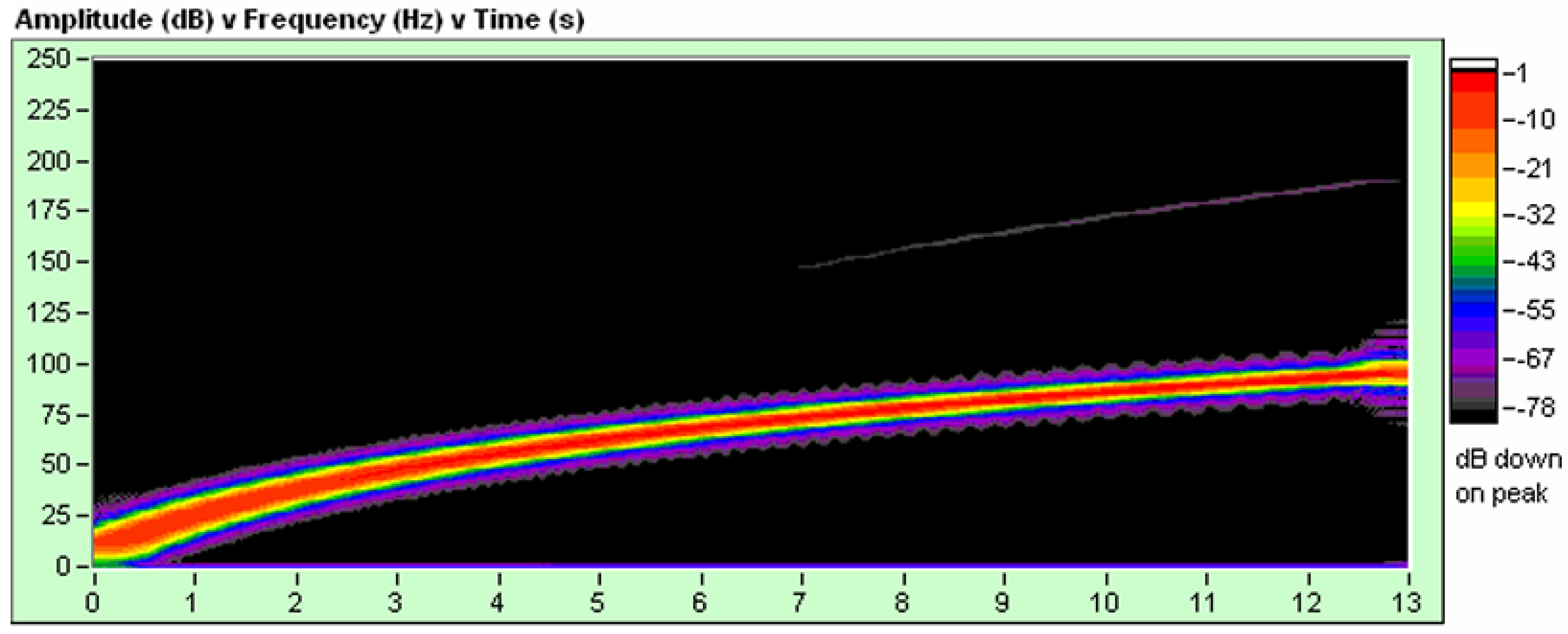
Figure 14, shows the frequency content of the electronic sweep of channel 2 (True Reference), we see that it does not have even or odd harmonics and we do not see noise in the signal, in other words it is a pure, perfect electronic sweep.

This pure electronic signal that corresponds to channel 2 (True Reference) is the perfect analogy with the Big Bang. The theory developed to explain the Big Bang, the Lambda-CDM model (metrica FLRW), analyzes the Big Bang as if the expansion were of a single fundamental frequency, this makes us think that the expansion should have a single Hubble constant. This expansion does not consider even and odd harmonic frequencies or noise in the signal, which is very important because these additional energy contributions make the Hubble´s constant variable and most importantly, the additional energy makes the expansion of the universe accelerate.

If we analyze figure 13, it shows the envelope of the autocorrelation of the signal that corresponds to the channel (15, 2) that corresponds to the signal -Ground Force vs True Reference, it is an antisymmetric signal and we observe that from - 40 db common mode rejection of the signal/noise, there is a noise content and we can see this in the FK filter shown below.

Figure 15. - Shows the frequency content, FK filter of the channel 15, signal (-Ground Force).

Figure 15. - Shows the frequency content, FK filter of the channel 15, signal (-Ground Force).

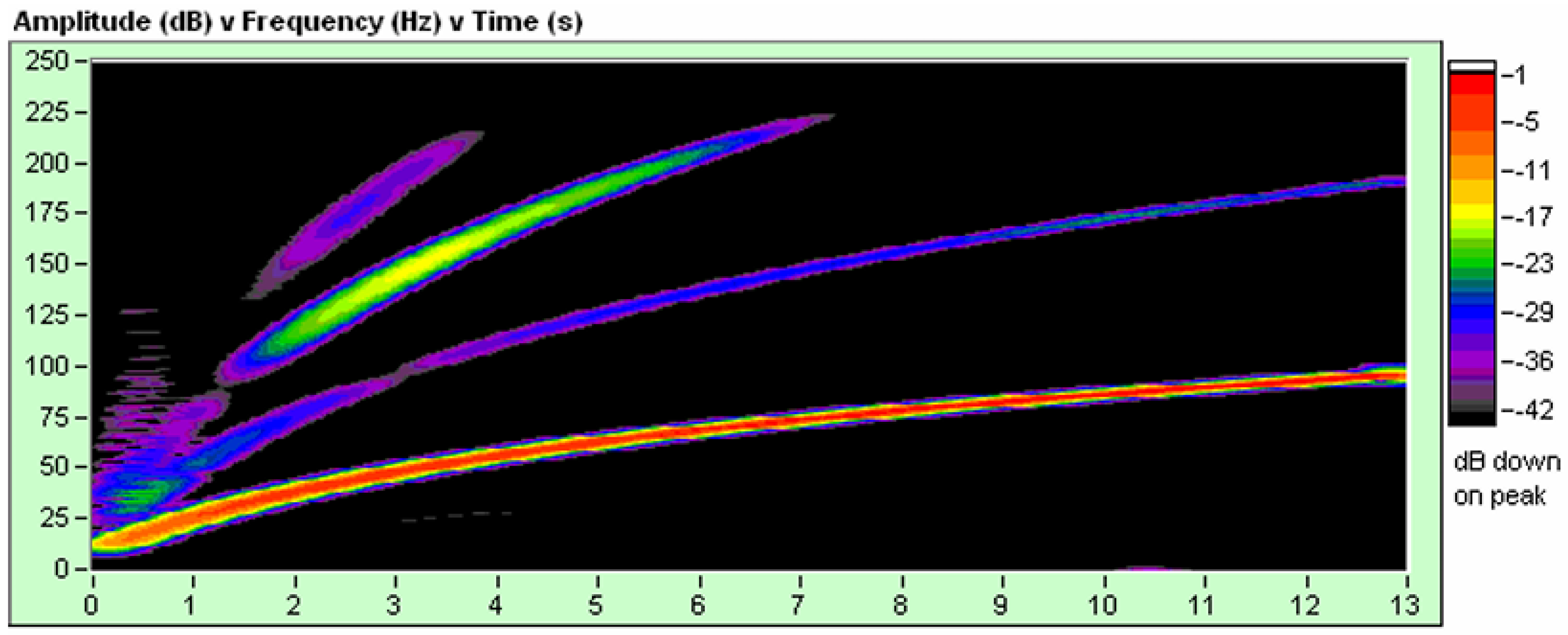
If we make an analogy with the Big Bang, in addition to the fundamental frequency, we must consider the harmonics and inherent noise to be able to correctly interpret the expansion of the universe.

Now we are going to analyze it from another point of view, to understand the origin of dark energy.

Let's analyze the distortion graph, from figure 9, we rescue the following graph :

Figure 16. Total distortion % vs Time (s).

Figure 16. Total distortion % vs Time (s).

Remember that figure 9 represents a pure sweep signal without distortion. If we look at Figure 16, we see that the distortion is approximately of the order of 0.1%. We can also see this in figure 14, FK filter, in which it is observed that there is no dostortion.

If we make an analogy with the Big Bang, the expansion of space-time, we can consider the example of the balloon that inflates, it does so with a fundamental frequency, there is no distortion, noise, it is an ideal expansion that follows the FRWL metric, the equations of general relativity and all the theoretical development framed in the theory of modern Cosmology.

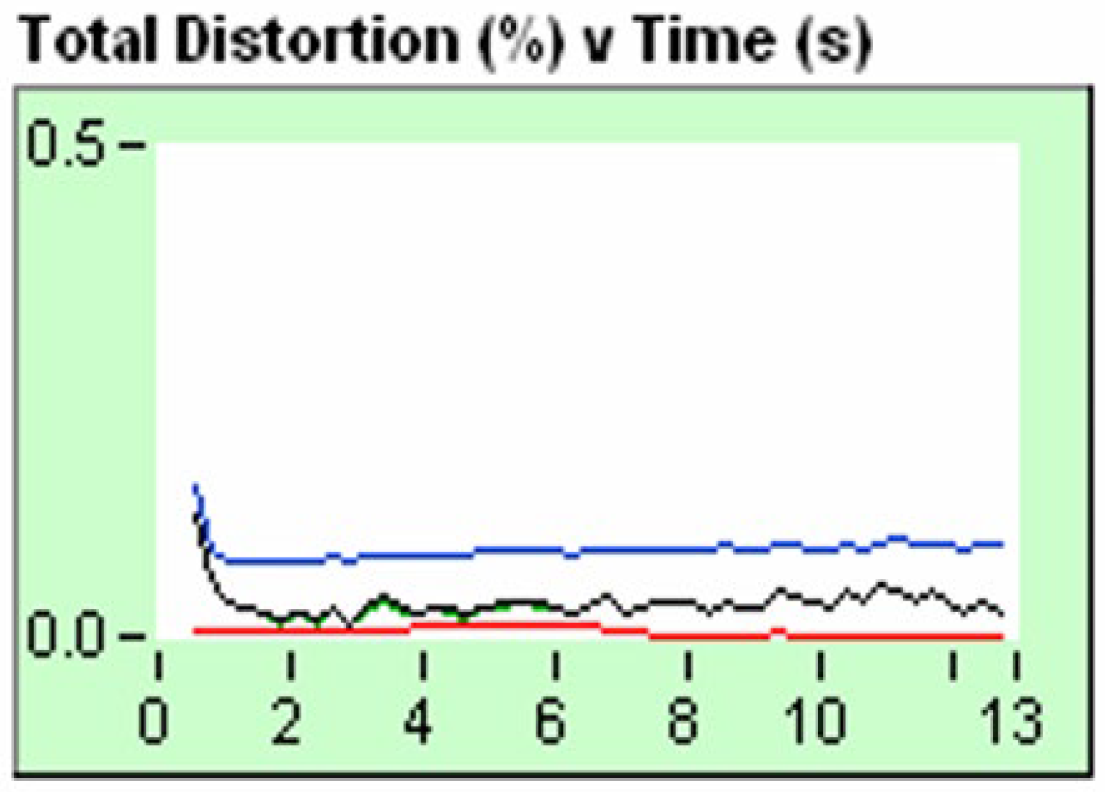
Let's analyze the distortion graph, from figure 11, we rescue the following graph :

Figure 17. Total distortion % vs Time (s).

Figure 17. Total distortion % vs Time (s).

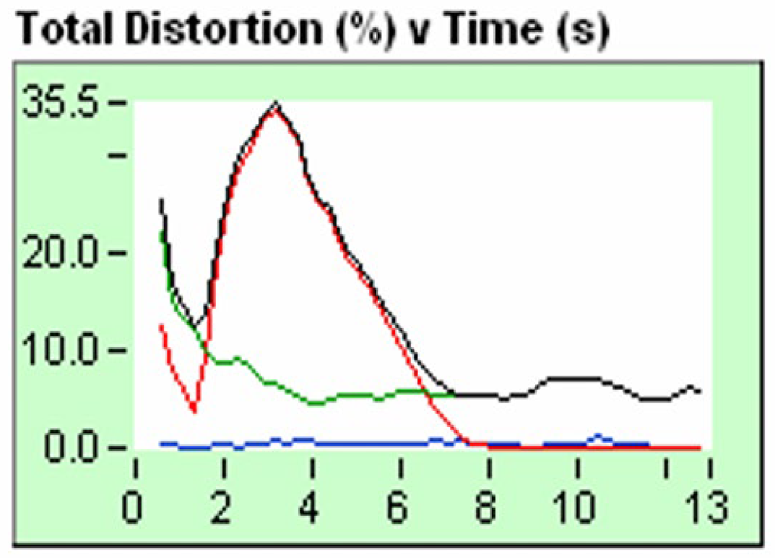
In figure 17, we are analyzing the distortion graph of a real signal, it is a signal emitted by the vibroseis truck that interacts with the terrain. We see that the distortion peak is approximately 35%. That distortion is produced by even harmonics, odd harmonics and additional noise. We can also see this in figure 15, FK filter, in which the frequencies of even, odd harmonics and additional noise are observed.

Again, if we make an analogy with the Big Bang, it is important to understand the following concept. The expansion of space-time produced by the Big Bang, in addition to producing a frequency spectrum of gravitational waves, produces an additional spectrum of even and odd harmonics, additional noise that is the result of the convolution of the gravitational wave spectrum produced by the Big Bang with space-time being the medium through which gravitational waves propagate.

The sum of additional energy due to the frequency of even and odd harmonics and additional noise is dark energy. Since this energy distribution is not constant as a function of time, it generates what we call Hubble´s tension, which is nothing more than considering the Hubble´s constant variable.

In general, when the vibroseis truck carries out the sweep, depending on the type of terrain, a distortion of the order of 20% to 50% is produced, when the terrain is volcanic rock the distortion goes up to 80%, also on occasions the distortion exceeds 100% producing a decoupling of the vibroseis truck from the ground, in this situation the force exerted by the earth on the vibroseis truck is greater than the weight of the vibroseis, causing it to make sudden jumps.

Recall that we have hypothesized that the Big Bang behaves as a minimal phase causal system, in other words, the energy contribution is a function of time.

This is how we can correctly understand the following graph:

Figure 18. Supernova Hubble Diagram.

Figure 18. Supernova Hubble Diagram.

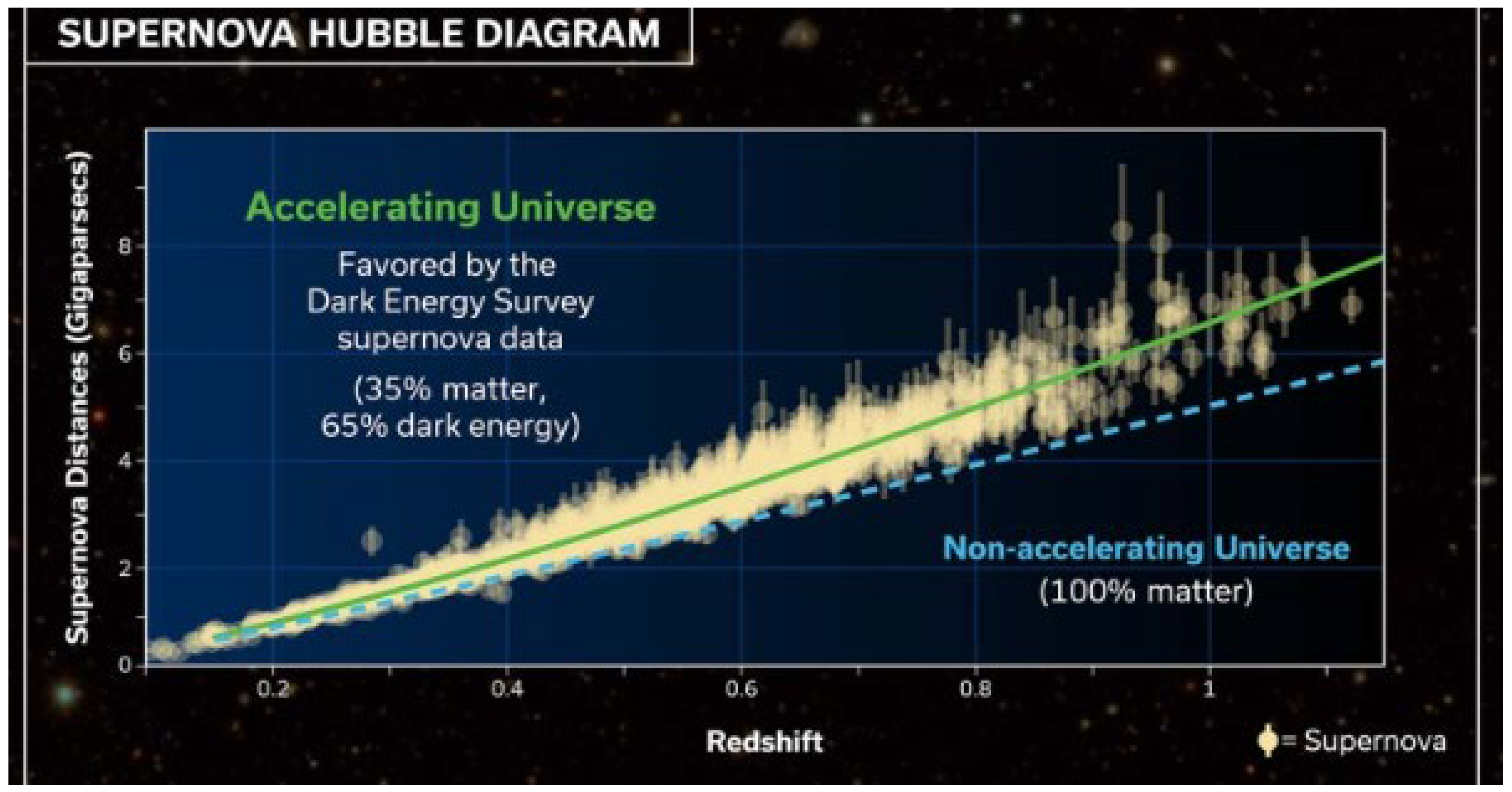
The difference that exists between the dotted light blue line, which corresponds to the non-accelerated universe, and the green line, which corresponds to the accelerated universe, is simply that we are not considering the energy contributions that correspond to the harmonics of the fundamental frequency and the noise inherent, as was analyzed for the example of Hardwire Similarity that is carried out in seismic prospecting. If we consider the contributions of additional energies to the fundamental frequency (harmonics of the fundamental frequency and the noise inherent) as a function of time, we will understand why the expansion of the universe is accelerated and deduce that the Hubble´s constant must be variable.

In Figure 13, we can see that additional energy contribution corresponding to the harmonics and noise in the signal, we can see how from time t = 1 to t = 13 sec; The additional energy decreases from -40 dB to -60 dB common mode rejection of the signal/noise. In Figure 10, which corresponds to a pure electronic signal, we can see that this additional energy does not exist precisely because the signal does not have harmonics and noise. In this case, if we observe for t = 13 s, we see that the signal takes the value of - 120 Db common mode rejection of the signal/noise

Continuing with the analogies of our example, just as we consider that the area in which the seismic survey is carried out exists, it is the physical space which we are going to study to find out if there is gas or oil, this leads us to an important conclusion; when the Big Bang occurred, space-time already existed, in this case we could consider a local big bang in an infinite space-time full of big bang or multiverses.

3. Conclusions

We have demonstrated, through a real example, how the dark energy that we observe in our universe originates.

Figure 19. Dark Energy.

Figure 19. Dark Energy.

We can interpret figure 19 in the following way, if we consider that the expansion of the universe after the Big Bang is carried out with a single frequency, fundamental frequency, we obtain the light Blue dotted line. Now, if we consider that the expansion of the universe after the Big Bang behaves as a causal system of minimum phase and produces a frequency spectrum of gravitational waves, of which the energy contribution of these gravitational waves is a function of time, then we obtain the green Line. This additional energy that is added to the fundamental energy, in addition to generating dark energy, produces the Hubble tension, that is, it makes the Hubble constant variable.

We have explained and demonstrated why the expansion of the universe is accelerated and why the Hubble constant is variable with time.

About the author

HECTOR GERARDO FLORES (ARGENTINA, 1971). I studied Electrical Engineering with an electronic orientation at UNT (Argentina); I worked and continue to work in oil companies looking for gas and oil for more than 25 years, as a maintenance engineer for seismic equipment in companies such as Western Atlas, Baker Hughes, Schlumberger, Geokinetics, etc.

Since 2010, I study theoretical physics in a self-taught way.

In the years 2020 and 2021, during the pandemic, I participated in the course and watched all the online videos of Cosmology I and Cosmology II taught by the Federal University of Santa Catarina UFSC (graduate level).

MARIA ISABEL GONÇALVEZ DE SOUZA (Brazil, 1983). I studied professor of Portuguese language at the Federal University of Campina Grande and professor of pedagogy at UNOPAR University, later I did postgraduate, specialization. I am currently a qualified teacher and I work for the São Joao do Rio do Peixe Prefecture, Paraiba. I am Hector's wife and my studies served to collaborate in the formatting of his articles, corrections, etc; basically, help in the administrative part with a small emphasis in the technical part analyzing and sharing ideas.

HARSHIT JAIN (India, 2008) I was born on July 14, 2008, into a loving family. My father, Ajitendra Kumar Jain, and my mother, Preeti Jain, have been incredibly supportive throughout my life and education. I grew up in Lalitpur, where I attended Jawahar Navodaya Vidyalaya (JNV) for my high school education.

My passion for learning has always driven me toward subjects that explore the mysteries of the universe. I have a particular interest in physics, biology, cosmology, and mathematics. This interest led me to the Pacific Institute of Cosmology, where I am currently pursuing advanced studies in these fields.

One of the most significant influences on my academic journey has been Professor Padhi, a renowned scholar who works with several professors who hold the prestigious title of Fellow of the Royal Society (FRS). His mentorship has been invaluable, guiding me through complex concepts and encouraging me to delve deeper into research.

Throughout my studies, I've engaged in various research projects, some of which have challenged conventional thinking and opened new avenues for exploration. These experiences have not only honed my analytical skills but also strengthened my resolve to contribute meaningfully to the scientific community.

In summary, I am Harshit Jain, a young scientist with a passion for discovery. My journey is just beginning, but I'm excited about the endless possibilities that lie ahead. I owe much of my success to my supportive family, dedicated mentors, and the enriching educational environments I've been fortunate to be a part of. I look forward to continuing my research and making meaningful contributions to the fields I hold dear.

References

- Gival Pordeus da Silva Neto. Estimando parâmetros cosmológicos a partir de dados observacionais. Departamento de Física Teórica e Experimental, Universidade Federal do Rio Grande do Norte. file:///C:/Users/Hecto/Downloads/Estimando_parametros_cosmologicos_a_partir_de_dado.pdf.
- Aurelio Carnero Rosell, Director Eusebio Sánchez Álvaro, Madrid, 2011. Determinación de parámetros cosmológicos usando oscilaciones acústicas de bariones en cartografiados fotométricos de galáxias. TESIS DOCTORAL, UNIVERSIDAD COMPLUTENSE DE MADRID. https://eprints.ucm.es/13761/1/T33317.pdf.
- Anderson Luiz Brandão de Souza, Orientador: Pedro Cunha de Holanda. Oscilações Acústica Bariõnicas. TESIS DE MESTRADO, Universidade Estadual de Campinas, Instituto de Física “Gleb Wataghin”, Campinas 2018. https://sites.ifi.unicamp.br/sobreira/files/2018/07/mestrado-tanderson.pdf.
- J.S.Farnes. A Unifying Theory of Dark Energy and Dark Matter: Negative Masses and Matter Creation within a Modified ΛCDM Framework. https://arxiv.org/abs/1712.07962.
- Eisberg Resnick, Física Cuántica.
- Eyvind H. Wichmann. Física cuántica.
- Sears – Zemansky. Física Universitaria con Física Moderna Vol II.
- Iván García Brao. Ecuación de campo de Einstein, Universidad de Murcia, Facultad de Matemáticas. Trabajo de grado año 2018. https://www.um.es/documents/118351/9850492/Garc%C3%ADa+Brao+TF_77837970.pdf/debaa03b-605b-420d-b3ac-85549b6622c0.
- Luis Felipe de Oliveira Guimarães, Orientadora Maria Emilia Xavier Guimarães. Soluciones de buracos negros na relatividade general, Universidad federal Fluminense, Bacherelado em Física. Trabajo de grado 2015. https://app.uff.br/riuff/bitstream/handle/1/5977/Luiz%20Filipe%20Guimaraes.pdf;jsessionid=4EAAF6CB7A4B776D04C9E6E6573D5919?sequence=1.
- Kostas kokkotas, Field Theory.
- James B. Hartle, Gravity and introduction to Einstein´s General Relativity. [CrossRef]
- Charles W. Misner, Kip S. Thorne and Jhon Archibald Wheelher, Gravitation.
- Benito Marcote, Cosmologia Cuantica y creacion del universe.
- Carlos Rovelli, Quantum Gravity.
- Vinicius Miranda Bragança, Singularidades em teorias f(r) da gravitação. http://arcos.if.ufrj.br/teses/mestrado_vinicius_miranda.pdf.
- María José Herrero, Física de Partículas, el acelerador LHC y el bosón de Higgs.
- J. S. Farnes - Received 22 February 2018 / Accepted 20 October 2018. A unifying theory of dark energy and dark matter: Negative masses and matter creation within a modified ΛCDM framework. [CrossRef]
- Bernard Carr, and Florian Kühnel - Annual Review of Nuclear and Particle Science. Primordial Black Holes as Dark Matter: Recent Developments. https://www.annualreviews.org/doi/10.1146/annurev-nucl-050520-125911. [CrossRef]
- Marc Kamionkowski and Adam G. Riess. The Hubble tension and Early Dark Energy. https://arxiv.org/pdf/2211.04492.pdf. [CrossRef]
- Luis Anchordoqui, Carlos Nuñez and Kasper Olsen. Quantum cosmology and AdS/CFT. https://arxiv.org/abs/hep-th/0007064.
- Flores, H. G. (2023). RLC electrical modelling of black hole and early universe. Generalization of Boltzmann's constant in curved spacetime. J Mod Appl Phys. 2023; 6(4):1-6. https://www.pulsus.com/scholarly-articles/rlc-electrical-modelling-of-black-hole-and-early-universe-generalization-of-boltzmanns-constant-in-curved-spacetime.pdf.
Disclaimer/Publisher’s Note: The statements, opinions and data contained in all publications are solely those of the individual author(s) and contributor(s) and not of MDPI and/or the editor(s). MDPI and/or the editor(s) disclaim responsibility for any injury to people or property resulting from any ideas, methods, instructions or products referred to in the content. |
© 2024 by the authors. Licensee MDPI, Basel, Switzerland. This article is an open access article distributed under the terms and conditions of the Creative Commons Attribution (CC BY) license (http://creativecommons.org/licenses/by/4.0/).
Copyright: This open access article is published under a Creative Commons CC BY 4.0 license, which permit the free download, distribution, and reuse, provided that the author and preprint are cited in any reuse.