Submitted:
21 May 2024
Posted:
22 May 2024
You are already at the latest version
Abstract
Cardiovascular disease (CVD) and obesity are prevalent public health concerns with grave implications for morbidity and mortality, necessitating tailored interventions. This research explores the utility of fuzzy c-means clustering paired with principal component analysis (PCA) in detecting at-risk groups and personalizing health strategies for these conditions. Fuzzy c-means clustering allows for the dynamic classification of individuals into groups based on unique risk factors and intervention outcomes, while PCA aids in distilling complex data sets to uncover underlying patterns. The conjoined use of these methods has shown promise in identifying diverse risk profiles and in forecasting intervention success rates. The study acknowledges limitations, including possible biases stemming from data set composition and analytical parameter selection. Future research aims to refine these tools for clinical application. The results support implementing fuzzy c-means clustering and PCA for delineating specific target populations for health interventions, emphasizing careful use of these analytical approaches. Subsequent studies should focus on correlating these techniques with concrete clinical results to enhance public health measures.
Keywords:
Fuzzy C means
; PCA
; machine learning
; obesity
; CVD
Introduction
Cardiovascular disease (CVD) and obesity are two of the leading causes of morbidity and mortality worldwide, with CVD responsible for 17.9 million deaths annually and obesity affecting more than 650 million adults globally [1]. In recent years, there has been a growing focus on identifying patterns and subgroups within large data sets related to these conditions to develop more effective prevention and intervention strategies.
One approach to identifying patterns and subgroups within large data sets is the use of clustering techniques, such as fuzzy c-means clustering. This technique allows for the assignment of data points to multiple clusters, allowing for a more nuanced and flexible classification system. Fuzzy c-means clustering has been widely used in CVD and obesity research to identify subgroups of individuals with differing risk factors or responses to interventions, allowing for tailoring prevention and treatment strategies [2].
In addition to clustering techniques, principal component analysis (PCA) has also been widely used in CVD and obesity research. PCA is a statistical method that is used to reduce the dimensionality of a dataset by identifying patterns and correlations within the data. By identifying these patterns, PCA allows for identifying subgroups within large data sets and tailoring interventions to specific individuals [3].
The fuzzy c-means clustering has been shown to be particularly effective in CVD and obesity research. For example, one study utilizing the technique in CVD research found that the FCM clustering technique was effective in identifying subgroups of individuals with differing levels of cardiovascular risk [4].
To illuminate the intricate relationship between obesity and cardiovascular diseases (CVD), cutting-edge techniques like fuzzy clustering and principal component analysis have been key. These methods are crucial for dividing the obesity condition into specific groups, each with its own cardiovascular risk factors. Numerous studies have utilized these tools to refine the categorization of individuals suffering from both obesity and CVD [5,6].
Moreover, a deep dive into these methods reveals their shortcomings and potential biases when put to use. The research emphasizes the need for strict consideration of data complexity and the solidity of analytical approaches. This critical viewpoint guides upcoming research, bolstering the methodological exactitude necessary for scholarly research [7].
The aim of this study is to identify patterns of obesity in people and analyze the relationship of each pattern with susceptibility to heart disease using Fuzzy C-Means (FCM) Clustering and principal component analysis.
Next, we will launch into an extensive examination of pivotal research that has greatly advanced our knowledge in this field.
Related Work
The integration of Fuzzy C-Means (FCM) Clustering and Principal Component Analysis (PCA) in public health offers a promising machine learning approach to address the burgeoning issues of cardiovascular disease (CVD) and obesity. These data-driven techniques enhance the understanding and management of these complex health challenges.
FCM clustering has been utilized to stratify health-related data effectively, thereby aiding in the understanding of disease patterns and healthcare optimization. [8] demonstrated the application of FCM clustering in grouping healthcare centers based on diarrheal disease, revealing its potential to inform public health improvements. Similarly, [9] discussed the utilization of FCM clustering to manage large healthcare datasets, emphasizing the algorithm's capacity to provide insights by classifying data points based on similarity. [10] implemented a hybrid fuzzy clustering method on public health facility data to achieve more compact and homogeneous clusters. Fuzzy C-Means Clustering is utilized in the diagnosis and treatment of coronary artery disease by enhancing the accuracy of predicting heart disease [11]. This algorithm's ability to handle overlapping data makes it effective in identifying risk subgroups within cardiovascular conditions
PCA has been instrumental in prioritizing areas for health service delivery and resource allocation. [11] used PCA to rank neighborhoods based on socioeconomic status, illustrating its value in targeting public health interventions. Estimation of health service readiness indices via PCA has facilitated the monitoring of health system strength, as explored by [12]. In [13] PCA used to explore sex disparities in cardiovascular risk factors, which is essential for tailoring preventive measures. This statistical technique simplifies the complexity of high-dimensional data, allowing for the identification of patterns that may be crucial for understanding and addressing CVD risk factors.
Machine learning approaches, including FCM and PCA, have shown promise in predicting and managing obesity and CVD. [14] highlighted machine learning's superiority over traditional methods in identifying risk factors associated with obesity and overweight. [15] reviewed the causes and consequences of obesity, emphasizing the importance of machine learning in early diagnosis and intervention. [16] discussed a machine learning approach for obesity risk prediction, acknowledging its potential in preventing obesity-related diseases. [17] presents a novel computer-based system for diagnosing Coronary Artery Disease using a hybrid approach that combines Supervised Fuzzy C-Means clustering with a Differential Search Algorithm-based Generalized Minkowski Metrics, showing high agreement with angiographic results.
Finally, the synergy of FCM clustering, PCA, as machine learning techniques could significantly contribute to combating the dual epidemics of CVD and obesity. Their application in public health endeavors offers a path to more accurate classification, prediction, and management of health outcomes, thereby enhancing the efficacy of healthcare delivery systems.
Dataset
The current study included 236 individuals (male and female) with ages ranging from 20 to 72. The Body Mass Index (BMI) of all participants was equal to or above 25. Participants were assessed using a self-report questionnaire targeting clinical information. Visceral fat, waist-to-height ratio, and waist-to-hip ratio were measured using a TANITA Body Composition Analyzer (Model 780MA). Blood Pressure (BP), including Diastolic BP (DBP) and Systolic BP (SBP), was taken for each participant in the seated position after 10 minutes of rest, using a mercury sphygmomanometer by experienced and certified examiners. Approximately, 3 ml of blood was collected in a plain tube after 10-12 hours of fasting. The serum was separated at 6000 RPM for 20 minutes. Fasting Blood Glucose (FBG), Total Cholesterol (TC), Triglycerides (TG), Low-Density Lipoprotein-Cholesterol (LDL-C), and High-Density Lipoprotein-Cholesterol (HDL-C) were measured using a Cobas C311 analyzer. Fasting Insulin was also measured using a Cobas E411 analyzer. Three quality control samples were used to ensure all test runs were valid and results reliable. One ml of blood sample was withdrawn and stored as Ethylenediamine Tetraacetic Acid (EDTA) anticoagulated blood, and HBA1c was assessed using Dimension RXL Max. To ensure accuracy, two quality control samples for high and normal levels were run. The Homeostatic Model Assessment of Insulin Resistance (HOMA-IR) was calculated by multiplying fasting glucose (mg/dl) by fasting insulin (uU/ml) and then dividing by 405. Non-HDL was calculated by subtracting HDL from total cholesterol. VLDL was calculated by dividing the triglyceride value (mmol/L) by 2.2. The TC/HDL ratio and LDL/HDL ratio were estimated.

Table 1.
Dataset Description and Summary statistics (Quantitative data):.
| Variable | Description | Minimum | Maximum | Mean | Std. Deviation |
|---|---|---|---|---|---|
| Age | years | 20.000 | 72.000 | 47.280 | 9.662 |
| Gender | Male or female | ||||
| SBP | Systolic blood pressure | 109.000 | 166.000 | 132.763 | 13.859 |
| DBP | Diastolic blood pressure | 64.000 | 122.000 | 82.091 | 7.022 |
| BP history or Medication | blood pressure history or Medication | ||||
| Smoking habits | Smoker or non-smoker | ||||
| Excerise | Yes or no | ||||
| family history | Yes or no | ||||
| Height | Cm (height at the highest point of your head.) | 147.000 | 186.000 | 165.866 | 7.273 |
| Weight | kg | 52.500 | 146.000 | 83.708 | 16.195 |
| Body Mass Index (BMI) |
<- 18= underweight 18-24= Normal 25-29= overweight 30-34= obese >-35= morbid obese |
20.833 | 48.223 | 30.460 | 5.753 |
| Visceral fat |
1-9 = Normal 10-14= + High 15-30 Very High |
7.000 | 25.000 | 11.690 | 2.684 |
| Waist Circumference (cm) |
Men: less than 94cm (37 inches) Women: less than 80cm (31.5 inches) |
64.000 | 147.000 | 103.220 | 18.328 |
| Hip area | around the largest part of the hips — the widest part of the buttocks | 84.000 | 141.000 | 106.198 | 10.959 |
| waist to height |
Men: <-0.46-0.53= health 0.53-0.63= Overweight >0.63 = Obese For women: <-0.46-0.49= health 0.49-0.58= Overweight >0.58 = Obese |
0.403 | 0.925 | 0.623 | 0.114 |
| Waist to Hip Ratio |
Men: <-89= Good 90-95= average >95 = at Risk For women: <-79= Good 89-86= average >86 = at Risk |
0.719 | 1.441 | 0.972 | 0.143 |
| HbA1c |
<5.6 = Normal 5.6-6.4= prediabetic >6.4 diabetic |
4.500 | 11.400 | 6.282 | 1.226 |
| FBS |
<90 = Normal 91-124 = prediabetic >125 = diabetic |
76.000 | 340.000 | 127.659 | 45.781 |
| Insulin uU/ml |
< 20 = normal >20 = hyperinsulinemia |
5.300 | 37.700 | 16.593 | 8.845 |
| Homo-IR |
<1.0 = low insulin resistance 1.0-1.9 = borderline Insulin resistance >2 = high insulin resistance |
1.040 | 17.170 | 5.715 | 4.178 |
| Total Cholesterol |
<5.2 mmol/L=. Normal 5.2-6.2 mmol/L= Borderline High > 6.2 mmol/L= High |
3.160 | 11.010 | 5.484 | 1.093 |
| LDL |
Optimal: Less than 2.59 mmol/L Near optimal/above optimal: 2.59 to 3.34 mmol/L Borderline high: 3.37 to 4.12 mmol/L High: 4.15 to 4.90 mmol/L Very high: 4.91 mmol/L and above |
1.650 | 7.850 | 3.415 | 1.024 |
| HDL |
Men: >1.04 mmol/L =Normal < 1.04 mmol/L= Low Women: >1.29 mmol/l = Normal < 1.29 mmol/L= Low |
0.670 | 2.500 | 1.173 | 0.256 |
| TC/HDL Ratio |
Ideal Ratio: < 4.0 Moderate Risk Ratio: Between 4.0 and 5.0 Higher Risk Ratio: > 5.0 |
1.920 | 9.540 | 4.907 | 1.504 |
| LDL/HDL Ratio |
Men: Ideal Ratio: < 2.0 Moderate Risk Ratio: Between 2.0 and 4.0 Higher Risk Ratio: >4.0 Women: Ideal Ratio: < 1.5 Moderate Risk Ratio: Between 1.5 and 3.0 Higher Risk Ratio: >3.0 |
0.355 | 7.816 | 2.446 | 1.568 |
| Non-HDL |
Optimal: Less than 130 mg/dL Near Optimal: 130-159 mg/dL Borderline High: 160-189 mg/dL High: 190-219 mg/dL Very High: 220 mg/dL and above |
0.988 | 9.410 | 3.634 | 1.680 |
| Triglycerides |
Normal: Less than 1.7 mmol/L Borderline High: 1.7 to 2.2 mmol/L High: 2.3 to 5.6 mmol/L Very High: Greater than 5.6 mmol/L |
0.410 | 4.540 | 2.093 | 0.776 |
| Very low-density lipoprotein |
0.13 to 1.04 mmol/L= Normal > 1.04 mmol/l = High |
0.186 | 2.064 | 0.951 | 0.353 |
Methodology
Principal Component Analysis (PCA) is a statistical technique that is used to reduce the dimensionality of a data set by identifying the underlying structure in the data. It can be used to identify patterns and relationships in the data that may not be immediately apparent, and it is often used as a preprocessing step for other machine learning algorithms.
Here is a methodology for using PCA to analyze data and then apply Fuzzy C-Means (FCM) clustering:
- Preprocess the data: Clean and prepare the data by handling missing values, normalizing the data, and removing any irrelevant or redundant features.
- Conduct PCA: Use a PCA algorithm to calculate the principal components of the data. This will typically involve calculating the covariance matrix of the data, performing singular value decomposition (SVD) on the matrix, and then selecting the top k principal components that explain the most variance in the data.
- Visualize the data: Use visualization techniques such as scatter plots to plot the data in the reduced-dimension space defined by the principal components. This can help to identify patterns and clusters in the data.
- Apply FCM: Use the FCM algorithm to cluster the data into a specified number of clusters. This will involve defining the number of clusters, initializing the cluster centers, and iteratively adjusting the membership of each data point to the different clusters based on the distance to the cluster centers.
- Evaluate the results: Use evaluation metrics such as the silhouette score to assess the quality of the clusters. visualize the clusters to examine their characteristics of the clusters.
Principal Component Analysis (PCA)
Principal component analysis (PCA) is a statistical technique used for dimensionality reduction and data visualization. It is a linear method that finds a new set of orthogonal axes, called principal components, that capture the most variability in the data. The first principal component (PC) captures the most variation, the second PC captures the second most variation, and so on [18,19].
Mathematically, PCA can be described as follows:
- Given a data matrix X with n observations and p features, we want to find a new set of p' features (p' ≤ p) that capture the most variation in the data.
- The new features are linear combinations of the original features and are represented by a matrix Y: Y = X * W, where W is a p x p' matrix called the loading matrix.
- The loading matrix is found by solving the following optimization problem:
argmax W ∑i=1^n (y_i - μ_y)^2
subject to ∑j=1^p' w_j^2 = 1
- The loading matrix W can be found using singular value decomposition (SVD) or eigenvalue decomposition (EVD).
- The new features can be ranked by their contribution to the variation in the data. The first PC is the new feature that captures the most variation, the second PC captures the second most variation, and so on.
The main purpose of using PCA in this study is:
First: to determine the degree of correlation between variables, one of the main purposes of using PCA is to determine the degree of association between variables. PCA identifies patterns in the data and creates new, derived variables (called "principal components") that capture as much of the variation in the data as possible. These derived variables are orthogonal (uncorrelated) and ranked in terms of the amount of variation they capture. By examining the principal components, you can determine which variables are most highly correlated and how they are related to one another.
Figure 1 and Figure 2 represent a correlation matrix and a correlation circle they are a graphical representation of the correlations between variables in the dataset. The results of the analysis revealed a strong correlation among the majority of the variables, indicating a high degree of interdependence among the factors studied, the correlation between the variables was found to range from strong to weak, with some variables showing a moderate correlation with others.
The correlation matrix confirms that the variables are strongly correlated, but also that exercise, family history, height, and HDL have a very weak correlation with other variables.
The strong correlation found among the variables in this study highlights the importance of considering multiple factors when studying the CVD risk factor for obeys patients. The weak correlation found between the variables exercise, family history, height, and HDL suggests that these factors may play a less significant role in the relationship with other variables for the specified dataset. However, it's important to note that the correlation between variables may vary depending on the dataset and population being studied, and these results should be interpreted with caution in the general population.
Table 2 show the squared cosines, also known as factor loadings, indicate the correlation between each variable and each PC(F). They are represented as a matrix with the variables on the rows and the PCs (F1, F2…) on the columns. A high squared cosine value for a variable and a PC means that the variable is strongly associated with that PC. This can be used to understand which variables are driving the variation in the data for each PC. Values in bold correspond for each variable to the factor for which the squared cosine is the largest.
Second use Principal Component Analysis (PCA) as a tool to determine the optimal number of clusters in the dataset by analyzing the proportion of variance explained by each principal component, the relationship between the variables, and the representation of the data on the biplot.
Figure 3 shows Scree plot, the Scree plot is a graphical representation of the eigenvalues of the principal components (PCs). The plot displays the eigenvalues on the y-axis and the number of PCs on the x-axis. The point at which the eigenvalues level off is called the "elbow" of the plot. The number of factors(PCs) before the elbow is considered the optimal number of clusters in the dataset. The Scree plot helps to identify the number of PCs that explain the most variance in the data, and thus helps to determine the number of clusters in the dataset [20,21].
Figure 4 shows a biplot, which is a graphical representation of the data on a two-dimensional plane, where the first two PCs (F1and F2) are used as the x and y-axis. Each variable is represented by a vector, and each observation is represented by a point. The angle between the vectors and the position of the points on the biplot can be used to interpret the relationship between the variables and the observations. By analyzing the biplot, one can identify natural groups or clusters in the data.
The Scree plot helps to identify the number of PCs that explain the most variance in the data, and the biplot helps to identify natural groups or clusters in the data. Together, these techniques provide a comprehensive understanding of the data and help to determine the optimal number of clusters in the dataset.
It is important to note that PCA is a linear method, so it may not be able to capture all the non-linear relationships in the data, and it should be combined with other techniques, such as the clustering technique to gain more insights from your data.
In the following section, we will be utilizing the Fuzzy C-Means cluster technique for further exploration and to gain deeper insight into the data, in order to capture all the non-linear relationships, present within the dataset.
Fuzzy C-Means Clustering (FCM)
FCM stands for fuzzy c-means clustering. It is an unsupervised machine-learning algorithm used for clustering data points into a specified number of clusters [22].
The Fuzzy C-Means algorithm, as the name suggests, implements fuzzy logic into the standard k-means algorithm, allowing for a more nuanced and flexible clustering approach. Unlike the hard clustering methods, where each data point belongs exclusively to one cluster, FCM allows for the possibility that a data point can belong to multiple clusters with varying degrees of membership. This fuzzy membership can capture the subtle complexities and inherent uncertainties that may exist within the dataset, thus providing a more realistic representation of the data structure [23,24].
FCM is commonly used in various fields, including pattern recognition, image processing, and data mining.
The mathematical formula for FCM is as follows:
- Given a dataset X with n data points and m features, and the desired number of clusters k, the objective of FCM is to partition the data points into k clusters such that the sum of squared errors (SSE) is minimized.
- The SSE is calculated as:
SSE = ∑j=1k ∑i=1n (cij)^m * || xi - vj ||^2
- The membership values cij are calculated as:
cij = (∑l=1k (1/|| xi - vl ||^2)^(1/(m-1)))^(-1)
where || xi - vl || is the distance between data point xi and the centroid vl of cluster l.
The results obtained from the Principal Component Analysis (PCA) provide valuable insights into the correlation between the variables, the proportion of variance explained by each principal component, and the number of possible clusters in the dataset as indicated by the Scree plot and biplot. However, it is important to note that PCA is a linear method and may not capture all non-linear relationships present in the data. In order to gain a more comprehensive understanding of the underlying structures in the dataset, we will be applying the Fuzzy C-Means (FCM) algorithm. This non-linear clustering method has been proven to be an effective tool for uncovering hidden patterns in data, as demonstrated in various recent studies and references such as [25,26,27]. By using FCM, we aim to gain a deeper understanding of the complex relationships within the dataset.
We will be using the results from the PCA to guide our application of the Fuzzy C-Means (FCM) algorithm. This approach will allow us to make the most effective use of the insights gained from the PCA.
The Scree plot and biplot from the PCA can be instrumental in determining the number of clusters in the FCM algorithm. The Scree plot shows the eigenvalues of the principal components in descending order, and the point where the decline in eigenvalues becomes less steep (often referred to as the 'elbow') can suggest the appropriate number of clusters. Similarly, the biplot can provide a visual representation of the data points and the principal components, which can aid in identifying clusters and their compositions.
The PCA also allows us to understand which variables have the highest impact on the dataset. The principal components are linear combinations of the original variables, weighted by their contribution to explaining the variance in the data. Therefore, variables that contribute most to the principal components can be considered the most impactful. These variables will be used as key inputs in the FCM algorithm. By applying FCM, we will be able to further explore the structure of the data, focusing on the clusters that emerge, and the relationships between the most impactful variables within these clusters. Given the fuzzy nature of the FCM algorithm, this will allow us to understand the degree of membership of each data point in the various clusters, providing a nuanced view of the data. To apply the Fuzzy C-Means (FCM) algorithm and evaluate the best clustering model among several options, we can follow the steps below:
A. Determine the Number of Clusters
We will use the Scree plot and biplot from the PCA to suggest the number of clusters. The 'elbow' in the Scree plot often indicates the optimal number of clusters. Figure 3 effectively illustrates the descending eigenvalues, forming distinct 'elbows' at the points represented by factors F3, F4, and F5. These inflection points serve as strong indicators for the optimal number of clusters within the data.
To further investigate and pinpoint the best representation of homogeneous natural groups within the dataset, we will conduct a comparative analysis of three distinct clustering models. These include Model 1, which is composed of three clusters, Model 2 with four clusters, and Model 3 that houses five clusters.
In this analysis, we will also take into account the graphical insights provided by Figure 4. This biplot serves to visually highlight and identify the inherent natural groups within our data. The alignment of these natural groups with our clustering models will play a crucial role in assessing the effectiveness of each model and ultimately determining the most fitting representation of our dataset.
B. Models Selection and Evaluation
In the context of clustering models, several metrics are commonly deployed to evaluate the quality of the clusters formed. These include Between Cluster Variation, Partition Coefficient, Partition Entropy, and the Silhouette Score. Each of these metrics provides different insights and they are often used in combination to assess the overall quality of the clustering model.
Between Cluster Variation (BCV): This metric measures the variance between clusters. A model with a higher Between Cluster Variation is typically considered better, as it signifies distinct clusters [28].
Partition Coefficient (PC): The PC measures the 'fuzziness' or overlap of the clusters in a fuzzy clustering model. A higher Partition Coefficient indicates less fuzziness, meaning the data points are more clearly assigned to one cluster than others [29].
Partition Entropy (PE): The PE is another measure of fuzziness in a fuzzy clustering model. Unlike the Partition Coefficient, a lower Partition Entropy indicates less fuzziness. Therefore, the model with the lowest Partition Entropy is considered the best [29]
Silhouette Score(SS): The silhouette score measures how close each point in one cluster is to the points in the neighboring clusters. It ranges from -1 to 1, with 1 indicating that the clusters are well apart from each other and -1 indicating that the clusters are too close to each other. The higher the silhouette score, the better the clustering solution [30].
The combined use of these metrics can provide a comprehensive evaluation of the quality of a clustering model. They each offer a unique perspective and together they can help to identify the most effective model for a given dataset.
Based on the analysis of the metrics in Table 3, Model 2 appears to be the superior clustering model for the given situation. Although Model 1 has a slightly better Partition Coefficient and lower Partition Entropy, suggesting a lower degree of fuzziness and less randomness, these advantages are outweighed by the significantly higher Between Cluster Variation and Silhouette Score of Model 2. The higher Between Cluster Variation score in Model 2 indicates that its clusters are more distinct from each other. Also, the higher Silhouette Score in Model 2 suggests that the data points are well clustered and that they fit better within their assigned clusters than with the data points in the other clusters. Therefore, given the importance of these two metrics in assessing the quality of a clustering model, it can be concluded that Model 2 is the preferable choice for this dataset. Taking into account the nature of dataset, which contains information about obesity and Cardiovascular Disease (CVD) risk, it is plausible to expect four natural subgroups in the data: high risk, medium risk, low risk, and healthy individuals.
While Model 3, with five clusters, was considered, it was ultimately excluded due to its overall lower performance metrics compared to both Model 1 and Model 2. Despite having a Between Cluster Variation (BCV) of 81.7, which suggests a reasonable level of distinction between clusters, its Silhouette Score (SS) is only 0.3. The Silhouette Score is a critical measure indicating how well each data point has been assigned to its cluster compared to other clusters. A low score, such as 0.3, indicates that the data points might not be appropriately grouped, suggesting that the clusters in Model 3 are not as coherent or meaningful as those in the other models. Given this context, Model 2, with its four clusters, may provide a more intuitive and meaningful interpretation of the data, aligning well with these expected subgroups.
The subsequent synthesis is extrapolated from the health metrics delineated in Table 4, which furnishes an exhaustive decomposition of principal variables within four discrete groupings. These parameters are pivotal to the evaluation of cardiovascular disease (CVD) risk, encompassing age, blood pressure, body mass index (BMI), waist circumference, glycemic indices, insulin sensitivity, and lipidomic profiles. The characterizations for each cluster capture the aggregate data trajectories and potential CVD dangers as suggested by the evidence in Table 4.
Cluster _0 encompasses Younger Adults manifesting a Moderate Risk profile
- The Age Bracket is marked by the youngest cohort (20-37 years) with an approximate mean age of 29 years.
- Blood Pressure measurements indicate mean systolic and diastolic pressures within acceptable parameters; nevertheless, instances of augmented systolic pressure were observed.
- BMI: The average BMI signifies a preponderance towards overweight status, with certain individuals classified as obese.
- Waist Circumference & Waist-Hip Ratio: Both measurements are elevated, denoting central adiposity - a salient risk determinant for CVD.
- Glycemic and Insulin Sensitivity Indices: Fasting blood sugar levels are marginally raised, while Homeostatic Model Assessment for Insulin Resistance levels are heightened, inferring the presence of insulin resistance, a prognosticator for both diabetes and CVD.
- Lipidomic Profile: A moderate increase in cholesterol levels is discernible; LDL concentrations are skewed towards the upper range – a fact that escalates CVD risk. Notwithstanding, HDL ratios predominantly remain within normal bounds and triglyceride values approach the higher threshold of normalcy.
Cluster_1 encapsulates Older Adults at Elevated Risk:
- The Age Range for this cluster spans older participants (55-72 years), averaging roughly 61 years.
- Blood Pressure: The generalized systolic and diastolic pressures are loftier; numerous subjects report antecedent hypertension or are undergoing pharmacological intervention.
- BMI metrics assert similarities to Cluster 1 concerning the rates of overweight and obesity prevalence.
- Waist Circumference & Waist-Hip Ratio: Average figures convey the presence of central obesity – a significant risk contributor to CVD.
- Blood Sugar and Insulin Resistance: Comparative analysis reveals that fasting blood sugar as well as HOMA-IR levels surpass those within Cluster 1, underscoring an increased incidence of impaired glucose tolerance, manifest diabetes and insulin resistance.
- Lipid Profile: Ascending total cholesterol, LDL cholesterol concentrations along with triglycerides juxtaposed with diminished HDL quantities epitomize a composite high risk factor for CVD.
Cluster _2: Middle-Aged with Diverse Risk Profile
This demographic encompasses individuals aged 47 to 56, averaging approximately 51 years. Blood pressure measurements largely fall within normal ranges, albeit with some notable deviations. Body Mass Index (BMI) exhibits considerable variation, with a spectrum ranging from normal weight to obesity present in the population. In terms of abdominal adiposity, average waist circumference and waist-to-hip ratio suggest a lower prevalence of central fat accumulation when compared to Groups I and II.
Glycemic control appears predominantly adequate among this cohort, as reflected by generally normal fasting blood sugar levels and Homeostatic Model Assessment for Insulin Resistance (HOMA-IR) indices that are lower than those observed in the preceding groups; this implies a diminished likelihood of diabetes mellitus and cardiovascular diseases (CVD).
Lipidemic profiles within this cluster indicate moderate cholesterol concentrations with low-density lipoprotein (LDL) values tending towards preferable ranges, signaling a reduced relative risk for CVD in comparison to Group II.
Cluster _3: Early Middle-Aged with Elevated Risk Indices
Individuals in the early middle-age category, ranging from 37 to 48 years and with an approximate mean age of 43 years, form Group IV. The population's mean systolic and diastolic blood pressures exceed typical values, denoting a potential risk for hypertension. The mean BMI falls within the overweight classification, often tipping into obesity.
Central obesity is significantly represented in this group as evidenced by average waist circumference and waist-to-hip ratios, factors known to augment CVD risk.
The cohort exhibits heightened fasting blood sugar and HOMA-IR levels indicative of an increased susceptibility to diabetes mellitus and cardiovascular conditions.
The lipidemic status is characterized by elevated total cholesterol and LDL concentrations that pose an increased risk for CVD, alongside high-density lipoprotein (HDL) levels that fail to offer an adequate protective effect.
The foregoing analysis delineates the potential cardiovascular risks associated with each distinguished cluster based on data derived from Table 4. It is imperative to acknowledge the potential variation in individual risks and consider additional contributory factors such as lifestyle choices, dietary patterns, and genetic predispositions in the comprehensive assessment of cardiovascular disease risks.
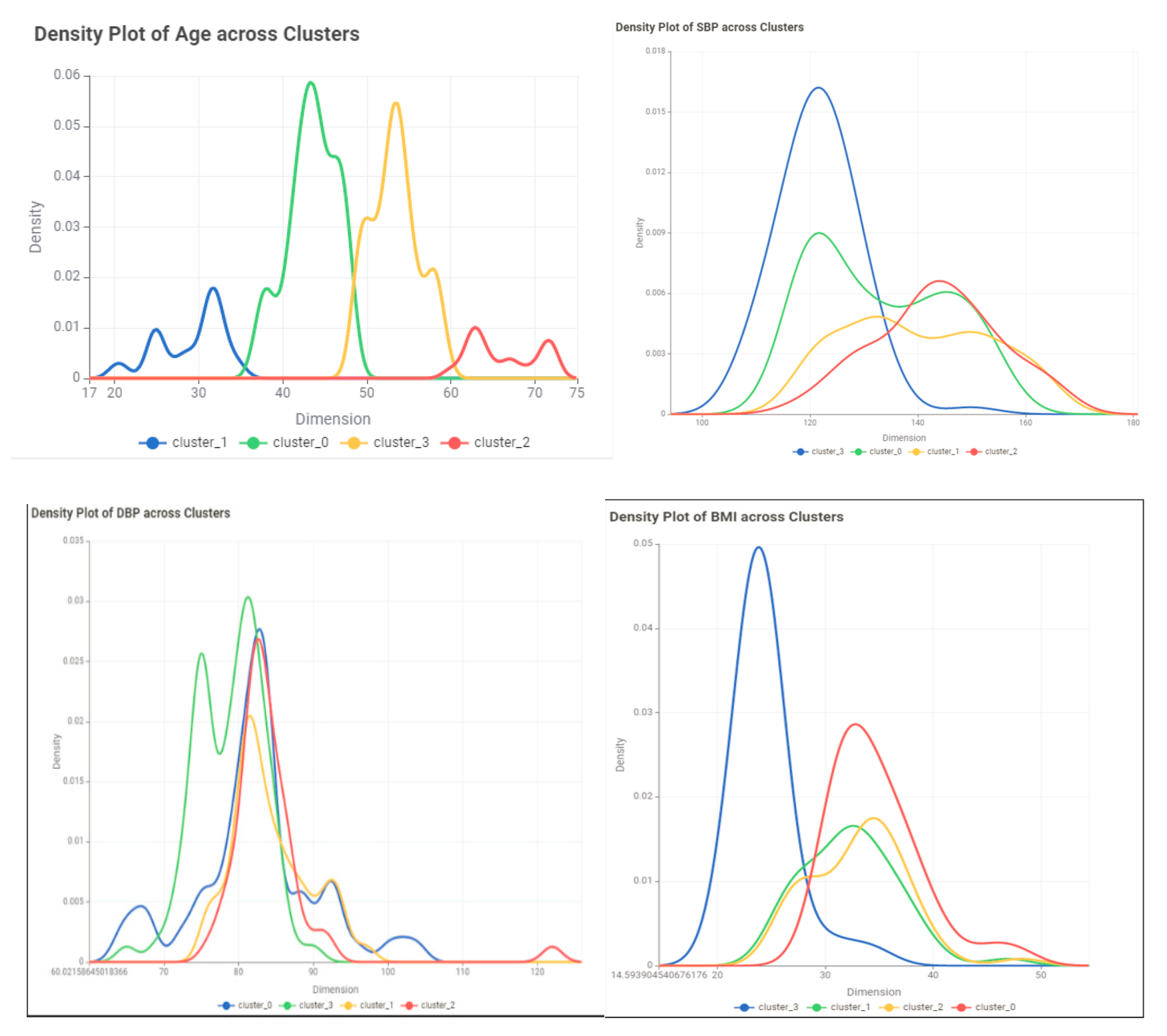
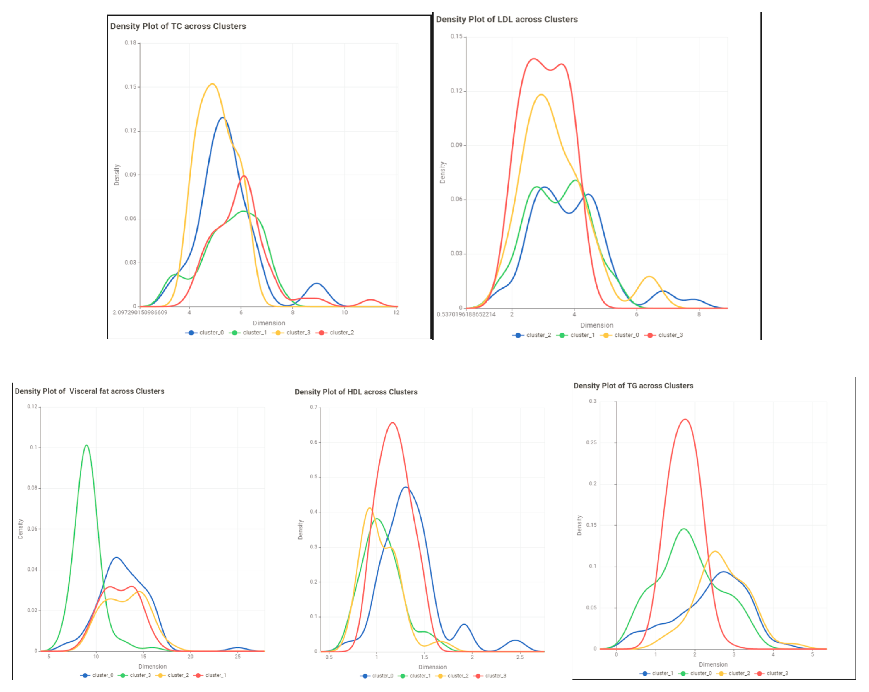
Figures 5 through 13 illustrate density curves that encapsulate a nuanced visual interpretation of the distribution patterns of critical variables including age, systolic and diastolic blood pressure (SBP and DBP), body mass index (BMI), total cholesterol (TC), low-density lipoprotein cholesterol (LDL-C), high-density lipoprotein cholesterol (HDL-C), triglycerides (TG), and visceral adiposity among the four identified clusters. These graphical representations elucidate variations in the prevalence and magnitude of cardiovascular disease (CVD) risk determinants among the clusters.
Conclusion and Discussion
In this study, we explored the efficacy of integrating fuzzy c-means clustering with principal component analysis (PCA) in the investigation of cardiovascular disease (CVD) and obesity. The results affirm the potential of these methodologies to identify vulnerable subgroups within the population and tailor interventions accordingly. Despite their promising utility, our research draws attention to the considerable challenges related to the characteristics of datasets and the selection of analytical parameters, underscoring the necessity for careful execution and rigorous validation procedures. There is a clear need for additional exploration to overcome these barriers, refine these computational techniques, and ensure their seamless integration into clinical practice.
Our thorough analysis reveals that fuzzy c-means clustering and PCA contribute to a deeper insight into the heterogeneity inherent in risk factors for CVD and obesity. This aligns with current scholarly discourse, reinforcing the classification of subjects into distinct clusters to enable targeted public health interventions. However, we must acknowledge the limitations and potential biases present in our investigative approach, advocating for circumspect interpretation and prudent application of these analytic tools. It falls to future research endeavors to further develop these methods, aligning them closely with clinical endpoints to bolster the precision of health intervention strategies.
In conclusion, our investigation highlights that fuzzy c-means clustering and PCA have considerable potential in identifying patterns among voluminous datasets relating to CVD and obesity, thereby informing individualized treatment approaches. Nonetheless, there is an imperative for ongoing inquiry into understanding their constraints and possible predispositions within these domains. Comprehensive evaluations on the application of fuzzy c-means clustering and PCA can facilitate more informed determinations about their capacity to improve prevention and management programs confronting these critical health challenges.
References
- “Cardiovascular diseases (CVDs).” https://www.who.int/news-room/fact-sheets/detail/cardiovascular-diseases-(cvds) (accessed May 19, 2024).
- S. Takeshita et al., “Novel subgroups of obesity and their association with outcomes: a data-driven cluster analysis,” BMC Public Health, vol. 24, no. 1, 2024. [CrossRef]
- R. Vijayarajan and S. Muttan, “Fuzzy C-means clustering based principal component averaging fusion,” Int. J. Fuzzy Syst., vol. 16, no. 2, 2014.
- C. Violán et al., “Soft clustering using real-world data for the identification of multimorbidity patterns in an elderly population: Cross-sectional study in a Mediterranean population,” BMJ Open, vol. 9, no. 8, 2019. [CrossRef]
- C. E. Ndumele et al., “Obesity and Subtypes of Incident Cardiovascular Disease,” J. Am. Heart Assoc., vol. 5, no. 8, 2016. [CrossRef]
- F. B. Ortega, C. J. Lavie, and S. N. Blair, “Obesity and cardiovascular disease,” Circulation Research, vol. 118, no. 11. Lippincott Williams and Wilkins, pp. 1752–1770, May 27, 2016. [CrossRef]
- L. Li, Q. Song, and X. Yang, “K-means clustering of overweight and obese population using quantile-transformed metabolic data,” Diabetes, Metab. Syndr. Obes., vol. 12, 2019. [CrossRef]
- A. Chusyairi and P. R. N. Saputra, “Fuzzy C-Means Clustering Algorithm For Grouping Health Care Centers On Diarrhea Disease,” Int. J. Artif. Intell. Res., vol. 5, no. 1, 2021. [CrossRef]
- B. R. Reddy, Y. Vijay Kumar, and M. Prabhakar, “Clustering large amounts of healthcare datasets using fuzzy c-means algorithm,” in 2019 5th International Conference on Advanced Computing and Communication Systems, ICACCS 2019, 2019. [CrossRef]
- S. Handoyo, A. Widodo, W. H. Nugroho, and I. N. Purwanto, “The implementation of a hybrid fuzzy clustering on the public health facility data,” Int. J. Adv. Trends Comput. Sci. Eng., vol. 8, no. 6, 2019. [CrossRef]
- C. E. Friesen, P. Seliske, and A. Papadopoulos, “Using Principal Component Analysis to Identify Priority Neighbourhoods for Health Services Delivery by Ranking Socioeconomic Status,” Online J. Public Health Inform., vol. 8, no. 2, 2016. [CrossRef]
- E. F. Jackson, A. Siddiqui, H. Gutierrez, A. M. Kanté, J. Austin, and J. F. Phillips, “Estimation of indices of health service readiness with a principal component analysis of the Tanzania Service Provision Assessment Survey,” BMC Health Serv. Res., vol. 15, no. 1, 2015. [CrossRef]
- G. S. M. Khamis and S. M. Alanazi, “Exploring sex disparities in cardiovascular disease risk factors using principal component analysis and latent class analysis techniques,” BMC Med. Inform. Decis. Mak., vol. 23, no. 1, 2023. [CrossRef]
- A. Chatterjee, M. W. Gerdes, and S. G. Martinez, “Identification of risk factors associated with obesity and overweight—a machine learning overview,” Sensors (Switzerland), vol. 20, no. 9, 2020. [CrossRef]
- M. Safaei, E. A. Sundararajan, M. Driss, W. Boulila, and A. Shapi’i, “A systematic literature review on obesity: Understanding the causes & consequences of obesity and reviewing various machine learning approaches used to predict obesity,” Computers in Biology and Medicine, vol. 136. 2021. [CrossRef]
- F. Ferdowsy, K. S. A. Rahi, M. I. Jabiullah, and M. T. Habib, “A machine learning approach for obesity risk prediction,” Curr. Res. Behav. Sci., vol. 2, 2021. [CrossRef]
- M. Negahbani, S. Joulazadeh, H. R. Marateb, and M. Mansourian, “Coronary Artery Disease Diagnosis Using Supervised Fuzzy C-Means with Differential Search Algorithm-based Generalized Minkowski Metrics,” Arch. Biomed. Sci. Eng., 2015. [CrossRef]
- I. J.- Technometrics and undefined 2003, “Principal component analysis,” search.proquest.comIT JolliffeTechnometrics, 2003•search.proquest.com, Accessed: Mar. 14, 2024. [Online]. Available: https://search.proquest.com/openview/759ac31230fa617356d7c8b774ba845e/1?pq-origsite=gscholar&cbl=24108.
- J. Shlens, “A Tutorial on Principal Component Analysis,” Apr. 2014, Accessed: Mar. 14, 2024. [Online]. Available: http://arxiv.org/abs/1404.1100.
- Z. Zhang and A. Castelló, “Principal components analysis in clinical studies,” Ann. Transl. Med., vol. 5, no. 17, 2017. [CrossRef]
- L. Gour et al., “Characterization of rice (Oryza sativa L.) genotypes using principal component analysis including scree plot & rotated component matrix,” ~ 975 ~ Int. J. Chem. Stud., vol. 5, no. 4, 2017.
- Y. Chen, S. Zhou, X. Zhang, D. Li, and C. Fu, “Improved fuzzy c-means clustering by varying the fuzziness parameter,” Pattern Recognit. Lett., vol. 157, 2022. [CrossRef]
- W. Xiao, Y. Zhao, X. Gao, C. Liao, S. Huang, and L. Deng, “Implementation of Fuzzy C-Means (FCM) Clustering Based Camouflage Image Generation Algorithm,” IEEE Access, vol. 9, 2021. [CrossRef]
- K. Zhou and S. Yang, “Effect of cluster size distribution on clustering: a comparative study of k-means and fuzzy c-means clustering,” Pattern Anal. Appl., vol. 23, no. 1, 2020. [CrossRef]
- H. Li, L. Dou, S. Li, Y. Kang, X. Yang, and H. Dong, “Abnormal State Detection of OLTC Based on Improved Fuzzy C-means Clustering,” Chinese J. Electr. Eng., vol. 9, no. 1, 2023. [CrossRef]
- X. Xu, H. Zhang, C. Yang, X. Zhao, and B. Li, “Fairness constraint of Fuzzy C-means Clustering improves clustering fairness,” in Proceedings of Machine Learning Research, 2021.
- C. Wang, W. Pedrycz, J. Bin Yang, M. C. Zhou, and Z. W. Li, “Wavelet Frame-Based Fuzzy C-Means Clustering for Segmenting Images on Graphs,” IEEE Trans. Cybern., vol. 50, no. 9, 2020. [CrossRef]
- E. R. Hruschka and N. F. F. Ebecken, “A genetic algorithm for cluster analysis,” Intell. Data Anal., vol. 7, no. 1, 2003. [CrossRef]
- J. C. Bezdek, Pattern Recognition with Fuzzy Objective Function Algorithms. 1981. [CrossRef]
- P. J. Rousseeuw, “Silhouettes: A graphical aid to the interpretation and validation of cluster analysis,” J. Comput. Appl. Math., vol. 20, no. C, 1987. [CrossRef]
Figure 1.
correlation matrix.
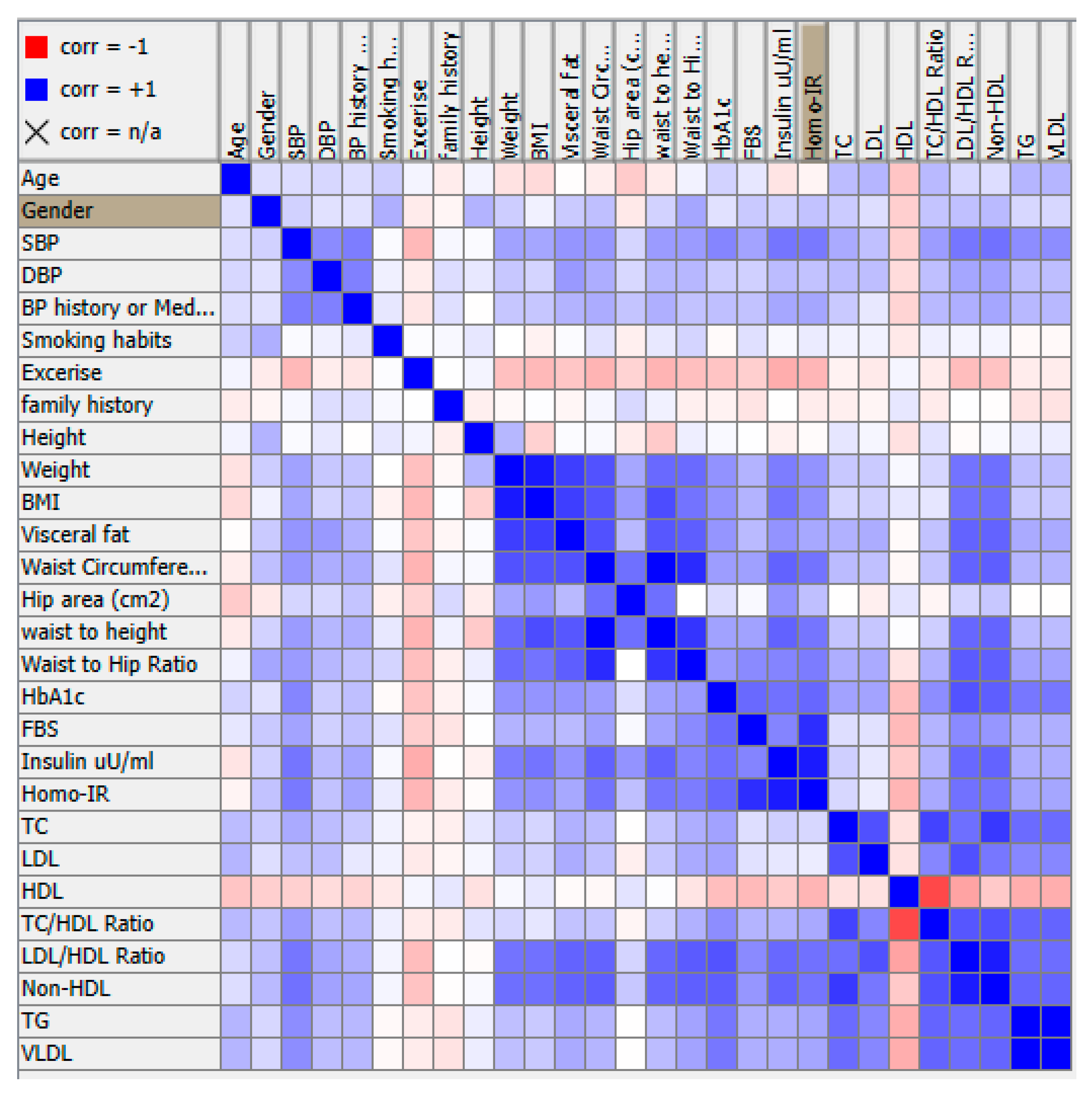
Figure 2.
Correlation circle.
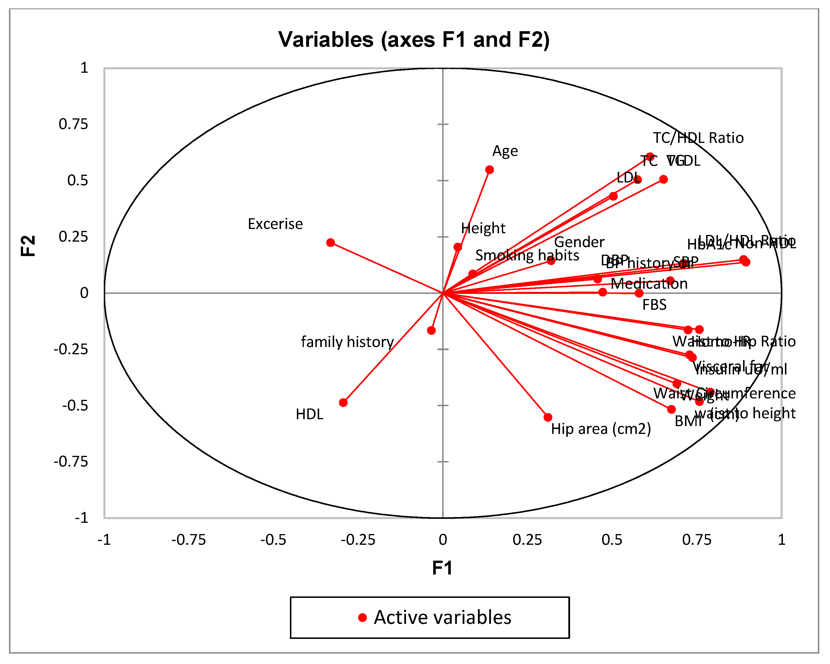
Figure 3.
Scree plot.
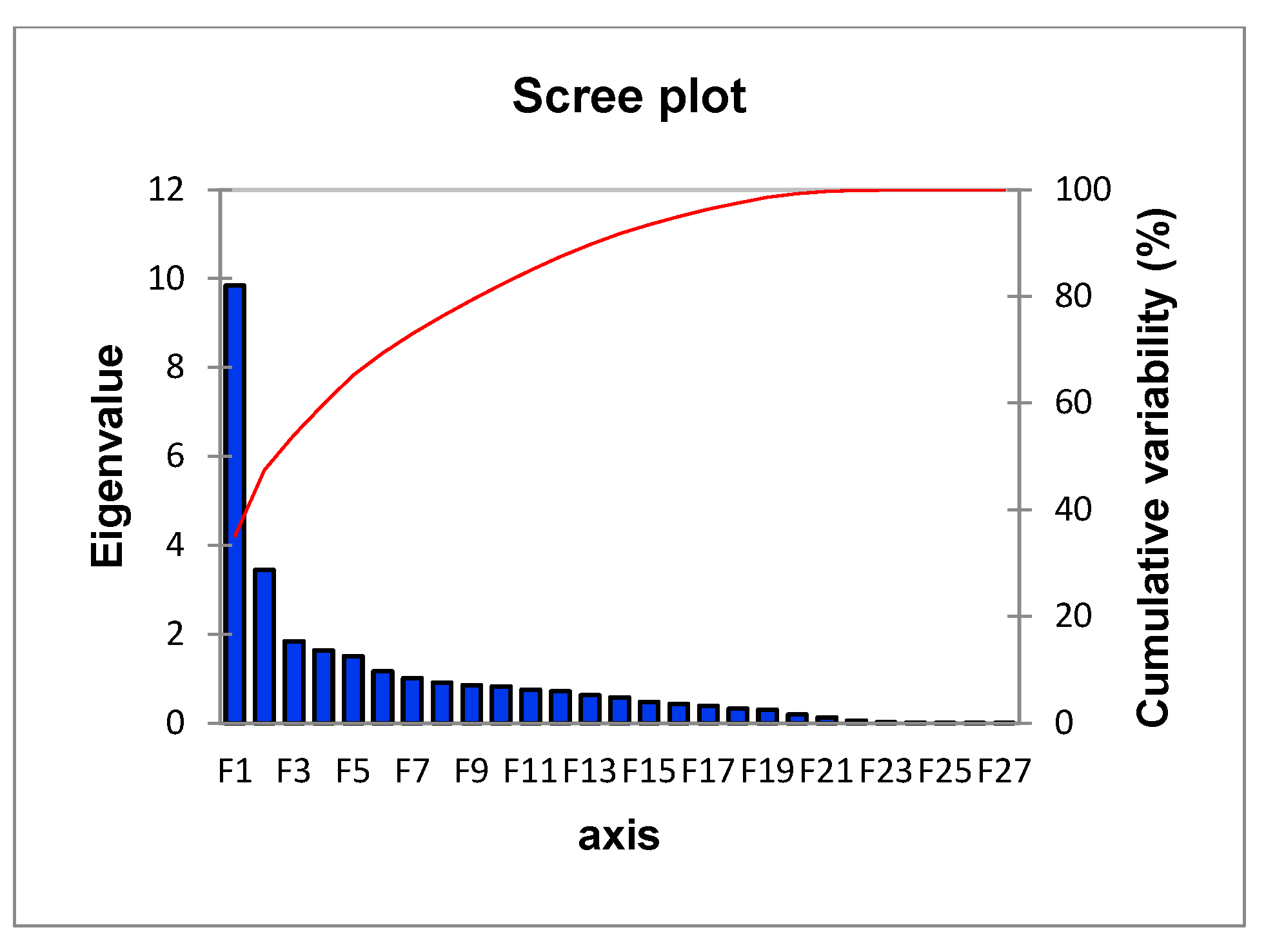
Figure 4.
A graphical representation of the data.
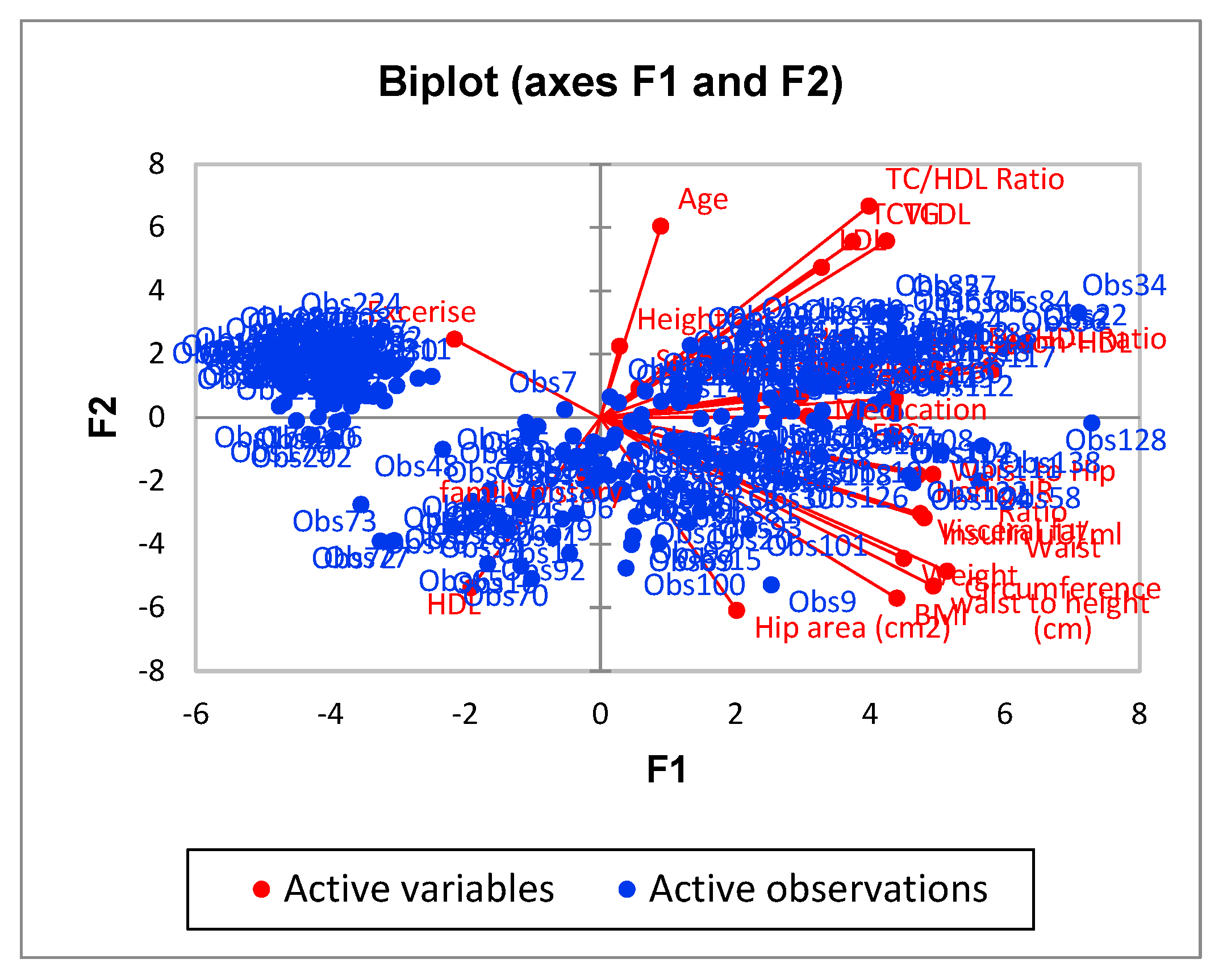
Table 2.
Squared cosines of the variables.
| F1 | F2 | F3 | F4 | F5 | |
|---|---|---|---|---|---|
| Age | 0.019 | 0.301 | 0.000 | 0.014 | 0.030 |
| Gender | 0.102 | 0.021 | 0.035 | 0.436 | 0.003 |
| SBP | 0.451 | 0.003 | 0.024 | 0.025 | 0.081 |
| DBP | 0.209 | 0.004 | 0.002 | 0.000 | 0.379 |
| BP history or Medication | 0.222 | 0.000 | 0.026 | 0.013 | 0.385 |
| Smoking habits | 0.008 | 0.007 | 0.040 | 0.342 | 0.055 |
| Exercise | 0.110 | 0.050 | 0.017 | 0.004 | 0.009 |
| family history | 0.001 | 0.027 | 0.012 | 0.013 | 0.301 |
| Height | 0.002 | 0.042 | 0.003 | 0.311 | 0.001 |
| Weight | 0.477 | 0.162 | 0.039 | 0.050 | 0.025 |
| BMI | 0.456 | 0.268 | 0.052 | 0.002 | 0.033 |
| Visceral fat | 0.530 | 0.075 | 0.093 | 0.021 | 0.000 |
| Waist Circumference (cm) | 0.623 | 0.194 | 0.010 | 0.030 | 0.002 |
| Hip area (cm2) | 0.096 | 0.305 | 0.006 | 0.065 | 0.065 |
| waist to height | 0.574 | 0.232 | 0.011 | 0.002 | 0.001 |
| Waist to Hip Ratio | 0.573 | 0.026 | 0.002 | 0.129 | 0.018 |
| HbA1c | 0.506 | 0.018 | 0.031 | 0.045 | 0.042 |
| FBS | 0.335 | 0.000 | 0.310 | 0.000 | 0.039 |
| Insulin uU/ml | 0.543 | 0.082 | 0.129 | 0.029 | 0.001 |
| Homo-IR | 0.524 | 0.027 | 0.335 | 0.010 | 0.011 |
| TC | 0.330 | 0.254 | 0.166 | 0.000 | 0.000 |
| LDL | 0.253 | 0.185 | 0.227 | 0.001 | 0.004 |
| HDL | 0.087 | 0.237 | 0.206 | 0.001 | 0.000 |
| TC/HDL Ratio | 0.374 | 0.367 | 0.002 | 0.006 | 0.000 |
| LDL/HDL Ratio | 0.788 | 0.022 | 0.012 | 0.002 | 0.007 |
| Non-HDL | 0.801 | 0.019 | 0.031 | 0.002 | 0.001 |
| TG | 0.424 | 0.256 | 0.008 | 0.040 | 0.007 |
| VLDL | 0.424 | 0.256 | 0.008 | 0.040 | 0.007 |
Table 3.
Cluster’s Models Metrics.
| Metrics | BCV | PC | PE | SS | |
|---|---|---|---|---|---|
| Models | |||||
| Model1 | 62.65 | 0.78 | -0.39 | 0.556 | |
| Model2 | 112.96 | 0.77 | -0.43 | 0.575 | |
| Model3 | 81.79 | 0.61 | -0.79 | 0.368 | |
| Variable | Cluster 0 | Cluster1 | Cluster2 | Cluster3 |
| Age | ||||
| Min | 20 | 55 | 47 | 37 |
| Max | 37 | 72 | 56 | 48 |
| Mean | 29.35714 | 61.43243 | 51.49367089 | 43.11957 |
| Std | 4.227023 | 5.35693 | 2.536267284 | 2.724905 |
| Skewness | -0.54403 | 0.838738 | -0.39150176 | -0.33508 |
| Gender | M=15 F=13 | M=32 F=5 | M=46 F=33 | M=61 F=31 |
| SBP | ||||
| Min | 109 | 118 | 110 | 110 |
| Max | 155 | 166 | 163 | 164 |
| Mean | 130.1786 | 142.6757 | 127.2405 | 134.1304 |
| Std | 12.49608 | 12.8799 | 12.13515 | 13.81687 |
| Skewness | 0.395331 | -0.07564 | 1.313037 | 0.202832 |
| DBP | ||||
| Min | 64 | 77 | 72 | 65 |
| Max | 92 | 97 | 104 | 122 |
| Mean | 80.78571 | 86.18919 | 80.43038 | 82.28261 |
| Std | 7.335137 | 5.114456 | 4.637317 | 8.606573 |
| Skewness | -0.93462 | 0.355651 | 1.561946 | 2.131193 |
| BP history or Medication | Yes=3 No=25 | Yes=14 No=23 | Yes= 6 No=73 | Yes=19 No=73 |
| Smoking habits | Yes=8 No=20 | Yes=22 No=15 | Yes=39 No=40 | Yes=39 No=53 |
| Exercise | Yes=2 No=26 | Yes=1 No=36 | Yes=18 No=61 | Yes=6 No=86 |
| family history | Yes=8 No=20 | Yes=7 No=30 | Yes=16 No=63 | Yes=21 No=71 |
| Height | ||||
| Min | 147 | 156 | 149 | 148 |
| Max | 174 | 179 | 182 | 186 |
| Mean | 161.6607 | 165.4054 | 165.3987 | 167.25 |
| Std | 7.557255 | 6.495552 | 6.596123 | 7.900306 |
| Skewness | -0.25755 | 0.772235 | 0.330033 | 0.414278 |
| Weight | ||||
| Min | 67.8 | 67.5 | 52.5 | 55.5 |
| Max | 106.3 | 109.5 | 111 | 146 |
| Mean | 87.88214 | 89.56216 | 73.22532 | 89.57446 |
| Std | 10.54785 | 11.10384 | 13.75203 | 17.05227 |
| Skewness | 0.048747 | -0.22378 | 0.925506 | 0.607339 |
| BMI | ||||
| Min | 26.89232 | 25.43615992 | 20.904195 | 20.8326039 |
| Max | 45.21264 | 40.7712239 | 40.009145 | 48.2230149 |
| Mean | 33.73876 | 32.7276647 | 26.776844 | 32.0996482 |
| Std | 4.420732 | 3.622917706 | 4.9167259 | 6.07196575 |
| Skewness | 0.382043 | 0.112175598 | 1.1975546 | 0.36958127 |
| Visceral fat | ||||
| Min | 7 | 9 | 7 | 7 |
| Max | 16 | 16 | 16 | 25 |
| Mean | 12.14285714 | 13.189189 | 10.2658228 | 12.06522 |
| Std | 2.383807812 | 1.7769799 | 2.35180706 | 2.843169 |
| Skewness | -0.535412896 | -0.3651297 | 1.21897441 | 1.114398 |
| Waist Circumference | ||||
| Min | 87 | 87 | 64 | 69 |
| Max | 138 | 147 | 147 | 147 |
| Mean | 112.57143 | 112.405405 | 93.08861 | 105.6522 |
| Std | 14.325395 | 13.2171174 | 17.31769 | 17.71783 |
| Skewness | -0.0402391 | 0.46329165 | 0.992768 | 0.140572 |
| Hip area | ||||
| Min | 84 | 89 | 87 | 84 |
| Max | 134 | 135 | 128 | 141 |
| Mean | 114.178571 | 106.5135 | 102.6203 | 107.2826 |
| Std | 11.6047678 | 10.79254 | 8.557953 | 11.63863 |
| Skewness | -1.1293167 | 0.84846 | 0.701783 | 0.536408 |
| waist to height | ||||
| Min | 0.54717 | 0.486034 | 0.402516 | 0.417143 |
| Max | 0.857143 | 0.896341 | 0.924528 | 0.898649 |
| Mean | 0.695705 | 0.680444 | 0.562661 | 0.632907 |
| Std | 0.077757 | 0.082398 | 0.109548 | 0.110671 |
| Skewness | 0.312657 | 0.25963 | 1.074341 | 0.133961 |
| Waist to Hip Ratio | ||||
| Min | 0.756098 | 0.820313 | 0.719101 | 0.75 |
| Max | 1.201754 | 1.373626 | 1.441176 | 1.277228 |
| Mean | 0.990768 | 1.058794 | 0.905315 | 0.986079 |
| Std | 0.1193 | 0.107614 | 0.143132 | 0.136749 |
| Skewness | -0.56083 | 0.053912 | 1.406808 | -0.05666 |
| FBS | ||||
| Min | 72.54 | 92.16 | 76 | 76 |
| Max | 230 | 340 | 244 | 239 |
| Mean | 132.8143 | 157.7381 | 113.4273 | 124.8425 |
| Std | 47.14809 | 56.44463 | 36.83982 | 41.7015 |
| Skewness | 0.835888 | 1.146436 | 1.815943 | 1.273658 |
| Insulin uU/ml | ||||
| Min | 7 | 8.4 | 5.3 | 5.3 |
| Max | 37.37 | 37.7 | 35.07 | 35.93 |
| Mean | 20.66893 | 21.09784 | 11.52722 | 18.01489 |
| Std | 7.387154 | 7.788241 | 8.111252 | 8.284636 |
| Skewness | 0.222751 | 0.176514 | 1.211076 | -0.03373 |
| Homo-IR | ||||
| Min | 1.362667 | 2.645618 | 1.102716 | 1.04 |
| Max | 14.46667 | 15.60593 | 17.17037 | 16.74815 |
| Mean | 7.115011 | 7.972435 | 3.743428 | 6.046711 |
| Std | 3.965715 | 3.516842 | 3.843697 | 4.061748 |
| Skewness | 0.471698 | 0.556379 | 1.665274 | 0.685207 |
| TC | ||||
| Min | 3.39 | 4.44792 | 3.17 | 3.16 |
| Max | 6.8529 | 9.24 | 7.43 | 11.01 |
| Mean | 5.031471 | 6.206487 | 5.22029 | 5.516702 |
| Std | 0.954634 | 1.185539 | 0.785381 | 1.186209 |
| Skewness | 0.078733 | 1.146114 | 0.228108 | 1.234394 |
| LDL | ||||
| Min | 1.65 | 2.40498 | 1.6 | 1.68 |
| Max | 4.92 | 6.63 | 5.25 | 7.85 |
| Mean | 2.99725 | 4.268808 | 3.204681 | 3.337668 |
| Std | 0.844356 | 1.07715 | 0.740261 | 1.090519 |
| Skewness | 0.493168 | 0.408088 | 0.052199 | 1.440394 |
| TC/HDL Ratio | ||||
| Min | 1.92 | 3.265734 | 2.381503 | 2.198675 |
| Max | 7.117647 | 9.275862 | 9.137931 | 9.54023 |
| Mean | 3.956313 | 5.911426 | 4.587839 | 4.987292 |
| Std | 1.337887 | 1.330685 | 1.168956 | 1.647908 |
| Skewness | 0.834276 | -0.04545 | 1.448609 | 0.734131 |
| LDL/HDL Ratio | ||||
| Min | 1.192 | 2.067164 | 0.404765 | 0.354619 |
| Max | 4.472727 | 5.724138 | 5.133333 | 7.816092 |
| Mean | 2.347742 | 4.047246 | 1.4837 | 2.624972 |
| Std | 0.908145 | 1.049943 | 1.174594 | 1.592378 |
| Skewness | 0.79823 | -0.35873 | 1.31546 | 0.667992 |
| Non-HDL | ||||
| Min | 2.16 | 3.24 | 0.98773 | 1.242647 |
| Max | 5.76678 | 7.93 | 6.10296 | 9.41 |
| Mean | 3.680818 | 5.130117 | 2.59537 | 3.886513 |
| Std | 1.074989 | 1.176047 | 1.461076 | 1.605203 |
| Skewness | 0.393767 | 0.794324 | 0.904014 | 0.514697 |
| TG | ||||
| Min | 0.42 | 1.56 | 0.69 | 0.41 |
| Max | 3.31926 | 3.9 | 4.23 | 4.54 |
| Mean | 1.525748 | 2.586565 | 1.930973 | 2.169234 |
| Std | 0.845067 | 0.637059 | 0.600044 | 0.816264 |
| Skewness | 0.814079 | 0.127149 | 1.154205 | 0.11867 |
| VLDL | ||||
| Min | 0.190909 | 0.709091 | 0.313636 | 0.186364 |
| Max | 1.508755 | 1.772727 | 1.922727 | 2.063636 |
| Mean | 0.693522 | 1.175711 | 0.877715 | 0.986015 |
| Std | 0.384121 | 0.289572 | 0.272747 | 0.371029 |
| Skewness | 0.814079 | 0.127149 | 1.154205 | 0.11867 |
| HDL | ||||
| Min | 0.7 | 0.67 | 0.87924 | 0.63 |
| Max | 2.4 | 1.73 | 2.5 | 2.725942 |
| Mean | 1.179515 | 1.134267 | 1.359937 | 1.363539 |
| Std | 0.263488 | 0.207883 | 0.341299 | 0.03568 |
| Skewness | 1.378342 | 0.275384 | 1.63957 | 1.394629 |
Disclaimer/Publisher’s Note: The statements, opinions and data contained in all publications are solely those of the individual author(s) and contributor(s) and not of MDPI and/or the editor(s). MDPI and/or the editor(s) disclaim responsibility for any injury to people or property resulting from any ideas, methods, instructions or products referred to in the content. |
© 2024 by the authors. Licensee MDPI, Basel, Switzerland. This article is an open access article distributed under the terms and conditions of the Creative Commons Attribution (CC BY) license (http://creativecommons.org/licenses/by/4.0/).
Copyright: This open access article is published under a Creative Commons CC BY 4.0 license, which permit the free download, distribution, and reuse, provided that the author and preprint are cited in any reuse.


