Tutorial on Deep Generative Model

1. Introduction to Deep Generative Model (DGM)

By informal statement, generative artificial intelligence (GenAI) applications aim to reproduce original artifacts such as images, sounds, music, texts, and speeches into a new artifact with some changes. The problem is that reproduction or generation, which is not duplication, indeed derives a new piece of content which is large or small from whole content of the original artifacts. For example, given a smiling face of a specific person, GenAI application will generate a crying face of the same person. As a subdomain of GenAI, deep generative model (DGM) applies deep neural network (DNN) into generating artifacts but many deep generative models (DGMs) are also relevant to applied statistics. Note, DNN is an artificial neural network having many hidden layers, besides input layer and output layer. Training deep neural network or learning deep neural network is known as deep learning. Given random variable vector x = (x₁, x₂,…, x_m)^T presenting any digital artifact or any digital data such as image and sound, let P(x) be probability density function (PDF) of x but it is difficult to estimate such probabilistic distribution P(x) because data x is complicated with suppose that x belongs to the real field R^m where m is high dimension and so, P(x) is called intractable PDF. Suppose there is another random variable vector z = (z₁, z₂,…, z_n)^T belonging to the real field Rⁿ where n is low dimension (n < m) so that PDF of z denoted P(z) is tractable and it is possible to understand P(z). Moreover, it is most important that suppose there is a function g(z | Φ) = x that maps tractable data z to intractable data x where Φ is parameter of such mapping function. For some illustrations or examples in this report, random variable vector x is flattened from two-dimension image. As a convention, the function g(z | Φ) = x is called generator of x and its parameter Φ is called generator parameter (Ruthotto & Haber, 2021, p. 2).

$$g:R^n\to R^m\mathrm{s}\mathrm{u}\mathrm{c}\mathrm{h} \mathrm{t}\mathrm{h}\mathrm{a}\mathrm{t}\mathit{x}=g\left(\mathit{z}|\mathsf{\Phi }\right)\mathrm{w}\mathrm{h}\mathrm{e}\mathrm{r}\mathrm{e}\mathit{z}\in Z\subseteq R^n,\mathit{x}\in X\subseteq R^m$$

Where Z and X are domains of tractable data x and intractable data z with note that Z is called latent space and X is called sample space by convention. When Z is called latent space, tractable PDF P(z) is called latent distribution. Because g(z | Φ) is essentially vector-by-vector function whose input and output are vectors, it should have denoted as g(z | Φ). However, it is still denoted g(z | Φ) in context DNN because there are two reasons: 1) g(z | Φ) is not bijection and 2) the output x of g(z | Φ) can be considered as scalar variable x corresponding to an output neuron of output layer in neural network. Therefore, g(z | Φ) also implies a vector-by-scalar function whose first-order derivative can be considered as gradient vector although the first-order derivative of vector-by-vector function g(z | Φ) is Jacobian matrix. Note, in mathematical, the first-order derivative of scalar-by-vector function is called gradient vector and the first-order derivative of vector-by-vector function is called Jacobian matrix.

The ultimate purpose of any DGM is to determine parameter Φ because generator g(z | Φ) is defined based on Φ. In DGM, generator g(z | Φ) is constructed by a deep neural network (DNN) and its parameter Φ is essentially weights of such DNN. When g(z | Φ) is constructed by DNN, g(z | Φ) is not totally equal to x as g(z | Φ) = x but it is expected that g(z | Φ) is approximated to x in practice:

$$g\left(\mathit{z}|\mathsf{\Phi }\right)={\mathit{x}}^{\prime }\cong \mathit{x}$$

Note that there are many DGMs and some of them do not require explicit definition of the PDF P(z) of tractable data z but how to estimate generator parameter Φ for determining generator g(z | Φ) = x is always concerned. When g(z | Φ) was determined, we can easily randomize some random tractable data z’ according to the known tractable PDF P(z) and then it is totally possible to generate new artifact x’ by x’ = g(z’ | Φ) so that x’ is generated data / derived data of original intractable data x with expectation that probability distribution of x’ is approximate to the true distribution P(x) of x. The process to randomize z’ is called sampling tractable data (z). When g(z | Φ) is modeled by a DNN, how to estimate parameter Φ is essentially to train such DNN and hence, the DNN is denoted as generator function g(z | Φ) for a convention, which is called generator DNN g(z | Φ). Here we identify generator function with DNN.

Intractable PDF P(x) of x is specified (Ruthotto & Haber, 2021, p. 3) based on law of total probability as follows:

$$P\left(\mathit{x}\right)=\underset{\mathit{z}}{\int }{P}_g\left(\mathit{x}|\mathit{z}\right)P\left(\mathit{z}\right)d\mathit{z}$$

Where P_g(x | z) is conditional PDF of x given z, which implies that P_g(x | z) depends on generator g(z | Φ) too because random variable x inside condition PDF P_g(x | z) is generated from z. Note, notation P(.) denotes probability distribution or probability density function (PDF) in this research. Therefore, it is possible to denote such conditional PDF as P(x | Φ, z).

$$P_g\left(\mathit{x}|\mathit{z}\right)=P\left(\mathit{x}|\mathsf{\Phi },\mathit{z}\right)$$

Such that:

$$P\left(\mathit{x}\right)=\underset{\mathit{z}}{\int }P\left(\mathit{x}|\mathsf{\Phi },\mathit{z}\right)P\left(\mathit{z}\right)d\mathit{z}$$

(1.1)

This implies intractable PDF P(x) can be known via tractable PDF P(z) and conditional PDF P(x | Φ, z); however it is really difficult to compute P(x) due to complication of the integral but this difficulty is unimportant because the purpose of DGM is to estimate generator g(z | Φ). As a convention, the conditional PDF P(x | Φ, z) is called likelihood P(x | Φ, z). Indeed, P(x | Φ, z) is likelihood function of intractable data x given tractable data z, which indicates how close generated data x’ = g(z | Φ) to x. In practice tractable PDF P(z) is predefined and likelihood P(x | Φ, z) is determined based on generator DNN g(z | Φ). For instance, P(x | Φ, z) is assumed to be normal distribution (Gaussian distribution) with mean μ and variance σ² in popular as follows (Ruthotto & Haber, 2021, p. 3):

$$P\left(\mathit{x}|\mathsf{\Phi },\mathit{z}\right)={\left(2\pi {\sigma }^2\right)}^{-\frac{m}{2}}\mathrm{e}\mathrm{x}\mathrm{p}\left(-\frac{{‖g\left(\mathit{z}|\mathsf{\Phi }\right)-\mathit{x}-\mathit{\mu }‖}^2}{2{\sigma }^2}\right)$$

Let μ = 0 and σ²=1 for optimization, we have:

$$P\left(\mathit{x}|\mathsf{\Phi },\mathit{z}\right)={\left(2\pi \right)}^{-\frac{m}{2}}\mathrm{e}\mathrm{x}\mathrm{p}\left(-\frac{{‖g\left(\mathit{z}|\mathsf{\Phi }\right)-\mathit{x}-\mathit{\mu }‖}^2}{2}\right)$$

Where notation ||.|| denotes norm of vector. For instance, Euclidean norm of intractable data x is:

$$‖\mathit{x}‖=\sqrt{x_1^2+x_2^2+\dots +x_m^2}$$

That tractable PDF P(z) is predefined (constant with regard to Φ and x) and likelihood P(x | Φ, z) is assumed to distribute normally indicates that intractable PDF P(x) is implied by the simpler conditional PDF P(x | Φ, z) with support of generator DNN g(z | Φ); in other words, P(x | Φ, z) is probability distribution of x from viewpoint of DNN g(z | Φ) indeed where z is totally determined in latent space Z and P(x | Φ, z) is really simpler with support of DNN g(z | Φ). Because how to determine generator g(z | Φ) is to estimate parameter Φ, it is easy to calculate Φ as maximizer of likelihood P(x | Φ, z), which is the optimization problem as follows:

$${\mathsf{\Phi }}^{*}=\underset{\mathsf{\Phi }}{\mathrm{armax}}P\left(\mathit{x}|\mathsf{\Phi },\mathit{z}\right)$$

(1.2)

Taking natural logarithm of likelihood P(x | Φ, z) aims to easily determine Φ by maximizing the log-likelihood function log(P(x | Φ, z)) as follows:

$${\mathsf{\Phi }}^{*}=\underset{\mathsf{\Phi }}{\mathrm{armax}}P\left(\mathit{x}|\mathsf{\Phi },\mathit{z}\right)=\underset{\mathsf{\Phi }}{\mathrm{armax}}\left(\log P\left(\mathit{x}|\mathsf{\Phi },\mathit{z}\right)\right)=\underset{\mathsf{\Phi }}{\mathrm{armax}}\left(-\frac{1}{2}{‖g\left(\mathit{z}|\mathsf{\Phi }\right)-\mathit{x}‖}^2\right)$$

Note,

$$\log P\left(\mathit{x}|\mathsf{\Phi },\mathit{z}\right)=-\frac{m}{2}\log \left(2\pi {\sigma }^2\right)-\frac{{‖g\left(\mathit{z}|\mathsf{\Phi }\right)-\mathit{x}-\mathit{\mu }‖}^2}{2{\sigma }^2}$$

Let μ = 0 and σ²=1 for optimization, we have:

$$\log P\left(\mathit{x}|\mathsf{\Phi },\mathit{z}\right)=-\frac{m}{2}\log \left(2\pi \right)-\frac{{‖g\left(\mathit{z}|\mathsf{\Phi }\right)-\mathit{x}‖}^2}{2}$$

This implies the minimization problem as follows:

$${\mathsf{\Phi }}^{*}=\underset{\mathsf{\Phi }}{\mathrm{armin}}\frac{1}{2}{‖g\left(\mathit{z}|\mathsf{\Phi }\right)-\mathit{x}‖}^2$$

As a result, the estimation of generator parameter Φ based on maximum likelihood estimation (MLE) with assumption of normal distribution of generator g(z | Φ) turns back minimization of error function ½||g(z | Φ) – x||² which is popular technique in learning DNN by backpropagation algorithm because ½||g(z | Φ) – x||² is, indeed, quadratic error function in neural network where g(z | Φ) and x are output and real output of a neuron, respectively with note that the output g(z | Φ) is calculated by propagation rule and the real output x is from training data. In other words, MLE is entry point to estimate generator parameter Φ which is weights of DNN g(z | Φ) that is learned fully by backpropagation algorithm (Nguyen, 2023, pp. 8-20). Therefore, please pay attention to the association of MLE and backpropagation algorithm for determining totally generator g(z | Φ), in which g(z | Φ) and x are output at real output of neurons at the output layer of DNN so that backpropagation algorithm can be applied successively. Note, error function is also called loss function. Backpropagation algorithm is often associated with stochastic gradient descent (SGD) method to optimize loss function.

Let ∇P(x | Φ, z) be gradient of likelihood P(x | Φ, z) which is first-order derivative of P(x | Φ, z) with regard to parameter Φ where x and z are samples as follows:

$$\nabla P\left(\mathit{x}|\mathsf{\Phi },z\right)=\frac{dP\left(\mathit{x}|\mathsf{\Phi },z\right)}{d\mathsf{\Phi }}$$

Stochastic gradient descent (SGD) method (Nguyen, 2023, pp. 22-27) estimates Φ by iterative process to update successively Φ at every iteration as follows:

$$\mathsf{\Phi }=\mathsf{\Phi }+\gamma \nabla P\left(\mathit{x}|\mathsf{\Phi },z\right)$$

Where 0 < γ ≤ 1 is learning rate. SGD, which is an iterative process, pushes candidate solution at each iteration along the direction which is opposite to gradient of target function for minimization or has the same direction to gradient of target function for maximization with note that the step length is represented by learning rate. In practice, likelihood P(x | Φ, z) is replaced by its natural logarithm as follows:

$$\mathsf{\Phi }=\mathsf{\Phi }+\gamma \nabla \log P\left(\mathit{x}|\mathsf{\Phi },\mathit{z}\right)$$

(1.3)

Where ∇P(x | Φ, z) is gradient of the log-likelihood function logP(x | Φ, z) with regard to Φ. Note the estimation equation above mentions maximization problem according to MLE method and hence, if error function denoted ε(x | Φ, z) which is the function related to g(z | Φ) and x like ε(x | Φ, z) = ½||g(z | Φ) – x||² aforementioned, then SGD modifies a little bit the estimation equation as follows:

$$\mathsf{\Phi }=\mathsf{\Phi }-\gamma \nabla \epsilon \left(\mathit{x}|\mathsf{\Phi },\mathit{z}\right)$$

(1.4)

Where ∇ε(x | Φ, z) is gradient of error ε(x | Φ, z).

$$\nabla \epsilon \left(\mathit{x}|\mathsf{\Phi },z\right)=\frac{d\epsilon \left(\mathit{x}|\mathsf{\Phi },z\right)}{d\mathsf{\Phi }}$$

The main difference between maximizing likelihood P(x | Φ, z) and minimizing error ε(x | Φ, z) is the changing from the sign “+” regarding maximization problem to the sign “–” regarding minimization problem, which is the essence of gradient descent method. In the example of assuming normal distribution, likelihood maximization is the same to error minimization but likelihood maximization gives broader applications to estimate generator parameter Φ within context of DNN along with backpropagation algorithm to train DNN. Besides, it is possible to consider error function is the minus opposite of likelihood function:

$$\epsilon \left(\mathit{x}|\mathsf{\Phi },z\right)=-P\left(\mathit{x}|\mathsf{\Phi },\mathit{z}\right)$$

It is better that error is the minus opposite of log-likelihood function:

$$\epsilon \left(\mathit{x}|\mathsf{\Phi },z\right)=-\log P\left(\mathit{x}|\mathsf{\Phi },\mathit{z}\right)$$

Moreover, there many ways to define likelihood and error and so, the way to define them will contribute to form a concrete DGM, besides how to specify and design generator DNN g(z | Φ). When Φ is weight vector consisting of many weights of entire DNN, only elemental sub-weights at the output layer are estimated by SGD which maximizes likelihood or minimizes error:

$${\mathsf{\Phi }}_{\mathrm{o}\mathrm{u}\mathrm{t}\mathrm{p}\mathrm{u}\mathrm{t}}={\mathsf{\Phi }}_{\mathrm{o}\mathrm{u}\mathrm{t}\mathrm{p}\mathrm{u}\mathrm{t}}+\gamma \nabla P\left(\mathit{x}|\mathsf{\Phi },z\right)$$

Or

$${\mathsf{\Phi }}_{\mathrm{o}\mathrm{u}\mathrm{t}\mathrm{p}\mathrm{u}\mathrm{t}}={\mathsf{\Phi }}_{\mathrm{o}\mathrm{u}\mathrm{t}\mathrm{p}\mathrm{u}\mathrm{t}}-\gamma \nabla \epsilon \left(\mathit{x}|\mathsf{\Phi },\mathit{z}\right)$$

Then backpropagation algorithm continues to update remaining sub-weights at hidden layers based on such determined sub-weights at the output layer. Therefore, for convenience, we only focus on likelihood maximization or error minimization and parameter Φ represents entire weights of DNN with assertion that backpropagation algorithm is always feasible. It means that there are two important equivalent estimation equations as follows:

$$\begin{gathered} \mathsf{\Phi }=\mathsf{\Phi }+\gamma \nabla P\left(\mathit{x}|\mathsf{\Phi },\mathit{z}\right) \\ \mathsf{\Phi }=\mathsf{\Phi }-\gamma \nabla \epsilon \left(\mathit{x}|\mathsf{\Phi },\mathit{z}\right) \end{gathered}$$

In similar to:

$$\mathsf{\Phi }=\mathsf{\Phi }+\gamma \nabla \log P\left(\mathit{x}|\mathsf{\Phi },\mathit{z}\right)$$

When DGM is trained with big data, training data is fed to DGM at very time point i as a pair d⁽ⁱ⁾ = (x⁽ⁱ⁾, z⁽ⁱ⁾) and therefore, a set of pairs over N time points is called epoch. As a convention, epoch of size N is denoted as D = (d⁽¹⁾ = (x⁽¹⁾, z⁽¹⁾), d⁽²⁾ = (x⁽²⁾, z⁽²⁾),…, d^(N) = (x^(N), z^(N))). An interesting result from SGD is that DGM can be learned with epoch D without significant change as follows:

$$\mathsf{\Phi }=\mathsf{\Phi }+\gamma \nabla \frac{1}{N}{\displaystyle \sum _{i=1}^N}P\left({\mathit{x}}^{\left(i\right)}|\mathsf{\Phi },{\mathit{z}}^{\left(i\right)}\right)=\mathsf{\Phi }+\gamma \frac{1}{N}{\displaystyle \sum _{i=1}^N}\nabla P\left({\mathit{x}}^{\left(i\right)}|\mathsf{\Phi },{\mathit{z}}^{\left(i\right)}\right)$$

Therefore, training data is counted according to every epoch D instead of every pair (x, z) so that D is fed to SGD at every time point k. Moreover, it is essential that SGD aims to update current parameter at current iteration based on previous parameter at previous iteration. Exactly, let Φ^(k+1) be generator parameter at the (k+1)^th iteration, then Φ^(k+1) is calculated based on previous generator parameter Φ^(k) at the k^th iteration as follows:

$${\mathsf{\Phi }}^{\left(k+1\right)}={\mathsf{\Phi }}^{\left(k\right)}+\gamma \nabla \frac{1}{N}{\displaystyle \sum _{i=1}^N}P\left({\mathit{x}}^{\left(i\right)}|{\mathsf{\Phi }}^{\left(k\right)},{\mathit{z}}^{\left(i\right)}\right)$$

The equation above is the most precise equation for parameter estimation with SGD, which is called epoch estimation with note that SGD is an iterative process. It can also be replaced by following equations:

$$\begin{gathered} {\mathsf{\Phi }}^{\left(k+1\right)}={\mathsf{\Phi }}^{\left(k\right)}+\gamma \nabla \frac{1}{N}{\displaystyle \sum _{i=1}^N}\log P\left({\mathit{x}}^{\left(i\right)}|{\mathsf{\Phi }}^{\left(k\right)},{\mathit{z}}^{\left(i\right)}\right) \\ {\mathsf{\Phi }}^{\left(k+1\right)}={\mathsf{\Phi }}^{\left(k\right)}-\gamma \nabla \frac{1}{N}{\displaystyle \sum _{i=1}^N}\epsilon \left({\mathit{x}}^{\left(i\right)}|{\mathsf{\Phi }}^{\left(k\right)},{\mathit{z}}^{\left(i\right)}\right) \end{gathered}$$

The first equation

$${\mathsf{\Phi }}^{\left(k+1\right)}={\mathsf{\Phi }}^{\left(k\right)}+\gamma \nabla \frac{1}{N}{\displaystyle \sum _{i=1}^N}\log P\left({\mathit{x}}^{\left(i\right)}|{\mathsf{\Phi }}^{\left(k\right)},{\mathit{z}}^{\left(i\right)}\right)$$

(1.5)

Which is most popular. Moreover, the index k indicates time point as well as iteration of SGD. If learning rate γ is varied at every iteration as γ^(k), we have:

$${\mathsf{\Phi }}^{\left(k+1\right)}={\mathsf{\Phi }}^{\left(k\right)}+{\gamma }^{\left(k\right)}\nabla \frac{1}{N}{\displaystyle \sum _{i=1}^N}\log P\left({\mathit{x}}^{\left(i\right)}|{\mathsf{\Phi }}^{\left(k\right)},{\mathit{z}}^{\left(i\right)}\right)$$

There are two problems related to construct a DGM: 1) how to define likelihood or error to train generator DNN g(z | Φ) and 2) how to define tractable PDF P(z) which implies the way to randomize z. The second problem relates to assert qualification of random data z’ and hence, the second problem is stated as qualification problem of how to qualify random data. Therefore, the two problems of constructing DGM are 1) how to train generator DNN g(z | Φ) and 2) how to qualify such training task which often relates to another optimization task or another training task. Some basic principles related to DGM are introduced in this section but the two problems cannot be mentioned because there are many specific DGMs which have own specifications. Anyhow generator likelihood P(x | Φ, z) based on definition of generator g(z | Φ) is always important regardless that if it is specified explicitly and thus, suppose it was defined, then SGD is favorite method to optimize it. As an example aforementioned, suppose P(x | Φ, z) distributes normally with mean μ and variance σ² in some DGM as follows (Ruthotto & Haber, 2021, p. 3):

$$P\left(\mathit{x}|\mathsf{\Phi },\mathit{z}\right)={\left(2\pi {\sigma }^2\right)}^{-\frac{m}{2}}\mathrm{e}\mathrm{x}\mathrm{p}\left(-\frac{{‖g\left(\mathit{z}|\mathsf{\Phi }\right)-\mathit{x}-\mathit{\mu }‖}^2}{2{\sigma }^2}\right)$$

Generator log-likelihood is natural logarithm of generator likelihood P(x | Φ, z):

$$\log P\left(\mathit{x}|\mathsf{\Phi },\mathit{z}\right)=-\frac{m}{2}\log \left(2\pi {\sigma }^2\right)-\frac{{‖g\left(\mathit{z}|\mathsf{\Phi }\right)-\mathit{x}-\mathit{\mu }‖}^2}{2{\sigma }^2}$$

Gradient of this log-likelihood with regard to Φ is:

$$\nabla \log P\left(\mathit{x}|\mathsf{\Phi },\mathit{z}\right)=\frac{d\log P\left(\mathit{x}|\mathsf{\Phi },\mathit{z}\right)}{d\mathsf{\Phi }}=-\frac{\left(g\left(\mathit{z}|\mathsf{\Phi }\right)-\mathit{x}-\mathit{\mu }\right)}{{\sigma }^2}\frac{dg\left(\mathit{z}|\mathsf{\Phi }\right)}{d\mathsf{\Phi }}$$

Where dg(z | Φ) / dΦ is differential of g(z | Φ) with regard to Φ. Let μ = 0 and σ²=1 for optimization, we have:

$$\nabla \log P\left(\mathit{x}|\mathsf{\Phi },\mathit{z}\right)=\frac{d\log P\left(\mathit{x}|\mathsf{\Phi },\mathit{z}\right)}{d\mathsf{\Phi }}=-\left(g\left(\mathit{z}|\mathsf{\Phi }\right)-\mathit{x}\right)\frac{dg\left(\mathit{z}|\mathsf{\Phi }\right)}{d\mathsf{\Phi }}$$

As usual, estimation equation resulted from SGD is:

$$\mathsf{\Phi }=\mathsf{\Phi }+\gamma \nabla \log P\left(\mathit{x}|\mathsf{\Phi },\mathit{z}\right)=\mathsf{\Phi }+\gamma \left(\mathit{x}-g\left(\mathit{z}|\mathsf{\Phi }\right)\right)\frac{dg\left(\mathit{z}|\mathsf{\Phi }\right)}{d\mathsf{\Phi }}$$

There is a question that how to calculate the differential dg(z | Φ) / dΦ. Indeed, it is not difficult to calculate it in context of neural network associated with backpropagation algorithm so that the last output layer as well as last neuron o of DNN g(z | Φ) is acted by activation function a(.) as follows:

$$\begin{gathered} a\left(o\right)=a\left({\mathit{w}}^T\mathit{i}\right) \\ o={\mathit{w}}^T\mathit{i} \end{gathered}$$

Where i is input of the last layer o and weight parameter w is a part of entire parameter Φ and hence, we need to focus on calculating differential da(o) / dw which is equivalent to differential dg(z | Φ) / dΦ so that backpropagation algorithm will solve remaining parts of entire parameter Φ.

$$\frac{da\left(o\right)}{d\mathit{w}}\cong \frac{dg\left(\mathit{z}|\mathsf{\Phi }\right)}{d\mathsf{\Phi }}$$

Indeed, we have:

$$\frac{da\left(o\right)}{d\mathit{w}}=\frac{da\left({\mathit{w}}^T\mathit{i}\right)}{d\mathit{w}}=\frac{da\left(o\right)}{do}{\mathit{i}}^T=a^{\prime }\left(o\right){\mathit{i}}^T$$

Note, the subscript “T” denotes transposition operator of vector and matrix in which row vector becomes column vector and vice versa. It is easy to calculate the derivative a’(o) when activation function was specified, for instance, if a(o) is sigmoid function, we have:

$$\begin{array}{l}a\left(o\right)=y=\frac{1}{1+e^{-o}}\\ a^{\prime }\left(o\right)=\frac{1}{1+e^{-o}}\left(1-\frac{1}{1+e^{-o}}\right)=a\left(o\right)\left(1-a\left(o\right)\right)=y\left(1-y\right)\end{array}$$

In practice, y is replaced by a(y) in order to prevent o from being out of space:

$$a^{\prime }\left(o\right)\cong a\left(y\right)\left(1-a\left(y\right)\right)=a\left(a\left(o\right)\right)\left(1-a\left(a\left(o\right)\right)\right)$$

As a result, we have:

$$\frac{dg\left(\mathit{z}|\mathsf{\Phi }\right)}{d\mathsf{\Phi }}\cong a\left(a\left(o\right)\right)\left(1-a\left(a\left(o\right)\right)\right){\mathit{i}}^T$$

For fast computation, it is possible to set the derivative a’(o) to be small enough constants like 1 such that dg(z | Φ) / dΦ = i^T.

Suppose some other DGM assumes that x is binary (x = 0 or x = 1) and follows Bernoulli (Ruthotto & Haber, 2021, p. 3) and so, its generator DNN g(z | Φ) derives values in interval [0, 1]. In other words, image of g(z | Φ) is the real number interval [0, 1], which leads to a specification that g(z | Φ) is probability of the event x=1 with note that x is scalar variable (x) for convenience:

$$g\left(\mathit{z}|\mathsf{\Phi }\right)=P\left(\mathit{x}=1\right)$$

Because g(z | Φ) becomes a (scalar) random variable whose value is probability, it is possible to identify g(z | Φ) with its parameter Φ as a convention:

$$\mathsf{\Phi }=g\left(\mathit{z}|\mathsf{\Phi }\right)=P\left(\mathit{x}=1\right)$$

Given N trials with binary values of x, let N(x) be the number of event x=1 among N trials, then generator likelihood P(x | Φ, z) is specified according to Bernoulli distribution as follows:

$$P\left(\mathit{x}|\mathsf{\Phi },\mathit{z}\right)={\mathsf{\Phi }}^{N\left(\mathit{x}\right)}{\left(1-\mathsf{\Phi }\right)}^{N-N\left(\mathit{x}\right)}$$

The generator log-likelihood is:

$$\log P\left(\mathit{x}|\mathsf{\Phi },\mathit{z}\right)=N\left(\mathit{x}\right)\log \mathsf{\Phi }+\left(N-N\left(\mathit{x}\right)\right)\log \left(1-\mathsf{\Phi }\right)$$

Gradient of the generator log-likelihood with regard to Φ is:

$$\nabla \log P\left(\mathit{x}|\mathsf{\Phi },\mathit{z}\right)=\frac{d\log P\left(\mathit{x}|\mathsf{\Phi },\mathit{z}\right)}{d\mathsf{\Phi }}=\frac{N\left(\mathit{x}\right)}{\mathsf{\Phi }}-\frac{N-N\left(\mathit{x}\right)}{1-\mathsf{\Phi }}=\frac{N\left(\mathit{x}\right)-N\mathsf{\Phi }}{\mathsf{\Phi }\left(1-\mathsf{\Phi }\right)}$$

As a result, estimation equation resulted from SGD is:

$$\mathsf{\Phi }=\mathsf{\Phi }+\gamma \nabla \log P\left(\mathit{x}|\mathsf{\Phi },\mathit{z}\right)=\mathsf{\Phi }+\gamma \frac{N\left(\mathit{x}\right)-N\mathsf{\Phi }}{\mathsf{\Phi }\left(1-\mathsf{\Phi }\right)}$$

Although normal distribution and Bernoulli distribution are two popular distributions to specify generator likelihood P(x | Φ, z), there are other specifications which depend on specific DGM.

Given epoch D = (d⁽¹⁾ = (x⁽¹⁾, z⁽¹⁾), d⁽²⁾ = (x⁽²⁾, z⁽²⁾),…, d^(N) = (x^(N), z^(N))) implies that the epoch is created or sent by equilateral distribution 1/N but in general case, D can follow an arbitrary distribution denoted by PDF P(d), which makes the optimization problem and the SGD estimation changed a little bit by theoretical expectation given distribution P(d).

$$\begin{gathered} {\mathsf{\Phi }}^{*}=\underset{\mathsf{\Phi }}{\mathrm{armax}}E\left(P\left(\mathit{x}|\mathsf{\Phi },\mathit{z}\right)|P\left(\mathit{d}\right)\right) \\ \mathsf{\Phi }=\mathsf{\Phi }+\gamma \nabla E\left(P\left(\mathit{x}|\mathsf{\Phi },\mathit{z}\right)|P\left(\mathit{d}\right)\right) \end{gathered}$$

Where,

$$E\left(P\left(\mathit{x}|\mathsf{\Phi },\mathit{z}\right)|P\left(\mathit{d}\right)\right)=\underset{\mathit{d}}{\int }P\left(\mathit{x}|\mathsf{\Phi },\mathit{z}\right)P\left(\mathit{d}\right)d\mathit{d}$$

However, there is no significant change in aforementioned practical technique to estimate parameters.

Turning back the assumption that generator likelihood P(x | Φ, z) distributes normally with mean μ and variance σ² in some DGM as follows (Ruthotto & Haber, 2021, p. 3):

$$P\left(\mathit{x}|\mathsf{\Phi },\mathit{z}\right)={\left(2\pi {\sigma }^2\right)}^{-\frac{m}{2}}\mathrm{e}\mathrm{x}\mathrm{p}\left(-\frac{{‖g\left(\mathit{z}|\mathsf{\Phi }\right)-\mathit{x}-\mathit{\mu }‖}^2}{2{\sigma }^2}\right)$$

This assumption is not totally exact because the distribution above mentions the error g(z | Φ) – x between generated data g(z | Φ) and real data x. Exactly, generator likelihood P(x | Φ, z) is defined as distribution of the error ε = g(z | Φ) – x and such error distribution is assumed to follow normal distribution with mean μ and variance σ².

$$P\left(\mathit{\epsilon }|\mathit{\mu },{\sigma }^2\right)=P\left(\mathit{x}|\mathsf{\Phi },\mathit{z}\right)={\left(2\pi {\sigma }^2\right)}^{-\frac{m}{2}}\mathrm{e}\mathrm{x}\mathrm{p}\left(-\frac{{‖g\left(\mathit{z}|\mathsf{\Phi }\right)-\mathit{x}-\mathit{\mu }‖}^2}{2{\sigma }^2}\right)$$

Therefore, setting error mean and error variance to be zero and one as μ = 0, σ² = 1 is for best optimization because of smallest error mean 0 but the setting is not totally diverse in data generation.

$$P\left(\mathit{\epsilon }|\mathit{\mu },{\sigma }^2\right)=P\left(\mathit{x}|\mathsf{\Phi },\mathit{z}\right)={\left(2\pi \right)}^{-\frac{m}{2}}\mathrm{e}\mathrm{x}\mathrm{p}\left(-\frac{{‖g\left(\mathit{z}|\mathsf{\Phi }\right)-\mathit{x}‖}^2}{2}\right)$$

When learning generator DNN by backpropagation algorithm associated with SGD, it is possible to estimate dynamically μ and σ² by maximum likelihood estimation (MLE) method. Given epoch D = (d⁽¹⁾ = (x⁽¹⁾, z⁽¹⁾), d⁽²⁾ = (x⁽²⁾, z⁽²⁾),…, d^(N) = (x^(N), z^(N))), error mean and error variance are estimated as follows:

$$\begin{array}{l}\widehat{\mathit{\mu }}=\frac{1}{N}{\displaystyle \sum _{i=1}^N}\left(g\left({\mathit{z}}^{\left(i\right)}|\mathsf{\Phi }\right)-{\mathit{x}}^{\left(i\right)}\right)\\ {\widehat{\sigma }}^2=\frac{1}{N}{\displaystyle \sum _{i=1}^N}{‖g\left({\mathit{z}}^{\left(i\right)}|\mathsf{\Phi }\right)-{\mathit{x}}^{\left(i\right)}-\widehat{\mathit{\mu }}‖}^2\end{array}$$

(1.6)

When error mean and error variance are dynamically estimated instead of fixing them by zero and unit, generator DNN g(z | Φ) may produce new data in high diversity, which is similar to add noises to generated data. In other words, estimation of error mean and error variance based on epoch makes the data generation more diverse because z may be randomized in interval [0, 1] although DGMs try to diversify z or x like Variational Autoencoders (VAE) and Generative Adversarial Network (GAN). Note, if z is randomized only in interval [0, 1], generated data x’ = g(z | Φ) may not be different much from sample x in epoch in case that error mean μ and error variance σ² are fixed by 0 and 1. However, quality of data generation is the best with zero error mean 0.

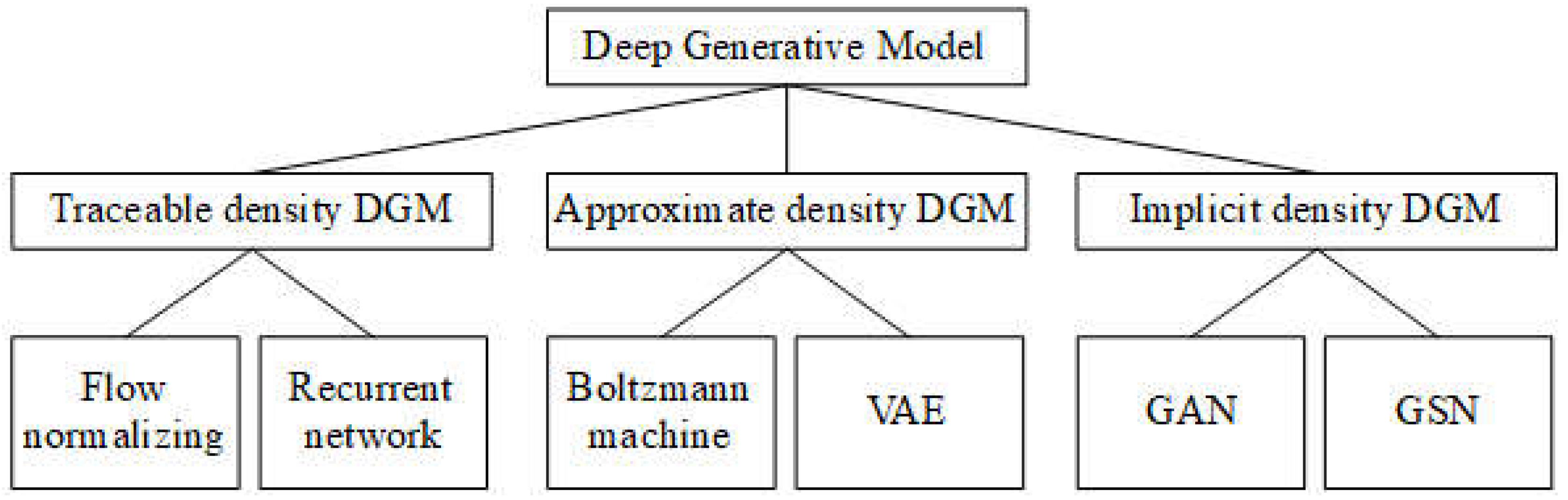
Recall that the two problems of constructing DGM are 1) how to train generator DNN g(z | Φ) and 2) how to qualify such training task which often relates to another optimization task or another training task. The first problem relates to how to establish generator likelihood P(x | Φ, z) which is the probability density function (PDF) of intractable x given tractable data z and this establishment is based on generator DNN g(z | Φ). However, there are some DGMs do not specify explicitly the density function P(x | Φ, z), which is cause of the fact that there are two DGM approaches: 1) DGM specifies explicitly generator PDF P(x | Φ, z) and 2) vice versa. In group of explicit PDF approach, there are two built-in approaches: 1) tractable density DGM specifies explicitly well-known distributions for generator likelihood and 2) approximate density DGM tries to estimate approximately generator PDF P(x | Φ, z) or derive other PDF that is similar to P(x | Φ, z). In general, there are three main approaches for constructing DGM such as tractable density DGM, approximate density DGM, and implicit density DGM which are mentioned in next sections. Following figure depicts taxonomy of DGM (Oussidi & Elhassouny, 2018, p. 7) by Goodfellow.

Figure 1.1. Taxonomy of DGM.

Figure 1.1. Taxonomy of DGM.

Especially, if data is image, there is another categorization way that there are two main approaches: 1) pixel density approach tries to model pixel distribution and 2) block density approach tries to model entire image distribution as any data distribution. In other words, likelihood P(x | Φ, z) is defined based on probabilistic distribution of pixels where x is considered as set of pixels according to pixel density approach. On the other hand, block density approach considers likelihood P(x | Φ, z) is PDF of a block or entire image (unified big block) where x is considered as any arbitrary data. A usual, pixel density approach belongs to tractable density approach of the first categorization.

2. Tractable Density DGM

According to tractable density approach, DGMs specify explicitly generator PDF P(x | Φ, z) with note that PDF is abbreviation of probability density function. Recall that the two problems of constructing DGM are 1) how to train generator DNN g(z | Φ) and 2) how to qualify such training task which often relates to another optimization task or another training task. However, the two problems are merged into the first problem which is to train g(z | Φ) according to normalizing flow technique in which g(z | Φ) is invertible given tractable data z and intractable data x have the same dimension n. Therefore, latent space Z and sample space X are the same with dimension n. As a convention, g^–1(x | Φ) is called inversed generator.

$$\begin{array}{l}\mathit{x}=g\left(\mathit{z}|\mathsf{\Phi }\right)\\ \mathit{z}=g^{-1}\left(\mathit{x}|\mathsf{\Phi }\right)\end{array}$$

(2.1)

Where,

$$\begin{array}{l}\mathit{z}={\left(z_1,z_2,\dots ,z_n\right)}^T,\mathit{x}={\left(x_1,x_2,\dots ,x_n\right)}^T\\ \mathit{x}\in X\subseteq R^n\\ \mathit{z}\in Z\subseteq R^n\\ X=Z\end{array}$$

Note, the subscript “T” denotes transposition operator of vector and matrix in which row vector becomes column vector and vice versa. Because g(z | Φ) is essentially vector-by-vector function whose input and output are vectors, it should have denoted as g(z | Φ), especially, when g(z | Φ) here is bijection. However, it is still denoted g(z | Φ) for convenience. Therefore, the first-order derivative of vector-by-vector function g(z | Φ) here is Jacobian matrix but is stilled called gradient. Note, in mathematical, the first-order derivative of scalar-by-vector function is called gradient vector and the first-order derivative of vector-by-vector function is called Jacobian matrix.

As a result, normalizing flow (NL) technique focuses on maximizing intractable PDF P(x) now called sample PDF or sample likelihood rather than maximizing generator likelihood P(x | Φ, z) because P(x) is now proportional to tractable PDF P(z) and P(x) is stronger than P(x | Φ, z). When P(x) has generator parameter Φ, it is denoted as P(x | Φ). According to applied statistics literature, sample likelihood P(x | Φ) is determined based on tractable PDF P(z) and generator g(z | Φ) as follows (Ruthotto & Haber, 2021, p. 7):

$$P\left(\mathit{x}|\mathsf{\Phi }\right)=P\left(\mathit{z}\right)\left|{\nabla }_{\mathit{x}}{g}^{-1}\left(\mathit{x}|\mathsf{\Phi }\right)\right|=P\left(g^{-1}\left(\mathit{x}|\mathsf{\Phi }\right)\right)\left|{\nabla }_{\mathit{x}}{g}^{-1}\left(\mathit{x}|\mathsf{\Phi }\right)\right|$$

(2.2)

Where |.| or det(.) denotes determinant of square matrix with note that the gradient ∇_xg^–1(x | Φ) of the inverse g^–1(x | Φ) is Jacobian matrix which is the first-order derivative of g^–1(x | Φ) with regard to x. As a convention, ∇_xg^–1(x | Φ) is called inversed gradient because ∇_xg^–1(x | Φ) is the first-order derivative of inversed generator g^–1(x | Φ) with regard to x.

$${\nabla }_{\mathit{x}}{g}^{-1}\left(\mathit{x}|\mathsf{\Phi }\right)=\frac{d{g}^{-1}\left(\mathit{x}|\mathsf{\Phi }\right)}{d\mathit{x}}$$

The equation of sample likelihood P(x | Φ) is much more definite than the integral formulation of P(x) as aforementioned

$$P\left(\mathit{x}\right)=\underset{\mathit{z}}{\int }P\left(\mathit{x}|\mathsf{\Phi },\mathit{z}\right)P\left(\mathit{z}\right)d\mathit{z}$$

It is explained from the equation of sample likelihood P(x | Φ) that given source and target with a function from source to target, target distribution is calculated by multiplying source distribution with determinant of gradient of inversed function.

$$P\left(\mathit{x}|\mathsf{\Phi }\right)=P\left(g^{-1}\left(\mathit{x}|\mathsf{\Phi }\right)\right)\left|{\nabla }_{\mathit{x}}{g}^{-1}\left(\mathit{x}|\mathsf{\Phi }\right)\right|$$

For optimization, P(z) is assumed to follow standard normal distribution with mean 0 and variance 1:

$$P\left(\mathit{z}\right)={\left(2\pi \right)}^{-\frac{n}{2}}\mathrm{e}\mathrm{x}\mathrm{p}\left(-\frac{1}{2}{‖\mathit{z}‖}^2\right)$$

Such that:

$$P\left(\mathit{x}|\mathsf{\Phi }\right)={\left(2\pi \right)}^{-\frac{n}{2}}\mathrm{e}\mathrm{x}\mathrm{p}\left(-\frac{1}{2}{‖g^{-1}\left(\mathit{x}|\mathsf{\Phi }\right)‖}^2\right)\left|{\nabla }_{\mathit{x}}{g}^{-1}\left(\mathit{x}|\mathsf{\Phi }\right)\right|$$

Where notation ||.|| denotes norm of vector. Exactly, P(z) follows standard normal distribution with mean vector 0 and identity covariance matrix I. Sample log-likelihood is derived by taking natural logarithm of sample likelihood:

$$\log P\left(\mathit{x}|\mathsf{\Phi }\right)=-\frac{n}{2}\log 2\pi -\frac{1}{2}{‖g^{-1}\left(\mathit{x}|\mathsf{\Phi }\right)‖}^2+\log \left|{\nabla }_{\mathit{x}}{g}^{-1}\left(\mathit{x}|\mathsf{\Phi }\right)\right|$$

NL aims to maximize sample log-likelihood so as to estimate generator parameter Φ:

$${\mathsf{\Phi }}^{*}=\underset{\mathsf{\Phi }}{\mathrm{armax}}\log P\left(\mathit{x}|\mathsf{\Phi }\right)$$

Stochastic gradient descent (SGD) method is used to estimate Φ by iterative process to update successively Φ at every iteration as follows:

$$\mathsf{\Phi }=\mathsf{\Phi }+\gamma \nabla \log P\left(\mathit{x}|\mathsf{\Phi }\right)$$

Where ∇logP(x | Φ) which is called sample log-likelihood gradient is gradient of sample log-likelihood logP(x | Φ) and γ (0 < γ ≤ 1) is learning rate. Note that SGD, which is an iterative process, pushes candidate solution at each iteration along the direction which is opposite to gradient of target function for minimization or has the same direction to gradient of target function for maximization with note that the step length is represented by learning rate. Given epoch of size N is denoted as D = (x⁽¹⁾, x⁽²⁾,…, x^(N)), the estimation equation of Φ is extended exactly as epoch estimation at every iteration of SGD:

$${\mathsf{\Phi }}^{\left(k+1\right)}={\mathsf{\Phi }}^{\left(k\right)}+\gamma \nabla \frac{1}{N}{\displaystyle \sum _{i=1}^N}\log P\left({\mathit{x}}^{\left(i\right)}|{\mathsf{\Phi }}^{\left(k\right)}\right)$$

It is necessary to determine sample log-likelihood gradient ∇logP(x | Φ) with regard to parameter Φ. Due to (Nguyen, Matrix Analysis and Calculus, 2015, pp. 45-46):

$$\begin{array}{l}\frac{d\log \left(\left|{\nabla }_{\mathit{x}}{g}^{-1}\left(\mathit{x}|\mathsf{\Phi }\right)\right|\right)}{d\mathsf{\Phi }}=\frac{d\log \left(\left|{\nabla }_{\mathit{x}}{g}^{-1}\left(\mathit{x}|\mathsf{\Phi }\right)\right|\right)}{d{\nabla }_{\mathit{x}}{g}^{-1}\left(\mathit{x}|\mathsf{\Phi }\right)}\frac{d{\nabla }_{\mathit{x}}{g}^{-1}\left(\mathit{x}|\mathsf{\Phi }\right)}{d\mathsf{\Phi }}\\ =\frac{d\left|{\nabla }_{\mathit{x}}{g}^{-1}\left(\mathit{x}|\mathsf{\Phi }\right)\right|}{d{\nabla }_{\mathit{x}}{g}^{-1}\left(\mathit{x}|\mathsf{\Phi }\right)}\frac{1}{\left|{\nabla }_{\mathit{x}}{g}^{-1}\left(\mathit{x}|\mathsf{\Phi }\right)\right|}\frac{d{\nabla }_{\mathit{x}}{g}^{-1}\left(\mathit{x}|\mathsf{\Phi }\right)}{d\mathsf{\Phi }}\\ =\frac{\left|{\nabla }_{\mathit{x}}{g}^{-1}\left(\mathit{x}|\mathsf{\Phi }\right)\right|{\left({\nabla }_{\mathit{x}}{g}^{-1}\left(\mathit{x}|\mathsf{\Phi }\right)\right)}^{-1}}{\left|{\nabla }_{\mathit{x}}{g}^{-1}\left(\mathit{x}|\mathsf{\Phi }\right)\right|}\frac{d{\nabla }_{\mathit{x}}{g}^{-1}\left(\mathit{x}|\mathsf{\Phi }\right)}{d\mathsf{\Phi }}\\ ={\left({\nabla }_{\mathit{x}}{g}^{-1}\left(\mathit{x}|\mathsf{\Phi }\right)\right)}^{-1}\frac{d{\nabla }_{\mathit{x}}{g}^{-1}\left(\mathit{x}|\mathsf{\Phi }\right)}{d\mathsf{\Phi }}\end{array}$$

And

$$\frac{d\frac{1}{2}{‖g^{-1}\left(\mathit{x}|\mathsf{\Phi }\right)‖}^2}{d\mathsf{\Phi }}=g^{-1}\left(\mathit{x}|\mathsf{\Phi }\right){\nabla }_{\mathit{x}}{g}^{-1}\left(\mathit{x}|\mathsf{\Phi }\right)$$

We have following equation to calculate log-likelihood gradient ∇logP(x | Φ):

$$\nabla \log P\left(\mathit{x}|\mathsf{\Phi }\right)=\frac{d\log P\left(\mathit{x}|\mathsf{\Phi }\right)}{d\mathsf{\Phi }}={\left({\nabla }_{\mathit{x}}{g}^{-1}\left(\mathit{x}|\mathsf{\Phi }\right)\right)}^{-1}\frac{d{\nabla }_{\mathit{x}}{g}^{-1}\left(\mathit{x}|\mathsf{\Phi }\right)}{d\mathsf{\Phi }}-g^{-1}\left(\mathit{x}|\mathsf{\Phi }\right){\nabla }_{\mathit{x}}{g}^{-1}\left(\mathit{x}|\mathsf{\Phi }\right)$$

The notation (∇_xg^–1(x | Φ))^–1 denotes inverse of matrix ∇_xg^–1(x | Φ). Because ∇_xg^–1(x | Φ) called Jacobian matrix is a square matrix, the derivative d∇_xg^–1(x | Φ) / dΦ is determined by taking first-order derivative for every element of ∇_xg^–1(x | Φ) with regard to Φ, which produces a tensor. Therefore, d∇_xg^–1(x | Φ) / dΦ is the second-order derivative of inversed generator g^–1(x | Φ) with regard to x and Φ. Let

$${\nabla }_{\mathsf{\Phi }}{\nabla }_{\mathit{x}}{g}^{-1}\left(\mathit{x}|\mathsf{\Phi }\right)=\frac{d{\nabla }_{\mathit{x}}{g}^{-1}\left(\mathit{x}|\mathsf{\Phi }\right)}{d\mathsf{\Phi }}$$

It is possible to calculate this second-order derivative if inversed gradient ∇_xg^–1(x | Φ) is determined. Log-likelihood gradient ∇logP(x | Φ) is rewritten:

$$\nabla \log P\left(\mathit{x}|\mathsf{\Phi }\right)={\left({\nabla }_{\mathit{x}}{g}^{-1}\left(\mathit{x}|\mathsf{\Phi }\right)\right)}^{-1}{\nabla }_{\mathsf{\Phi }}{\nabla }_{\mathit{x}}{g}^{-1}\left(\mathit{x}|\mathsf{\Phi }\right)-g^{-1}\left(\mathit{x}|\mathsf{\Phi }\right){\nabla }_{\mathit{x}}{g}^{-1}\left(\mathit{x}|\mathsf{\Phi }\right)$$

(2.3)

Where:

$$\begin{gathered} {\nabla }_{\mathit{x}}{g}^{-1}\left(\mathit{x}|\mathsf{\Phi }\right)=\frac{d{g}^{-1}\left(\mathit{x}|\mathsf{\Phi }\right)}{d\mathit{x}} \\ {\nabla }_{\mathsf{\Phi }}{\nabla }_{\mathit{x}}{g}^{-1}\left(\mathit{x}|\mathsf{\Phi }\right)=\frac{d{\nabla }_{\mathit{x}}{g}^{-1}\left(\mathit{x}|\mathsf{\Phi }\right)}{d\mathsf{\Phi }} \end{gathered}$$

According to traditional neural network, let φ_i be the i^th row vector of matrix Φ, then generator g(x | φ) is linear composition as follows:

$$g\left(\mathit{z}|\phi \right)=a\left({\phi }_i^T\mathit{z}+{\delta }_i\right)=x_i$$

Where δ_i is the i^th bias parameter associated with each x_i. Note, x_i is the i^th elemental variable in x whereas activation a(.) is invertible, whose inverse is a^–1(.). In traditional neural network, x_i represents a neuron or unit. Due to:

$$a^{-1}\left(x_i\right)={\phi }_i^T\mathit{z}+{\delta }_i={\displaystyle \sum _{t=1}^n}{\phi }_{it}{z}_t+{\delta }_i={\phi }_{ij}{z}_j+{\displaystyle \sum _{t=1,t\ne j}^n}{\phi }_{it}{z}_t+{\delta }_i$$

When φ_i = (φ_i1, φ_i2,…, φ_in)^T and z = (z₁, z₂,…, z_n)^T, without loss of generality, given φ_ij and z_j are the j^th elements of φ_i and z, respectively we have fine-tuned inversed generator g^–1(x_i | φ_ij):

$$g^{-1}\left(x_i|{\phi }_{ij}\right)=z_j=\frac{a^{-1}\left(x_i\right)-b_{ij}-{\delta }_i}{{\phi }_{ij}}$$

Where,

$$b_{ij}={\displaystyle \sum _{t=1,t\ne j}^n}{\phi }_{it}{z}_t$$

It is easy to calculate the inversed gradient:

$${\nabla }_{x_i}{g}^{-1}\left(x_i|{\phi }_{ij}\right)=\frac{d\left(a^{-1}\left(x_i\right)-b_{ij}-{\delta }_i\right)/d{x}_i}{{\phi }_{ij}}=\frac{{\left(a^{-1}\left(x_i\right)\right)}^{\prime }}{{\phi }_{ij}}$$

Where a^–1(x_i) is the first-order derivative of a^–1(.) at x_i. The second-order derivative ${\nabla }_{{\phi }_{ij}}{\nabla }_{x_i}{g}^{-1}\left(x_i|{\phi }_{ij}\right)$ is determined as follows:

$${\nabla }_{{\phi }_{ij}}{\nabla }_{x_i}{g}^{-1}\left(x_i|{\phi }_{ij}\right)=\frac{d{\nabla }_{x_i}{g}^{-1}\left(x_i|{\phi }_{ij}\right)}{d{\phi }_{ij}}=-\frac{{\left(a^{-1}\left(x_i\right)\right)}^{\prime }}{{\phi }_{ij}^2}$$

Log-likelihood gradient with regard to φ_ij is fine-tuned as ∇logP(x_i | φ_ij) is expended again:

$$\begin{array}{l}\nabla \log P\left(x_i|{\phi }_{ij}\right)=-\frac{{\phi }_{ij}}{{\left(a^{-1}\left(x_i\right)\right)}^{\prime }}\frac{{\left(a^{-1}\left(x_i\right)\right)}^{\prime }}{{\phi }_{ij}^2}-\frac{a^{-1}\left(x_i\right)}{{\phi }_{ij}}\frac{{\left(a^{-1}\left(x_i\right)\right)}^{\prime }}{{\phi }_{ij}}\\ =-\frac{1}{{\phi }_{ij}}-\frac{a^{-1}\left(x_i\right){\left(a^{-1}\left(x_i\right)\right)}^{\prime }}{{\phi }_{ij}^2}=-\frac{{\phi }_{ij}+a^{-1}\left(x_i\right){\left(a^{-1}\left(x_i\right)\right)}^{\prime }}{{\phi }_{ij}^2}\end{array}$$

Because δ_i is the i^th bias parameter, the second-order derivative ${\nabla }_{{\delta }_i}{\nabla }_{x_i}{g}^{-1}\left(x_i|{\phi }_{ij}\right)$ is determined as follows:

$${\nabla }_{{\delta }_i}{\nabla }_{x_i}{g}^{-1}\left(x_i|{\delta }_i\right)=\frac{d{\nabla }_{x_i}{g}^{-1}\left(x_i|{\delta }_i\right)}{d{\delta }_i}=0$$

Where,

$$\begin{gathered} {\nabla }_{x_i}{g}^{-1}\left(x_i|{\delta }_i\right)=\frac{d\left(a^{-1}\left(x_i\right)-b_{ij}-{\delta }_i\right)/d{x}_i}{{\phi }_{ij}}=\frac{{\left(a^{-1}\left(x_i\right)\right)}^{\prime }}{{\phi }_{ij}} \\ {g}^{-1}\left(x_i|{\delta }_i\right)=z_j=\frac{a^{-1}\left(x_i\right)-b_{ij}-{\delta }_i}{{\phi }_{ij}} \end{gathered}$$

Log-likelihood gradient with regard to δ_i is fine-tuned as ∇logP(x_i | δ_i) is expended again:

$$\nabla \log P\left(x_i|{\delta }_i\right)=-\frac{{\phi }_{ij}}{{\left(a^{-1}\left(x_i\right)\right)}^{\prime }}0-\frac{a^{-1}\left(x_i\right)}{{\phi }_{ij}}\frac{{\left(a^{-1}\left(x_i\right)\right)}^{\prime }}{{\phi }_{ij}}=-\frac{a^{-1}\left(x_i\right){\left(a^{-1}\left(x_i\right)\right)}^{\prime }}{{\phi }_{ij}^2}$$

In general, log-likelihood gradient ∇logP(x_i | φ_ij, δ_i) is specified as follows:

$$\begin{array}{l}\nabla \log P\left(x_i|{\phi }_{ij}\right)=-\frac{1}{{\phi }_{ij}}\left(1+\frac{a^{-1}\left(x_i\right){\left(a^{-1}\left(x_i\right)\right)}^{\prime }}{{\phi }_{ij}}\right),\forall i,j\\ \nabla \log P\left(x_i|{\delta }_i\right)=-\frac{a^{-1}\left(x_i\right){\left(a^{-1}\left(x_i\right)\right)}^{\prime }}{{\phi }_{ij}^2},\forall i\end{array}$$

(2.4)

Where a(.) and a^–1(.) are invertible activation function and its inverse and,

$$\begin{array}{l}{x}_i\in \mathit{x}={\left(x_1,x_2,\dots ,x_n\right)}^T\\ {\phi }_{ij}\in {\phi }_i={\left({\phi }_{i1},{\phi }_{i2},\dots ,{\phi }_{in}\right)}^T\\ {\phi }_i\in \mathsf{\Phi }\\ x_i=a\left({\phi }_i^T\mathit{z}+{\delta }_i\right)\end{array}$$

SGD estimation is fine-tuned as follows:

$$\begin{gathered} {\phi }_{ij}={\phi }_{ij}+\gamma \nabla \log P\left(x_i|{\phi }_{ij}\right)={\phi }_{ij}-\gamma \frac{1}{{\phi }_{ij}}\left(1+\frac{a^{-1}\left(x_i\right){\left(a^{-1}\left(x_i\right)\right)}^{\prime }}{{\phi }_{ij}}\right),\forall i,j \\ {\delta }_i={\delta }_i+\gamma \nabla \log P\left(x_i|{\delta }_i\right)={\delta }_i-\gamma \frac{a^{-1}\left(x_i\right){\left(a^{-1}\left(x_i\right)\right)}^{\prime }}{{\phi }_{ij}^2},\forall i \end{gathered}$$

Given epoch of size N is denoted as D = (x⁽¹⁾, x⁽²⁾,…, x^(N)), the estimation equation of φ_ij and δ_i is extended exactly as epoch estimation at every u^th iteration of SGD with regard to log-likelihood gradient ∇logP(x_i | φ_ij, δ_i).

$$\begin{array}{l}{\phi }_{ij}^{\left(u+1\right)}={\phi }_{ij}^{\left(u\right)}+\gamma \frac{1}{N}\nabla {\displaystyle \sum _{v=1}^N}\log P\left(x_i^{\left(v\right)}|{\phi }_{ij}^{\left(u\right)}\right)\\ ={\phi }_{ij}^{\left(u\right)}-\gamma \frac{1}{{\phi }_{ij}^{\left(u\right)}}\left(1+\frac{1}{N{\phi }_{ij}^{\left(u\right)}}{\displaystyle \sum _{v=1}^N}{a}^{-1}\left(x_i^{\left(v\right)}\right){\left(a^{-1}\left(x_i^{\left(v\right)}\right)\right)}^{\prime }\right),\forall i,j\\ {\delta }_i^{\left(u+1\right)}={\delta }_i^{\left(u\right)}+\gamma \frac{1}{N}\nabla {\displaystyle \sum _{v=1}^N}\log P\left(x_i^{\left(v\right)}|{\delta }_i^{\left(u\right)}\right)\\ ={\delta }_i^{\left(u\right)}-\gamma \frac{1}{N{\left({\phi }_{ij}^{\left(u\right)}\right)}^2}{\displaystyle \sum _{v=1}^N}{a}^{-1}\left(x_i^{\left(v\right)}\right){\left(a^{-1}\left(x_i^{\left(v\right)}\right)\right)}^{\prime },\forall i\end{array}$$

Where x_i^(v) is the i^th element of x^(v) in epoch. As a result, NL trained with SGD is specified as follows:

Initialize all φ_ij, δ_i and set u = 0.

Repeat

Sampling epoch X = (x⁽¹⁾, x⁽²⁾,…, x^(N)) or receiving epoch X from big data / data stream.

$$\begin{gathered} {\phi }_{ij}^{\left(u+1\right)}={\phi }_{ij}^{\left(u\right)}-\gamma \frac{1}{{\phi }_{ij}^{\left(u\right)}}\left(1+\frac{1}{N{\phi }_{ij}^{\left(u\right)}}{\displaystyle \sum _{v=1}^N}{a}^{-1}\left(x_i^{\left(v\right)}\right){\left(a^{-1}\left(x_i^{\left(v\right)}\right)\right)}^{\prime }\right),\forall i,j \\ {\delta }_i^{\left(u+1\right)}={\delta }_i^{\left(u\right)}-\gamma \frac{1}{N{\left({\phi }_{ij}^{\left(u\right)}\right)}^2}{\displaystyle \sum _{v=1}^N}{a}^{-1}\left(x_i^{\left(v\right)}\right){\left(a^{-1}\left(x_i^{\left(v\right)}\right)\right)}^{\prime },\forall i \end{gathered}$$

Increase u = u + 1.

Until some terminating conditions are met.

Note, a terminating condition is customized, for example, parameters φ_ij and δ_i are not changed significantly or there is no more coming epoch X. Moreover, the index u indicates time point as well as iteration of SGD. After finite NL is trained, it can generate new data x’ by generator g(z | Φ) = x’ with any z randomized from standard normal distribution with mean 0 and variance 1.

It is interesting that log-likelihood gradient ∇logP(x_i | φ_ij) is determined based on inversed gradient ${\nabla }_{x_i}{g}^{-1}\left(x_i|{\phi }_{ij}\right)$. Therefore, how to estimate generator parameter Φ by SGD estimation focuses on calculating inversed gradient ${\nabla }_{x_i}{g}^{-1}\left(x_i|{\phi }_{ij}\right)$ which is central point of normalizing flow (NL) technique. Moreover, how to calculate ${\nabla }_{x_i}{g}^{-1}\left(x_i|{\phi }_{ij}\right)$ is based on how to determine inversed generator g^–1(x | Φ). In other words, the main problem of NL is how to determine inversed generator g^–1(x | Φ) because it is easy to calculate gradient of function f(x) = g^–1(x | Φ) with regard to x. Especially, when generator g(x | Φ) is implemented by DNN, NL will have some special techniques so that determining its inverse g^–1(x | Φ) is easier. One of these technique is finite normalizing flow (finite NL) in which generator g(x | Φ) is implemented by a DNN having K layers from layer 1 to layer K where layer 0 is input layer with note that each layer is represented by partial generator function f_k (Ruthotto & Haber, 2021, p. 8):

$$g\left(\mathit{z}|\mathsf{\Phi }\right)=f_K\circ f_{K-1}\circ \dots \circ f_2\circ f_1\left(\mathit{z}\right)$$

(2.5)

Note, all layers f_k have the same number of neurons which is the dimension n. Because f_k is essentially vector-by-vector function whose input and output are vectors, it should have denoted as f_k, especially, when f_k here is bijection. However, it is still denoted f_k for convenience. Let z^(k+1) be output of partial generator f_k, we have:

$$\begin{gathered} {\mathit{z}}^{\left(k+1\right)}=f_k\left({\mathit{z}}^{\left(k\right)}\right) \\ \mathit{z}={\mathit{z}}^{\left(1\right)}={\mathit{z}}^{\left(0\right)}=f_0\left({\mathit{z}}^{\left(0\right)}\right)\equiv f_0 \\ \mathit{x}={\mathit{z}}^{\left(K+1\right)}=f_K\left({\mathit{z}}^{\left(K\right)}\right) \end{gathered}$$

Inversed generator g^–1(x | Φ) representing inversed DNN is determined:

$$g^{-1}\left(\mathit{x}|\mathsf{\Phi }\right)=f_1^{-1}\circ f_2^{-1}\circ \dots \circ f_{K-1}^{-1}\circ f_K^{-1}\left(\mathit{x}\right)$$

(2.6)

Each f_k^–1 is called inversed partial generator function which is the inverse of partial generator function f_k. Let x^(k–1) be output of partial generator f_k^–1, we have:

$$\begin{gathered} {\mathit{x}}^{\left(k-1\right)}=f_k^{-1}\left({\mathit{x}}^{\left(k\right)}\right) \\ \mathit{x}={\mathit{x}}^{\left(K+1\right)}={\mathit{x}}^{\left(K\right)}=f_{K+1}^{-1}\left({\mathit{x}}^{\left(K+1\right)}\right)\equiv f_{K+1}^{-1} \\ \mathit{z}={\mathit{x}}^{\left(0\right)}=f_2^{-1}\left({\mathit{x}}^{\left(1\right)}\right) \end{gathered}$$

“Input layer” of “inversed DNN” is f_K+1^–1. The inversed generator DNN may be pseudo in case that only one generator DNN is designed so that inversed generator function f_k^–1 is existent. An interesting result of the design of finite NL is that inversed gradient ∇g^–1(x | Φ) is product of gradients of inversed partial generator f_k^–1.

$$\begin{gathered} {\nabla }_{\mathit{x}}{g}^{-1}\left(\mathit{x}|\mathsf{\Phi }\right)={\displaystyle \prod _{k=1}^K}{\nabla }_{{\mathit{x}}^{\left(k\right)}}{f}_k^{-1}\left({\mathit{x}}^{\left(k\right)}|{\mathsf{\Phi }}^{\left(k\right)}\right) \\ \log \left|{\nabla }_{\mathit{x}}{g}^{-1}\left(\mathit{x}|\mathsf{\Phi }\right)\right|={\displaystyle \sum _{k=1}^K}\left|{\nabla }_{{\mathit{x}}^{\left(k\right)}}{f}_k^{-1}\left({\mathit{x}}^{\left(k\right)}|{\mathsf{\Phi }}^{\left(k\right)}\right)\right| \end{gathered}$$

Where Φ^(k) is parameter of f_k. It is now necessary to determine fine-tuned partial inversed gradient ${\nabla }_{x_i^{\left(k\right)}}{f}_k^{-1}\left(x_i^{\left(k\right)}|{\phi }_{ij}^{\left(k\right)}\right)$ in order to determine fine-tuned partial log-likelihood gradient ∇logP(x_i^(k) | φ_ij^(k)) where x_i^(k) is an elemental variable in x^(k) = (x₁^(k), x₂^(k),…, x_n^(k))^T and φ_ij^(k) is the j^th element in φ_i^(k) = (φ_i1^(k), φ_i2^(k),…, φ_in^(k))^T with note that φ_i^(k) is the i^th row vector of matrix Φ^(k). Moreover, let δ_i^(k) be the ith bias parameter associated with each x_i^(k). Without loss of generality, given φ_j^(k), δ_i^(k), and z_j^(k) along with invertible activation a(.), we have fine-tuned inversed generator g^–1(x_i^(k) | φ_ij^(k), δ_i^(k)).

$$f_k^{-1}\left(x_i^{\left(k\right)}|{\phi }_{ij}^{\left(k\right)}\right)=z_j^{\left(k\right)}=\frac{a^{-1}\left(x_i^{\left(k\right)}\right)-b_{ij}^{\left(k\right)}-{\delta }_i^{\left(k\right)}}{{\phi }_{ij}^{\left(k\right)}}$$

Where,

$$b_{ij}^{\left(k\right)}={\displaystyle \sum _{t=1,t\ne j}^n}{\phi }_{it}^{\left(k\right)}{z}_t^{\left(k\right)}$$

Where z_i^(k) is the i^th elemental variable in z^(k) = (z₁^(k), z₂^(k),…, z_n^(k))^T. By similar way aforementioned, log-likelihood gradient ∇logP(x_i^(k) | φ_ij^(k), δ_i^(k)) is specified as follows:

$$\begin{gathered} \nabla \log P\left(x_i^{\left(k\right)}|{\phi }_{ij}^{\left(k\right)}\right)=-\frac{1}{{\phi }_{ij}^{\left(k\right)}}\left(1+\frac{a^{-1}\left(x_i^{\left(k\right)}\right){\left(a^{-1}\left(x_i^{\left(k\right)}\right)\right)}^{\prime }}{{\phi }_{ij}^{\left(k\right)}}\right),\forall i,j \\ \nabla \log P\left(x_i^{\left(k\right)}|{\delta }_i^{\left(k\right)}\right)=-\frac{a^{-1}\left(x_i^{\left(k\right)}\right){\left(a^{-1}\left(x_i^{\left(k\right)}\right)\right)}^{\prime }}{{\left({\phi }_{ij}^{\left(k\right)}\right)}^2},\forall i \end{gathered}$$

(2.7)

Where a(.) and a^–1(.) are invertible activation function and its inverse and,

$$\begin{array}{l}{x}_i^{\left(k\right)}\in {\mathit{x}}^{\left(k\right)}={\left(x_1^{\left(k\right)},x_2^{\left(k\right)},\dots ,x_n^{\left(k\right)}\right)}^T\\ {\phi }_{ij}^{\left(k\right)}\in {\phi }_i^{\left(k\right)}={\left({\phi }_{i1}^{\left(k\right)},{\phi }_{i2}^{\left(k\right)},\dots ,{\phi }_{in}^{\left(k\right)}\right)}^T\\ {\phi }_i^{\left(k\right)}\in {\mathsf{\Phi }}^{\left(k\right)}\\ x_i^{\left(k\right)}=a\left({\left({\phi }_i^{\left(k\right)}\right)}^T\mathit{z}+{\delta }_i^{\left(k\right)}\right)\end{array}$$

SGD estimation is fine-tuned as follows:

$$\begin{gathered} {\phi }_{ij}^{\left(k\right)}={\phi }_{ij}^{\left(k\right)}+\gamma \nabla \log P\left(x_i^{\left(k\right)}|{\phi }_{ij}^{\left(k\right)}\right)={\phi }_{ij}^{\left(k\right)}-\gamma \frac{1}{{\phi }_{ij}^{\left(k\right)}}\left(1+\frac{a^{-1}\left(x_i^{\left(k\right)}\right){\left(a^{-1}\left(x_i^{\left(k\right)}\right)\right)}^{\prime }}{{\phi }_{ij}^{\left(k\right)}}\right),\forall i,j \\ {\delta }_i^{\left(k\right)}={\delta }_i^{\left(k\right)}+\gamma \nabla \log P\left(x_i^{\left(k\right)}|{\delta }_i^{\left(k\right)}\right)={\delta }_i^{\left(k\right)}-\gamma \frac{a^{-1}\left(x_i^{\left(k\right)}\right){\left(a^{-1}\left(x_i^{\left(k\right)}\right)\right)}^{\prime }}{{\left({\phi }_{ij}^{\left(k\right)}\right)}^2},\forall i \end{gathered}$$

Given epoch of size N is denoted as D = (x⁽¹⁾, x⁽²⁾,…, x^(N)), the estimation equation of φ_ij^(k) and δ_i^(k) is extended exactly as epoch estimation at every u^th iteration of SGD with regard to log-likelihood gradient ∇logP(x_i^(k) | φ_ij^(k), δ_i^(k)):

$$\begin{array}{l}{\left({\phi }_{ij}^{\left(k\right)}\right)}^{\left(u+1\right)}={\left({\phi }_{ij}^{\left(k\right)}\right)}^{\left(u\right)}+\gamma \frac{1}{N}\nabla {\displaystyle \sum _{v=1}^N}\log P\left({\left(x_i^{\left(k\right)}\right)}^{\left(v\right)}|{\left({\phi }_{ij}^{\left(k\right)}\right)}^{\left(u\right)}\right)\\ ={\left({\phi }_{ij}^{\left(k\right)}\right)}^{\left(u\right)}\\ -\gamma \frac{1}{{\left({\phi }_{ij}^{\left(k\right)}\right)}^{\left(u\right)}}\\ \left(1+\frac{1}{N{\left({\phi }_{ij}^{\left(k\right)}\right)}^{\left(u\right)}}{\displaystyle \sum _{v=1}^N}{a}^{-1}\left({\left(x_i^{\left(k\right)}\right)}^{\left(v\right)}\right){\left(a^{-1}\left({\left(x_i^{\left(k\right)}\right)}^{\left(v\right)}\right)\right)}^{\prime }\right),\forall i,j\\ {\left({\delta }_i^{\left(k\right)}\right)}^{\left(u+1\right)}={\left({\delta }_i^{\left(k\right)}\right)}^{\left(u\right)}+\gamma \frac{1}{N}\nabla {\displaystyle \sum _{v=1}^N}\log P\left({\left(x_i^{\left(k\right)}\right)}^{\left(v\right)}|{\left({\delta }_i^{\left(k\right)}\right)}^{\left(u\right)}\right)\\ ={\left({\delta }_i^{\left(k\right)}\right)}^{\left(u\right)}-\gamma \frac{1}{N{\left({\left({\phi }_{ij}^{\left(k\right)}\right)}^{\left(u\right)}\right)}^2}{\displaystyle \sum _{v=1}^N}{a}^{-1}\left({\left(x_i^{\left(k\right)}\right)}^{\left(v\right)}\right){\left(a^{-1}\left({\left(x_i^{\left(k\right)}\right)}^{\left(v\right)}\right)\right)}^{\prime },\forall i\end{array}$$

Where (x_i^(k))^(v) is the i^th element of x^(v) in epoch with regard to inversed generator f_k^–1. As a result, finite NL trained with SGD is specified as follows:

Initialize all φ_ij^(k), δ_i^(k) and set u = 0.

Repeat

Sampling epoch X = (x⁽¹⁾, x⁽²⁾,…, x^(N)) or receiving epoch X from big data / data stream.

$$\begin{array}{l}{\left({\phi }_{ij}^{\left(k\right)}\right)}^{\left(u+1\right)}={\left({\phi }_{ij}^{\left(k\right)}\right)}^{\left(u\right)}\\ -\gamma \frac{1}{{\left({\phi }_{ij}^{\left(k\right)}\right)}^{\left(u\right)}}\\ \left(1+\frac{1}{N{\left({\phi }_{ij}^{\left(k\right)}\right)}^{\left(u\right)}}{\displaystyle \sum _{v=1}^N}{a}^{-1}\left({\left(x_i^{\left(k\right)}\right)}^{\left(v\right)}\right){\left(a^{-1}\left({\left(x_i^{\left(k\right)}\right)}^{\left(v\right)}\right)\right)}^{\prime }\right),\forall i,j\\ {\left({\delta }_i^{\left(k\right)}\right)}^{\left(u+1\right)}={\left({\delta }_i^{\left(k\right)}\right)}^{\left(u\right)}-\gamma \frac{1}{N{\left({\left({\phi }_{ij}^{\left(k\right)}\right)}^{\left(u\right)}\right)}^2}{\displaystyle \sum _{v=1}^N}{a}^{-1}\left({\left(x_i^{\left(k\right)}\right)}^{\left(v\right)}\right){\left(a^{-1}\left({\left(x_i^{\left(k\right)}\right)}^{\left(v\right)}\right)\right)}^{\prime },\forall i\end{array}$$

Increase u = u + 1.

Until some terminating conditions are met.

Note, a terminating condition is customized, for example, parameters φ_ij^(k) and δ_i^(k) are not changed significantly or there is no more coming epoch X. Moreover, the index u indicates time point as well as iteration of SGD. After finite NL is trained, it can generate new data x’ by generator g(z | Φ) = x’ with any z randomized from standard normal distribution with mean 0 and variance 1.

Because it is not easy to calculate inversed gradient ∇_xg^–1(x | Φ) as well as its determinant |∇_xg^–1(x | Φ)| according to finite NL except the decomposition technique above of entire matrix parameter Φ into partial vector parameters φ_i^(k), there is technique called real RVP (Ruthotto & Haber, 2021, p. 9) which defines each layer or partial generator f_k(z^(k)) by special way where z^(k) is split into two parts such as z₁^(k) and z₂^(k) so that:

$$f_k\left({\mathit{z}}^{\left(k\right)}\right)=f_k\left(\begin{array}{c}{\mathit{z}}_1^{\left(k\right)}\\ {\mathit{z}}_2^{\left(k\right)}\end{array}\right)=\left(\begin{array}{c}{\mathit{z}}_1^{\left(k\right)}\\ {\mathit{z}}_2^{\left(k\right)}⨂\mathrm{e}\mathrm{x}\mathrm{p}\left({\mathit{s}}_k\left({\mathit{z}}_1^{\left(k\right)}\right)\right)+{\mathit{t}}_k\left({\mathit{z}}_1^{\left(k\right)}\right)\end{array}\right)$$

(2.8)

Of course, we have:

$$f_k\left({\mathit{z}}^{\left(k\right)}\right)=f_k\left(\begin{array}{c}{\mathit{z}}_1^{\left(k\right)}\\ {\mathit{z}}_2^{\left(k\right)}\end{array}\right)=\left(\begin{array}{c}{\mathit{z}}_1^{\left(k\right)}\\ {\mathit{z}}_2^{\left(k\right)}⨂\mathrm{e}\mathrm{x}\mathrm{p}\left({\mathit{s}}_k\left({\mathit{z}}_1^{\left(k\right)}\right)\right)+{\mathit{t}}_k\left({\mathit{z}}_1^{\left(k\right)}\right)\end{array}\right)=\left(\begin{array}{c}{\mathit{z}}_1^{\left(k+1\right)}\\ {\mathit{z}}_2^{\left(k+1\right)}\end{array}\right)={\mathit{z}}^{\left(k+1\right)}$$

Where s_k and t_k are two neural networks for scaling and translation, whose inputs and outputs have the same dimension. The operator $⨂$ denotes component-wise multiplication of two vectors where every pair of two corresponding elements of the two vectors are multiplied together, for instance, given two arbitrary vectors u = (u₁, u₂,…, u_n)^T and v = (v₁, v₂,…, v_n)^T, we have u$⨂$v = (u₁v₁, u₂v₂,…, u_nv_n)^T. Moreover, the exponential function exp(.) above whose input is vector produces a vector by taking exponential function over every element of input vector. Inversed generator f_k^–1 is specified from generator f_k.

$$f_k^{-1}\left({\mathit{x}}^{\left(k\right)}\right)=f_k^{-1}\left(\begin{array}{c}{\mathit{x}}_1^{\left(k\right)}\\ {\mathit{x}}_2^{\left(k\right)}\end{array}\right)=\left(\begin{array}{c}{\mathit{x}}_1^{\left(k\right)}\\ \left({\mathit{x}}_2^{\left(k\right)}-{\mathit{t}}_k\left({\mathit{x}}_1^{\left(k\right)}\right)\right)⨂\mathrm{e}\mathrm{x}\mathrm{p}\left(-{\mathit{s}}_k\left({\mathit{x}}_1^{\left(k\right)}\right)\right)\end{array}\right)$$

(2.9)

Of course, we have:

$$\begin{array}{l}{f}_k^{-1}\left({\mathit{x}}^{\left(k\right)}\right)=f_k^{-1}\left(\begin{array}{c}{\mathit{x}}_1^{\left(k\right)}\\ {\mathit{x}}_2^{\left(k\right)}\end{array}\right)=\left(\begin{array}{c}{\mathit{x}}_1^{\left(k\right)}\\ \left({\mathit{x}}_2^{\left(k\right)}-{\mathit{t}}_k\left({\mathit{x}}_1^{\left(k\right)}\right)\right)⨂\mathrm{e}\mathrm{x}\mathrm{p}\left(-{\mathit{s}}_k\left({\mathit{x}}_1^{\left(k\right)}\right)\right)\end{array}\right)=\left(\begin{array}{c}{\mathit{x}}_1^{\left(k-1\right)}\\ {\mathit{x}}_2^{\left(k-1\right)}\end{array}\right)\\ ={\mathit{x}}^{\left(k-1\right)}\end{array}$$

Inversed gradient ${\nabla }_{{\mathit{x}}^{\left(k\right)}}{f}_k^{-1}\left({\mathit{x}}^{\left(k\right)}\right)$ is the 2x2 Jacobian matrix determined as follows:

$${\nabla }_{{\mathit{x}}^{\left(k\right)}}{f}_k^{-1}\left({\mathit{x}}^{\left(k\right)}\right)=\left(\begin{array}{cc}1& 0\\ \frac{d\left({\mathit{x}}_2^{\left(k\right)}-{\mathit{t}}_k\left({\mathit{x}}_1^{\left(k\right)}\right)\right)⨂\mathrm{e}\mathrm{x}\mathrm{p}\left(-{\mathit{s}}_k\left({\mathit{x}}_1^{\left(k\right)}\right)\right)}{d{\mathit{x}}_1^{\left(k\right)}}& \mathrm{e}\mathrm{x}\mathrm{p}\left(-{\mathit{s}}_k\left({\mathit{x}}_1^{\left(k\right)}\right)\right)\end{array}\right)$$

It is interesting that taking determinant of inversed gradient ∇_xf_k^–1(x^(k)) becomes simple:

$$\left|{\nabla }_{{\mathit{x}}^{\left(k\right)}}{f}_k^{-1}\left({\mathit{x}}^{\left(k\right)}\right)\right|=\mathrm{e}\mathrm{x}\mathrm{p}\left(-{\mathit{s}}_k\left({\mathit{x}}_1^{\left(k\right)}\right)\right)$$

(2.10)

When this determinant is determined, it is possible to maximize log-likelihood logP(x | Φ) to estimate Φ where Φ here are weights of scaling neural network s_k and translation neural network t_k. Log-likelihood logP(x | Φ) is written:

$$\begin{array}{l}\log P\left(\mathit{x}|\mathsf{\Phi }\right)=-\frac{n}{2}\log 2\pi -\frac{1}{2}{‖g^{-1}\left(\mathit{x}|\mathsf{\Phi }\right)‖}^2+\log \left|{\nabla }_{\mathit{x}}{g}^{-1}\left(\mathit{x}|\mathsf{\Phi }\right)\right|\\ =\frac{n}{2}\log 2\pi -\frac{1}{2}{‖g^{-1}\left(\mathit{x}|\mathsf{\Phi }\right)‖}^2+{\displaystyle \sum _{k=1}^K}\log \left|{\nabla }_{{\mathit{x}}^{\left(k\right)}}{f}_k^{-1}\left({\mathit{x}}^{\left(k\right)}\right)\right|\\ =\frac{n}{2}\log 2\pi -\frac{1}{2}{‖g^{-1}\left(\mathit{x}|\mathsf{\Phi }\right)‖}^2-{\displaystyle \sum _{k=1}^K}{\mathit{s}}_k\left({\mathit{x}}_1^{\left(k\right)}\right)\end{array}$$

Because parameter Φ is now only weights of scaling neural network s_k and translation neural network t_k, maximizing log-likelihood logP(x | Φ) is now to optimize (train) s_k and t_k by some algorithms like backpropagation algorithm.

$$\begin{gathered} {\left({\mathsf{\Phi }}_{\mathit{s}}^{\left(k\right)}\right)}^{*}=\underset{{\mathsf{\Phi }}_s^{\left(k\right)}}{\mathrm{optimize}}{\mathit{s}}_k\left({\mathit{x}}_1^{\left(k\right)}|{\mathsf{\Phi }}_{\mathit{s}}^{\left(k\right)}\right) \\ {\left({\mathsf{\Phi }}_{\mathit{t}}^{\left(k\right)}\right)}^{*}=\underset{{\mathsf{\Phi }}_t^{\left(k\right)}}{\mathrm{optimize}}{\mathit{t}}_k\left({\mathit{x}}_1^{\left(k\right)}|{\mathsf{\Phi }}_{\mathit{t}}^{\left(k\right)}\right) \end{gathered}$$

Beside finite NL there is another NL technique called continuous NL but it is not mentioned here because continuous NL is relevant to hazard problem of differential equation which is not main subject of DNN.

Recall that there are three main approaches for constructing DGM such as tractable density DGM, approximate density DGM, and implicit density DGM. However, if data is image, there is another categorization way that there are two main approaches: 1) pixel density approach tries to model pixel distribution and 2) block density approach tries to model entire image distribution as any data distribution. In other words, likelihood P(x | Φ, z) is defined based on probabilistic distribution of pixels where x is considered as set of pixels according to pixel density approach. On the other hand, block density approach considers likelihood P(x | Φ, z) is PDF of a block or entire image (unified big block) where x is considered as any arbitrary data. For instance, NL belongs to both tractable density DGM and block density approach. It is interesting that pixel density approach also belongs to tractable density approach because its PDF is defined obviously. Moreover, pixel density approach merges the two problems of training generator g(z | Φ) and qualifying such training task into the first problem which is to train g(z | Φ) by learning sample PDF P(x) because P(x) or P(x | Φ) now replaces P(x | Φ, z).

Shortly, pixel density (PD) approach defines P(x) as product of all pixel distribution. Concretely, let x = (x₁, x₂,…, $x_{n^2}$)^T denote an image whose every i^th pixel is represented by elemental variable x_i and P(x) called image PDF is defined according to joint probability rule as follows:

$$P\left(\mathit{x}\right)={\displaystyle \prod _{i=1}^{n^2}}P\left(x_i|x_{i-1},x_{i-2},\dots ,x_1\right)$$

(2.11)

Where n implies image width with suppose that image width and image height are equal for convenience, and

$$P\left(x_1|x_0\right)=P\left(x_1\right)$$

In other words, image PDF P(x) is product of all conditional PDFs P(x_i | x_i–1, x_i–2,…, x₁) where every P(x_i | x_i–1, x_i–2,…, x₁) is called conditional pixel PDF or pixel PDF in short. There is neither tractable data z nor explicit generator g(z | Φ) for generating new data in PD because generation task is based on the entire PDF P(x). For instance, without loss of generality, if we randomize k first pixels x₁, x₂,…, x_k, we can generate n²–k remaining pixels by the recurrent process: determining P(x_k+1 | x_k, x_k–1,…, x₁) based on x₁ to x_k, generating x_k+1 according to P(x_k+1 | x_k, x_k–1,…, x₁) and determining P(x_k+2 | x_k+1, x_k,…, x₁) based on x₁ to x_k+1, generating x_k+2 according to P(x_k+2 | x_k+1, x_k,…, x₁) and determining P(x_k+3 | x_k+2, x_k+1,…, x₁) based on x₁ to x_k+2,…, generating $x_{n^2-1}$ according to P($x_{n^2-1}$ | $x_{n^2-2}$, $x_{n^2-3}$,…, x₁) and determining P($x_{n^2}$ | $x_{n^2-1}$, $x_{n^2-2}$,…, x₁) based on x₁ to $x_{n^2-1}$, generating the last $x_{n^2}$ according to P($x_{n^2}$ | $x_{n^2-1}$, $x_{n^2-2}$,…, x₁). By another viewpoint, the joint probability of n²–k remaining pixels denoted P(x_k, x_k+1,…, $x_{n^2}$) is determined and then, n²–k remaining pixels are generated according to this joint probability. Indeed, the joint probability P(x_k, x_k+1,…, $x_{n^2}$) of n²–k remaining pixels is totally determined when P(x) and k probabilities P(x_i | x_i–1, x_i–2,…, x₁) are determined where i is from 1 to k.

$$P\left(x_{k+1},x_{k+2},\dots ,x_{n^2}\right)={\displaystyle \prod _{i=k+1}^{n^2}}P\left(x_i|x_{i-1},x_{i-2},\dots ,x_1\right)=\frac{P\left(\mathit{x}\right)}{{\displaystyle \prod _{i=1}^k}P\left(x_i|x_{i-1},x_{i-2},\dots ,x_1\right)}$$

Because there are a large number of pixels in a large image which produces a large number of pixel PDFs as well as every pixel PDF P(x_i | x_i–1, x_i–2,…, x₁) of a given pixel x_i is itself also complicated with a lot of its previous pixels x_i–1, x_i–2,…, x₁, there are many techniques proposed to PD in order to decrease complexity and increase computation effectiveness. Anyhow, the equation of image PDF P(x) above is important one in theory. One of PD techniques is to apply long short-term memory (LSTM) (Theis & Bethge, 2015) into modeling and learning sample PDF P(x).

The default artificial neural network is feedforward neural network where data is fed to input layer which, in turn, is evaluated and passed across hidden layers to output layer in one-way direction, finally. However, there is an extension of neural network, which is called recurrent neural work (RNN), where an output can be turned back in order to feed on network as input. In other words, RNN has circle, which allow that output can become input. For convenience and easy explanation, given T time points t = 1, 2,…, T, current state of a RNN at time point t is represented by three layers such as input layer x_t, hidden layer h_t, and output layer o_t without loss of generality with note that h_t can represent many hidden layers when RNN is a DNN too. Obviously, RNN is an extension of neural network because every triple (x_t, h_t, o_t) is, essentially, a feedforward neural network, even a DNN. Hidden layer h_t as well as output layer o_t at current state t is calculated based on both current input layer x_t and previous hidden layer h_t–1 of previous state at time point t–1. Without loss of generality, input layer, hidden layer, and output layer are considered as input neuron, hidden neuron, and output neuron for convenience (Wikipedia, Recurrent neural network, 2005).

$$\begin{array}{l}{\mathit{h}}_t={\sigma }_{\mathit{h}}\left({\mathit{W}}_{\mathit{h}}{\mathit{x}}_t+{\mathit{U}}_{\mathit{h}}{\mathit{h}}_{t-1}+{\mathit{b}}_{\mathit{h}}\right)\\ {\mathit{o}}_t={\sigma }_{\mathit{o}}\left({\mathit{W}}_{\mathit{o}}{\mathit{h}}_t+{\mathit{b}}_{\mathit{o}}\right)\end{array}$$

(2.12)

Where W_h is weight matrix of current hidden neuron h_t regarding current input neuron x_t, U_h is weight matrix of current hidden neuron h_t regarding previous hidden neuron h_t–1, and b_h is bias vector of current hidden neuron h_t whereas W_o is weight matrix of current output neuron o_t regarding current hidden neuron h_t and b_o is bias vector of current output neuron o_t. Moreover, σ_h(.) and σ_o(.) are activation functions of h_t and o_t, respectively with note that σ_h(.) and σ_o(.) are vector-by-vector functions. Backpropagation algorithm can be applied into learning RNN as usual. It is interesting that structure of RNN defined by the triple (x_t, h_t, o_t) is not changed but its parameters W_h, U_h, b_h, W_o, and b_o are changed by backpropagation algorithm when RNN is learned. Of course, values of the triple (x_t, h_t, o_t) are changed over time points. Note, W_h, U_h, and W_o are matrix parameters and b_h and b_o are vector parameters whereas x_t, h_t, and o_t are vector variables.

Long short-term memory (LSTM) is an extension of RNN, which implies that RNN is used to implement short-term memory so that the short-term memory can last for a longer time through T time points t = 1, 2,…, T built in RNN. Consequently, the short-term memory is represented by a so-called cell associated with three gates such as input gate, forget gate, and output gate. Cell represents information piece stored in memory at current time (Wikipedia, 2007). Input gate controls which new information to be put to cell, forget gate decides which information to be discarded, and output gate controls which information to be sent to next state (Wikipedia, 2007). As a convention, the cell at current state t is represented by the pair (c_t, h_t) whereas input gate, forget gate, and output gate are represented by vector variables i_t, f_t, and o_t, respectively. Note, let g_t and c_t be cell input activation variable and cell state variable where cell input activation variable g_t represents the activated input part of a cell, which is the important input part being different from the forgotten part, whereas cell state variable c_t represents real information stored in cell which is, exactly, the short memory at current state. In literature, g_t is also called cell gate. Some LSTM variants merge g_t and c_t into the same cell state variable. Although output gate o_t represents which information to be sent to next state, it is consolidated with current cell memory c_t in order to produce the real output information h_t which represents bright and clear-cut memory. In other words, given cell (c_t, h_t), then c_t represents the real information stored in memory and h_t represents the clear-cut memory which displays brightly at the outside for next state. It is possible to consider that c_t is evaluated value of cell t and h_t is predictive value of cell t. Following equations specify LSTM based on specification of RNN (Wikipedia, 2007), which indicates how to calculate cell and gates.

$$\begin{array}{l}{\mathit{i}}_t={\sigma }_{\mathit{i}}\left({\mathit{W}}_{\mathit{i}}{\mathit{x}}_t+{\mathit{U}}_{\mathit{i}}{\mathit{h}}_{t-1}+{\mathit{b}}_{\mathit{i}}\right)\\ {\mathit{f}}_t={\sigma }_{\mathit{f}}\left({\mathit{W}}_{\mathit{f}}{\mathit{x}}_t+{\mathit{U}}_{\mathit{f}}{\mathit{h}}_{t-1}+{\mathit{b}}_{\mathit{f}}\right)\\ {\mathit{o}}_t={\sigma }_{\mathit{o}}\left({\mathit{W}}_{\mathit{o}}{\mathit{x}}_t+{\mathit{U}}_{\mathit{o}}{\mathit{h}}_{t-1}+{\mathit{b}}_{\mathit{o}}\right)\\ {\mathit{g}}_t={\sigma }_{\mathit{g}}\left({\mathit{W}}_{\mathit{g}}{\mathit{x}}_t+{\mathit{U}}_{\mathit{g}}{\mathit{h}}_{t-1}+{\mathit{b}}_{\mathit{g}}\right)\\ {\mathit{c}}_t={\mathit{f}}_t⨂{\mathit{c}}_{t-1}+{\mathit{i}}_t⨂{\mathit{g}}_t\\ {\mathit{h}}_t={\mathit{o}}_t⨂{\sigma }_{\mathit{h}}\left({\mathit{c}}_t\right)\end{array}$$

(2.13)

Note, weight matrix W_i, weight matrix U_i, and bias vector b_i are parameters of input gate i_t. Weight matrix W_f, weight matrix U_f, and bias vector b_f are parameters of forget gate f_t. Weight matrix W_o, weight matrix U_o, and bias vector b_o are parameters of output gate o_t. Weight matrix W_g, weight matrix U_g, and bias vector b_g are parameters of cell gate g_t. Vector variables i_t, f_t, and o_t are often in range [0, 1] whereas vector variables c_t and h_t are often in range [–1, 1]. Activation functions σ_i(.), σ_f(.), and σ_o(.) are often sigmoid (logistic) functions whereas activation functions σ_g(.) and σ_h(.) are hyperbolic tangent functions. The operator $⨂$ denotes component-wise multiplication of two vectors where every pair of two corresponding elements of the two vectors are multiplied together, for instance, given two arbitrary vectors u = (u₁, u₂,…, u_n)^T and v = (v₁, v₂,…, v_n)^T, we have u$⨂$v = (u₁v₁, u₂v₂,…, u_nv_n)^T. Note, backpropagation algorithm can be applied into learning LSTM as usual.

By applying LSTM into pixel density (PD) approach for modeling DGM, each pixel x_i is represented by cell c_i when pixel index i is considered as time point t. Because each cell c_i is dependent on its one right previous cell c_i–1 whereas conditional pixel PDF P(x_i | x_i–1, x_i–2,…, x₁) of pixel x_i is dependent on i–1 previous pixelsx_i–1, x_i–2,…, x₁, Markov property is applied so that conditional pixel PDF of pixel x_i depends on only one previous pixel x_i–1.

$$P\left({\mathit{x}}_i|{\mathit{x}}_{i-1},{\mathit{x}}_{i-2},\dots ,{\mathit{x}}_1\right)=P\left({\mathit{x}}_i|{\mathit{x}}_{i-1}\right)$$

It is now possible to apply LSTM to model PD by matching each pixel x_i with each cell c_i so that cell c_i is considered as evaluated value of pixel x_i as well as each h_i is predictive value of pixel x_i. Because image is two-dimension array, each pixel x_ij or each cell c_ij is indexed by two indices i and j following image height and image width. The event that cell c_ij or c_i,j indexed by two indices i and j makes LSTM extended into two-dimension LSTM as follows:

$$\begin{array}{l}{\mathit{i}}_{i,j}={\sigma }_{\mathit{i}}\left({\mathit{W}}_{\mathit{i}}{\mathit{x}}_{i,j}+{\mathit{U}}_{\mathit{i}}{\mathit{h}}_{i,j-1}+{\mathit{V}}_{\mathit{i}}{\mathit{h}}_{i-1,j}+{\mathit{b}}_{\mathit{i}}\right)\\ {\mathit{f}}_{i,j}={\sigma }_{\mathit{f}}\left({\mathit{W}}_{\mathit{f}}{\mathit{x}}_{i,j}+{\mathit{U}}_{\mathit{f}}{\mathit{h}}_{i,j-1}+{\mathit{V}}_{\mathit{f}}{\mathit{h}}_{i-1,j}+{\mathit{b}}_{\mathit{f}}\right)\\ {\mathit{o}}_{i,j}={\sigma }_{\mathit{o}}\left({\mathit{W}}_{\mathit{o}}{\mathit{x}}_{i,j}+{\mathit{U}}_{\mathit{o}}{\mathit{h}}_{i,j-1}+{\mathit{V}}_{\mathit{o}}{\mathit{h}}_{i-1,j}+{\mathit{b}}_{\mathit{o}}\right)\\ {\mathit{g}}_{i,j}={\sigma }_{\mathit{g}}\left({\mathit{W}}_{\mathit{g}}{\mathit{x}}_{i,j}+{\mathit{U}}_{\mathit{g}}{\mathit{h}}_{i,j-1}+{\mathit{V}}_{\mathit{g}}{\mathit{h}}_{i-1,j}+{\mathit{b}}_{\mathit{g}}\right)\\ {\mathit{c}}_{i,j}={\mathit{f}}_{i,j}⨂\left({\mathit{c}}_{i,j-1}+{\mathit{c}}_{i-1,j}\right)+{\mathit{i}}_{i,j}⨂{\mathit{g}}_{i,j}\\ {\mathit{h}}_{i,j}={\mathit{o}}_{i,j}⨂{\sigma }_{\mathit{h}}\left({\mathit{c}}_{i,j}\right)\end{array}$$

(2.14)

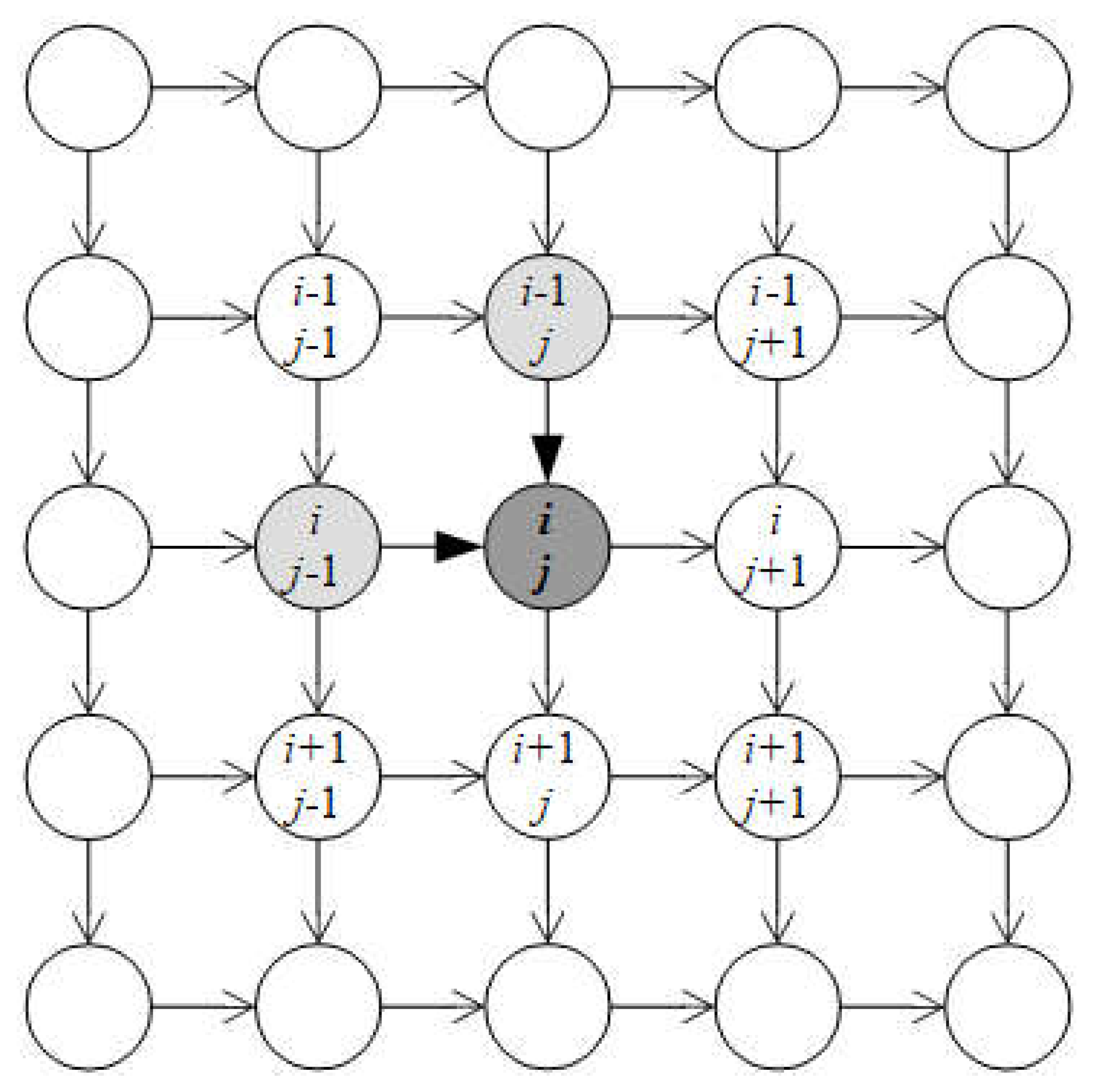
The equations above specify core ideology of PD associated with two-dimension LSTM where the contextual meaning of weight and bias parameters W_(.), U_(.), V_(.), and b_(.) is not changed with note that W_(.), U_(.), and V_(.) are weight matrices regarding current pixel, previous pixel (i, j–1), and previous pixel (i–1, j), respectively. In literature, such PD is called PixelRNN associated with diagonal two-dimension LSTM (Oord, Kalchbrenner, & Kavukcuoglu, 2016, pp. 3-4). According to diagonal two-dimension LSTM each pixel (i, j) at i^th row and j^th column has two previous neighbors such as previous left pixel (i, j–1) and previous upper pixel (i–1, j). For extension, each pixel (i, j) can have up four previous neighbors such as pixel (i, j–1), pixel (i–1, j–1), pixel (i–1, j), and pixel (i–1, j+1). Following figure depicts PixelRNN with diagonal two-dimension LSTM (Oord, Kalchbrenner, & Kavukcuoglu, 2016, p. 4).

Figure 2.1. PixelRNN with diagonal two-dimension LSTM.

Figure 2.1. PixelRNN with diagonal two-dimension LSTM.

It is easy to add more weight parameters to these extensive cases. For example, cell gates and cell state with regard to the four previous neighbors are specified as follows:

$$\begin{array}{l}{\mathit{i}}_{i,j}={\sigma }_{\mathit{i}}\left({\mathit{W}}_{\mathit{i}}{\mathit{x}}_{i,j}+{\mathit{U}}_{\mathit{i}}{\mathit{h}}_{i,j-1}+{\mathit{V}}_{\mathit{i}}{\mathit{h}}_{i-1,j}+{\mathit{R}}_{\mathit{i}}{\mathit{h}}_{i-1,j-1}+{\mathit{S}}_{\mathit{i}}{\mathit{h}}_{i-1,j+1}+{\mathit{b}}_{\mathit{i}}\right)\\ {\mathit{f}}_{i,j}={\sigma }_{\mathit{f}}\left({\mathit{W}}_{\mathit{f}}{\mathit{x}}_{i,j}+{\mathit{U}}_{\mathit{f}}{\mathit{h}}_{i,j-1}+{\mathit{V}}_{\mathit{f}}{\mathit{h}}_{i-1,j}+{\mathit{R}}_{\mathit{f}}{\mathit{h}}_{i-1,j-1}+{\mathit{S}}_{\mathit{f}}{\mathit{h}}_{i-1,j+1}+{\mathit{b}}_{\mathit{f}}\right)\\ {\mathit{o}}_{i,j}={\sigma }_{\mathit{o}}\left({\mathit{W}}_{\mathit{o}}{\mathit{x}}_{i,j}+{\mathit{U}}_{\mathit{o}}{\mathit{h}}_{i,j-1}+{\mathit{V}}_{\mathit{o}}{\mathit{h}}_{i-1,j}+{\mathit{R}}_{\mathit{o}}{\mathit{h}}_{i-1,j-1}+{\mathit{S}}_{\mathit{o}}{\mathit{h}}_{i-1,j+1}+{\mathit{b}}_{\mathit{i}}\right)\\ {\mathit{g}}_{i,j}={\sigma }_{\mathit{g}}\left({\mathit{W}}_{\mathit{g}}{\mathit{x}}_{i,j}+{\mathit{U}}_{\mathit{g}}{\mathit{h}}_{i,j-1}+{\mathit{V}}_{\mathit{g}}{\mathit{h}}_{i-1,j}+{\mathit{R}}_{\mathit{g}}{\mathit{h}}_{i-1,j-1}+{\mathit{S}}_{\mathit{g}}{\mathit{h}}_{i-1,j+1}+{\mathit{b}}_{\mathit{g}}\right)\\ {\mathit{c}}_{i,j}={\mathit{f}}_{i,j}⨂\left({\mathit{c}}_{i,j-1}+{\mathit{c}}_{i-1,j}+{\mathit{c}}_{i-1,j-1}+{\mathit{c}}_{i-1,j+1}\right)+{\mathit{i}}_{i,j}⨂{\mathit{g}}_{i,j}\\ {\mathit{h}}_{i,j}={\mathit{o}}_{i,j}⨂{\sigma }_{\mathit{h}}\left({\mathit{c}}_{i,j}\right)\end{array}$$

Where matrices R_(.) and S_(.) are additional weight parameters regarding two new neighbor pixels such as pixel (i–1, j–1) and pixel (i–1, j+1).

Recall that c_i,j is considered as evaluated value of pixel x_i,j and h_i,j is predictive value of pixel x_i,j. It is interesting that h_i,j is generated pixel within the aforementioned generation process by PD. Turning back the generation process, without loss of generality, given k randomized pixels x_i–1,1, x_i–1,2,.., x_i–1,j+1,…, x_i,1, x_i,2,…, x_i,j, we will generate the next pixel x_i,j+1. Firstly, PD model must be trained by some dataset as a set of images. Secondly, k randomized pixels x_i–1,1, x_i–1,2,.., x_i–1,j+1,…, x_i,1, x_i,2,…, x_i,j are fed to PD again so as to update k sets of parameters W_(.), U_(.), and b_(.) as well as compute k predictive values h_i–1,1, h_i–1,2,.., h_i–1,j+1,…, h_i,1, h_i,2,…, h_i,j. Finally, it is possible to determine the predictive value h_i,j+1 of the next pixel (i, j+1) given x_i,j+1, h_i,j, and h_i–1,j+1 along with learned parameters of two-dimension LSTM PD. It is important to note that x_i,j+1 is randomized arbitrarily whereas h_i,j and h_i–1,j+1 were computed previously. Obviously, it is easy to generate next predictive values h_i,j+2, h_i,j+2,…, h_i+1,j, h_i+1,j+1, etc. by the similar process. Note, backpropagation algorithm can be applied into learning two-dimension LSTM as usual. Note, backpropagation algorithm is often associated with stochastic gradient descent (SGD) method and so, please pay attention to SGD.

3. Approximate Density DGM

According to approximate density approach, DGMs try to estimate approximately generator PDF P(x | Φ, z) or derive other PDF that is similar to P(x | Φ, z) with note that PDF is abbreviation of probability density function.

Recall that there are two problems related to construct a DGM: 1) how to define likelihood or error to train generator DNN g(z | Φ) and 2) how to define tractable PDF P(z) which implies the way to randomize z. The second problem relates to assert qualification of random data z’ and hence, the second problem is stated as qualification problem of how to qualify random data. According to implicit density approach, a discrimination DNN is used to qualify randomized data z instead of defining tractable PDF P(z) by Generative Adversarial Network (GAN) which is a typical method belonging to implicit density approach. In different way belonging to this approximate density approach, Variational Autoencoders (VAE) method developed by Kingma and Welling (Kingma & Welling, 2022) proposed another DNN called encoder f(x | Θ) to expectedly convert intractable data x into tractable data z. In other words, encoder f(x | Θ) approximates tractable data z by encoded data z’.

$$f\left(\mathit{x}|\mathsf{\Theta }\right)={\mathit{z}}^{\prime }\cong \mathit{z}$$

(3.1)

It is easy to recognize that encoder f(x | Θ) is an approximation of the inverse of generator g(z | Φ) when g(z | Φ) is invertible where x-dimension m is larger than z-dimension n (m > n), which is the reason that generator g(z | Φ) is called decoder g(z | Φ) in VAE. Like decoder g(z | Φ), encoder f(x | Θ) is modeled by a so-called encoder DNN whose weights are parameter Θ called encoder parameter and so parameter Φ is called decoder parameter in VAE. By following the fact that encoder f(x | Θ) approximates tractable data z by encoded data z’, tractable PDF P(z) is approximated by a so-called encoder PDF P_f(z’).

$$P_f\left({\mathit{z}}^{\prime }\right)\cong P\left(\mathit{z}\right)$$

Because encoder f(x | Θ) depends on its parameter Θ, we can denote:

$$P_f\left({\mathit{z}}^{\prime }\right)=P\left({\mathit{z}}^{\prime }|\mathsf{\Theta },\mathit{x}\right)$$

Essential, encoder PDF P(z’ | Θ, x) is likelihood function of z’ given x which is conditional PDF of z’ given x and hence, P(z’ | Θ, x) is called encoder likelihood which depends on encoder f(x | Θ), of course. On the other hand, P(z’ | Θ, x) is posterior PDF of tractable data given tractable data x where P(z) is prior PDF of tractable data. In practice, z’ is assumed to conform multivariate normal distribution and therefore, let μ(x) and Σ(x) be mean vector and covariance matrix of z’. Encoder likelihood P(z’ | Θ, x) becomes P(z’ | Θ, μ(x | Θ), Σ(x | Θ)) so that output of encoder DNN f(x | Θ) is mean μ(x | Θ) and covariance matrix Σ(x | Θ) while its input is x and its weights are Θ, of course.

$$\begin{array}{l}f\left(\mathit{x}|\mathsf{\Theta }\right)=\left(\begin{array}{c}\mu \left(\mathit{x}|\mathsf{\Theta }\right)\\ \mu \left(\mathit{x}|\mathsf{\Theta }\right)\end{array}\right)\\ P\left({\mathit{z}}^{\prime }|\mathsf{\Theta },\mathit{x}\right)=P\left({\mathit{z}}^{\prime }|\mathsf{\Theta },\mu \left(\mathit{x}\right),\mathsf{\Sigma }\left(\mathit{x}\right)\right)=\mathcal{N}\left(\mathit{z}|\mu \left(\mathit{x}|\mathsf{\Theta }\right),\mathsf{\Sigma }\left(\mathit{x}|\mathsf{\Theta }\right)\right)\end{array}$$

(3.2)

Note, $\mathcal{N}$(.) denotes normal distribution and thus, $\mathcal{N}$(z | μ(x | Θ), Σ(x | Θ)) represents encoder likelihood. That $\mathcal{N}$(z | μ(x | Θ), Σ(x | Θ)) is encoder likelihood is an important improvement in developing VAE because encoder DNN f(x | Θ) is learned by minimizing a so-called encoder error which is represented by the difference between encoder likelihood and predefined tractable PDF P(z). Let KL($\mathcal{N}$(z | μ(x | Θ), Σ(x | Θ)) | P(z)) be Kullback-Leibler divergence of encoder likelihood $\mathcal{N}$(z | μ(x | Θ), Σ(x | Θ)) and predefined tractable PDF P(z). As a result, KL($\mathcal{N}$(z | μ(x | Θ), Σ(x | Θ)) | P(z)) becomes an ideal encoder error, which is called encoder KL divergence. The smaller the encoder KL divergence is, the closer the encoder likelihood $\mathcal{N}$(z | μ(x | Θ), Σ(x | Θ)) is to tractable PDF P(z), the better the encoder DNN f(x | Θ) is.

$$\epsilon \left(\mu \left(\mathit{x}|\mathsf{\Theta }\right),\mathsf{\Sigma }\left(\mathit{x}|\mathsf{\Theta }\right)|\mathsf{\Theta }\right)=\mathrm{K}\mathrm{L}\left(\mathcal{N}\left(\mathit{z}|\mu \left(\mathit{x}|\mathsf{\Theta }\right),\mathsf{\Sigma }\left(\mathit{x}|\mathsf{\Theta }\right)\right)|P\left(\mathit{z}\right)\right)$$

(3.3)

Therefore, encoder KL divergence KL($\mathcal{N}$(z | μ(x | Θ), Σ(x | Θ)) | P(z)) is minimized by stochastic gradient descent (SGD) method in order to estimate decoder parameter Θ for training encoder DNN f(x | Θ) as follows:

$${\mathsf{\Theta }}^{*}=\underset{\mathsf{\Theta }}{\mathrm{armin}}\mathrm{K}\mathrm{L}\left(\mathcal{N}\left(\mathit{z}|\mu \left(\mathit{x}|\mathsf{\Theta }\right),\mathsf{\Sigma }\left(\mathit{x}|\mathsf{\Theta }\right)\right)|P\left(\mathit{z}\right)\right)$$

Which results estimation equation according to SGD:

$$\mathsf{\Theta }=\mathsf{\Theta }-\gamma \nabla \mathrm{K}\mathrm{L}\left(\mathcal{N}\left(\mathit{z}|\mu \left(\mathit{x}|\mathsf{\Theta }\right),\mathsf{\Sigma }\left(\mathit{x}|\mathsf{\Theta }\right)\right)|P\left(\mathit{z}\right)\right)$$

Where ∇KL($\mathcal{N}$(z | μ(x | Θ), Σ(x | Θ)) | P(z)) is gradient of encoder KL divergence KL($\mathcal{N}$(z | μ(x | Θ), Σ(x | Θ)) | P(z)) with regard to μ(x | Θ) and Σ(x | Θ) while γ is learning rate. Recall that SGD, which is an iterative process, pushes candidate solution at each iteration along the direction which is opposite to gradient of target function for minimization or has the same direction to gradient of target function for maximization with note that the step length is represented by learning rate. We have:

$$\nabla \mathrm{K}\mathrm{L}\left(\mathcal{N}\left(\mathit{z}|\mu \left(\mathit{x}|\mathsf{\Theta }\right),\mathsf{\Sigma }\left(\mathit{x}|\mathsf{\Theta }\right)\right)|P\left(\mathit{z}\right)\right)=\frac{d\mathrm{K}\mathrm{L}\left(\mathcal{N}\left(\mathit{z}|\mu \left(\mathit{x}|\mathsf{\Theta }\right),\mathsf{\Sigma }\left(\mathit{x}|\mathsf{\Theta }\right)\right)|P\left(\mathit{z}\right)\right)}{d\mathsf{\Theta }}$$

There can be no change in estimating decoder parameter Φ within VAE so that decoder error ε(x | Φ, z) = ½||g(z | Φ) – x||² is minimized to produce optimal Φ.

$${\mathsf{\Phi }}^{*}=\underset{\mathsf{\Phi }}{\mathrm{armin}}\frac{1}{2}{‖g\left(\mathit{z}|\mathsf{\Phi }\right)-\mathit{x}‖}^2$$

Which results estimation equation according to SGD:

$$\mathsf{\Phi }=\mathsf{\Phi }-\gamma \nabla \frac{1}{2}{‖g\left(\mathit{z}|\mathsf{\Phi }\right)-\mathit{x}‖}^2$$

Recall that generator g(z | Φ) is called decoder g(z | Φ) in VAE. As a result, encoder parameter Θ and decoder parameter Φ are estimated as follows:

$$\begin{array}{l}\mathsf{\Theta }=\mathsf{\Theta }-\gamma \nabla \mathrm{K}\mathrm{L}\left(\mathcal{N}\left(\mathit{z}|\mu \left(\mathit{x}|\mathsf{\Theta }\right),\mathsf{\Sigma }\left(\mathit{x}|\mathsf{\Theta }\right)\right)|P\left(\mathit{z}\right)\right)\\ \mathsf{\Phi }=\mathsf{\Phi }-\gamma \nabla \frac{1}{2}{‖g\left(\mathit{z}|\mathsf{\Phi }\right)-\mathit{x}‖}^2=\mathsf{\Phi }-\gamma \left(g\left(\mathit{z}|\mathsf{\Phi }\right)-\mathit{x}\right)\frac{dg\left(\mathit{z}|\mathsf{\Phi }\right)}{d\mathsf{\Phi }}\end{array}$$

Where dg(z | Φ) / dΦ is differential of g(z | Φ) with regard to Φ while 0 < γ ≤ 1 is learning rate and tractable PDF P(z) is predefined with note that VAE replaces tractable PDF P(z) by likelihood P(z’ | Θ, μ(x | Θ), Σ(x | Θ)) with fixed P(z). As usual, P(z) is assumed to conform standard normal distribution with mean 0 and covariance matrix I.

$$P\left(\mathit{z}\right)=\mathcal{N}\left(\mathit{z}|0,I\right)$$

This implies:

$$\mathsf{\Theta }=\mathsf{\Theta }-\gamma \nabla \mathrm{K}\mathrm{L}\left(\mathcal{N}\left(\mathit{z}|\mu \left(\mathit{x}|\mathsf{\Theta }\right),\mathsf{\Sigma }\left(\mathit{x}|\mathsf{\Theta }\right)\right)|\mathcal{N}\left(\mathit{z}|0,I\right)\right)$$

Where I is identity matrix:

$$I=\left(\begin{array}{cccc}1& 0& \cdots & 0\\ 0& 1& \cdots & 0\\ ⋮& ⋮& \ddots & ⋮\\ 0& 0& \cdots & 1\end{array}\right)$$

It is easier to determine gradient of encoder KL divergence ∇KL(N(μ(x | Θ), Σ(x | Θ)) | $\mathcal{N}$(z | 0, I)) with regard to Θ between the multivariate normal distribution $\mathcal{N}$(μ(x), Σ(x) | Θ) and the standard multivariate normal distribution $\mathcal{N}$(z | 0, I)). We have following equation to calculate such gradient (Kingma & Welling, 2022, p. 5), (Doersch, 2016, p. 9), (Nguyen, 2015, p. 43):

$$\begin{array}{l}\nabla \mathrm{K}\mathrm{L}\left(\mathcal{N}\left(\mathit{z}|\mu \left(\mathit{x}|\mathsf{\Theta }\right),\mathsf{\Sigma }\left(\mathit{x}|\mathsf{\Theta }\right)\right)|\mathcal{N}\left(\mathit{z}|0,I\right)\right)=\frac{d\mathrm{K}\mathrm{L}\left(\mathcal{N}\left(\mathit{z}|\mu \left(\mathit{x}|\mathsf{\Theta }\right),\mathsf{\Sigma }\left(\mathit{x}|\mathsf{\Theta }\right)\right)|\mathcal{N}\left(\mathit{z}|0,I\right)\right)}{d\mathsf{\Theta }}\\ ={\left(\begin{array}{l}\mu \left(\mathit{x}|\mathsf{\Theta }\right)\frac{d\mu \left(\mathit{x}|\mathsf{\Theta }\right)}{d\mathsf{\Theta }}\\ \frac{1}{2}\left(I-{\left(\mathsf{\Sigma }\left(\mathit{x}|\mathsf{\Theta }\right)\right)}^{-1}\right)\frac{d\mathsf{\Sigma }\left(\mathit{x}|\mathsf{\Theta }\right)}{d\mathsf{\Theta }}\end{array}\right)}^T\\ =\left(\mu \left(\mathit{x}|\mathsf{\Theta }\right)\frac{d\mu \left(\mathit{x}|\mathsf{\Theta }\right)}{d\mathsf{\Theta }},\frac{1}{2}\left(I-{\left(\mathsf{\Sigma }\left(\mathit{x}|\mathsf{\Theta }\right)\right)}^{-1}\right)\frac{d\mathsf{\Sigma }\left(\mathit{x}|\mathsf{\Theta }\right)}{d\mathsf{\Theta }}\right)\end{array}$$

Where (Σ(x | Θ))^–1 is inverse of covariance matrix Σ(x | Θ) and the subscript “T” denotes transposition operator of matrix and vector whereas dμ(x | Θ) / dΘ and dΣ(x | Θ) / dΘ are differentials of μ(x | Θ) and Σ(x | Θ) with regard to Θ, respectively. As a result, encoder parameter Θ and decoder parameter Φ are totally estimated according to SGD as follows:

$$\begin{array}{l}\mathsf{\Theta }=\mathsf{\Theta }-\gamma \left(\begin{array}{l}\mu \left(\mathit{x}|\mathsf{\Theta }\right)\frac{d\mu \left(\mathit{x}|\mathsf{\Theta }\right)}{d\mathsf{\Theta }}\\ \frac{1}{2}\left(I-{\left(\mathsf{\Sigma }\left(\mathit{x}|\mathsf{\Theta }\right)\right)}^{-1}\right)\frac{d\mathsf{\Sigma }\left(\mathit{x}|\mathsf{\Theta }\right)}{d\mathsf{\Theta }}\end{array}\right)\\ \mathsf{\Phi }=\mathsf{\Phi }-\gamma \left(g\left(\mathit{z}|\mathsf{\Phi }\right)-\mathit{x}\right)\frac{dg\left(\mathit{z}|\mathsf{\Phi }\right)}{d\mathsf{\Phi }}\end{array}$$

The estimation equations above are simple explanation of VAE but its formal construction is more complicated. We begin the aforementioned intractable PDF P(x) specified by law of total probability:

$$P\left(\mathit{x}\right)=\underset{\mathit{z}}{\int }P\left(\mathit{x}|\mathsf{\Phi },\mathit{z}\right)P\left(\mathit{z}\right)d\mathit{z}$$

However, P(x) is interpreted by another way which is based on Bayes’ rule within VAE:

$$P\left(\mathit{x}\right)=\frac{P\left(\mathit{x},\mathit{z}\right)}{P\left(\mathit{z}|\mathit{x}\right)}$$

Because the conditional probability P(z | x) is arbitrary without formal specification, it should be approximated by another PDF denoted Q(z | x) with assumption that the PDF Q(z | x) has formal specification like normal distribution.

$$Q\left(\mathit{z}|\mathit{x}\right)\cong P\left(\mathit{z}|\mathit{x}\right)$$

Logarithm of intractable PDF P(x) is specified as follows (Ruthotto & Haber, 2021, p. 13):

$$\log P\left(\mathit{x}\right)=\log \frac{P\left(\mathit{x},\mathit{z}\right)}{P\left(\mathit{z}|\mathit{x}\right)}=\log \left(\frac{P\left(\mathit{x},\mathit{z}\right)}{Q\left(\mathit{z}|\mathit{x}\right)}\frac{Q\left(\mathit{z}|\mathit{x}\right)}{P\left(\mathit{z}|\mathit{x}\right)}\right)$$

This implies:

$$\log P\left(\mathit{x}\right)=\log \frac{P\left(\mathit{x},\mathit{z}\right)}{Q\left(\mathit{z}|\mathit{x}\right)}+\log \frac{Q\left(\mathit{z}|\mathit{x}\right)}{P\left(\mathit{z}|\mathit{x}\right)}$$

(3.4)

The second term log(Q(z | x) / P(z | x)) is not variant because Q(z | x) is approximated to P(z | x). Therefore, the first term log(P(x, z) / Q(z | x) is called variation lower bound or evidence lower bound because it is variant. Let l(x, z) be loss function or error function on VAE which is defined as the minus opposite of expectation of the evidence lower bound log(P(x, z) / Q(z | x) given PDF Q(z | x) with note that Q(z | x) has formal probabilistic distribution.

$$l\left(\mathit{x},\mathit{z}\right)=-E_{Q\left(\mathit{z}|\mathit{x}\right)}\left(\log \frac{P\left(\mathit{x},\mathit{z}\right)}{Q\left(\mathit{z}|\mathit{x}\right)}\right)=-\underset{\mathit{z}}{\int }Q\left(\mathit{z}|\mathit{x}\right)\log \frac{P\left(\mathit{x}|\mathit{z}\right)P\left(\mathit{z}\right)}{Q\left(\mathit{z}|\mathit{x}\right)}d\mathit{z}$$

Loss function l(x, z) is expended as follows:

$$\begin{gathered} l\left(\mathit{x},\mathit{z}\right)=-\log P\left(\mathit{x}|\mathit{z}\right)\underset{\mathit{z}}{\int }Q\left(\mathit{z}|\mathit{x}\right)d\mathit{z}+\underset{\mathit{z}}{\int }Q\left(\mathit{z}|\mathit{x}\right)\left(\log \frac{Q\left(\mathit{z}|\mathit{x}\right)}{P\left(\mathit{z}\right)}\right)d\mathit{z} \\ =-\log P\left(\mathit{x}|\mathit{z}\right)+\underset{\mathit{z}}{\int }Q\left(\mathit{z}|\mathit{x}\right)\left(\log \frac{Q\left(\mathit{z}|\mathit{x}\right)}{P\left(\mathit{z}\right)}\right)d\mathit{z} \end{gathered}$$

Because Q(z | x) and P(x | z) depend on encoder f(x | Θ) and decoder g(z | Φ), respectively, their parameters are Θ and Φ, respectively.

$$\begin{gathered} Q\left(\mathit{z}|\mathit{x}\right)=Q\left(\mathit{z}|\mathsf{\Theta },\mathit{x}\right) \\ P\left(\mathit{x}|\mathit{z}\right)=P\left(\mathit{x}|\mathsf{\Phi },\mathit{z}\right) \end{gathered}$$

Exactly, Q(z | Θ, x) is encoder likelihood which is the same to the aforementioned P(z’ | Θ, x) except that it is focused that Q(z | Θ, x) has formal probabilistic specification like normal distribution. Loss function l(Θ, Φ | x, z), which is now function of encoder parameter Θ and decoder parameter Φ, is written as follows (Ruthotto & Haber, 2021, p. 14):

$$l\left(\mathsf{\Theta },\mathsf{\Phi }|\mathit{x},\mathit{z}\right)=-\log P\left(\mathit{x}|\mathsf{\Phi },\mathit{z}\right)+\underset{\mathit{z}}{\int }Q\left(\mathit{z}|\mathsf{\Theta },\mathit{x}\right)\left(\log \frac{Q\left(\mathit{z}|\mathsf{\Theta },\mathit{x}\right)}{P\left(\mathit{z}\right)}\right)d\mathit{z}$$

Firstly, please pay attention to the first term loss function l(Θ, Φ | x, z) where P(x | Φ, z) depends only on Φ although it can be considered as a conditional PDF of x given z because P(x | Φ, z) is defined for output layer containing only x of decoder DNN g(x | Φ) whose input is x. Therefore, we had the following assertion:

$$\underset{\mathit{z}}{\int }Q\left(\mathit{z}|\mathit{x}\right)\log P\left(\mathit{x}|\mathsf{\Phi },\mathit{z}\right)d\mathit{z}=\log P\left(\mathit{x}|\mathsf{\Phi },\mathit{z}\right)\underset{\mathit{z}}{\int }Q\left(\mathit{z}|\mathit{x}\right)d\mathit{z}=\log P\left(\mathit{x}|\mathsf{\Phi },\mathit{z}\right)=\log P\left(\mathit{x}|\mathsf{\Phi }\right)$$

Secondly, the second term in loss function l(Θ, Φ | x, z) is, actually, Kullback-Leibler divergence of encoder likelihood Q(z | Θ, x) and predefined tractable PDF P(z), which measure the difference between Q(z | Θ, x) and P(z). As a convention, this Kullback-Leibler divergence is called encoder KL divergence which is an ideal encoder error.

$$\mathrm{K}\mathrm{L}\left(Q\left(\mathit{z}|\mathsf{\Theta },\mathit{x}\right)|P\left(\mathit{z}\right)\right)=E_{Q\left(\mathit{z}|\mathit{x}\right)}\left(\log \frac{Q\left(\mathit{z}|\mathsf{\Theta },\mathit{x}\right)}{P\left(\mathit{z}\right)}\right)=\underset{\mathit{z}}{\int }Q\left(\mathit{z}|\mathsf{\Theta },\mathit{x}\right)\left(\log \frac{Q\left(\mathit{z}|\mathsf{\Theta },\mathit{x}\right)}{P\left(\mathit{z}\right)}\right)d\mathit{z}$$

The smaller the encoder KL divergence is, the closer the encoder likelihood Q(z | Θ, x) is to tractable PDF P(z), the better the encoder DNN f(x | Θ) is. Loss function is rewritten again:

$$l\left(\mathsf{\Theta },\mathsf{\Phi }|\mathit{x},\mathit{z}\right)=-\log P\left(\mathit{x}|\mathsf{\Phi },\mathit{z}\right)+\mathrm{K}\mathrm{L}\left(Q\left(\mathit{z}|\mathsf{\Theta },\mathit{x}\right)|P\left(\mathit{z}\right)\right)$$

Or,

$$l\left(\mathsf{\Theta },\mathsf{\Phi }|\mathit{x},\mathit{z}\right)=-\log P\left(\mathit{x}|\mathsf{\Phi }\right)+\mathrm{K}\mathrm{L}\left(Q\left(\mathit{z}|\mathsf{\Theta }\right)|P\left(\mathit{z}\right)\right)$$

(3.5)

According to the two problem of construct a DGM, the first term –log(P(x | Φ, z)) in loss function indicates the first problem of how to train decoder DNN g(z | Φ) which is called reconstruction error in literature and the second term KL(Q(z | Θ, x) | P(z)) in loss function indicates the second problem of how to qualify training task for training encoder DNN f(x | Θ) which is called regularity in literature. Loss function l(Θ, Φ | x, z) is minimized to estimate Θ and Φ as follows:

$$\begin{array}{l}{\mathsf{\Theta }}^{*}=\underset{\mathsf{\Theta }}{\mathrm{armin}}l\left(\mathsf{\Theta },\mathsf{\Phi }|\mathit{x},\mathit{z}\right)\\ {\mathsf{\Phi }}^{*}=\underset{\mathsf{\Phi }}{\mathrm{armin}}l\left(\mathsf{\Theta },\mathsf{\Phi }|\mathit{x},\mathit{z}\right)\end{array}$$

(3.6)

Because P(x | Θ, z) depends only on Θ and encoder KL divergence KL(Q(z | Θ, x) | P(z)) depends only on Φ, the optimization problem is specified as follows:

$$\begin{array}{l}{\mathsf{\Theta }}^{*}=\underset{\mathsf{\Theta }}{\mathrm{armin}}\mathrm{K}\mathrm{L}\left(Q\left(\mathit{z}|\mathsf{\Theta },\mathit{x}\right)|P\left(\mathit{z}\right)\right)\\ {\mathsf{\Phi }}^{*}=\underset{\mathsf{\Phi }}{\mathrm{armin}}\left(-\log P\left(\mathit{x}|\mathsf{\Phi },\mathit{z}\right)\right)=\underset{\mathsf{\Phi }}{\mathrm{armax}}\left(\log P\left(\mathit{x}|\mathsf{\Phi },\mathit{z}\right)\right)\end{array}$$

Which results estimation equations according to SGD:

$$\begin{array}{l}\mathsf{\Theta }=\mathsf{\Theta }-\gamma \nabla \mathrm{K}\mathrm{L}\left(Q\left(\mathit{z}|\mathsf{\Theta },\mathit{x}\right)|P\left(\mathit{z}\right)\right)\\ \mathsf{\Phi }=\mathsf{\Phi }+\gamma \nabla \log P\left(\mathit{x}|\mathsf{\Phi },\mathit{z}\right)\end{array}$$

(3.7)

Where ∇KL(Q(z | Θ, x) | P(z)) is gradient of encoder KL divergence KL(Q(z | Θ, x) | P(z)) with regard to encoder parameter Θ. Note that tractable PDF P(z) is predefined (fixed). While Q(z | Θ, x) is called encoder likelihood, P(x | Φ, z) is called decoder likelihood. On the other hand, while P(z) is prior PDF of intractable data z, then Q(z | Θ, x) is approximated posterior PDF of z given x where both P(z) and Q(z | Θ, x) have formal probabilistic specifications and moreover, P(z) is fixed (predefined).

$$Q\left(\mathit{z}|\mathsf{\Theta },\mathit{x}\right)=P\left({\mathit{z}}^{\prime }|\mathsf{\Theta },\mathit{x}\right)\cong P\left(\mathit{z}|\mathsf{\Theta },\mathit{x}\right)$$

Both P(z | Θ, x) and Q(z | Θ, x) are encoder likelihood as well as posterior PDF of tractable data z but Q(z | Θ, x) is approximated one whose probabilistic distribution is specified formally. Therefore (Ruthotto & Haber, 2021, p. 16), randomized data z’ in latent space Z is sampled from approximated distribution Q(z | Θ, x) instead of sampling from true distribution P(z | Θ, x).

Given epoch of size N is denoted as D = (d⁽¹⁾ = (x⁽¹⁾, z⁽¹⁾), d⁽²⁾ = (x⁽²⁾, z⁽²⁾),…, d^(N) = (x^(N), z^(N))), the estimation equations of Θ and Φ are extended exactly as epoch estimation at every iteration of SGD:

$$\begin{array}{l}{\mathsf{\Theta }}^{\left(k+1\right)}={\mathsf{\Theta }}^{\left(k\right)}-\gamma \nabla \frac{1}{N}{\displaystyle \sum _{i=1}^N}\mathrm{K}\mathrm{L}\left(Q\left({\mathit{z}}^{\left(i\right)}|{\mathsf{\Theta }}^{\left(k\right)},{\mathit{x}}^{\left(i\right)}\right)|P\left(\mathit{z}\right)\right)\\ {\mathsf{\Phi }}^{\left(k+1\right)}={\mathsf{\Phi }}^{\left(k\right)}+\gamma \nabla \frac{1}{N}{\displaystyle {\displaystyle \sum _{i=1}^N}}\log P\left({\mathit{x}}^{\left(i\right)}|\mathsf{\Phi },{\mathit{z}}^{\left(i\right)}\right)\end{array}$$

Please distinguish that the tractable data z⁽ⁱ⁾ in the first equation above follows distribution P(z) but the tractable data z⁽ⁱ⁾ in the second equation above follows distribution Q(z | Θ, x). As a result, VAE trained with SGD is specified as follows:

Initialize Θ and Φ and set k = 0.

Repeat

Sampling epoch X = (x⁽¹⁾, x⁽²⁾,…, x^(N)) or receiving epoch X from big data / data stream.

Randomize random epoch Z = (z⁽¹⁾, z⁽²⁾,…, z^(N)) in which each z⁽ⁱ⁾ is randomized from distribution Q(z | Θ^(k), x⁽ⁱ⁾).

$$\begin{array}{l}{\mathsf{\Theta }}^{\left(k+1\right)}={\mathsf{\Theta }}^{\left(k\right)}-\gamma \nabla \frac{1}{N}{\displaystyle \sum _{i=1}^N}\mathrm{K}\mathrm{L}\left(Q\left({\mathit{z}}^{\left(i\right)}|{\mathsf{\Theta }}^{\left(k\right)},{\mathit{x}}^{\left(i\right)}\right)|P\left(\mathit{z}\right)\right)\\ {\mathsf{\Phi }}^{\left(k+1\right)}={\mathsf{\Phi }}^{\left(k\right)}+\gamma \nabla \frac{1}{N}{\displaystyle \sum _{i=1}^N}\log P\left({\mathit{x}}^{\left(i\right)}|\mathsf{\Phi },{\mathit{z}}^{\left(i\right)}\right)\end{array}$$

Increase k = k + 1.

Until some terminating conditions are met.

Note, a terminating condition is customized, for example, parameters Θ and Φ are not changed significantly or there is no more coming epoch X. Moreover, the index k indicates time point as well as iteration of SGD. Because PDF P(z) is predefined, it is easy to calculate encoder KL divergence KL(Q(z⁽ⁱ⁾ | Θ^(k), x⁽ⁱ⁾) | P(z)) but it is necessary to define P(x) by well-known distribution. However, randomizing random epoch Z = (z⁽¹⁾, z⁽²⁾,…, z^(N)) from distribution Q(z | Θ^(k), x⁽ⁱ⁾)) is not easy and so, VAE trained with SGD will be fine-tuned. It is interesting that when Q(z | Θ^(k), x⁽ⁱ⁾)) is posterior PDF of z and P(z) is prior PDF of z, the event that z is randomized from the posterior PDF Q(z | Θ^(k), x⁽ⁱ⁾)) and Q(z | Θ^(k), x⁽ⁱ⁾)) itself is updated continuously based on its previous evidence x⁽ⁱ⁾ over SGD iterations implies that VAE conforms Bayesian statistics in estimation. Moreover, P(z) is an alignment that Q(z | Θ^(k), x⁽ⁱ⁾)) adjusts itself with support of encoder KL divergence KL(Q(z⁽ⁱ⁾ | Θ^(k), x⁽ⁱ⁾) | P(z)).

Because encoder likelihood Q(z | Θ, x) must always have formal probabilistic distribution, it is assumed to follow multivariate normal distribution in practice. Therefore, let μ(x | Θ) and Σ(x | Θ) be mean vector and covariance matrix of z, then encoder likelihood Q(z | Θ, x) becomes Q(z | μ(x | Θ), Σ(x | Θ)) so that output of encoder DNN f(x | Θ) is mean μ(x | Θ) and covariance matrix Σ(x | Θ) while its input is x and its weights are Θ, of course. Please pay attention to the fact that output of encoder DNN f(x | Θ) is now μ(x | Θ) and Σ(x | Θ) which are corresponding to z. Moreover, μ(x | Θ) and Σ(x | Θ) are functions of x, whose parameter is Θ.

$$\begin{array}{l}f\left(\mathit{x}|\mathsf{\Theta }\right)=\left(\begin{array}{c}\mu \left(\mathit{x}|\mathsf{\Theta }\right)\\ \mathsf{\Sigma }\left(\mathit{x}|\mathsf{\Theta }\right)\end{array}\right)~\mathit{z}\\ Q\left(\mathit{z}|\mu \left(\mathit{x}|\mathsf{\Theta }\right),\mathsf{\Sigma }\left(\mathit{x}|\mathsf{\Theta }\right)\right)=\mathcal{N}\left(\mathit{z}|\mu \left(\mathit{x}|\mathsf{\Theta }\right),\mathsf{\Sigma }\left(\mathit{x}|\mathsf{\Theta }\right)\right)\end{array}$$

(3.8)

Note, $\mathcal{N}$(z | μ(x | Θ), Σ(x | Θ)) denotes multivariate normal distribution with mean μ(x | Θ) and covariance matrix Σ(x | Θ).

$$\begin{array}{l}\mathcal{N}\left(\mathit{z}|\mu \left(\mathit{x}|\mathsf{\Theta }\right),\mathsf{\Sigma }\left(\mathit{x}|\mathsf{\Theta }\right)\right)\\ ={\left(2\pi \right)}^{-\frac{n}{2}}{\left|\mathsf{\Sigma }\left(\mathit{x}|\mathsf{\Theta }\right)\right|}^{-\frac{1}{2}}\mathrm{e}\mathrm{x}\mathrm{p}\left(-\frac{1}{2}{\left(\mathit{z}-\mu \left(\mathit{x}|\mathsf{\Theta }\right)\right)}^T{\left(\mathsf{\Sigma }\left(\mathit{x}|\mathsf{\Theta }\right)\right)}^{-1}(\mathit{z}-\mu \left(\mathit{x}|\mathsf{\Theta }\right))\right)\end{array}$$

Note, dimension of tractable data z is n. Moreover, notation |.| or notation det(.) denotes determinant of matrix whereas (Σ(x | Θ))^–1 is inverse of covariance matrix Σ(x | Θ) and the subscript “T” denotes transposition operator of matrix and vector. It is easy to recognize that z’ is approximation of z. When tractable PDF P(z) is fixed, it is often assumed to follow multivariate normal distribution with predefined mean μ₀ and predefined covariance matrix Σ₀ as follows:

$$P\left(\mathit{z}\right)=\mathcal{N}\left(\mathit{z}|{\mu }_0,{\mathsf{\Sigma }}_0\right)=\mathcal{N}\left({\mu }_0,{\mathsf{\Sigma }}_0\right)={\left(2\pi \right)}^{-\frac{n}{2}}{\left|{\mathsf{\Sigma }}_0\right|}^{-\frac{1}{2}}\mathrm{e}\mathrm{x}\mathrm{p}\left(-\frac{1}{2}{\left(\mathit{z}-{\mu }_0\right)}^T{\mathsf{\Sigma }}_0^{-1}(\mathit{z}-{\mu }_0)\right)$$

Encoder KL divergence KL(Q(z | Θ, x) | P(z)) between Q(z | Θ, x) and P(z) becomes encoder KL divergence KL(Q(z | μ(x | Θ), Σ(x | Θ)) | P(z)) between Q(z | μ(x | Θ), Σ(x | Θ)) and P(z) as follows:

$$\mathrm{K}\mathrm{L}\left(Q\left(\mathit{z}|\mu \left(\mathit{x}|\mathsf{\Theta }\right),\mathsf{\Sigma }\left(\mathit{x}|\mathsf{\Theta }\right)\right)|P\left(\mathit{z}\right)\right)=\mathrm{K}\mathrm{L}\left(\mathcal{N}\left(\mathit{z}|\mu \left(\mathit{x}|\mathsf{\Theta }\right),\mathsf{\Sigma }\left(\mathit{x}|\mathsf{\Theta }\right)\right)|\mathcal{N}\left(\mathit{z}|{\mu }_0,{\mathsf{\Sigma }}_0\right)\right)$$

Which is, essentially, encoder KL divergence between two normal distributions, KL($\mathcal{N}$(z | μ(x | Θ), Σ(x | Θ)) | $\mathcal{N}$(μ₀, Σ₀)). As a convention, this divergence is called encoder KL divergence which is determined in literature as follows (Doersch, 2016, p. 9):

$$\begin{array}{l}\mathrm{K}\mathrm{L}\left(\mathcal{N}\left(\mathit{z}|\mu \left(\mathit{x}|\mathsf{\Theta }\right),\mathsf{\Sigma }\left(\mathit{x}|\mathsf{\Theta }\right)\right)|\mathcal{N}\left(\mathit{z}|{\mu }_0,{\mathsf{\Sigma }}_0\right)\right)\\ =\frac{1}{2}\left(\mathrm{t}\mathrm{r}\left({\mathsf{\Sigma }}_0^{-1}\mathsf{\Sigma }\left(\mathit{x}|\mathsf{\Theta }\right)\right)+{\left(\mu \left(\mathit{x}|\mathsf{\Theta }\right)-{\mu }_0\right)}^T{\mathsf{\Sigma }}_0^{-1}\left(\mu \left(\mathit{x}|\mathsf{\Theta }\right)-{\mu }_0\right)+\log \left(\frac{\left|{\mathsf{\Sigma }}_0\right|}{\left|\mathsf{\Sigma }\left(\mathit{x}|\mathsf{\Theta }\right)\right|}\right)-n\right)\end{array}$$

Where tr(.) denotes trace operator of square matrix which is sum of elements on main diagonal, for instance, given n_xn matrix A, then tr(A) = a₁₁ + a₂₂ +… + a_nn with note that a_ij is the element at row i and column j. Moreover, notation |.| or notation det(.) denotes determinant of matrix. Gradient of encoder KL divergence consists of two elemental gradients with regard to mean μ(x | Θ) and covariance matrix Σ(x | Θ).

$$\begin{array}{l}\nabla \mathrm{K}\mathrm{L}\left(\mathcal{N}\left(\mathit{z}|\mu \left(\mathit{x}|\mathsf{\Theta }\right),\mathsf{\Sigma }\left(\mathit{x}|\mathsf{\Theta }\right)\right)|\mathcal{N}\left(\mathit{z}|{\mu }_0,{\mathsf{\Sigma }}_0\right)\right)\\ ={\left(\begin{array}{c}{\nabla }_{\mu }\mathrm{K}\mathrm{L}\left(\mathcal{N}\left(\mathit{z}|\mu \left(\mathit{x}|\mathsf{\Theta }\right),\mathsf{\Sigma }\left(\mathit{x}|\mathsf{\Theta }\right)\right)|\mathcal{N}\left(\mathit{z}|{\mu }_0,{\mathsf{\Sigma }}_0\right)\right)\\ {\nabla }_{\mathsf{\Sigma }}\mathrm{K}\mathrm{L}\left(\mathcal{N}\left(\mathit{z}|\mu \left(\mathit{x}|\mathsf{\Theta }\right),\mathsf{\Sigma }\left(\mathit{x}|\mathsf{\Theta }\right)\right)|\mathcal{N}\left(\mathit{z}|{\mu }_0,{\mathsf{\Sigma }}_0\right)\right)\end{array}\right)}^T\end{array}$$

Where,

$$\begin{array}{l}{\nabla }_{\mu }\mathrm{K}\mathrm{L}\left(\mathcal{N}\left(\mathit{z}|\mu \left(\mathit{x}|\mathsf{\Theta }\right),\mathsf{\Sigma }\left(\mathit{x}|\mathsf{\Theta }\right)\right)|\mathcal{N}\left(\mathit{z}|{\mu }_0,{\mathsf{\Sigma }}_0\right)\right)\\ =\frac{d\mathrm{K}\mathrm{L}\left(\mathcal{N}\left(\mathit{z}|\mu \left(\mathit{x}|\mathsf{\Theta }\right),\mathsf{\Sigma }\left(\mathit{x}|\mathsf{\Theta }\right)\right)|\mathcal{N}\left(\mathit{z}|{\mu }_0,{\mathsf{\Sigma }}_0\right)\right)}{d\mu \left(\mathit{x}|\mathsf{\Theta }\right)}\frac{d\mu \left(\mathit{x}|\mathsf{\Theta }\right)}{d\mathsf{\Theta }}\\ {\nabla }_{\mathsf{\Sigma }}\mathrm{K}\mathrm{L}\left(\mathcal{N}\left(\mathit{z}|\mu \left(\mathit{x}|\mathsf{\Theta }\right),\mathsf{\Sigma }\left(\mathit{x}|\mathsf{\Theta }\right)\right)|\mathcal{N}\left(\mathit{z}|{\mu }_0,{\mathsf{\Sigma }}_0\right)\right)\\ =\frac{d\mathrm{K}\mathrm{L}\left(\mathcal{N}\left(\mathit{z}|\mu \left(\mathit{x}|\mathsf{\Theta }\right),\mathsf{\Sigma }\left(\mathit{x}|\mathsf{\Theta }\right)\right)|\mathcal{N}\left(\mathit{z}|{\mu }_0,{\mathsf{\Sigma }}_0\right)\right)}{d\mathsf{\Sigma }\left(\mathit{x}|\mathsf{\Theta }\right)}\frac{d\mathsf{\Sigma }\left(\mathit{x}|\mathsf{\Theta }\right)}{d\mathsf{\Theta }}\end{array}$$

Where dμ(x | Θ) / dΘ and dΣ(x | Θ) / dΘ are differentials of μ(x | Θ) and Σ(x | Θ) with regard to Θ, respectively. It is not difficult to calculate KL gradient ∇_μ:

$${\nabla }_{\mu }\mathrm{K}\mathrm{L}\left(\mathcal{N}\left(\mathit{z}|\mu \left(\mathit{x}|\mathsf{\Theta }\right),\mathsf{\Sigma }\left(\mathit{x}|\mathsf{\Theta }\right)\right)|\mathcal{N}\left(\mathit{z}|{\mu }_0,{\mathsf{\Sigma }}_0\right)\right)={\left(\mu \left(\mathit{x}|\mathsf{\Theta }\right)-{\mu }_0\right)}^T{\mathsf{\Sigma }}_0^{-1}\frac{d\mu \left(\mathit{x}|\mathsf{\Theta }\right)}{d\mathsf{\Theta }}$$

(3.9)

Due to (Nguyen, Matrix Analysis and Calculus, 2015, p. 35):

$$\frac{d{\left(\mu \left(\mathit{x}|\mathsf{\Theta }\right)-{\mu }_0\right)}^T{\mathsf{\Sigma }}_0^{-1}\left(\mu \left(\mathit{x}|\mathsf{\Theta }\right)-{\mu }_0\right)}{d\mu \left(\mathit{x}|\mathsf{\Theta }\right)}=2{\left(\mu \left(\mathit{x}|\mathsf{\Theta }\right)-{\mu }_0\right)}^T{\mathsf{\Sigma }}_0^{-1}$$

It is not difficult to calculate KL gradient ∇_Σ too:

$${\nabla }_{\mathsf{\Sigma }}\mathrm{K}\mathrm{L}\left(\mathcal{N}\left(\mathit{z}|\mu \left(\mathit{x}|\mathsf{\Theta }\right),\mathsf{\Sigma }\left(\mathit{x}|\mathsf{\Theta }\right)\right)|\mathcal{N}\left(\mathit{z}|{\mu }_0,{\mathsf{\Sigma }}_0\right)\right)=\frac{1}{2}\left({\mathsf{\Sigma }}_0^{-1}-{\left(\mathsf{\Sigma }\left(\mathit{x}|\mathsf{\Theta }\right)\right)}^{-1}\right)\frac{d\mathsf{\Sigma }\left(\mathit{x}|\mathsf{\Theta }\right)}{d\mathsf{\Theta }}$$

(3.10)

Due to (Nguyen, Matrix Analysis and Calculus, 2015, pp. 45-46):

$$\begin{array}{l}\frac{d\mathrm{t}\mathrm{r}\left({\mathsf{\Sigma }}_0^{-1}\mathsf{\Sigma }\left(\mathit{x}|\mathsf{\Theta }\right)\right)}{d\mathsf{\Sigma }\left(\mathit{x}|\mathsf{\Theta }\right)}={\mathsf{\Sigma }}_0^{-1}\\ \frac{d\log \left(\left|\mathsf{\Sigma }\left(\mathit{x}|\mathsf{\Theta }\right)\right|\right)}{d\mathsf{\Sigma }\left(\mathit{x}|\mathsf{\Theta }\right)}=\frac{d\left|\mathsf{\Sigma }\left(\mathit{x}|\mathsf{\Theta }\right)\right|}{d\mathsf{\Sigma }\left(\mathit{x}|\mathsf{\Theta }\right)}\frac{1}{\left|\mathsf{\Sigma }\left(\mathit{x}|\mathsf{\Theta }\right)\right|}=\frac{\left|\mathsf{\Sigma }\left(\mathit{x}|\mathsf{\Theta }\right)\right|{\left(\mathsf{\Sigma }\left(\mathit{x}|\mathsf{\Theta }\right)\right)}^{-1}}{\left|\mathsf{\Sigma }\left(\mathit{x}|\mathsf{\Theta }\right)\right|}={\left(\mathsf{\Sigma }\left(\mathit{x}|\mathsf{\Theta }\right)\right)}^{-1}\end{array}$$

As a result, encoder parameter Θ consists of two elemental parameters according to with regard to mean μ(x | Θ) and covariance matrix Σ(x | Θ) as follows:

$$\mathsf{\Theta }=\left(\begin{array}{c}{\mathsf{\Theta }}_{\mu }\\ {\mathsf{\Theta }}_{\mathsf{\Sigma }}\end{array}\right)$$

Where,

$$\begin{array}{l}{\mathsf{\Theta }}_{\mu }={\left({\mu }_1,{\mu }_2,\dots ,{\mu }_n\right)}^T\\ {\mathsf{\Theta }}_{\mathsf{\Sigma }}=\left(\begin{array}{cccc}{\sigma }_1^2& {\sigma }_{12}& \cdots & {\sigma }_{1n}\\ {\sigma }_{21}& {\sigma }_2^2& \cdots & {\sigma }_{2n}\\ ⋮& ⋮& \ddots & ⋮\\ {\sigma }_{n1}& {\sigma }_{n2}& \cdots & {\sigma }_n^2\end{array}\right)\end{array}$$

Note, given random vector z = (z₁, z₂,…, z_n)^T whose elements z_i are random variables too, σ_ij where i≠j is covariance between two random variables z_i and z_j and σ_i² is variance of random variable z_i. It is easy to calculate encoder parameters Θ_μ and Θ_Σ by SGD estimation:

$$\begin{array}{l}{\mathsf{\Theta }}_{\mu }={\mathsf{\Theta }}_{\mu }-\gamma {\nabla }_{\mu }\mathrm{K}\mathrm{L}\left(\mathcal{N}\left(\mathit{z}|\mu \left(\mathit{x}|\mathsf{\Theta }\right),\mathsf{\Sigma }\left(\mathit{x}|\mathsf{\Theta }\right)\right)|\mathcal{N}\left(\mathit{z}|{\mu }_0,{\mathsf{\Sigma }}_0\right)\right)\\ ={\mathsf{\Theta }}_{\mu }-\gamma {\mathsf{\Sigma }}_0^{-1}\left(\mu \left(\mathit{x}|{\mathsf{\Theta }}_{\mu }\right)-{\mu }_0\right)\frac{d\mu \left(\mathit{x}|{\mathsf{\Theta }}_{\mu }\right)}{d{\mathsf{\Theta }}_{\mu }}\\ {\mathsf{\Theta }}_{\mathsf{\Sigma }}={\mathsf{\Theta }}_{\mathsf{\Sigma }}-\gamma {\nabla }_{\mathsf{\Sigma }}\mathrm{K}\mathrm{L}\left(\mathcal{N}\left(\mathit{z}|\mu \left(\mathit{x}|\mathsf{\Theta }\right),\mathsf{\Sigma }\left(\mathit{x}|\mathsf{\Theta }\right)\right)|\mathcal{N}\left(\mathit{z}|{\mu }_0,{\mathsf{\Sigma }}_0\right)\right)\\ ={\mathsf{\Theta }}_{\mathsf{\Sigma }}-\gamma \frac{1}{2}\left({\mathsf{\Sigma }}_0^{-1}-{\left(\mathsf{\Sigma }\left(\mathit{x}|{\mathsf{\Theta }}_{\mathsf{\Sigma }}\right)\right)}^{-1}\right)\frac{d\mathsf{\Sigma }\left(\mathit{x}|{\mathsf{\Theta }}_{\mathsf{\Sigma }}\right)}{d{\mathsf{\Theta }}_{\mathsf{\Sigma }}}\end{array}$$

Where dμ(x | Θ_μ) / dΘ_μ and dΣ(x | Θ_Σ) / dΘ_Σ are differentials of μ(x | Θ_μ) and Σ(x | Θ_Σ) with regard to Θ_μ and Θ_Σ, respectively. In practice, P(z) is assumed to conform standard normal distribution with zero mean μ₀ = 0 and identity covariance matrix Σ₀ = I where I is identity matrix so that encoder parameters Θ_μ and Θ_Σ are computed effectively.

$$\begin{array}{l}{\mathsf{\Theta }}_{\mu }={\mathsf{\Theta }}_{\mu }-\gamma \mu \left(\mathit{x}|{\mathsf{\Theta }}_{\mu }\right)\frac{d\mu \left(\mathit{x}|{\mathsf{\Theta }}_{\mu }\right)}{d{\mathsf{\Theta }}_{\mu }}\\ {\mathsf{\Theta }}_{\mathsf{\Sigma }}={\mathsf{\Theta }}_{\mathsf{\Sigma }}-\gamma \frac{1}{2}\left(I-{\left(\mathsf{\Sigma }\left(\mathit{x}|{\mathsf{\Theta }}_{\mathsf{\Sigma }}\right)\right)}^{-1}\right)\frac{d\mathsf{\Sigma }\left(\mathit{x}|{\mathsf{\Theta }}_{\mathsf{\Sigma }}\right)}{d{\mathsf{\Theta }}_{\mathsf{\Sigma }}}\end{array}$$

(3.11)

In order to improve more computational effectiveness, it is possible to suppose that elemental variables z_i in z = (z₁, z₂,…, z_n)^T within context P(z) are mutually independent so that covariance σ_ij between two variables z_i and z_j where i≠j is 0, which results that there only exist variances σ_i² of z_i. Covariance matrix Σ(x | Θ) becomes diagonal matrix:

$$\mathsf{\Sigma }\left(\mathit{x}|{\mathsf{\Theta }}_{\mathsf{\Sigma }}\right)={\left({\mathit{\sigma }}^2\left(\mathit{x}|{\mathsf{\Theta }}_{\mathsf{\Sigma }}\right)\right)}_{n\mathrm{x}n}=\left(\begin{array}{cccc}{\sigma }_1^2\left(\mathit{x}|{\mathsf{\Theta }}_{\mathsf{\Sigma }}\right)& 0& \cdots & 0\\ 0& {\sigma }_2^2\left(\mathit{x}|{\mathsf{\Theta }}_{\mathsf{\Sigma }}\right)& \cdots & 0\\ ⋮& ⋮& \ddots & ⋮\\ 0& 0& \cdots & {\sigma }_n^2\left(\mathit{x}|{\mathsf{\Theta }}_{\mathsf{\Sigma }}\right)\end{array}\right)$$

Note,

$${\mathit{\sigma }}^2\left(\mathit{x}|{\mathsf{\Theta }}_{\mathsf{\Sigma }}\right)=\left(\begin{array}{c}{\sigma }_1^2\left(\mathit{x}|{\mathsf{\Theta }}_{\mathsf{\Sigma }}\right)\\ {\sigma }_2^2\left(\mathit{x}|{\mathsf{\Theta }}_{\mathsf{\Sigma }}\right)\\ ⋮\\ {\sigma }_n^2\left(\mathit{x}|{\mathsf{\Theta }}_{\mathsf{\Sigma }}\right)\end{array}\right)$$

Where σ_i²(x | Θ) is variance of elemental variable x_i in z = (z₁, z₂,…, z_n)^T given x according to encoder f(x | Θ). As a result, encoder parameter Θ_Σ, which is now diagonal matrix represented by its diagonal vector ${\mathsf{\Theta }}_{{\mathit{\sigma }}^2}$, is computed easier.

$${\mathsf{\Theta }}_{{\mathit{\sigma }}^2}={\mathsf{\Theta }}_{{\mathit{\sigma }}^2}-\gamma \frac{1}{2}\left(1-{\left({\mathit{\sigma }}^2\left(\mathit{x}|{\mathsf{\Theta }}_{{\sigma }^2}\right)\right)}^{-1}\right)\frac{d{\mathit{\sigma }}^2\left(\mathit{x}|{\mathsf{\Theta }}_{{\mathit{\sigma }}^2}\right)}{d{\mathsf{\Theta }}_{{\mathit{\sigma }}^2}}$$

Where,

$$\begin{gathered} {\mathsf{\Theta }}_{\mathsf{\Sigma }}={\left({\mathsf{\Theta }}_{{\mathit{\sigma }}^2}\right)}_{n\mathrm{x}n}=\left(\begin{array}{cccc}{\sigma }_1^2& 0& \cdots & 0\\ 0& {\sigma }_2^2& \cdots & 0\\ ⋮& ⋮& \ddots & ⋮\\ 0& 0& \cdots & {\sigma }_n^2\end{array}\right) \\ {\mathsf{\Theta }}_{{\mathit{\sigma }}^2}={\left({\sigma }_1^2,{\sigma }_2^2,\dots ,{\sigma }_n^2\right)}^T \\ {\mathit{\sigma }}^2\left(\mathit{x}|{\mathsf{\Theta }}_{{\mathit{\sigma }}^2}\right)=\left(\begin{array}{c}{\sigma }_1^2\left(\mathit{x}|{\mathsf{\Theta }}_{{\mathit{\sigma }}^2}\right)\\ {\sigma }_2^2\left(\mathit{x}|{\mathsf{\Theta }}_{{\mathit{\sigma }}^2}\right)\\ ⋮\\ {\sigma }_n^2\left(\mathit{x}|{\mathsf{\Theta }}_{{\mathit{\sigma }}^2}\right)\end{array}\right) \\ {\left({\mathit{\sigma }}^2\left(\mathit{x}|{\mathsf{\Theta }}_{{\mathit{\sigma }}^2}\right)\right)}^{-1}=\left(\begin{array}{c}1/{\sigma }_1^2\left(\mathit{x}|{\mathsf{\Theta }}_{{\mathit{\sigma }}^2}\right)\\ 1/{\sigma }_2^2\left(\mathit{x}|{\mathsf{\Theta }}_{{\mathit{\sigma }}^2}\right)\\ ⋮\\ 1/{\sigma }_n^2\left(\mathit{x}|{\mathsf{\Theta }}_{{\mathit{\sigma }}^2}\right)\end{array}\right) \\ \mathbf{1}={\left(\mathrm{1,1},\dots ,1\right)}^T \end{gathered}$$

In general, estimation equations for encoder parameter Θ = (Θ_μ, ${\mathsf{\Theta }}_{{\mathit{\sigma }}^2}$)^T are specified as follows:

$$\begin{array}{l}{\mathsf{\Theta }}_{\mu }={\mathsf{\Theta }}_{\mu }-\gamma \mu \left(\mathit{x}|{\mathsf{\Theta }}_{\mu }\right)\frac{d\mu \left(\mathit{x}|{\mathsf{\Theta }}_{\mu }\right)}{d{\mathsf{\Theta }}_{\mu }}\\ {\mathsf{\Theta }}_{{\mathit{\sigma }}^2}={\mathsf{\Theta }}_{{\mathit{\sigma }}^2}-\gamma \frac{1}{2}\left(1-{\left({\mathit{\sigma }}^2\left(\mathit{x}|{\mathsf{\Theta }}_{{\mathit{\sigma }}^2}\right)\right)}^{-1}\right)\frac{d{\mathit{\sigma }}^2\left(\mathit{x}|{\mathsf{\Theta }}_{{\mathit{\sigma }}^2}\right)}{d{\mathsf{\Theta }}_{{\mathit{\sigma }}^2}}\end{array}$$

(3.12)

Where dσ²(x | ${\mathsf{\Theta }}_{{\mathit{\sigma }}^2}$) / d${\mathsf{\Theta }}_{{\mathit{\sigma }}^2}$ is differential of σ²(x | ${\mathsf{\Theta }}_{{\mathit{\sigma }}^2}$) with regard to ${\mathsf{\Theta }}_{{\mathit{\sigma }}^2}$.

There can be no change in estimating decoder parameter Φ within VAE so that decoder log-likelihood log(P(x | Φ, z)) is maximized.

$${\mathsf{\Phi }}^{*}=\underset{\mathsf{\Phi }}{\mathrm{armin}}\left(-\log P\left(\mathit{x}|\mathsf{\Phi },\mathit{z}\right)\right)=\underset{\mathsf{\Phi }}{\mathrm{armax}}\left(\log P\left(\mathit{x}|\mathsf{\Phi },\mathit{z}\right)\right)$$

As usual, decoder likelihood P(x | Φ, z) is assumed to distribute normally with mean δ and variance σ².

$$P\left(\mathit{x}|\mathsf{\Phi },\mathit{z}\right)={\left(2\pi {\sigma }^2\right)}^{-\frac{m}{2}}\mathrm{e}\mathrm{x}\mathrm{p}\left(-\frac{{‖g\left(\mathit{z}|\mathsf{\Phi }\right)-\mathit{x}-\mathit{\delta }‖}^2}{2{\sigma }^2}\right)$$

Which implies decoder log-likelihood log(P(x | Φ, z)) as follows:

$$\log P\left(\mathit{x}|\mathsf{\Phi },\mathit{z}\right)=-\frac{m}{2}\log \left(2\pi {\sigma }^2\right)-\frac{{‖g\left(\mathit{z}|\mathsf{\Phi }\right)-\mathit{x}-\mathit{\delta }‖}^2}{2{\sigma }^2}$$

Where ||.|| denotes Euclidean norm of vector. Gradient of decoder log-likelihood is:

$$\nabla \log P\left(\mathit{x}|\mathsf{\Phi },\mathit{z}\right)=\frac{d\log P\left(\mathit{x}|\mathsf{\Phi },\mathit{z}\right)}{d\mathsf{\Phi }}=-\frac{\left(g\left(\mathit{z}|\mathsf{\Phi }\right)-\mathit{x}-\mathit{\delta }\right)}{{\sigma }^2}\frac{dg\left(\mathit{z}|\mathsf{\Phi }\right)}{d\mathsf{\Phi }}$$

Where dg(z | Φ) / dΦ is differential of g(z | Φ) with regard to Φ. Let δ = 0 and σ²=1 optimization, we have:

$$\nabla \log P\left(\mathit{x}|\mathsf{\Phi },\mathit{z}\right)=-\left(g\left(\mathit{z}|\mathsf{\Phi }\right)-\mathit{x}\right)\frac{dg\left(\mathit{z}|\mathsf{\Phi }\right)}{d\mathsf{\Phi }}$$

Which implies estimation equation for decoder parameter Φ by SGD as follows:

$$\mathsf{\Phi }=\mathsf{\Phi }+\gamma \nabla \log P\left(\mathit{x}|\mathsf{\Phi },\mathit{z}\right)=\mathsf{\Phi }-\gamma \left(g\left(\mathit{z}|\mathsf{\Phi }\right)-\mathit{x}\right)\frac{dg\left(\mathit{z}|\mathsf{\Phi }\right)}{d\mathsf{\Phi }}$$

Because data z in the decoder estimation equation above follows encoder likelihood Q(z | Θ, μ(x | Θ_μ), Σ(x | Θ_Σ)) = $\mathcal{N}$(z | μ(x | Θ_μ), Σ(x | Θ_Σ)) rather than tractable PDF P(z) = $\mathcal{N}$(z | μ₀, Σ₀), it is denoted as z’ such that:

$$\mathsf{\Phi }=\mathsf{\Phi }+\gamma \nabla \log P\left(\mathit{x}|\mathsf{\Phi },{\mathit{z}}^{\prime }\right)=\mathsf{\Phi }-\gamma \left(g\left({\mathit{z}}^{\prime }|\mathsf{\Phi }\right)-\mathit{x}\right)\frac{dg\left({\mathit{z}}^{\prime }|\mathsf{\Phi }\right)}{d\mathsf{\Phi }}$$

Given epoch of size N is denoted as D = (d⁽¹⁾ = (x⁽¹⁾, z’⁽¹⁾), d⁽²⁾ = (x⁽²⁾, z’⁽²⁾),…, d^(N) = (x^(N), z’^(N))), the estimation equations of Θ and Φ are extended exactly as epoch estimation at every iteration of SGD:

$$\begin{gathered} {\mathsf{\Theta }}_{\mu }^{\left(k+1\right)}={\mathsf{\Theta }}_{\mu }^{\left(k\right)}-\gamma \frac{1}{N}{\displaystyle \sum _{i=1}^N}\mu \left({\mathit{x}}^{\left(i\right)}|{\mathsf{\Theta }}_{\mu }^{\left(k\right)}\right)\frac{d\mu \left({\mathit{x}}^{\left(i\right)}|{\mathsf{\Theta }}_{\mu }^{\left(k\right)}\right)}{d{\mathsf{\Theta }}_{\mu }} \\ {\mathsf{\Theta }}_{{\mathit{\sigma }}^2}^{\left(k+1\right)}={\mathsf{\Theta }}_{{\mathit{\sigma }}^2}^{\left(k\right)}-\gamma \frac{1}{2N}{\displaystyle \sum _{i=1}^N}\left(1-{\left({\mathit{\sigma }}^2\left({\mathit{x}}^{\left(i\right)}|{\mathsf{\Theta }}_{{\mathit{\sigma }}^2}^{\left(k\right)}\right)\right)}^{-1}\right)\frac{d{\mathit{\sigma }}^2\left({\mathit{x}}^{\left(i\right)}|{\mathsf{\Theta }}_{{\mathit{\sigma }}^2}^{\left(k\right)}\right)}{d{\mathsf{\Theta }}_{{\mathit{\sigma }}^2}} \\ {\mathsf{\Phi }}^{\left(k+1\right)}={\mathsf{\Phi }}^{\left(k\right)}-\gamma \frac{1}{N}{\displaystyle \sum _{i=1}^N}\left(g\left({\mathit{z}}^{\prime \left(i\right)}|{\mathsf{\Phi }}^{\left(k\right)}\right)-{\mathit{x}}^{\left(i\right)}\right)\frac{dg\left({\mathit{z}}^{\prime \left(i\right)}|{\mathsf{\Phi }}^{\left(k\right)}\right)}{d\mathsf{\Phi }} \end{gathered}$$

(3.13)

As a result, VAE trained with SGD is specified as follows:

Initialize Θ = (Θ_μ, ${\mathsf{\Theta }}_{{\mathit{\sigma }}^2}$)^T and Φ and set k = 0.

Repeat

Sampling epoch X = (x⁽¹⁾, x⁽²⁾,…, x^(N)) or receiving epoch X from big data / data stream.

$$\begin{array}{l}{\mathsf{\Theta }}_{\mu }^{\left(k+1\right)}={\mathsf{\Theta }}_{\mu }^{\left(k\right)}-\gamma \frac{1}{N}{\displaystyle \sum _{i=1}^N}\mu \left({\mathit{x}}^{\left(i\right)}|{\mathsf{\Theta }}_{\mu }^{\left(k\right)}\right)\frac{d\mu \left({\mathit{x}}^{\left(i\right)}|{\mathsf{\Theta }}_{\mu }^{\left(k\right)}\right)}{d{\mathsf{\Theta }}_{\mu }}\\ {\mathsf{\Theta }}_{{\mathit{\sigma }}^2}^{\left(k+1\right)}={\mathsf{\Theta }}_{{\mathit{\sigma }}^2}^{\left(k\right)}-\gamma \frac{1}{2N}{\displaystyle \sum _{i=1}^N}\left(1-{\left({\mathit{\sigma }}^2\left({\mathit{x}}^{\left(i\right)}|{\mathsf{\Theta }}_{{\mathit{\sigma }}^2}^{\left(k\right)}\right)\right)}^{-1}\right)\frac{d{\mathit{\sigma }}^2\left({\mathit{x}}^{\left(i\right)}|{\mathsf{\Theta }}_{{\mathit{\sigma }}^2}^{\left(k\right)}\right)}{d{\mathsf{\Theta }}_{{\mathit{\sigma }}^2}}\end{array}$$

Randomize random epoch Z = (z⁽¹⁾, z⁽²⁾,…, z^(N)) from standard normal distribution P(z) = $\mathcal{N}$(0, I) with mean 0 and identity covariance matrix I. For each randomized data z⁽ⁱ⁾, let z’⁽ⁱ⁾ be calculated based on z⁽ⁱ⁾ so that z’⁽ⁱ⁾ follows multivariate normal distribution Q(z’ | μ(x | Θ_μ), Σ(x | Θ_Σ)) = $\mathcal{N}$(z’ | μ(x | Θ_μ), Σ(x | Θ_Σ)) with mean μ(x | Θ_μ) and covariance matrix Σ(x | Θ_Σ) with note that Θ_Σ = (${\mathsf{\Theta }}_{{\mathit{\sigma }}^2}$)_nxn is diagonal matrix.

$$\begin{array}{l}{\mathit{z}}^{\prime \left(i\right)}=\mu \left({\mathit{x}}^{\left(i\right)}|{\mathsf{\Theta }}_{\mu }^{\left(k\right)}\right)+{\left(\mathsf{\Sigma }\left({\mathit{x}}^{\left(i\right)}|{\mathsf{\Theta }}_{\mathsf{\Sigma }}^{\left(k\right)}\right)\right)}^{\frac{1}{2}}{\mathit{z}}^{\left(i\right)}\\ {\mathsf{\Phi }}^{\left(k+1\right)}={\mathsf{\Phi }}^{\left(k\right)}-\gamma \frac{1}{N}{\displaystyle \sum _{i=1}^N}\left(g\left({\mathit{z}}^{\prime \left(i\right)}|{\mathsf{\Phi }}^{\left(k\right)}\right)-{\mathit{x}}^{\left(i\right)}\right)\frac{dg\left({\mathit{z}}^{\prime \left(i\right)}|{\mathsf{\Phi }}^{\left(k\right)}\right)}{d\mathsf{\Phi }}\end{array}$$

Increase k = k + 1.

Until some terminating conditions are met.

Note, a terminating condition is customized, for example, parameters Θ and Φ are not changed significantly or there is no more coming epoch X. Moreover, the index k indicates time point as well as iteration of SGD. Because it is not easy to randomize z according to normal distribution Q(z | μ(x | Θ_μ), Σ(x | Θ_Σ)) = $\mathcal{N}$(z | μ(x | Θ_μ), Σ(x | Θ_Σ)) with mean μ(x | Θ_μ) and covariance matrix Σ(x | Θ_Σ), there is a trick that simple data z is randomized firstly by simple normal distribution P(z) = $\mathcal{N}$(0, I) with mean 0 and identity covariance matrix I and, then random data z’ is calculated based on z and μ(x | Θ_μ), Σ(x | Θ_Σ) as follows:

$${\mathit{z}}^{\prime }=\mu \left(\mathit{x}|{\mathsf{\Theta }}_{\mu }\right)+{\left(\mathsf{\Sigma }\left(\mathit{x}|{\mathsf{\Theta }}_{\mathsf{\Sigma }}\right)\right)}^{\frac{1}{2}}\mathit{z}$$

(3.14)

Such that z’ follows normal distribution $\mathcal{N}$(z’ | μ(x | Θ_μ), Σ(x | Θ_Σ)) with mean μ(x | Θ_μ) and covariance matrix Σ(x | Θ_Σ) according to some rule of normal distribution in applied statistics (Hardle & Simar, 2013, p. 157). The notation A = Σ(x | Θ_Σ)^1/2 implies AA = Σ(x | Θ_Σ) and so, we can consider it as square root of Σ(x | Θ_Σ). Calculating this square root is not so easy because of complexity of singular decomposition for calculating it. Fortunately, it is easier to calculate the square root when Θ_Σ was simplified by diagonal elements (σ²(x | Θ_Σ))_nxn. Indeed, we have:

$${\left(\mathsf{\Sigma }\left(\mathit{x}|{\mathsf{\Theta }}_{\mathsf{\Sigma }}\right)\right)}^{\frac{1}{2}}={\left({\left({\mathit{\sigma }}^2\left(\mathit{x}|{\mathsf{\Theta }}_{\mathsf{\Sigma }}\right)\right)}_{n\mathrm{x}n}\right)}^{\frac{1}{2}}=\left(\begin{array}{cccc}\sqrt{{\sigma }_1^2\left(\mathit{x}|{\mathsf{\Theta }}_{\mathsf{\Sigma }}\right)}& 0& \cdots & 0\\ 0& \sqrt{{\sigma }_2^2\left(\mathit{x}|{\mathsf{\Theta }}_{\mathsf{\Sigma }}\right)}& \cdots & 0\\ ⋮& ⋮& \ddots & ⋮\\ 0& 0& \cdots & \sqrt{{\sigma }_n^2\left(\mathit{x}|{\mathsf{\Theta }}_{\mathsf{\Sigma }}\right)}\end{array}\right)$$

Where,

$${\mathsf{\Theta }}_{\mathsf{\Sigma }}={\left({\mathsf{\Theta }}_{{\mathit{\sigma }}^2}\right)}_{n\mathrm{x}n}=\left(\begin{array}{cccc}{\sigma }_1^2& 0& \cdots & 0\\ 0& {\sigma }_2^2& \cdots & 0\\ ⋮& ⋮& \ddots & ⋮\\ 0& 0& \cdots & {\sigma }_n^2\end{array}\right)$$

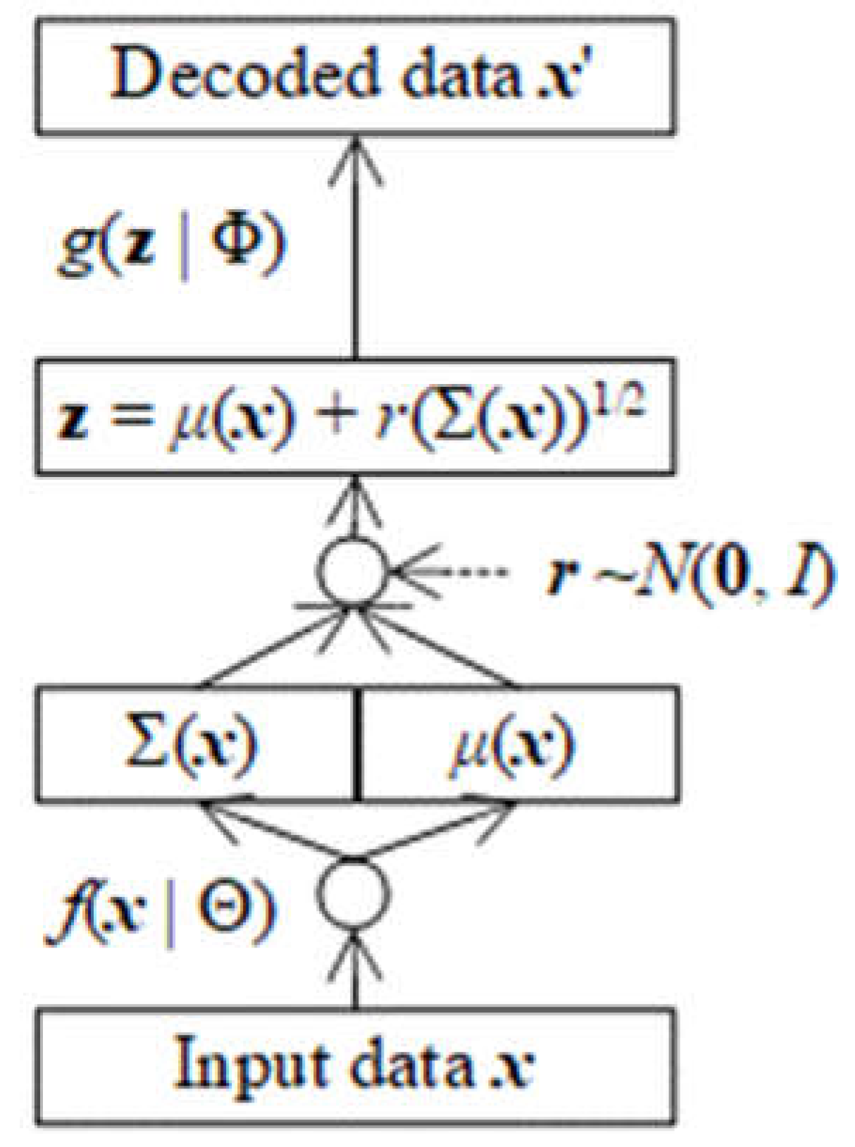
Following figure depicts VAE.

Figure 3.1. Variational Autoencoders (VAE).

Figure 3.1. Variational Autoencoders (VAE).

There is a question that how to calculate the differentials dμ(x | Θ_μ) / dΘ_μ, dσ²(x | ${\mathsf{\Theta }}_{{\mathit{\sigma }}^2}$) / d${\mathsf{\Theta }}_{{\mathit{\sigma }}^2}$, and dg(z’ | Φ) / dΦ. Indeed, it is not difficult to calculate them in context of neural network associated with backpropagation algorithm so that the last output layer as well as last neuron o of any DNN f(x | Θ) or g(z | Φ) is acted by activation function a(.) as follows:

$$\begin{gathered} a\left(o\right)=a\left({\mathit{w}}^T\mathit{i}\right) \\ o={\mathit{w}}^T\mathit{i} \end{gathered}$$

Where i is input of the last layer o and weight parameter w is a part of entire parameter Θ or Φ and hence, we need to focus on calculating differential da(o) / dw which is equivalent to any differential dμ(x | Θ_μ) / dΘ_μ, dσ²(x | ${\mathsf{\Theta }}_{{\mathit{\sigma }}^2}$) / d${\mathsf{\Theta }}_{{\mathit{\sigma }}^2}$, or dg(z’ | Φ) / dΦ so that backpropagation algorithm will solve remaining parts of entire parameter Θ or Φ.

$$\frac{da\left(o\right)}{d\mathit{w}}\cong \mathrm{a}\mathrm{n}\mathrm{y} \mathrm{d}\mathrm{i}\mathrm{f}\mathrm{f}\mathrm{e}\mathrm{r}\mathrm{e}\mathrm{n}\mathrm{t}\mathrm{i}\mathrm{a}\mathrm{l}$$

Indeed, we have:

$$\frac{da\left(o\right)}{d\mathit{w}}=\frac{da\left({\mathit{w}}^T\mathit{i}\right)}{d\mathit{w}}=\frac{da\left(o\right)}{do}{\mathit{i}}^T=a^{\prime }\left(o\right){\mathit{i}}^T$$

Note, the subscript “T” denotes transposition operator of vector and matrix in which row vector becomes column vector and vice versa. It is easy to calculate the derivative a’(o) when activation function was specified, for instance, if a(o) is sigmoid function, we have:

$$\begin{array}{l}a\left(o\right)=y=\frac{1}{1+e^{-o}}\\ a^{\prime }\left(o\right)=\frac{1}{1+e^{-o}}\left(1-\frac{1}{1+e^{-o}}\right)=a\left(o\right)\left(1-a\left(o\right)\right)=y\left(1-y\right)\end{array}$$

In practice, y is replaced by a(y) in order to prevent o from being out of space:

$$a^{\prime }\left(o\right)\cong a\left(y\right)\left(1-a\left(y\right)\right)=a\left(a\left(o\right)\right)\left(1-a\left(a\left(o\right)\right)\right)$$

As a result, we have:

$$\mathrm{a}\mathrm{n}\mathrm{y} \mathrm{d}\mathrm{i}\mathrm{f}\mathrm{f}\mathrm{e}\mathrm{r}\mathrm{e}\mathrm{n}\mathrm{t}\mathrm{i}\mathrm{a}\mathrm{l}\cong a\left(a\left(o\right)\right)\left(1-a\left(a\left(o\right)\right)\right){\mathit{i}}^T$$

For fast computation, it is possible to set the derivative a’(o) to be small enough constants like 1 such that any differential is i^T.

Given epoch D = (d⁽¹⁾ = (x⁽¹⁾, z⁽¹⁾), d⁽²⁾ = (x⁽²⁾, z⁽²⁾),…, d^(N) = (x^(N), z^(N))) implies that the epoch is created or sent by equilateral distribution 1/N but in general case, D can follow an arbitrary distribution denoted by PDF P(d), which makes the optimization problem and the SGD estimation changed a little bit by theoretical expectation given distribution P(d).

$$\begin{gathered} {\mathsf{\Theta }}^{*}=\underset{\mathsf{\Theta }}{\mathrm{armin}}E\left(\mathrm{K}\mathrm{L}\left(Q\left(\mathit{z}|\mathsf{\Theta },\mathit{x}\right)|P\left(\mathit{z}\right)\right)|P\left(\mathit{d}\right)\right) \\ {\mathsf{\Phi }}^{*}=\underset{\mathsf{\Phi }}{\mathrm{armax}}E\left(\log P\left(\mathit{x}|\mathsf{\Phi },\mathit{z}\right)|P\left(\mathit{d}\right)\right) \end{gathered}$$

Where,

$$\begin{gathered} E\left(\mathrm{K}\mathrm{L}\left(Q\left(\mathit{z}|\mathsf{\Theta },\mathit{x}\right)|P\left(\mathit{d}\right)\right)|P\left(\mathit{d}\right)\right)=\underset{\mathit{d}}{\int }\mathrm{K}\mathrm{L}\left(Q\left(\mathit{z}|\mathsf{\Theta },\mathit{x}\right)|P\left(\mathit{d}\right)\right)P\left(\mathit{d}\right)d\mathit{d} \\ E\left(\log P\left(\mathit{x}|\mathsf{\Phi },\mathit{z}\right)|P\left(\mathit{d}\right)\right)=\underset{\mathit{d}}{\int }\log P\left(\mathit{x}|\mathsf{\Phi },\mathit{z}\right)P\left(\mathit{d}\right)d\mathit{d} \end{gathered}$$

However, there is no significant change in aforementioned practical technique to estimate parameters.

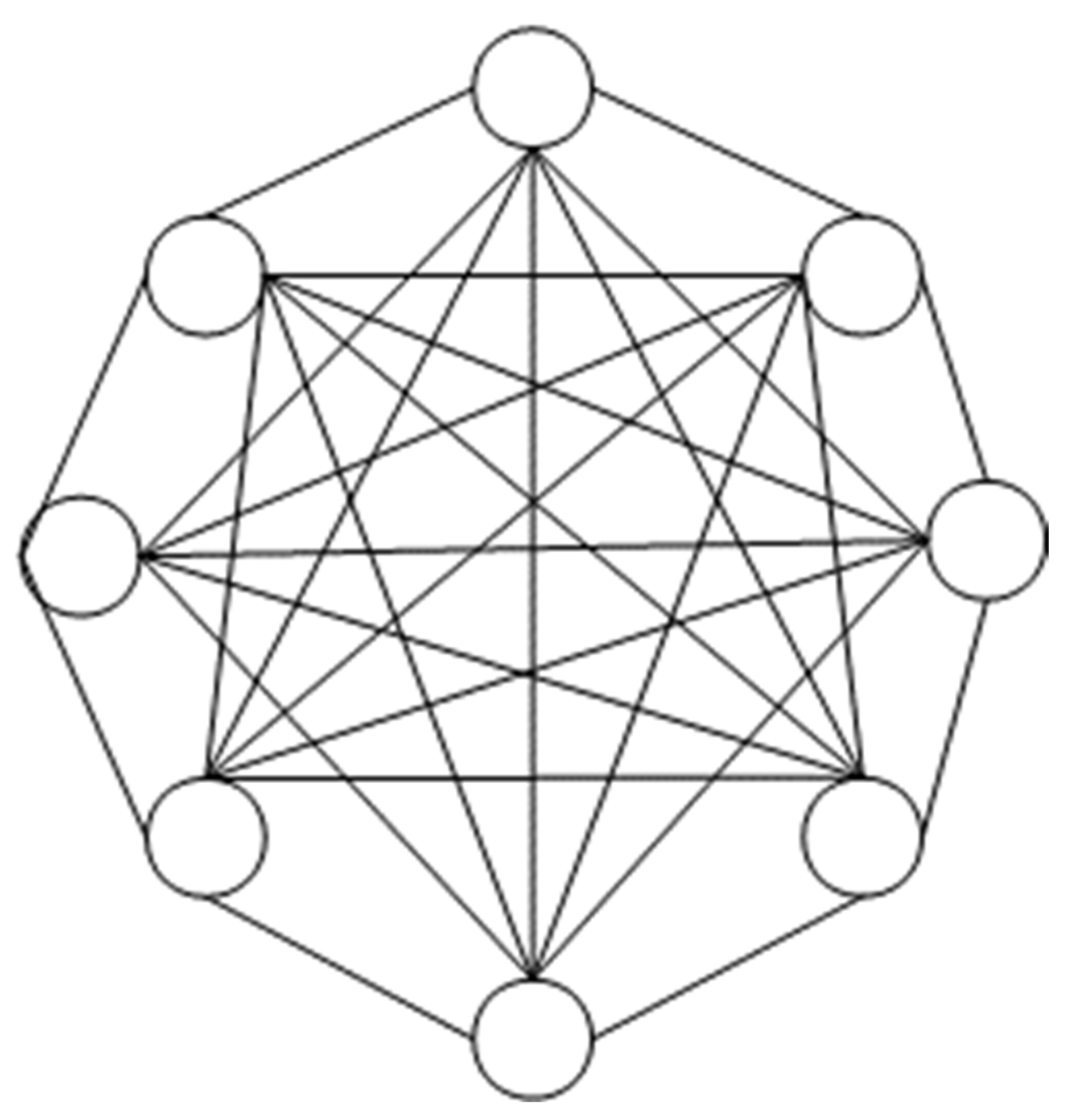
Recall that the default artificial neural network is feedforward neural network where data is fed to input layer which, in turn, is evaluated and passed across hidden layers to output layer in one-way direction, finally. However, there is an extension of neural network, which is called recurrent neural work (RNN), where an output can be turned back in order to feed on network as input. In other words, RNN has circle, which allow that output can become input. There are many kinds of RNN, for instance, long short-term memory is a case of RNN aforementioned. Boltzmann machine (Wikipedia, Boltzmann machine, 2004) is another variant of RNN, in which there is no separation of inputs from outputs. Like Hopfield network (Wikipedia, Hopfield network, 2004), every neuron (unit) in Boltzmann machine connects to all remaining neurons. In other words, Boltzmann machine applies an interesting aspect that all input neurons are output neurons too.

Figure 3.2. Topology of Hopfield network and Boltzmann machine.

Figure 3.2. Topology of Hopfield network and Boltzmann machine.

Boltzmann machine named by the name of Austrian physicist Ludwig Eduard Boltzmann, also called Sherrington-Kirkpatrick model with external field or stochastic Ising-Lenz-Little model, is a stochastic spin-glass model with an external field and classified as a Markov random filed too. For easy explanation, Boltzmann machine simulates spinning glass process or annealing metal process, in which melt glass or melt metal will be frozen or get stable at some energy and some temperature where such energy and temperature are called stable energy and stable temperature at stable state of glass. The annealing process aims to reach the stable state of metal (glass) at which time the metal is frozen. Given concrete temperature, the smaller the energy is, the more stable the metal state is. Similarly, given concrete energy, the smaller the temperature is, the more stable the metal state is. Therefore, annealing process is cooling process where probability of metal state, which is proportional to energy and temperature, follows the so-called Boltzmann distribution specified as follows:

$$P\left(s\right)=\frac{\exp \left(-\frac{E\left(s\right)}{\kappa T}\right)}{{\displaystyle {\sum }_{i=1}^M}\exp \left(-\frac{E\left(s\right)}{\kappa T}\right)}$$

(3.15)

Where P(s) is probability of current state s and E(s) is energy applied to metal at state s given temperature T while κ is Boltzmann constant and M is the number of states. Note, T can be considered as a parameter. If the denominator is constant, Boltzmann probability is approximated as follows:

$$P\left(s\right)\cong \exp \left(-\frac{E\left(s\right)}{\kappa T}\right)$$

In annealing process, if next energy is concerned by observing current energy because of successive annealing process, energy deviation or energy difference ΔE(s, s_new) between current energy E(s) and next energy E(s_new) is concerned so that Boltzmann probability derives a so-called acceptance probability P(s, s_new, T) as follows:

$$P\left(s,s_{new},T\right)=\left\{\begin{array}{l}1\mathrm{i}\mathrm{f}∆E\left(s,s_{new}\right)<0\\ \exp \left(-\frac{∆E\left(s,s_{new}\right)}{\kappa T}\right)\mathrm{o}\mathrm{t}\mathrm{h}\mathrm{e}\mathrm{r}\mathrm{w}\mathrm{i}\mathrm{s}\mathrm{e}\end{array}\right.$$

Where,

$$∆E\left(s,s_{new}\right)=E\left(s_{new}\right)-E\left(s\right)$$

Given a certain temperature T, the larger the acceptance probability is, the higher likely the annealing process stops, the higher the likelihood of stability is. In other words, acceptance probability P(s, s_new, T) decides whether or not the new state s_new is moved next in annealing process. When applied into solving optimization problem as well as learning problem, simulated annealing (SA) algorithm codes candidate solution as states. Indeed, SA is iterative process including many enough iterations where SA decreases temperature T at each iteration and then, randomize a new state s_new and calculates energy E(s_new) of the new state. Whether or not the new state (new candidate solution) s_new is based on the acceptance probability P(s, s_new, T) based on current state s, new state s_new, current temperature T. If the new candidate solution s_new is selected as current solution, SA will decrease temperature in the next iteration. Following is pseudo code of SA:

Initialize current temperature T by highest temperature T₀ as T = T₀.

Repeat

Decrease current temperature, for example, T = decrease(T).

Select a random neighbor of current state as s_new = neighbor(s).

If P(s, s_new, T) is larger than a predefined threshold then

s = s_new

End if

Until terminating conditions are met.

The terminating conditions can be that best state (solution) is reached, the current state s is good enough, the current temperature T is low enough, or the number of iterations is large enough. A usual, given a maximum iteration number K and the current iteration number k, the temperature decreasing function can be defined as follows:

$$\mathrm{d}\mathrm{e}\mathrm{c}\mathrm{r}\mathrm{e}\mathrm{a}\mathrm{s}\mathrm{e}\left(T\right)=T-\frac{k}{K}T$$

It is easy to infer that it is possible to set the initial temperature to be the maximum number of iterations as T₀ = K in practice. There is no significant change when applying SA into training Boltzmann machine where the most important problem is how to specify energy of Boltzmann machine. Fortunately, global energy of Boltzmann machine inherits from global energy of Hopfield network because Boltzmann machine is a type of Hopfield network which in turn is a variant of RNN. Suppose an entire Boltzmann machine is represented by a vector x = (x₁, x₂,…, x_n) in which each x_i is a neuron or unit. It is exact that a certain state of Boltzmann machine is represented by x which is evaluated at certain time point. It is possible to denote current state of Boltzmann machine as x instead. For convenience, the next state of Boltzmann machine is denoted x’. Energy E(x) of Boltzmann machine at state x is defined based on global energy of Hopfield network as follows (Hinton, 2007, p. 2):

$$E\left(\mathit{x}\right)=-{\displaystyle \sum _{i=1}^{n-1}}{\displaystyle \sum _{j=i+1}^n}{w}_{ij}{x}_i{x}_j-{\displaystyle \sum _{i=1}^n}{b}_i{x}_i$$

Note, w_ij is weight between neuron x_i and neuron x_j whereas b_i is bias of neuron x_i. As usual, biases b_i are considered as parameters like weights w_ij. Because there are n(n–1)/2 connections as well as n(n–1)/2 weights, the equation of energy is rewritten for convenience as follows (Wikipedia, Boltzmann machine, 2004):

$$E\left(\mathit{x}\right)=-\sum _{i<j}{w}_{ij}{x}_i{x}_j-\sum _i{b}_i{x}_i$$

(3.16)

All weights w_ij compose weight matrix W = (w_ij)_nxn whose elements on diagonal are zero. Note, W is n_xn symmetric matrix.

$$\begin{array}{l}{w}_{ij}=w_{ji},\forall i,j\\ w_{ii}=0,\forall i\mathrm{b}\mathrm{y}\mathrm{c}\mathrm{o}\mathrm{n}\mathrm{v}\mathrm{e}\mathrm{n}\mathrm{t}\mathrm{i}\mathrm{o}\mathrm{n}\end{array}$$

Every neuron x_i is evaluated by propagation rule:

$$x_i={\displaystyle \sum _{j=1,j\ne i}^n}{w}_{ij}{x}_j$$

Neurons in traditional Boltzmann machine are binary variables such that xi belongs to {0, 1} but it is extended to allow neurons x_i to belong to arbitrary real interval and so, suppose every x_i ranges in interval [0, 1] without loss of generality. Rectified Linear Unit (ReLU) function is used to ramp x_i in interval [0, 1] so as to modify the propagation rule a little bit but learning algorithm mentioned later is not changed because the first-order derivative of ReLU function within valid domain [0, 1] is 1.

$$x_i=\mathrm{R}\mathrm{e}\mathrm{L}\mathrm{U}\left({\displaystyle \sum _{j=1,j\ne i}^n}{w}_{ij}{x}_j\right)$$

Where

$$\mathrm{R}\mathrm{e}\mathrm{L}\mathrm{U}\left(x\right)=\left\{\begin{array}{r}x\mathrm{i}\mathrm{f}0\le x\le 1\\ 0\mathrm{i}\mathrm{f}x<0\\ 1\mathrm{i}\mathrm{f}x>1\end{array}\right.$$

It implies:

$$x_i=\mathrm{R}\mathrm{e}\mathrm{L}\mathrm{U}\left(x_i\right)$$

So that the propagation rule is not changed in theory:

$$x_i={\displaystyle \sum _{j=1,j\ne i}^n}{w}_{ij}{x}_j$$

Based on definition of global energy, Boltzmann probability density function (PDF) of Boltzmann machine is determined as follows:

$$P\left(\mathit{x}|\mathit{W},\mathit{b}\right)=\frac{\exp \left(-\frac{E\left(\mathit{x}|\mathit{W},\mathit{b}\right)}{\kappa T}\right)}{{\int }_{\mathit{x}}\exp \left(-\frac{E\left(\mathit{x}|\mathit{W}\right)}{\kappa T}\right)d\mathit{x}}$$

Recall that:

$$\begin{gathered} E\left(\mathit{x}|\mathit{W},\mathit{b}\right)=-\sum _{i<j}{w}_{ij}{x}_i{x}_j-\sum _i{b}_i{x}_i \\ \mathit{b}={\left(b_1,b_2,\dots ,b_n\right)}^T \end{gathered}$$

Within context of DGM, such PDF is generator likelihood whose parameter is Φ = (W, b).

$$P\left(\mathit{x}|\mathsf{\Phi }\right)=P\left(\mathit{x}|\mathit{W},\mathit{b}\right)=\frac{\exp \left(-\frac{E\left(\mathit{x}|\mathit{W},\mathit{b}\right)}{\kappa T}\right)}{{\int }_{\mathit{x}}\exp \left(-\frac{E\left(\mathit{x}|\mathit{W},\mathit{b}\right)}{\kappa T}\right)d\mathit{x}}$$

Because the denominator is constant with regard to W and b, Boltzmann PDF is approximated as follows:

$$P\left(\mathit{x}|\mathit{W},\mathit{b}\right)\cong \exp \left(-\frac{E\left(\mathit{x}|\mathit{W},\mathit{b}\right)}{\kappa T}\right)$$

(3.17)

For learning Boltzmann, maximum likelihood estimation (MLE) method (Goodfellow, Bengio, & Courville, Deep Learning, 2016, p. 655) is applied into estimating weight parameter W and bias parameter b by maximizing Boltzmann PDF with regard to w_ij and b_i.

$$\begin{gathered} w_{ij}^{*}=\underset{w_{\mathit{ij}}}{\max }P\left(\mathit{x}|\mathit{W},\mathit{b}\right) \\ {b}_i^{*}=\underset{b_i}{\max }P\left(\mathit{x}|\mathit{W},\mathit{b}\right) \end{gathered}$$

By taking natural logarithm of Boltzmann PDF, the optimization becomes easier to be solved.

$$\begin{gathered} w_{ij}^{*}=\underset{w_{\mathit{ij}}}{\max }\log P\left(\mathit{x}|\mathit{W},\mathit{b}\right) \\ {b}_i^{*}=\underset{b_i}{\max }\log P\left(\mathit{x}|\mathit{W},\mathit{b}\right) \end{gathered}$$

Where logP(x | W, b) is called Boltzmann log-likelihood or Boltzmann log-PDF.

$$\log P\left(\mathit{x}|\mathit{W},\mathit{b}\right)\cong -\frac{E\left(\mathit{x}|\mathit{W},\mathit{b}\right)}{\kappa T}$$

The first-order partial derivatives of Boltzmann log-likelihood are:

$$\begin{gathered} {\nabla }_{w_{ij}}\log P\left(\mathit{x}|\mathit{W},\mathit{b}\right)\cong \frac{\partial \log P\left(\mathit{x}|\mathit{W},\mathit{b}\right)}{\partial w_{ij}}=\frac{\partial \log E\left(\mathit{x}|\mathit{W},\mathit{b}\right)}{\partial w_{ij}}=\frac{x_i{x}_j}{\kappa T} \\ {\nabla }_{b_i}\log P\left(\mathit{x}|\mathit{W},\mathit{b}\right)\cong \frac{\partial \log P\left(\mathit{x}|\mathit{W},\mathit{b}\right)}{\partial b_i}=\frac{\partial \log E\left(\mathit{x}|\mathit{W},\mathit{b}\right)}{\partial b_i}=\frac{x_i}{\kappa T} \end{gathered}$$

As a convention, these first-order partial derivatives are called (partial) gradients. By applying stochastic gradient descent (SGD) method into estimating w_ij and b_i given Boltzmann log-likelihood, we have:

$$\begin{array}{l}{w}_{ij}=w_{ij}+\gamma {\nabla }_{w_{ij}}\log P\left(\mathit{x}|\mathit{W},\mathit{b}\right)=w_{ij}+\gamma \frac{x_i{x}_j}{\kappa T}\\ b_i=b_i+\gamma {\nabla }_{b_i}\log P\left(\mathit{x}|\mathit{W},\mathit{b}\right)=b_i+\gamma \frac{x_i}{\kappa T}\end{array}$$

(3.18)

Where 0 < γ ≤ 1 is learning rate. It is easy to recognize that the estimation equations above confirm Hebbian learning rule in which the strength of connection represented by weight is consolidated by agreement of two nodes to which the connection is attached. As a result, Boltzmann machine trained with SGD is specified as follows:

Initialize W and set k = 0.

Repeat

Data (state) x is received from some real sample, or it can be kept intact.

$$\begin{array}{l}{w}_{ij}^{\left(k+1\right)}=w_{ij}^{\left(k\right)}+\gamma \frac{x_i{x}_j}{\kappa T}\\ b_i^{\left(k+1\right)}=b_i^{\left(k\right)}+\gamma \frac{x_i}{\kappa T}\end{array}$$

Increase k = k + 1.

Until some terminating conditions are met.

Note, a terminating condition is customized, for example, parameters W and b are not changed significantly, the maximum number of iterations is reached, or Boltzmann machine gets stable. The terminating condition that Boltzmann machine gets stable receives more concerns because stability is important property of spinning glass process or annealing process that Boltzmann machine. However, checking the stability in which global energy E(x) is not changed may consume a lot of iterations. Fortunately, SA can be incorporated into SGD so as to derive a more effective estimation. Boltzmann machine trained with SGD and SA is specified as follows:

Initialize current temperature T by highest temperature T₀ as T = T₀.

Repeat

Data (state) x is received from some real sample, or it can be kept intact.

$$\begin{array}{l}{w}_{ij}^{\left(k+1\right)}=w_{ij}^{\left(k\right)}+\gamma \frac{x_i{x}_j}{\kappa T}\\ b_i^{\left(k+1\right)}=b_i^{\left(k\right)}+\gamma \frac{x_i}{\kappa T}\end{array}$$

Evaluate Boltzmann machine given current parameter W^(k+1) and b^(k+1) so as to produce a new state x’:

$$x_i^{\prime }=\mathrm{R}\mathrm{e}\mathrm{L}\mathrm{U}\left({\displaystyle \sum _{j=1,j\ne i}^n}{w}_{ij}^{\left(k+1\right)}{x}_j\right),\mathrm{f}\mathrm{o}\mathrm{r}\mathrm{a}\mathrm{l}\mathrm{l}{x}_i^{\prime }\mathrm{n}\mathrm{o}\mathrm{t}\mathrm{f}\mathrm{r}\mathrm{o}\mathrm{m}\mathrm{r}\mathrm{e}\mathrm{a}\mathrm{l}\mathrm{s}\mathrm{a}\mathrm{m}\mathrm{p}\mathrm{l}\mathrm{e}$$

If P(x, x’, T | W^(k+1), b^(k+1) is larger than a predefined threshold then

x = x’

Decrease current temperature, for example, T = decrease(T).

End if

Increase k = k + 1.

Until terminating conditions are met.

The terminating conditions can be that best state (x’) is reached, the current state x is good enough, or the current temperature T is low enough. These terminating conditions reflect the stable state of Boltzmann machine. A usual, given a maximum iteration number K and the current iteration number k, the temperature decreasing function can be defined as follows:

$$\mathrm{d}\mathrm{e}\mathrm{c}\mathrm{r}\mathrm{e}\mathrm{a}\mathrm{s}\mathrm{e}\left(T\right)=T-\frac{k}{K}T$$

Of course, the acceptance probability is:

$$P\left(\mathit{x},{\mathit{x}}^{\prime },T|\mathit{W},\mathit{b}\right)=\left\{\begin{array}{l}1\mathrm{i}\mathrm{f}∆E\left(\mathit{x},{\mathit{x}}^{\prime }|\mathit{W},\mathit{b}\right)<0\\ \exp \left(-\frac{∆E\left(\mathit{x},{\mathit{x}}^{\prime }|\mathit{W},\mathit{b}\right)}{\kappa T}\right)\mathrm{o}\mathrm{t}\mathrm{h}\mathrm{e}\mathrm{r}\mathrm{w}\mathrm{i}\mathrm{s}\mathrm{e}\end{array}\right.$$

(3.19)

Where,

$$∆E\left(\mathit{x},{\mathit{x}}^{\prime }|\mathit{W},\mathit{b}\right)=E\left({\mathit{x}}^{\prime }|\mathit{W},\mathit{b}\right)-E\left(\mathit{x}|\mathit{W},\mathit{b}\right)$$

There is a so-called restricted Boltzmann machine (RBM) in which neurons are separated into two groups such as input group denoted x_z and hidden group denoted x_x.

$$\mathit{x}={\left({\mathit{x}}_z,{\mathit{x}}_x\right)}^T$$

The training algorithm by incorporation of SA and SGD is not changed except that there is neither connection between input neurons and input neurons nor connection between hidden neurons and hidden neurons. In other words, all connections are made between input group and hidden group, for instance, suppose cardinality of input group is k then, the number of connections is k(n – k). Therefore, the two groups are considered layers such as input layer and hidden layer. Of course, both layers are output layers because connections in Boltzmann machine are two-direction connections whereas feed-forward neural network accepts only one-direction connections. RBM is trained faster than traditional Boltzmann machine because its number of connections is smaller. Moreover, it is clear to apply RBM into DGM because generator function in DGM x = g(z | Φ) is modeled by RBM whose input is input group x_z and whose output is output group x_x such as x_x = g(x_z | W, b) where x_x is calculated by evaluating RBM given input x_z.

$${\mathit{x}}_x=g\left({\mathit{x}}_z|\mathit{W},\mathit{b}\right)\stackrel{\scriptscriptstyle\mathrm{def}}{=}\mathrm{e}\mathrm{v}\mathrm{a}\mathrm{l}\mathrm{u}\mathrm{a}\mathrm{t}\mathrm{e}\mathrm{R}\mathrm{B}\mathrm{M}\mathrm{a}\mathrm{t}{\mathit{x}}_z\mathrm{t}\mathrm{o}\mathrm{p}\mathrm{r}\mathrm{o}\mathrm{d}\mathrm{u}\mathrm{c}\mathrm{e}{\mathit{x}}_x$$

The reason that the RBM approach for DGM is classified into approximate density DGM is that generator likelihood P(x | W, b) is defined indirectly based on the energy E(x | W, b). Of course, x_z is randomized such that x_x is generated data.

4. Implicit Density DGM

According to implicit density approach, DGMs do not specify explicitly generator PDF P(x | Φ, z), which does not means that such PDF is not existent but it is simple that such PDF is not concerned. Note, PDF is abbreviation of probability density function.

Recall that there are two problems related to construct a DGM: 1) how to define likelihood or error to train generator DNN g(z | Φ) and 2) how to define tractable PDF P(z) which implies the way to randomize z. The second problem relates to assert qualification of random data z’ and hence, the second problem is stated as qualification problem of how to qualify random data. However, it is essential that the qualification problem aims to improve generator DNN g(z | Φ) because g(z | Φ) translate intractable z into tractable x. Generative Adversarial Network (GAN) developed by Goodfellow et al. (Goodfellow, et al., 2014) aims to reinforcing quality of generator DNN g(z | Φ) = x’ ≈ x by adding a so-called discriminator which is a discrimination function d(x | Ψ): x → [0, 1] from concerned data x or x’ to range [0, 1] in which d(x | Ψ) can distinguish fake data from real data. In other words, the larger result the discriminator d(x’ | Ψ) derives, the more realistic the generated data x’ is. Obviously, discriminator d(x | Ψ) is implemented by a DNN whose weights are Ψ called discriminator parameter with note that this discriminator DNN has only one output neuron denoted d₀.

$$d:R^m\to \left[\mathrm{0,1}\right]\mathrm{s}\mathrm{u}\mathrm{c}\mathrm{h}\mathrm{t}\mathrm{h}\mathrm{a}\mathrm{t}{d}_0=d\left(\mathit{x}|\mathsf{\Psi }\right)\mathrm{w}\mathrm{h}\mathrm{e}\mathrm{r}\mathrm{e}{d}_0\in \left[\mathrm{0,1}\right],\mathit{x}\in X\subseteq R^m$$

(4.1)

Actually, the task of discriminator d(x | Ψ) is classification task with regard to class d₀ belonging to interval [0, 1]. GAN does not establish explicitly PDFs of generator g(z | Φ) and discriminator d(x | Ψ) such as P(x | Φ, z) and P(d₀ | Ψ, x) and hence, GAN does not define explicitly and separately likelihoods / errors of g(z | Φ) and d(x | Ψ) too. Indeed, GAN instead unifies optimization constraints of g(z | Φ) and d(x | Ψ) into a target function l(Φ, Ψ | x, z).

$$l\left(\mathsf{\Phi },\mathsf{\Psi }|\mathit{x},\mathit{z}\right)=\log \left(d\left(\mathit{x}|\mathsf{\Psi }\right)\right)+\log \left(1-d\left(g\left(\mathit{z}|\mathsf{\Phi }\right)|\mathsf{\Psi }\right)\right)$$

(4.2)

Indeed, target function l(Φ, Ψ | x, z) is error function and so it is called loss function in literature. As a result, GAN tries to optimize dually generator parameter Φ and discriminator parameter Ψ so that optimal estimate Φ^* and optimal estimate Ψ^* are minimizer and maximizer of loss function l(Φ, Ψ | x, z) with expectation that Nash equilibrium will be achieved at the saddle point (Φ^*, Ψ^*) with note that loss function l(Φ, Ψ | x, z) is function of Φ and Ψ given data x and z.

$$\begin{array}{l}{\mathsf{\Phi }}^{*}=\underset{\mathsf{\Phi }}{\mathrm{argmin}}l\left(\mathsf{\Phi },{\mathsf{\Psi }}^{*}|\mathit{x},\mathit{z}\right)=\underset{\mathsf{\Phi }}{\mathrm{argmin}}\log \left(1-d\left(g\left(\mathit{z}|\mathsf{\Phi }\right)|{\mathsf{\Psi }}^{*}\right)\right)\\ {\mathsf{\Psi }}^{*}=\underset{\mathsf{\Psi }}{\mathrm{argmax}}l\left({\mathsf{\Phi }}^{*},\mathsf{\Psi }|\mathit{x},\mathit{z}\right)=\underset{\mathsf{\Psi }}{\mathrm{argmax}}\left(\log \left(d\left(\mathit{x}|\mathsf{\Psi }\right)\right)+\log \left(1-d\left(g\left(\mathit{z}|{\mathsf{\Phi }}^{*}\right)|\mathsf{\Psi }\right)\right)\right)\end{array}$$

(4.3)

This is min-max problem in game theory (Goodfellow, et al., 2014):

$$\underset{\mathsf{\Phi }}{\min }\underset{\mathsf{\Psi }}{\max }l\left(\mathsf{\Phi },\mathsf{\Psi }|\mathit{x},\mathit{z}\right)$$

Which results estimation equation according to stochastic gradient descent (SGD) method:

$$\begin{gathered} \mathsf{\Phi }=\mathsf{\Phi }-\gamma {\nabla }_{\mathsf{\Phi }}l\left(\mathsf{\Phi },{\mathsf{\Psi }}^{*}|\mathit{x},\mathit{z}\right) \\ \mathsf{\Psi }=\mathsf{\Psi }+\gamma {\nabla }_{\mathsf{\Psi }}l\left({\mathsf{\Phi }}^{*},\mathsf{\Psi }|\mathit{x},\mathit{z}\right) \end{gathered}$$

Where γ is learning rate. Recall that SGD, which is an iterative process, pushes candidate solution at each iteration along the direction which is opposite to gradient of target function for minimization or has the same direction to gradient of target function for maximization with note that the step length is represented by learning rate. Note, ∇_Φl(Φ, Ψ^* | x, z) is gradient of loss function l(Φ, Ψ^* | x, z) fixed Ψ^* with regard to generator parameter Φ and ∇_Ψl(Φ^*, Ψ | x, z) is gradient of loss function l(Φ^*, Ψ | x, z) fixed Φ^* with regard to discriminator parameter Ψ as follows:

$$\begin{array}{l}{\nabla }_{\mathsf{\Phi }}l\left(\mathsf{\Phi },{\mathsf{\Psi }}^{*}|\mathit{x},\mathit{z}\right)=\frac{dl\left(\mathsf{\Phi },{\mathsf{\Psi }}^{*}|\mathit{x},\mathit{z}\right)}{d\mathsf{\Phi }}=\frac{\partial \log \left(1-d\left(g\left(\mathit{z}|\mathsf{\Phi }\right)|{\mathsf{\Psi }}^{*}\right)\right)}{\partial \mathsf{\Phi }}\\ {\nabla }_{\mathsf{\Psi }}l\left({\mathsf{\Phi }}^{*},\mathsf{\Psi }|\mathit{x},\mathit{z}\right)=\frac{dl\left({\mathsf{\Phi }}^{*},\mathsf{\Psi }|\mathit{x},\mathit{z}\right)}{d\mathsf{\Psi }}=\frac{\partial \left(\log \left(d\left(\mathit{x}|\mathsf{\Psi }\right)\right)+\log \left(1-d\left(g\left(\mathit{z}|{\mathsf{\Phi }}^{*}\right)|\mathsf{\Psi }\right)\right)\right)}{\partial \mathsf{\Psi }}\end{array}$$

Therefore, the estimation equation is rewritten as follows:

$$\begin{array}{l}\mathsf{\Phi }=\mathsf{\Phi }-\gamma {\nabla }_{\mathsf{\Phi }}\log \left(1-d\left(g\left(\mathit{z}|\mathsf{\Phi }\right)|{\mathsf{\Psi }}^{*}\right)\right)\\ \mathsf{\Psi }=\mathsf{\Psi }+\gamma {\nabla }_{\mathsf{\Psi }}\left(\log \left(d\left(\mathit{x}|\mathsf{\Psi }\right)\right)+\log \left(1-d\left(g\left(\mathit{z}|{\mathsf{\Phi }}^{*}\right)|\mathsf{\Psi }\right)\right)\right)\end{array}$$

(4.4)

According to equations above, real data x aims to maximize discriminator d(x | Ψ) and in opposite, generated data x’ = g(z | Φ) aims to minimize discriminator d(x’ | Ψ). Although both GAN and VAE use two DNNs for data generation but the underlying theory of GAN is slightly more succinct than VAE because there is no requirement of specifying probabilistic distribution P(z) of tractable z. As a convention, the gradient ∇_Φ(log(1 – d(g(z | Φ) | Ψ^*))) related to generator parameter Θ is called generator gradient and the gradient ∇_Ψ(log(d(x | Ψ)) + log(1 – d(g(z | Φ^*) | Ψ))) related to discriminator parameter Θ is called discriminator gradient.

Given epoch of size N is denoted as D = ((x⁽¹⁾, z⁽¹⁾), (x⁽²⁾, z⁽²⁾),…, (x^(N), z^(N))), the estimation equations of Φ and Ψ are extended exactly as epoch estimation at every iteration of SGD:

$$\begin{array}{l}{\mathsf{\Phi }}^{\left(k+1\right)}={\mathsf{\Phi }}^{\left(k\right)}-\gamma {\nabla }_{\mathsf{\Phi }}\frac{1}{N}{\displaystyle \sum _{i=1}^N}\log \left(1-d\left(g\left({\mathit{z}}^{\left(i\right)}|{\mathsf{\Phi }}^{\left(k\right)}\right)|{\mathsf{\Psi }}^{\left(k\right)}\right)\right)\\ {\mathsf{\Psi }}^{\left(k+1\right)}={\mathsf{\Psi }}^{\left(k\right)}+\gamma {\nabla }_{\mathsf{\Psi }}\frac{1}{N}{\displaystyle \sum _{i=1}^N}\left(\log \left(d\left({\mathit{x}}^{\left(i\right)}|{\mathsf{\Psi }}^{\left(k\right)}\right)\right)+\log \left(1-d\left(g\left({\mathit{z}}^{\left(i\right)}|{\mathsf{\Phi }}^{\left(k\right)}\right)|{\mathsf{\Psi }}^{\left(k\right)}\right)\right)\right)\end{array}$$

As a result, GAN trained with SGD is specified as follows:

Initialize Φ and Ψ and set k = 0.

Repeat

Sampling epoch X = (x⁽¹⁾, x⁽²⁾,…, x^(N)) or receiving epoch X from big data / data stream.

Randomize random epoch Z = (z⁽¹⁾, z⁽²⁾,…, z^(N)) from standard normal distribution P(z) = $\mathcal{N}$(z | 0, I) with mean 0 and identity covariance matrix I.

$$\begin{array}{l}{\mathsf{\Phi }}^{\left(k+1\right)}={\mathsf{\Phi }}^{\left(k\right)}-\gamma {\nabla }_{\mathsf{\Phi }}\frac{1}{N}{\displaystyle \sum _{i=1}^N}\log \left(1-d\left(g\left({\mathit{z}}^{\left(i\right)}|{\mathsf{\Phi }}^{\left(k\right)}\right)|{\mathsf{\Psi }}^{\left(k\right)}\right)\right)\\ {\mathsf{\Psi }}^{\left(k+1\right)}={\mathsf{\Psi }}^{\left(k\right)}+\gamma {\nabla }_{\mathsf{\Psi }}\frac{1}{N}{\displaystyle \sum _{i=1}^N}\left(\log \left(d\left({\mathit{x}}^{\left(i\right)}|{\mathsf{\Psi }}^{\left(k\right)}\right)\right)+\log \left(1-d\left(g\left({\mathit{z}}^{\left(i\right)}|{\mathsf{\Phi }}^{\left(k\right)}\right)|{\mathsf{\Psi }}^{\left(k\right)}\right)\right)\right)\end{array}$$

Increase k = k + 1.

Until some terminating conditions are met.

Note, a terminating condition is customized, for example, parameters Φ and Ψ are not changed significantly or there is no more coming epoch X. Moreover, the index k indicates time point as well as iteration of SGD.

Recall that the estimation equations of generator parameter Φ and discriminator parameter Ψ are:

$$\begin{array}{l}\mathsf{\Phi }=\mathsf{\Phi }-\gamma {\nabla }_{\mathsf{\Phi }}\log \left(1-d\left(g\left(\mathit{z}|\mathsf{\Phi }\right)|{\mathsf{\Psi }}^{*}\right)\right)\\ \mathsf{\Psi }=\mathsf{\Psi }+\gamma {\nabla }_{\mathsf{\Psi }}\left(\log \left(d\left(\mathit{x}|\mathsf{\Psi }\right)\right)+\log \left(1-d\left(g\left(\mathit{z}|{\mathsf{\Phi }}^{*}\right)|\mathsf{\Psi }\right)\right)\right)\end{array}$$

It is necessary to calculate generator gradient and discriminator gradient. Indeed, we have:

$$\begin{array}{l}{\nabla }_{\mathsf{\Phi }}\log \left(1-d\left(g\left(\mathit{z}|\mathsf{\Phi }\right)|{\mathsf{\Psi }}^{*}\right)\right)=\frac{\partial \log \left(1-d\left(g\left(\mathit{z}|\mathsf{\Phi }\right)|{\mathsf{\Psi }}^{*}\right)\right)}{\partial \mathsf{\Phi }}=-\frac{\partial d\left(g\left(\mathit{z}|\mathsf{\Phi }\right)|{\mathsf{\Psi }}^{*}\right)/\partial \mathsf{\Phi }}{1-d\left(g\left(\mathit{z}|\mathsf{\Phi }\right)|{\mathsf{\Psi }}^{*}\right)}\\ {\nabla }_{\mathsf{\Psi }}\left(\log \left(d\left(\mathit{x}|\mathsf{\Psi }\right)\right)+\log \left(1-d\left(g\left(\mathit{z}|{\mathsf{\Phi }}^{*}\right)|\mathsf{\Psi }\right)\right)\right)\\ =\frac{\partial \left(\log \left(d\left(\mathit{x}|\mathsf{\Psi }\right)\right)+\log \left(1-d\left(g\left(\mathit{z}|{\mathsf{\Phi }}^{*}\right)|\mathsf{\Psi }\right)\right)\right)}{\partial \mathsf{\Psi }}\\ =\frac{\partial d\left(\mathit{x}|\mathsf{\Psi }\right)/\partial \mathsf{\Psi }}{d\left(\mathit{x}|\mathsf{\Psi }\right)}-\frac{\partial d\left(g\left(\mathit{z}|{\mathsf{\Phi }}^{*}\right)|\mathsf{\Psi }\right)/\partial \mathsf{\Psi }}{1-d\left(g\left(\mathit{z}|{\mathsf{\Phi }}^{*}\right)|\mathsf{\Psi }\right)}\end{array}$$

Where ∂d(.) / ∂Φ and ∂d(.) / ∂Ψ denotes differentials of discriminator function with regard to Φ and Ψ, respectively.

Given epoch of size N is denoted as D = ((x⁽¹⁾, z⁽¹⁾), (x⁽²⁾, z⁽²⁾),…, (x^(N), z^(N))), the estimation equations of Φ and Ψ are extended exactly as epoch estimation at every iteration of SGD:

$$\begin{array}{l}{\mathsf{\Phi }}^{\left(k+1\right)}={\mathsf{\Phi }}^{\left(k\right)}+\gamma \frac{1}{N}{\displaystyle \sum _{i=1}^N}\frac{\partial d\left(g\left({\mathit{z}}^{\left(i\right)}|{\mathsf{\Phi }}^{\left(k\right)}\right)|{\mathsf{\Psi }}^{\left(k\right)}\right)/\partial \mathsf{\Phi }}{1-d\left(g\left({\mathit{z}}^{\left(i\right)}|{\mathsf{\Phi }}^{\left(k\right)}\right)|{\mathsf{\Psi }}^{\left(k\right)}\right)}\\ {\mathsf{\Psi }}^{\left(k+1\right)}={\mathsf{\Psi }}^{\left(k\right)}+\gamma \frac{1}{N}{\displaystyle \sum _{i=1}^N}\left(\frac{\partial d\left({\mathit{x}}^{\left(i\right)}|{\mathsf{\Psi }}^{\left(k\right)}\right)/\partial \mathsf{\Psi }}{d\left({\mathit{x}}^{\left(i\right)}|{\mathsf{\Psi }}^{\left(k\right)}\right)}-\frac{\partial d\left(g\left({\mathit{z}}^{\left(i\right)}|{\mathsf{\Phi }}^{\left(k\right)}\right)|{\mathsf{\Psi }}^{\left(k\right)}\right)/\partial \mathsf{\Psi }}{1-d\left(g\left({\mathit{z}}^{\left(i\right)}|{\mathsf{\Phi }}^{\left(k\right)}\right)|{\mathsf{\Psi }}^{\left(k\right)}\right)}\right)\end{array}$$

(4.5)

As a result, GAN trained with SGD is specified as follows:

Initialize Φ and Ψ and set k = 0.

Repeat

Sampling epoch X = (x⁽¹⁾, x⁽²⁾,…, x^(N)) or receiving epoch X from big data / data stream.

Randomize random epoch Z = (z⁽¹⁾, z⁽²⁾,…, z^(N)) from standard normal distribution P(z) = $\mathcal{N}$(z | 0, I) with mean 0 and identity covariance matrix I.

$$\begin{array}{l}{\mathsf{\Phi }}^{\left(k+1\right)}={\mathsf{\Phi }}^{\left(k\right)}+\gamma \frac{1}{N}{\displaystyle \sum _{i=1}^N}\frac{\partial d\left(g\left({\mathit{z}}^{\left(i\right)}|{\mathsf{\Phi }}^{\left(k\right)}\right)|{\mathsf{\Psi }}^{\left(k\right)}\right)/\partial \mathsf{\Phi }}{1-d\left(g\left({\mathit{z}}^{\left(i\right)}|{\mathsf{\Phi }}^{\left(k\right)}\right)|{\mathsf{\Psi }}^{\left(k\right)}\right)}\\ {\mathsf{\Psi }}^{\left(k+1\right)}={\mathsf{\Psi }}^{\left(k\right)}+\gamma \frac{1}{N}{\displaystyle \sum _{i=1}^N}\left(\frac{\partial d\left({\mathit{x}}^{\left(i\right)}|{\mathsf{\Psi }}^{\left(k\right)}\right)/\partial \mathsf{\Psi }}{d\left({\mathit{x}}^{\left(i\right)}|{\mathsf{\Psi }}^{\left(k\right)}\right)}-\frac{\partial d\left(g\left({\mathit{z}}^{\left(i\right)}|{\mathsf{\Phi }}^{\left(k\right)}\right)|{\mathsf{\Psi }}^{\left(k\right)}\right)/\partial \mathsf{\Psi }}{1-d\left(g\left({\mathit{z}}^{\left(i\right)}|{\mathsf{\Phi }}^{\left(k\right)}\right)|{\mathsf{\Psi }}^{\left(k\right)}\right)}\right)\end{array}$$

Increase k = k + 1.

Until some terminating conditions are met.

Note, a terminating condition is customized, for example, parameters Φ and Ψ are not changed significantly or there is no more coming epoch X. Moreover, the index k indicates time point as well as iteration of SGD.

Following figure depicts GAN.

Figure 4.1. Generative Adversarial Network (GAN).

Figure 4.1. Generative Adversarial Network (GAN).

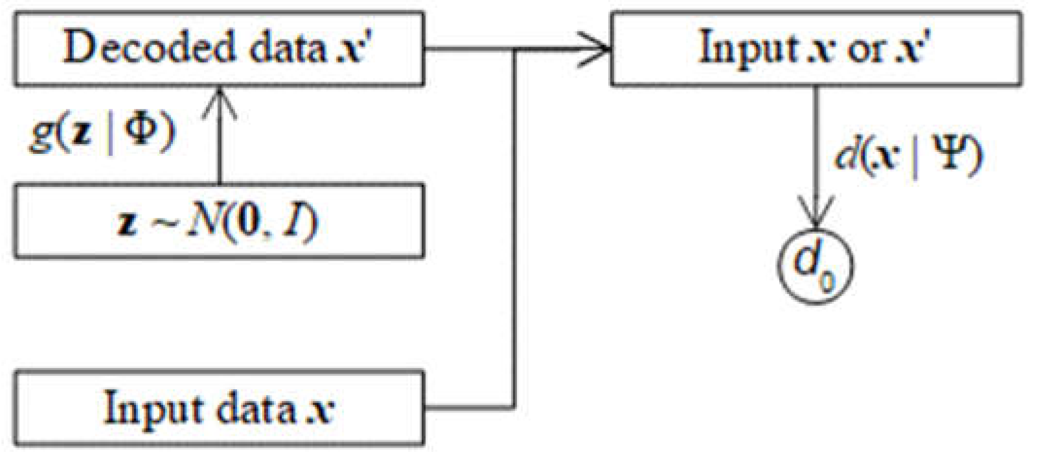
There is a question that how to calculate the differentials ∂d(.) / ∂Φ and ∂d(.) / ∂Ψ. Indeed, it is not difficult to calculate them in context of neural network associated with backpropagation algorithm so that the last output layer as well as last neuron o of any DNN f(x | Θ) or g(z | Φ) is acted by activation function a(.) as follows:

$$\begin{gathered} a\left(o\right)=a\left({\mathit{w}}^T\mathit{i}\right) \\ o={\mathit{w}}^T\mathit{i} \end{gathered}$$

Where i is input of the last layer o and weight parameter w is a part of entire parameter Φ or Ψ and hence, we need to focus on calculating differential da(o) / dw which is equivalent to any differential ∂d(.) / ∂Φ or ∂d(.) / ∂Ψ so that backpropagation algorithm will solve remaining parts of entire parameter Φ or Ψ.

$$\frac{da\left(o\right)}{d\mathit{w}}\cong \mathrm{a}\mathrm{n}\mathrm{y} \mathrm{d}\mathrm{i}\mathrm{f}\mathrm{f}\mathrm{e}\mathrm{r}\mathrm{e}\mathrm{n}\mathrm{t}\mathrm{i}\mathrm{a}\mathrm{l}$$

Indeed, we have:

$$\frac{da\left(o\right)}{d\mathit{w}}=\frac{da\left({\mathit{w}}^T\mathit{i}\right)}{d\mathit{w}}=\frac{da\left(o\right)}{do}{\mathit{i}}^T=a^{\prime }\left(o\right){\mathit{i}}^T$$

Note, the subscript “T” denotes transposition operator of vector and matrix in which row vector becomes column vector and vice versa. It is easy to calculate the derivative a’(o) when activation function was specified, for instance, if a(o) is sigmoid function, we have:

$$\begin{array}{l}a\left(o\right)=y=\frac{1}{1+e^{-o}}\\ a^{\prime }\left(o\right)=\frac{1}{1+e^{-o}}\left(1-\frac{1}{1+e^{-o}}\right)=a\left(o\right)\left(1-a\left(o\right)\right)=y\left(1-y\right)\end{array}$$

In practice, y is replaced by a(y) in order to prevent o from being out of space:

$$a^{\prime }\left(o\right)\cong a\left(y\right)\left(1-a\left(y\right)\right)=a\left(a\left(o\right)\right)\left(1-a\left(a\left(o\right)\right)\right)$$

As a result, we have:

$$\mathrm{a}\mathrm{n}\mathrm{y} \mathrm{d}\mathrm{i}\mathrm{f}\mathrm{f}\mathrm{e}\mathrm{r}\mathrm{e}\mathrm{n}\mathrm{t}\mathrm{i}\mathrm{a}\mathrm{l}\cong a\left(a\left(o\right)\right)\left(1-a\left(a\left(o\right)\right)\right){\mathit{i}}^T$$

For fast computation, it is possible to set the derivative a’(o) to be small enough constants like 1 such that any differential is i^T.

Given epoch D = (d⁽¹⁾ = (x⁽¹⁾, z⁽¹⁾), d⁽²⁾ = (x⁽²⁾, z⁽²⁾),…, d^(N) = (x^(N), z^(N))) implies that the epoch is created or sent by equilateral distribution 1/N but in general case, D can follow an arbitrary distribution denoted by PDF P(d), which makes loss function l(Φ, Ψ) changed a little bit by theoretical expectation given distribution P(d).

$$l\left(\mathsf{\Phi },\mathsf{\Psi }\right)=\underset{\mathit{d}}{\int }\left(\log \left(d\left(\mathit{x}|\mathsf{\Psi }\right)\right)+\log \left(1-d\left(g\left(\mathit{z}|\mathsf{\Phi }\right)|\mathsf{\Psi }\right)\right)\right)d\mathit{d}$$

Suppose x and z distribute separately as P(x) and Q(z) such that P(x) is called original data PDF and Q(z) is called generated data PDF, we have:

$$l\left(\mathsf{\Phi },\mathsf{\Psi }\right)=\underset{\mathit{x}}{\int }P\left(\mathit{x}\right)\log \left(d\left(\mathit{x}|\mathsf{\Psi }\right)\right)d\mathit{x}+\underset{\mathit{z}}{\int }Q\left(\mathit{z}\right)\log \left(1-d\left(g\left(\mathit{z}|\mathsf{\Phi }\right)|\mathsf{\Psi }\right)\right)d\mathit{z}$$

(4.6)

Although there is no significant change in aforementioned practical technique to estimate parameters, it is necessary to research original data PDF P(x) and generated data PDF Q(z) as well as expectation form of loss function l(Φ, Ψ) so as to prove convergence of GAN. Recall that the min-max problem is:

$$\underset{\mathsf{\Phi }}{\min }\underset{\mathsf{\Psi }}{\max }l\left(\mathsf{\Phi },\mathsf{\Psi }\right)$$

That is:

$$\begin{gathered} {\mathsf{\Phi }}^{*}=\underset{\mathsf{\Phi }}{\mathrm{argmin}}l\left(\mathsf{\Phi },{\mathsf{\Psi }}^{*}\right) \\ {\mathsf{\Psi }}^{*}=\underset{\mathsf{\Psi }}{\mathrm{argmax}}l\left({\mathsf{\Phi }}^{*},\mathsf{\Psi }\right) \end{gathered}$$

The convergence of GAN is equivalent to the convergence of this min-max problem. In other words, Goodfellow et al. (Goodfellow, et al., 2014) proved the existence of global optimal value l^* such that min-max problem approach l^* as follows:

$$l^{*}=l\left({\mathsf{\Phi }}^{*},{\mathsf{\Psi }}^{*}\right)=\underset{\mathsf{\Phi }}{\min }l\left(\mathsf{\Phi },{\mathsf{\Psi }}^{*}\right)=\underset{\mathsf{\Phi }}{\min }\underset{\mathsf{\Psi }}{\max }l\left(\mathsf{\Phi },\mathsf{\Psi }\right)$$

(4.7)

Because z is generated by distribution Q(z) and g(z | Φ) is valuated as x as g(z | Φ) = x, loss function l(Φ, Ψ) is rewritten by changing variable (Goodfellow, et al., 2014, p. 5).

$$\begin{array}{l}l\left(\mathsf{\Phi },\mathsf{\Psi }\right)=\underset{\mathit{x}}{\int }P\left(\mathit{x}\right)\log \left(d\left(\mathit{x}|\mathsf{\Psi }\right)\right)d\mathit{x}+\underset{\mathit{x}}{\int }Q\left(\mathit{x}\right)\log \left(1-d\left(\mathit{x}|\mathsf{\Psi }\right)\right)d\mathit{x}\\ =\underset{\mathit{x}}{\int }\left(P\left(\mathit{x}\right)\log \left(d\left(\mathit{x}|\mathsf{\Psi }\right)\right)+Q\left(\mathit{x}\right)\log \left(1-d\left(\mathit{x}|\mathsf{\Psi }\right)\right)\right)d\mathit{x}\end{array}$$

In mathematical literature, function alog(y) + blog(1–y) gets maximal at maximizer y = a/(a+b) such that:

$$d\left(\mathit{x}|{\mathsf{\Psi }}^{*}\right)=\frac{P\left(\mathit{x}\right)}{P\left(\mathit{x}\right)+Q\left(\mathit{x}\right)}$$

Therefore, we have (Goodfellow, et al., 2014, p. 5):

$$\begin{array}{l}\underset{\mathsf{\Psi }}{\max }l\left(\mathsf{\Phi },\mathsf{\Psi }\right)=l\left(\mathsf{\Phi },{\mathsf{\Psi }}^{*}\right)=\underset{\mathit{x}}{\int }\left(P\left(\mathit{x}\right)\log \left(\frac{P\left(\mathit{x}\right)}{P\left(\mathit{x}\right)+Q\left(\mathit{x}\right)}\right)+Q\left(\mathit{x}\right)\log \left(\frac{Q\left(\mathit{x}\right)}{P\left(\mathit{x}\right)+Q\left(\mathit{x}\right)}\right)\right)d\mathit{x}\\ =\\ =\underset{\mathit{x}}{\int }P\left(\mathit{x}\right)\log \left(\frac{2P\left(\mathit{x}\right)}{P\left(\mathit{x}\right)+Q\left(\mathit{x}\right)}\right)d\mathit{x}+\underset{\mathit{x}}{\int }Q\left(\mathit{x}\right)\log \left(\frac{2Q\left(\mathit{x}\right)}{P\left(\mathit{x}\right)+Q\left(\mathit{x}\right)}\right)d\mathit{x}-\mathrm{l}\mathrm{o}\mathrm{g}4\\ =\mathrm{K}\mathrm{L}\left(P\left(\mathit{x}\right)|\frac{P\left(\mathit{x}\right)+Q\left(\mathit{x}\right)}{2}\right)+\mathrm{K}\mathrm{L}\left(Q\left(\mathit{x}\right)|\frac{P\left(\mathit{x}\right)+Q\left(\mathit{x}\right)}{2}\right)-\mathrm{l}\mathrm{o}\mathrm{g}4\end{array}$$

Where KL(.) denotes Kullback-Leibler divergence of two distributions. The sum of two KL divergences above is a so-called Jensen-Shannon divergence of original data distribution P(x) and generated data distribution Q(z), denoted JS(P(x) | Q(x)). Therefore, we have (Goodfellow, et al., 2014, p. 5):

$$\underset{\mathsf{\Psi }}{\max }l\left(\mathsf{\Phi },\mathsf{\Psi }\right)=l\left(\mathsf{\Phi },{\mathsf{\Psi }}^{*}\right)=\mathrm{J}\mathrm{S}\left(P\left(\mathit{x}\right)|Q\left(\mathit{x}\right)\right)-\mathrm{l}\mathrm{o}\mathrm{g}4$$

Because Jensen-Shannon divergence is always nonnegative, we have (Goodfellow, et al., 2014, p. 5):

$$\underset{\mathsf{\Psi }}{\max }l\left(\mathsf{\Phi },\mathsf{\Psi }\right)=l\left(\mathsf{\Phi },{\mathsf{\Psi }}^{*}\right)\ge -\mathrm{l}\mathrm{o}\mathrm{g}4$$

The sign “=” occurs because Jensen-Shannon divergence is zero if the two distributions are equal, for instance, P(x) = Q(x). Therefore, l(Φ, Ψ^*) has maximal value –log4. In other words, we have:

$$l^{*}=l\left({\mathsf{\Phi }}^{*},{\mathsf{\Psi }}^{*}\right)=\underset{\mathsf{\Phi }}{\min }\underset{\mathsf{\Psi }}{\max }l\left(\mathsf{\Phi },\mathsf{\Psi }\right)=-\mathrm{l}\mathrm{o}\mathrm{g}4$$

(4.8)

Due to the existence of global optimal value l^* = –log4, the convergence of GAN is asserted.

5. Conclusions

Recall that there are three main approaches for constructing deep generative model (DGM) such as tractable density DGM, approximate density DGM, and implicit density DGM. When skimming these approaches, it is easy to recognize that applied statistical problems such as probability distribution and parameter estimation are often mentioned but the effectiveness of a deep generative model is also dependent on how to structure the deep neural network (DNN) and how to train such network. Anyhow data generation function called generator is always defined by DNN in DGM. Backpropagation (BP) algorithm associated with stochastic gradient descent (SGD) method is focused as typical example in this research but there are some more effective training algorithms. Essential, training DNN generator is unsupervised learning task because there is no data class in DGM although generating data distribution (distribution of tractable data z) is often assumed to follow normal distribution whereas BP belongs to supervised learning algorithm. This is the reason that the two problems of constructing DGM are 1) how to train generator DNN g(z | Φ) and 2) how to qualify such training task which often relates to another optimization task or another training task so that the qualification task tries to attach supervised learning BP to unsupervised learning mechanism. For instance, PixelRNN allows output data becomes input data by recurrent neural network, VAE applies Kullback-Leibler divergence into forming data distribution as implicit data class, and GAN issues target function with expectation of Nash equilibrium. Essentially, these mechanisms make the exchange or transformation between supervised learning and unsupervised learning, which plays the role of a hinge for creating the DNN generator.

One of problems issued by BP is the zero derivative problem when SGD cannot improve parameters after some large enough iteration because the gradient (derivative) approaches zero at that time. In other words, SGD may not converge even though there is a large enough number of iterations. Moreover, basic DGM approaches mentioned here require a continuous data provision for training DNN, which consumes more resources than reinforcement learning.

References

- Doersch, C. (2016, January 3). Tutorial on Variational Autoencoders. arXiv preprint. Retrieved from https://arxiv.org/abs/1606.05908.
- Goodfellow, I., Bengio, Y., & Courville, A. (2016). Deep Learning. Cambridge, Massachusetts, US: The MIT Press. Retrieved from https://www.deeplearningbook.org/.
- Goodfellow, I., Pouget-Abadie, J., Mirza, M., Xu, B., Warde-Farley, D., Ozair, S., . . . Bengio, Y. (2014). Generative Adversarial Nets. In Z. Ghahramani, M. Welling, C. Cortes, N. Lawrence, & K. Weinberger (Ed.), Advances in Neural Information Processing Systems 27 (NIPS 2014). 27. Montreal: NeurIPS. Retrieved from https://proceedings.neurips.cc/paper_files/paper/2014/file/5ca3e9b122f61f8f06494c97b1afccf3-Paper.pdf.
- Hardle, W., & Simar, L. (2013). Applied Multivariate Statistical Analysis. Berlin, Germany: Research Data Center, School of Business and Economics, Humboldt University.
- Hinton, G. E. (2007). Boltzmann machine. Brain Corporation, 2(5), 1668. [CrossRef]
- Kingma, D. P., & Welling, M. (2022, December 10). Auto-Encoding Variational Bayes. arXiv Preprint, 1-14. [CrossRef]
- Nguyen, L. (2015). Matrix Analysis and Calculus (1st ed.). (C. Evans, Ed.) Hanoi, Vietnam: Lambert Academic Publishing. Retrieved March 3, 2014, from https://www.shuyuan.sg/store/gb/book/matrix-analysis-and-calculus/isbn/978-3-659-69400-4.
- Nguyen, L. (2023). Tutorial on artificial neural network. Loc Nguyen’s Academic Network. Open Science Framework (OSF). doi:https://osf.io/k8syc.
- Oord, A. v., Kalchbrenner, N., & Kavukcuoglu, K. (2016, August 19). Pixel Recurrent Neural Networks. arXiv preprint, 1-11. [CrossRef]
- Oussidi, A., & Elhassouny, A. (2018). Deep generative models: Survey. 2018 International Conference on Intelligent Systems and Computer Vision (ISCV). Fez, Morocco: IEEE. [CrossRef]
- Ruthotto, L., & Haber, E. (2021, April 12). An Introduction to Deep Generative Modeling. arXiv preprint. [CrossRef]
- Theis, L., & Bethge, M. (2015, September 18). Generative Image Modeling Using Spatial LSTMs. In C. Cortes, N. Lawrence, D. Lee, M. Sugiyama, & R. Garnett (Ed.), Advances in Neural Information Processing Systems 28 (NIPS 2015). 28, pp. 1-9. Montreal: NeurIPS. [CrossRef]
- Wikipedia. (2004, November 13). Boltzmann machine. (Wikimedia Foundation) Retrieved from Wikipedia website: https://en.wikipedia.org/wiki/Boltzmann_machine.
- Wikipedia. (2004, November 15). Hopfield network. (Wikimedia Foundation) Retrieved from Wikipedia website: https://en.wikipedia.org/wiki/Hopfield_network.
- Wikipedia. (2004, February 13). Kullback-Leibler divergence. (Wikimedia Foundation) Retrieved from Wikipedia website: https://en.wikipedia.org/wiki/Kullback%E2%80%93Leibler_divergence.
- Wikipedia. (2005, April 7). Recurrent neural network. (Wikimedia Foundation) Retrieved from Wikipedia website: https://en.wikipedia.org/wiki/Recurrent_neural_network.
- Wikipedia. (2006, February 9). Jensen-Shannon divergence. (Wikimedia Foundation) Retrieved from Wikipedia: https://en.wikipedia.org/wiki/Jensen%E2%80%93Shannon_divergence.
- Wikipedia. (2007, April 16). Long short-term memory. (Wikimedia Foundation) Retrieved from Wikipedia website: https://en.wikipedia.org/wiki/Long_short-term_memory.
Disclaimer/Publisher’s Note: The statements, opinions and data contained in all publications are solely those of the individual author(s) and contributor(s) and not of MDPI and/or the editor(s). MDPI and/or the editor(s) disclaim responsibility for any injury to people or property resulting from any ideas, methods, instructions or products referred to in the content. |
© 2024 by the authors. Licensee MDPI, Basel, Switzerland. This article is an open access article distributed under the terms and conditions of the Creative Commons Attribution (CC BY) license (http://creativecommons.org/licenses/by/4.0/).
Copyright: This open access article is published under a Creative Commons CC BY 4.0 license, which permit the free download, distribution, and reuse, provided that the author and preprint are cited in any reuse.