Submitted:
06 May 2024
Posted:
09 May 2024
You are already at the latest version
Abstract
The laser host materials undergo relatively small changes in their intrinsic properties due to various sources during an experiment. These sources are often related to temperature change or applied stress, which may cause change in optical properties of the material under study.
Consequently, the crystal experiences an optical anisotropy, which may affect the final outcome of the experiments. One way to reduce probable noises is to predict the change in optical properties with respect to load. To predict the changing pattern of the refractive index in a crystal, one needs to know both the elastic and photoelastic constants of the material. In this study, we utilized density functional perturbation theory (DFPT) to extract the photoelastic tensor of Y$_2$SiO$_5$ and Eu-doped Y$_2$SiO$_5$ crystals. Using the photoelastic and elastic constants calculated, a Finite Element (FE) model was developed, which allowed us to apply load and then post-process the results. This methodology enabled us to observe the variation in refractive index ($n$), and consequently, the shift in the resonance frequency of the cavity.
The results obtained were in agreement with experimental measurements, falling within a 3\% discrepancy across a temperature range spanning from cryogenic to room temperature. This correlation suggests the feasibility of using the current workflow as a predictive tool for evaluating variations in refractive indices over a specific interval.
Keywords:
Refractive index
; resonance frequency
; DFT
; optical path length
; elasto-optic constants
1. Introduction
An optical cavity, like a laser resonator, has certain frequencies at which it resonantly enhances the electromagnetic field. These resonant frequencies are determined by the condition that the optical path length of the cavity (the distance that light travels inside the cavity) be an integer multiple of the wavelength of the light. This is necessary for the light wave to constructively interfere with itself after each round trip in the cavity, and it’s what allows a laser, for example, to generate a strong, coherent beam of light. Mathematically, the condition for resonance is given by [1]:
where m is the mode number (number of round trips in the cavity) is an integer, is the wavelength, L is the physical length of the cavity and nis the refractive index. Now, if the optical path length changes - either because the physical length of the cavity changes, or because the refractive index of the medium changes (due to a temperature change) - then the other side of the equation above changes. To maintain equality, the wavelength of the light must also change. But the frequency (f) and wavelength of light are related by the speed of light (c):
So if the wavelength changes while the speed of light remains constant, the frequency must also change. Hence, a change in the optical path length of a cavity results in a shift in the resonant frequencies of the cavity.
In practical terms, this concept implies that by exercising meticulous control over the length of an optical cavity, for instance, by delicately adjusting the position of one of the mirrors in a laser system, we gain the ability to fine-tune the frequency at which the cavity resonates. A crucial outcome of this mechanism is the potential to optimize the signal-to-noise ratio. This essentially entails boosting the desired information, or the signal, in the output, while simultaneously minimizing any undesired interference or noise, thereby enhancing the overall quality and accuracy of the laser’s performance.
For instance, the resonance frequency of a cavity is used to stabilize a laser’s frequency [2]. This is achieved by aligning the laser’s frequency to the resonance frequency of the cavity, which means transferring the stability of the cavity to the laser [3]. Hence, the reference cavity acts as an optical resonator that serves as a frequency reference in optical frequency standards [4]. In turn, an ultra-high frequency stability laser is an essential part of an optical atomic clocks [5], and a myriad of optical precision measurements [6,7].
Given the importance of understanding the factors influencing the physical length of a cavity or the refractive index of a medium, it is essential to examine the phenomena that contribute to these variations. In this work, however, the analysis will primarily concentrate on changes in the refractive index as a result of an external load. The photoelastic effect, which describes changes in the optical properties of a material under mechanical deformation, is employed to examine this alteration. Nevertheless, the applicability of the photoelastic effect is dependent on the availability of the elasto-optic tensor elements. These elements are instrumental in discerning the optical path difference across the crystal.
Furthermore, since the photoelastic properties of a material can be significantly influenced by its electronic structure, and the fact that impurities within a crystal lattice can modify the distribution of stress across the material that can subsequently lead to shifts in the material’s photoelastic behavior. We investigate two cases: a pure case and a doped case.
Our initial step involves the calculation of photoelastic constants for both pure Yttrium Orthosilicate (YSO), denoted as YSiO, and Europium-doped YSO. This process is executed through the application of Density Functional Perturbation Theory (DFPT) [8]. Subsequently, leveraging the elastic constants calculated in our previous study [9], we have developed a Finite Element (FE) model. This model allows us to examine the impact of mechanical loads, specifically temperature and stress, on the refractive index of both pure and Eu-doped YSO, which in turn allows us to observe the shift in resonance frequency of the cavity.
YSiO
YSO, is a dielectric material with biaxial anisotropy, and its refractive index at various frequencies is well-documented [10]. It is a monoclinic biaxial crystal that belongs to the C2/c () space group [11], where Rare-Earth (RE) ions can substitute for the Y ions. It is a well-known host material for RE ions, and it’s used extensively in optical research. Given the monoclinic nature of the crystal, it necessitates four distinct dielectric functions, denoted as , to accurately portray the material’s interaction with light. Here, represents frequency. These functions are particularly crucial in the wavelength region where the material exhibits transparency [12,13]. The principal values of the dielectric functions are unequal and they are ordered as << [12]. The off-diagonal, , is a small value but it is non-zero.
The YSO crystal structure is characterized by three distinct, unequal crystallographic axes, labeled as a, b, and c. These axes have respective lengths of 14.51 Å, 6.81 Å, and 10.51 Å. Notably, axis b is perpendicular to both a and c, while the angle between axes a and c is denoted by [14]. Apart from the primary crystallographic axes, YSO is further defined by its optical axes: D, D, and b [14,15]. The relationship between these optical axes and the crystallographic axes is captured in Figure 2 [14].
In experiments involving YSO crystal, the optical beam is typically directed to propagate along the crystallographic b-axis of the crystal and polarized along the D axis since this setup provides the largest absorption [16]. Moreover, the b-axis aligns with the optic axis of the crystal, thereby making it an axis of symmetry. This property can contribute to more predictable and desirable outcomes in optical experiments.
2. Theory & Method
2.1. Theoretical Background
The elasto-optic effect illustrates the change in the optical properties of a material under the influence of stress. The indices of refraction of an unstressed material can be described by Maxwell’s equations, but it will lead to impractical long equations. To simplify, an ellipsoid as an analogy is used to express the variation of refractive indices. This ellipsoid is known as indicatrix [17], and it is identified by the following relation:
where , , are the principal axes, and , , and are their corresponding refractive indices. The coefficients of this ellipsoid are the components of the relative dielectric impermeability tensor, , at optical frequencies, so the general form of indicatrix can be written as:
This way the small change of refractive index produced by stress can be traced by a change in the shape, size, and orientation of the indicatrix [11], and the changes in the coefficients of indicatrix, , under applied stress, or strain , is given as:
where , and are fourth-rank elasto-optic and piezo-optic tensors. The left-hand side of the above equation can be rewritten as:
where and are the dielectric impermeability tensor before and after the applied stress [11]. Moreover, as the principal components of B tensor are simply the inverse of the dielectric tensor [11] and the relation between refractive index and dielectric tensor is = , Equation 6 can be rewritten as:
This means the knowledge of applied stress along with piezo-optic coefficients would show us how much the refractive index would change with respect to applied stress.
The B is actually a 3x3 matrix in which it can be reduced with respect to the symmetry of the crystal, and take the form that is similar to the dielectric tensor in Equation 3.
In the same way, the which is normally a 6x6 matrix can be reduced to its corresponding monoclinic form [18], which allows us to rewrite the Equation 6 as:
The resultant matrix multiplication becomes:
The matrix on the left-hand side of the above equation can be rewritten to its original matrix form using index change notation as 23 and 32 → 4, 31 and 13 → 5, 12 and 21 → 6 [11]. Finally, the monoclinic symmetry of the matrix was considered to attain its final form.
we can now obtain the resultant matrix, which contains the refractive index after applied pressure.
Finally, we reach the elements that correspond to the principal axes of the dielectric impermeability tensor,
in which the corresponding refractive indices of the principal axes after the applied pressure is:
2.2. Computational Method
The ab-initio calculations are carried out using the CRYSTAL [19], and VASP [20]. The CRYSTAL code uses linear combinations of Gaussian Type Functions (GTF) as basis sets to construct the fictitious wave functions. The exchange and correlation part of Hamiltonian were treated based on PBE0 [21] method, and PBE [22]. An effective core potential atom-centered GTF basis set of triple- valence quality, augmented by a polarization function (TZVP), is adopted for each element in the system. The truncation criteria for electronic integrals are controlled by five thresholds, which are set to 8, 8, 8, 10, and 20. Last but not least, the sampling of the reciprocal space was conducted using a shrinking factor of 4, and the convergence criterion on total energy was set to Hartree.
The VASP calculations were conducted with the following setup. The cut-off energy was set to, 520 eV, while the k-point set for the unit cell was selected to be 4×8×6. The convergence threshold was set to 1× eV, and the force criterion for geometry optimization was 0.00001 eV/Å.
The extraction of piezo-optic and elasto-optic elements is conducted by applying a sequence of deformation matrices to the relaxed standard unit cell of YSO. These deformation matrices can be found in the Appendix. Following each deformation, we calculate the dielectric constant of the deformed unit cell. Subsequently, by employing a manipulated version of Equation 6, the piezo-optic and elasto-optic elements are derived.
For the finite element analysis, a 3D model was created and four pressure loads and a thermal load were analyzed – uniaxial load in two different directions, biaxial load and hydrostatic pressure. This is achieved by utilizing the pre-calculated elastic constants from our previous study [9], as well as thermal coefficient constants courtesy of Sun et al [23] and Marion et al. [24]. The schematic view of the crystal setup in ABAQUS is shown in Figure 3, a rectangular crystal with dimensions length of 5 mm, height of 4 mm, and depth of 1 mm.
Due to the symmetry of the crystal, only one-fourth of the geometry was modeled and symmetry conditions were imposed into the two symmetry axes D and D assumed. The mesh is refined to 0.5 mm to describe a reliable stress profile. The element type used in the crystal is an 8-node thermally coupled linear brick element.
Following the application of temperature and stress to the model, we extract the resulting stress matrices for further post-processing. This entails multiplying by the piezo-optic tensor to obtain the affected impermeability matrix. The refractive index influenced by stress is then obtained by performing the manipulations that were detailed in the preceding section.
3. Result & Discussion
The data presented in Table 1 illustrates both the experimentally obtained and the computationally determined values for pure YSO. It also includes the refractive index values for YSO doped with Eu. Upon a preliminary comparison of the experimental and calculated values using the PBE functional, an overestimation was observed. In response to this discrepancy, the hybrid PBE0 approach was employed, resulting in improved congruity between experimental and theoretical results for pure YSO. Our results have the largest discrepancy with results provided by Weber [25]. So, we made a comparison with those results. The discrepancies for n, n, and n are 1.25%, 1.22%, and 1.77%, respectively, which shows the overall agreement between our theoretical findings and the experimental results.
When comparing the refractive indices of doped and undoped materials, a small but noticeable increase is observed across all principal axes. The largest divergence occurs in the D-direction, with a relative increase of 0.0114. In contrast, the smallest change is detected along the b-axis, with a discrepancy of only 0.0071. While it is difficult to draw definitive conclusions from a single data point, this trend suggests that impurities may increase the relative permittivity, leading to an increase in the refractive index. This is consistent with the previous findings [26,27], who reported that RE-doping can increase the dielectric constant of the host material, although their study did not focus on YSO.
Table 2 demonstrates the elastic constants calculated in our previous work. This table is introduced with dual objectives. Firstly, these values contribute to establishing the Finite Element (FE) model in ABAQUS. Secondly, these values help evaluate the accuracy of the photoelastic constants, which represent changes in the optical properties of a material under mechanical deformation. There is a lack of experimental data for both pure and doped versions of the YSO compound. However, the accuracy of the photoelastic constants can still be probed by comparing the difference between the elastic constants and refractive indices of the pure and doped compounds.
Table 3 displays the piezo-optic constants for both pure and Eu-doped YSO that are obtained based on the work of Erba et al. [30,31]. The choice of functional for our calculations was based on the values of refractive indices presented in Table 1. Specifically, we continued with the same type of functional, PBE0 since functional provided values closest to the experimental observations. In an ideal scenario, our methodology’s accuracy would be confirmed by comparing our calculated photoelastic constants with experimental equivalents. However, for both pure and Eu-doped YSO, such data is currently unavailable. As a workaround, we validated our calculated piezo-optic and inherent elasto-optic constants via their application in FEM simulations. In these simulations, we applied loads and post-processed the results using the calculated piezo-optic constants. If the refractive index resulting from these simulations, after the load application, aligns with the available experimental refractive index under similar conditions, we can assert that our piezo-optic constants are correctly determined.
To perform a comparative analysis, we utilized the measured values of relative permittivity from the study by Carvalho et al. [10]. These values denote the real permittivity of pure YSO crystal against varying temperatures with the uncertainty of below 0.26% [10]. As the YSO crystal is a biaxial dielectric material with known refractive indices at optical frequencies, its permittivity plays a crucial role in this comparison. Following this, we commenced with the application of thermal stress on the YSO crystal. The temperature model employed is a thermomechanical one, where any temperature exceeding 0 K incites a mechanical load on the crystal, thereby inducing stress on the unit cell. This stress is then post-processed via the application of piezo-optic constants. This step assists in obtaining the refractive indices influenced by the stress, thereby allowing us to perform an analysis of the material’s behavior under thermal conditions.
To observe the orientation-dependent of the n versus temperature, we can refer to Figure 4. Here we have plotted the variation of n in principal axes for both measured and calculated data. It is clear that the calculated model follows the right trend with increasing temperature.
However in all directions, we observe the quadratic type curve for the measured data and the linear type curve for the calculated data. This can be proved by comparing the fitted polynomials for the measured and calculated curves, where we find the corresponding coefficients are as follows: a = 1.3×10, b = 2.4×10, c = 1.7(4908) for the measured curve and a = 3.1×10, b = -2.712×10, c = 1.7(5770) for the calculated curve. These findings assert the linearity of the calculated data as the coefficient of x being a, is in order of 10 while the coefficient a for the measured data is in order of 10. The main reason behind the linearity of the calculated result may be the extracted photoelastic constants that are a result of Pockel’s effect [31], which is intrinsically a linear effect. It should be added that Pockels’ effect is essentially a term allocated to linear electro-optic effect [11]. Since there is no specific term for linear elasto-optic effect, we have extended the definition of Pockels’ effect to linear elasto-optic effect. Therefore, the quadratic trait of the calculated curve might be achieved if the extracted photoelastic constants were obtained with nonlinear traits known as Kerr effect [11]. Again, the Kerr effect is a term coined for non-linear electro-optic effect but we extend its definition to cover nonlinear elasto-optic effects as well.
Our calculated results can be further substantiated through a direct comparison with empirical data sourced from Carvalho et al. [10]. A side-by-side representation of the corresponding values for our measurements and calculations is presented in Table 5, with data points spanning from 6 to 296 K. The table shows consistent precision in both the measured and calculated data, as indicated by the four decimal places. The error percentages vary slightly across different temperatures, except for a sharp increase at 500K and 1000K, demonstrating numerical stability. The data is also accurate and reliable, as both measured and calculated values have four significant digits, which allows for a precise comparison. The choice of four significant digits is justified by the sensitivity of the refractive index to small deviations, which would affect the frequency significantly. For the D orientation, the deviation in our point-to-point comparison is minimal. Additionally, the percentage of error remains unchanged across the entire temperature range. For the sake of specificity, the maximum errors at D, b, and D stand at 0.49, 1.84, and 2.78 respectively. The parentheses around the value of n after the decimal point are only added to help the reader see how n changes along the temperature interval.
It’s important to highlight that for direction b and D, the error seems to amplify faster as temperature increases. To better understand the magnitude of error at higher temperatures, we utilize a curve that has been fitted to predict the error beyond room temperature. The last three rows of Table 5 display the measured values of the refractive indices—calculated using the fitted curves—in comparison with the computed data. A significant rise in error is discernible at the 500 and 1000 K points. It is crucial to recognize that the operating temperature for some RE-activated phosphors is typically at or slightly above room temperature. For instance, the temperature required for laser stabilization is at cryogenic levels [2,4], while for common phosphor applications, like lighting LEDs, the operating temperature tends to be near or just above room temperature [32]. Thus, we can assert that the predictions of the model align with experimental findings and are applicable for practical uses. At least, this is the case for applications up to and smaller than room temperature.
After constructing and verifying the ability of the model to produce reasonable results, we proceeded to investigate the changes in refractive indices with respect to the temperature of Eu-doped YSO. The Eu concentration for the doped system was maintained at 6.25% to remain consistent with our previous study [9], and it should be mentioned that the doping is performed only for site 1 of YSO. The results of these computations are detailed in Table 6. Consistent with the findings for the undoped system, the doped system also exhibits a linear pattern in its refractive indices.
Based on these calculated refractive indices, one can track the shift of resonance frequency for pure YSO and Eu-doped YSO medium. Figure 5 shows the shift of the frequency with respect to temperature. As the figure shows, the trend of the curves in both cases (pure and doped) are linear and have an increasing trend in which the value of the principal axes keeps the same order of magnitude D>b>D.
Next, our study involves assessing the impact of applying compressive and tensile loads directly to the crystal, specifically focusing on the variation of nin different orientations. We will reapply pressure to the crystal during the FE simulation, which previously provided us with the stress tensor. This tensor will then be subjected to further post-processing via the piezo-optic tensor to derive the fluctuation of refractive indices about the applied load.
Figure 5 illustrates how n changes with the applied load in D, D, and DD directions, as well as hydrostatic pressure. From previous observations, we can anticipate a linear trend, as the piezo-optic constants were derived based on Pockels’ effect. The focal points in this instance are the slope of the hydrostatic pressure and the close approximation of the D and DD. As you can see in all figures the maximum magnitude of change is related to hydrostatic pressure, and the curves corresponding to D and DD are almost overlapping which might be explained due to the larger magnitude of nin D direction.
Interestingly, the doped crystal (Figure 6) exhibits similar behavior to the pure system. To discern the differences between the pure and doped systems, we have contrasted the rates of change in resonance frequencies for both systems, as tabulated in Table 7. The table demonstrates that doping results in a steeper slope - as far as the magnitude of the slope is concerned - across all orientations. Therefore, one could deduce that doping accelerates the rate of change in refractive indices, and by extension, the resonance frequency. Regrettably, there are no such data available to corroborate this for YSO, although a study conducted by Soharab et al. [33] analyzed the refractive index versus Nd concentration in GdVO, which seems to support the increasing trend of refractive indices with dopant concentration.
4. Conclusion
In this study, a multi-scale modeling workflow was developed and we have managed to calculate the refractive index with respect to temperature, , of both pure and Eu-doped YSO. To achieve this the piezo-optic constants were extracted with the application of DFPT, and the calculated constant was validated using the measured value of the for the pure YSO. For the selected temperature interval (6 - 296 K) the maximum error between calculated and measured values was at 2.78% in D direction. The main discrepancy between the developed model and the measured data is the shape of the curves, where measured data possess a quadratic shape while the calculated data have a linear shape. As we mentioned in the result section, this must be because we have extracted the piezo-optic constant based on Pockels’ effect which is a linear approach in its origin. So, to decrease the discrepancy between calculated and measured data non-linear effects known as Kerr’s effect must be added to the process of piezo-optic extraction. Nevertheless, the workflow produces reasonable results for at least the selected temperature interval. The produced results presented in Table 5 are important as they enable the estimation of thermo-optic coefficients, which is crucial for the optimization and design of the optical cavity.
Using the piezo-optic post-processing method, we successfully observed variations in refractive indices for different applied loads and their respective frequency shifts. Our observations indicate that hydrostatic pressure induces the most significant variation in the refractive index. Furthermore, a linear relationship exists between the applied load and the change in refractive index. Doping amplifies the variation magnitude, regardless of its orientation or magnitude of the applied load. Thus, it can be inferred that an increase in impurity concentration amplifies the variation in nand subsequently affects the resonance frequency.
The accuracy of the results with respect to experimental and the applicability of this approach for other host materials and dopants and the ease of the workflow suggest that the current approach has the potential to be a straightforward alternative for the tedious experimental measurement. This is especially the case for low-symmetry materials such as YSO. Nevertheless, the main purpose of this work was to propose an approach to examine variation of the refractive indices for RE-doped YSO in which we believe we have shown it is possible to do so to a large degree.
Acknowledgments
The authors are grateful to Matheus Amarante Machado and Jimmy Bisou for their assistance in FEM simulations and the post-processing stage. This work is supported by the Knut & Alice Wallenberg Foundation through grant no.: KAW-2016.0081. The simulations were performed using computational resources provided by the Swedish National Infrastructure for Computing (SNIC) at UPPMAX, Uppsala University, the NSC, Linköping University, and the PDC, Royal Institute of Technology.
Conflicts of Interest
The authors declare no conflicts of interest.
Appendix A
References
- A. Konijnenberg, A. Adam, and P. Urbach, BSc Optics (TU Delft Open, 2021).
- M. J. Thorpe, L. Rippe, T. M. Fortier, M. S. Kirchner, and T. Rosenband, “Frequency stabilization to 6 × 10-16 via spectral-hole burning,” Nature Photonics 5, 688–693 (2011).
- J. Millo, D. V. Magalhães, C. Mandache, Y. Le Coq, E. M. L. English, P. G. Westergaard, J. Lodewyck, S. Bize, P. Lemonde, and G. Santarelli, “Ultrastable lasers based on vibration insensitive cavities,” Phys. Rev. A 79, 053829 (2009).
- N. Galland, N. Lučić, B. Fang, S. Zhang, R. Le Targat, A. Ferrier, P. Goldner, S. Seidelin, and Y. Le Coq, “Mechanical tunability of an ultranarrow spectral feature of a Rare-Earth-doped crystal via uniaxial stress,” Phys. Rev. Appl. 13, 044022 (2020).
- A. D. Ludlow, M. M. Boyd, J. Ye, E. Peik, and P. O. Schmidt, “Optical atomic clocks,” Rev. Mod. Phys. 87, 637–701 (2015).
- J. M. Hogan and M. A. Kasevich, “Atom-interferometric gravitational-wave detection using heterodyne laser links,” Phys. Rev. A 94, 033632 (2016).
- P. Ghelfi, F. Laghezza, F. Scotti, G. Serafino, A. Capria, S. Pinna, D. Onori, C. Porzi, M. Scaffardi, A. Malacarne et al., “A fully photonics-based coherent radar system,” Nature 507, 341–345 (2014).
- X. Gonze, “Adiabatic density-functional perturbation theory,” Phys. Rev. A 52, 1096–1114 (1995).
- A. Mirzai, A. Ahadi, S. Melin, and P. Olsson, “First-principle investigation of doping effects on mechanical and thermodynamic properties of Y2SiO5,” Mechanics of Materials 154, 103739 (2021).
- N. Carvalho, J.-M. Le Floch, J. Krupka, and M. Tobar, “Multi-mode technique for the determination of the biaxial Y2SiO5 permittivity tensor from 300 to 6 k,” Applied Physics Letters 106 (2015).
- J. F. Nye, Physical properties of crystals: Their representation by tensors and matrices (Oxford University, 1985).
- J. Jellison, Gerald E., E. D. Specht, L. A. Boatner, D. J. Singh, and C. L. Melcher, “Spectroscopic refractive indices of monoclinic single crystal and ceramic lutetium oxyorthosilicate from 200 to 850 nm,” Journal of Applied Physics 112 (2012). 063524.
- G. E. Jellison, M. A. McGuire, L. A. Boatner, J. D. Budai, E. D. Specht, and D. J. Singh, “Spectroscopic dielectric tensor of monoclinic crystals: CdWO4,” Phys. Rev. B 84, 195439 (2011).
- G. Erdei, N. Berze, Á. Péter, B. Játékos, and E. Lorincz, “Refractive index measurement of Cerium-doped LuxY2- xSiO5 single crystal,” Optical Materials 34, 781–785 (2012).
- C. Li, C. Wyon, and R. Moncorge, “Spectroscopic properties and fluorescence dynamics of Er3+ and Yb3+ in Y2SiO5,” IEEE journal of quantum electronics 28, 1209–1221 (1992).
- A. Ferrier, B. Tumino, and P. Goldner, “Variations in the oscillator strength of the 7f0→5d0 transition in Eu3+:Y2SiO5 single crystals,” Journal of Luminescence 170, 406–410 (2016). SI: Lanthanide spectroscopy.
- E. Hecht, Optik (De Gruyter, Berlin, Boston, 2018).
- T. S. Narasimhamurty, Photoelastic and electro-optic properties of crystals (Springer Science & Business Media, 2012).
- R. Dovesi, A. Erba, R. Orlando, C. M. Zicovich-Wilson, B. Civalleri, L. Maschio, M. Rérat, S. Casassa, J. Baima, S. Salustro et al., “Quantum-mechanical condensed matter simulations with crystal,” Wiley Interdisciplinary Reviews: Computational Molecular Science 8, e1360 (2018).
- G. Kresse and J. Furthmüller, “Efficiency of ab-initio total energy calculations for metals and semiconductors using a plane-wave basis set,” Computational Materials Science 6, 15 – 50 (1996).
- C. Adamo and V. Barone, “Toward reliable density functional methods without adjustable parameters: The PBE0 model,” The Journal of chemical physics 110, 6158–6170 (1999).
- J. P. Perdew, K. Burke, and M. Ernzerhof, “Generalized gradient approximation made simple,” Phys. Rev. Lett. 77, 3865–3868 (1996).
- Z. Sun, M. Li, and Y. Zhou, “Thermal properties of single-phase Y2SiO5,” Journal of the European Ceramic Society 29, 551–557 (2009).
- J. Marion and R. Beach, “Thermophysical properties of Y2SiO5 (YOS),” (1990).
- M. J. Weber, Handbook of optical materials, vol. 19 (CRC, 2002).
- Y. Chen, D. Zhang, Z. Peng, M. Yuan, and X. Ji, “Review of research on the rare-earth doped piezoelectric materials,” Frontiers in Materials 8 (2021).
- X. Wang, X. Shi, R. Zhang, Y. Shi, Y. Liang, B. Zhang, H. Li, S. Hu, K. Yu, Y. Hu et al., “Effect of Co doping on microstructure, dielectric, and energy storage properties of bczt ceramics,” Journal of Materials Science: Materials in Electronics 33, 20399–20412 (2022).
- E. T. Miyazono, “Nanophotonic resonators for optical quantum memories based on rare-earth-doped materials,” Ph.D. thesis, California Institute of Technology (2017).
- Y. Luo, J. Wang, J. Wang, J. Li, and Z. Hu, “Theoretical predictions on elastic stiffness and intrinsic thermal conductivities of Yttrium Silicates,” Journal of the American Ceramic Society 97, 945–951 (2014).
- A. Erba and R. Dovesi, “Photoelasticity of crystals from theoretical simulations,” Phys. Rev. B 88, 045121 (2013).
- A. Erba, M. T. Ruggiero, T. M. Korter, and R. Dovesi, “Piezo-optic tensor of crystals from quantum-mechanical calculations,” The Journal of Chemical Physics 143, 144504 (2015).
- I. Ayoub, U. Mushtaq, N. Hussain, S. Rubab, R. Sehgal, H. C. Swart, and V. Kumar, “8 - rare-earth-activated phosphors for led applications,” in Rare-Earth-Activated Phosphors, V. Dubey, N. Dubey, M. M. Domańska, M. Jayasimhadri, and S. J. Dhoble, eds. (Elsevier, 2022), pp. 205–240.
- M. Soharab, I. Bhaumik, R. Bhatt, A. Saxena, and A. Karnal, “Effect of Nd doping on the refractive index and thermo-optic coefficient of GdVO4 single crystals,” Applied Physics B 125, 1–14 (2019).
Figure 1.
The schematic view of an optical cavity. The light path in the cavity is indicated by circulating arrows whereas the red arrows indicate entering and exiting light path.
Figure 1.
The schematic view of an optical cavity. The light path in the cavity is indicated by circulating arrows whereas the red arrows indicate entering and exiting light path.
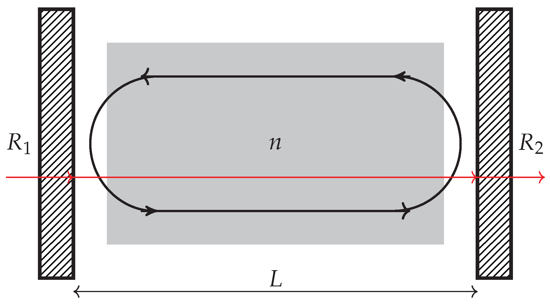
Figure 2.
The angles and the relation between optical indicatrix axes and crystallographic axes.
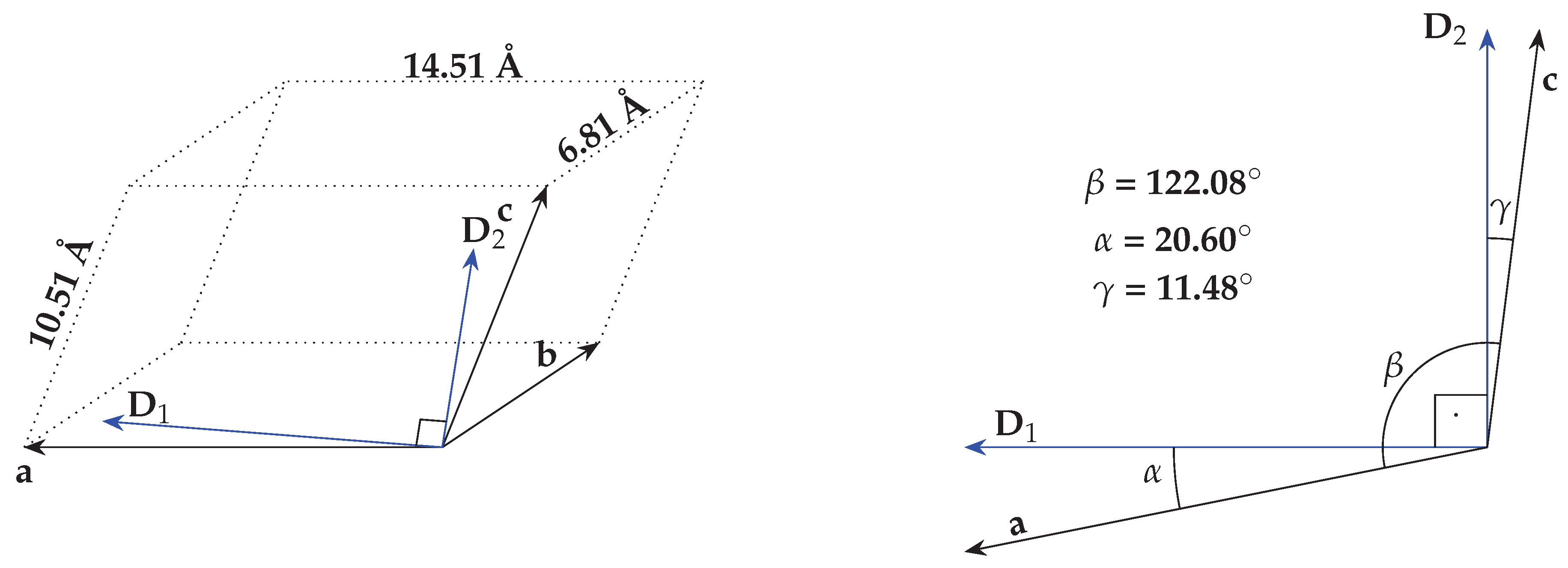
Figure 3.
Schematic view of the crystal geometry employed in FE model.
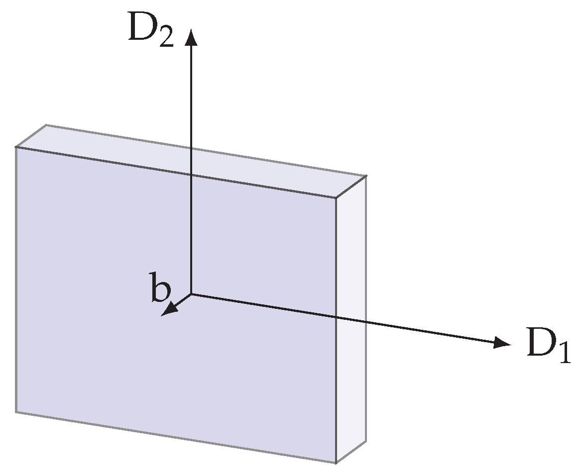
Figure 4.
The measured and calculated values of nin all three directions of pure YSO. The subplots with yellow shading show the same data at lower temperatures. The shading emphasizes the contrast between the measured curves, which have a quadratic shape, and the calculated curve, which has a linear shape.
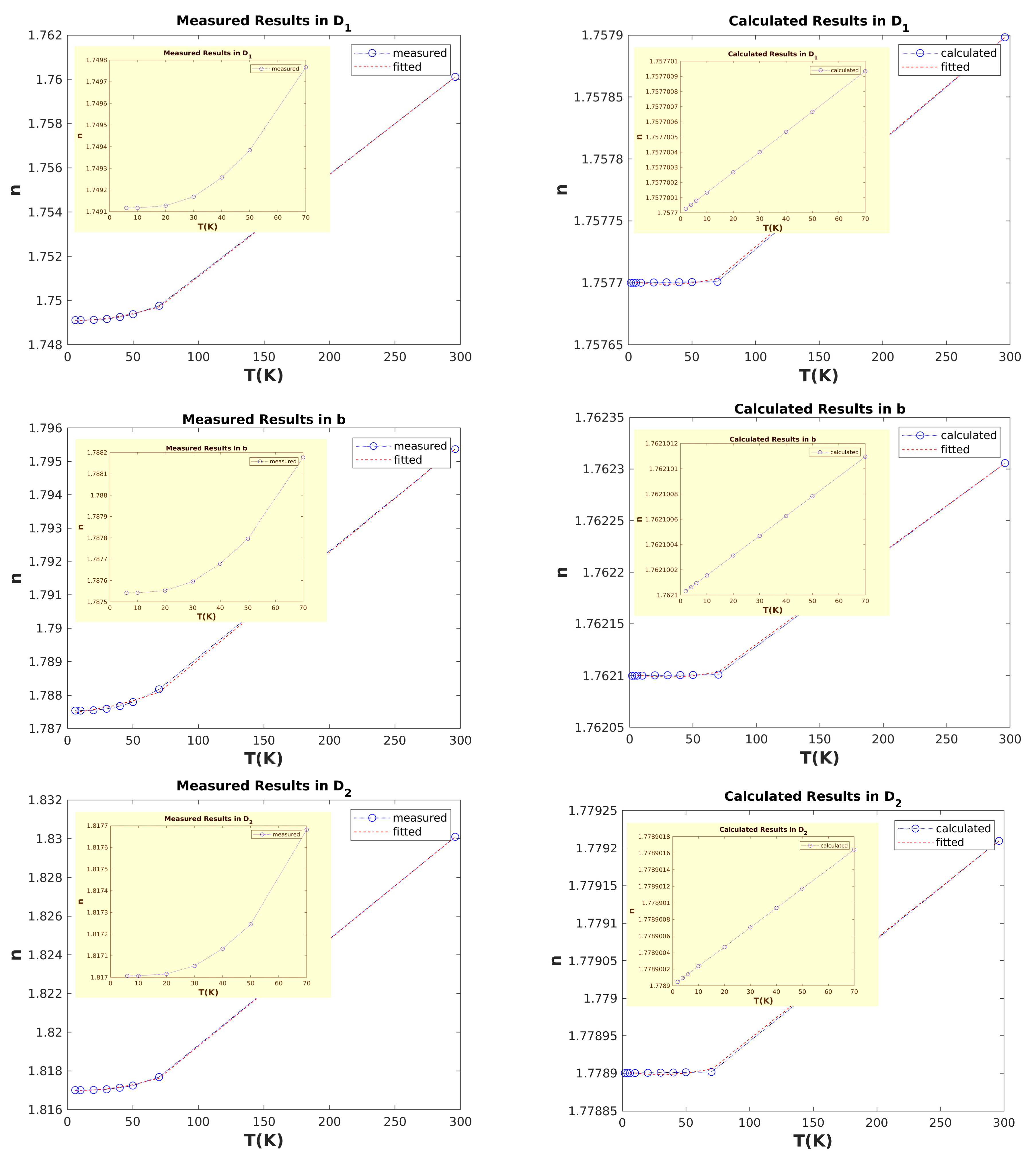
Figure 5.
Refractive indices and frequency shift of pure YSO under load.
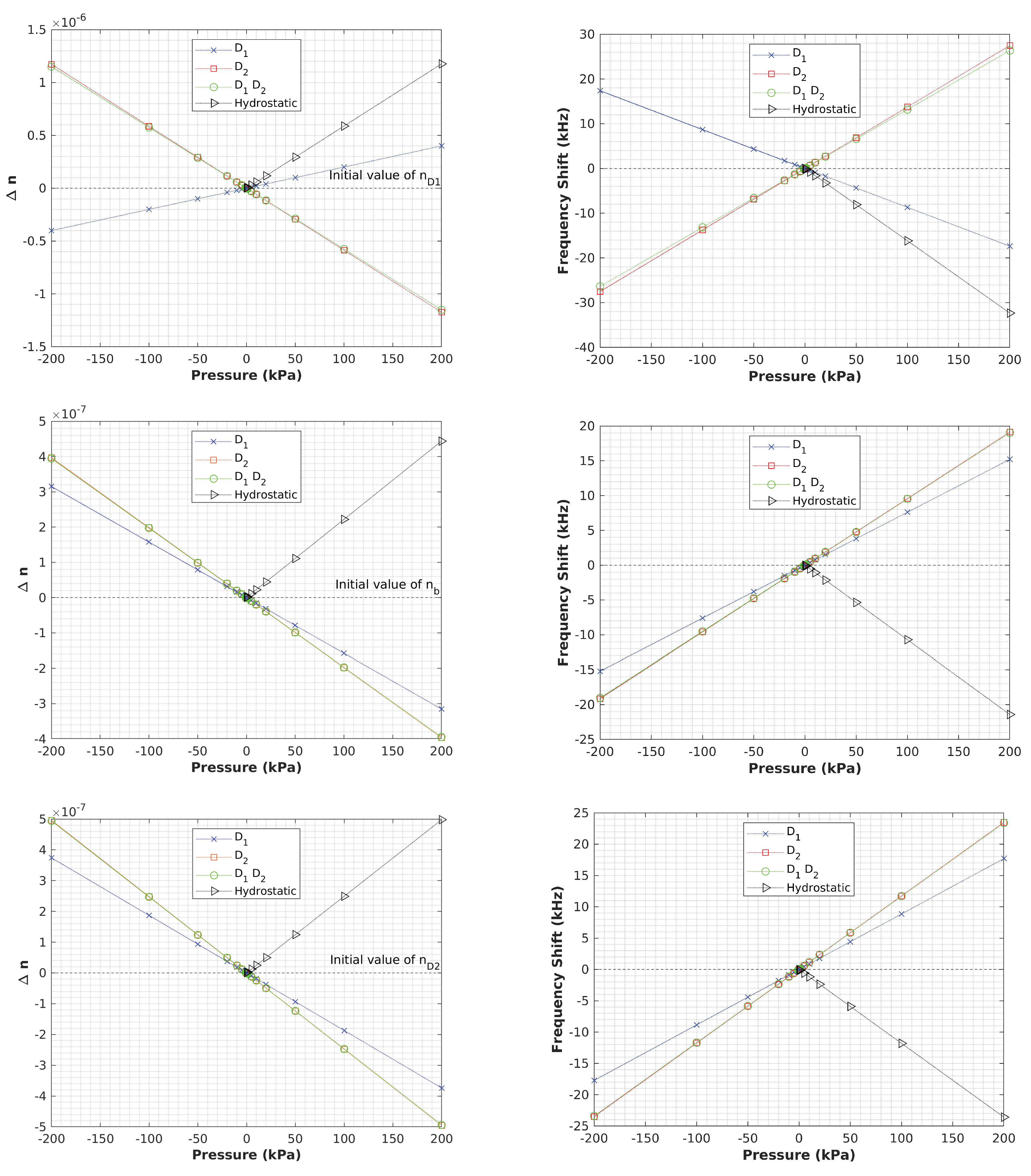
Figure 6.
Refractive indices and frequency shift of Eu-doped YSO under load.
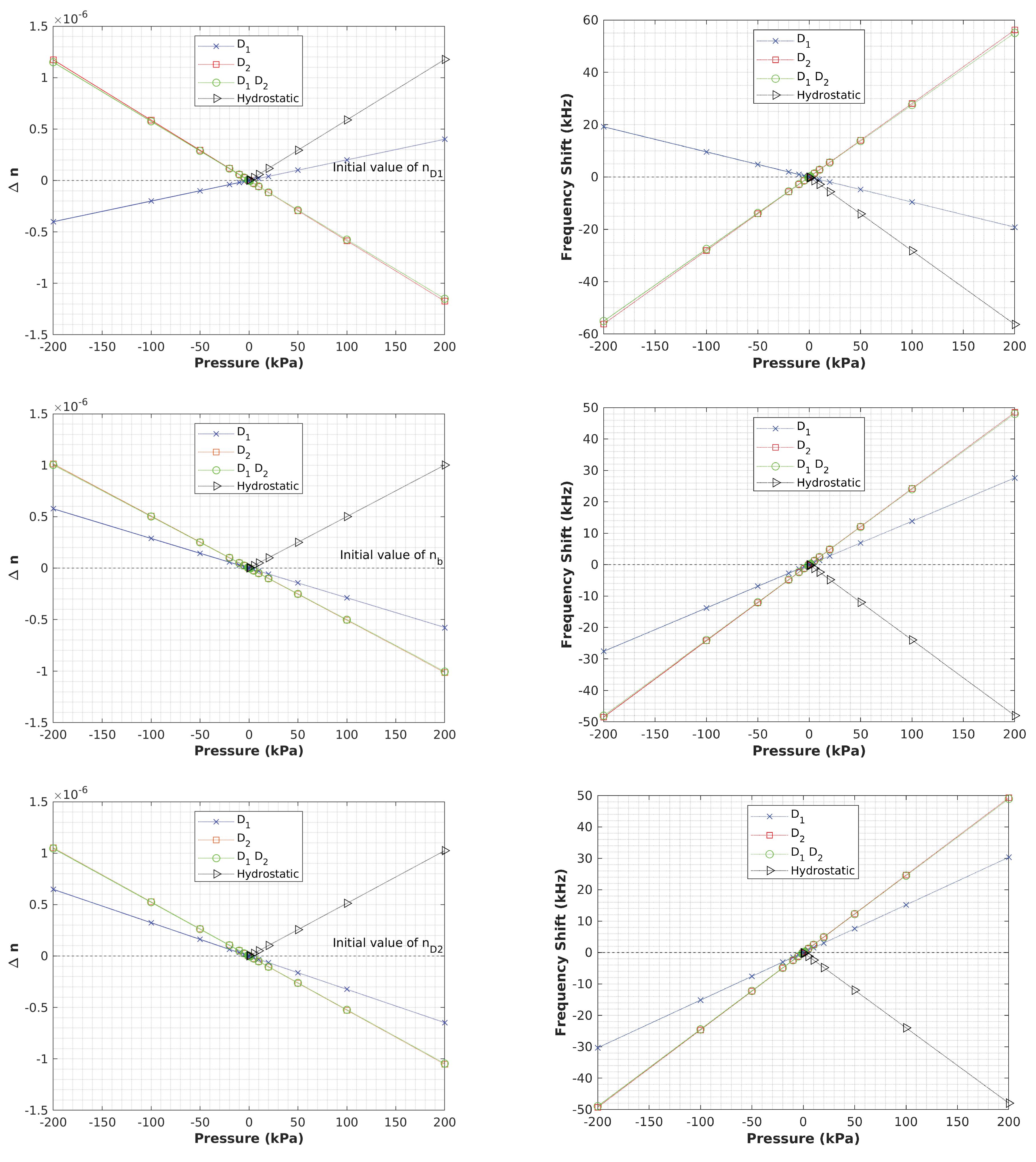

Table 1.
Refractive indices for principal axes of pure YSO and Eu-doped YSO: this work:*. Note: the exp. values are obtained at 632.8 nm.
Table 1.
Refractive indices for principal axes of pure YSO and Eu-doped YSO: this work:*. Note: the exp. values are obtained at 632.8 nm.
| source | ≈ | = | ≈ |
|---|---|---|---|
| YSO-Exp. [25] | 1.780 | 1.784 | 1.811 |
| Exp. [28] | 1.769 | 1.770 | 1.789 |
| YSO-PBE* | 1.8569 | 1.8578 | 1.8822 |
| YSO-PBE0-D3* | 1.7577 | 1.7621 | 1.7789 |
| Eu:YSO-PE0-D3* | 1.7691 | 1.7692 | 1.7892 |
Table 2.
Elastic constants of YSO, and Eu:YSO, in GPa.
| YSO-Exp. [25] | 65.8 | - | - | ±70.6 | 185 | - | - | 83.5 | ±33.0 | 46.5 | ±0.14 | 187 | 65.6 |
| YSO-PBE [9] | 212.21 | 62.78 | 78.65 | 11.64 | 197 | 49.50 | -13.56 | 173.21 | -21.07 | 61.42 | 10.08 | 48.41 | 69.25 |
| YSO-PBE [29] | 226 | 88 | 59 | 5 | 201 | 27 | -0.3 | 156 | -0.2 | 44 | 10 | 67 | 63 |
| Eu:YSO-PBE [9] | 209.35 | 60.17 | 77.59 | 11.47 | 190.82 | 47.39 | -13.62 | 173.15 | -20.99 | 61.21 | 10.03 | 47.70 | 69.24 |
Table 3.
Piezo-optic constants of both pure YSO and Eu:YSO, . Unit=Brewsters, 1B = 10.
| YSO | ||||||||||
|---|---|---|---|---|---|---|---|---|---|---|
| PBE0-D3 | -0.603 | 0.880 | 1.184 | -1.223 | 0.164 | 0.551 | 0.557 | -0.131 | 0.337 | 0.725 |
| Eu:YSO | ||||||||||
| PBE0-D3 | -0.634 | 1.921 | 1.457 | -1.229 | 0.195 | 1.580 | 0.815 | -0.131 | 0.478 | 1.611 |
| YSO | ||||||||||
| PBE0-D3 | 0.313 | 0.365 | -0.353 | -0.037 | -0.504 | -0.073 | 0.459 | -0.594 | 0.117 | -1.476 |
| Eu:YSO | ||||||||||
| PBE0-D3 | 0.440 | 0.489 | 0.032 | -0.268 | -0.442 | -0.281 | 0.269 | -0.572 | 0.025 | -1.526 |
Table 4.
Elasto-optic constants of both pure YSO and Eu:YSO, .
| YSO | ||||||||||
|---|---|---|---|---|---|---|---|---|---|---|
| PBE0-D3 | 0.41 | 0.147 | 0.158 | -0.058 | 0.118 | 0.124 | 0.124 | 0.002 | 0.140 | 0.162 |
| Eu:YSO | ||||||||||
| PBE0-D3 | 0.110 | 0.189 | 0.195 | -0.055 | 0.149 | 0.182 | 0.150 | -0.000 | 0.172 | 0.197 |
| YSO | ||||||||||
| PBE0-D3 | 0.109 | 0.032 | -0.022 | -0.006 | -0.067 | -0.037 | 0.028 | -0.028 | -0.011 | -0.071 |
| Eu:YSO | ||||||||||
| PBE0-D3 | 0.110 | 0.032 | -0.003 | -0.010 | -0.071 | -0.049 | 0.014 | -0.028 | -0.024 | -0.062 |
Table 5.
Comparison of measured and calculated refractive indices versus temperature for pure YSO. The measured data is taken from [10].
Table 5.
Comparison of measured and calculated refractive indices versus temperature for pure YSO. The measured data is taken from [10].
| measured | calculated | Error | |||||||
|---|---|---|---|---|---|---|---|---|---|
| Temp. (K) | n | n | n | n | n | n | Err.D(%) | Err.(%) | Err.D(%) |
| 6 | 1.749(1174) | 1.787(5427) | 1.817(0071) | 1.757(7000) | 1.762(1000) | 1.778(9001) | 0.490 | 1.423 | 2.097 |
| 10 | 1.749(1174) | 1.787(5427) | 1.817(0071) | 1.757(7001) | 1.762(1001) | 1.778(9002) | 0.490 | 1.423 | 2.097 |
| 20 | 1.749(1276) | 1.787(5528) | 1.817(0162) | 1.757(7002) | 1.762(1003) | 1.778(9004) | 0.490 | 1.423 | 2.097 |
| 30 | 1.749(1687) | 1.787(5952) | 1.817(0529) | 1.757(7004) | 1.762(1004) | 1.778(9007) | 0.487 | 1.426 | 2.099 |
| 40 | 1.749(2575) | 1.787(6784) | 1.817(1321) | 1.757(7005) | 1.762(1006) | 1.778(9009) | 0.482 | 1.430 | 2.103 |
| 50 | 1.749(3836) | 1.787(7965) | 1.817(2445) | 1.757(7006) | 1.762(1007) | 1.778(9011) | 0.475 | 1.437 | 2.109 |
| 70 | 1.749(7664) | 1.788(1770) | 1.817(6818) | 1.757(7009) | 1.762(1010) | 1.778(9016) | 0.453 | 1.458 | 2.133 |
| 296 | 1.760(1088) | 1.795(3696) | 1.830(0966) | 1.757(8983) | 1.762(3055) | 1.779(2097) | 0.125 | 1.841 | 2.780 |
| 100 | 1.7(5035) | 1.7(8859) | 1.8(1836) | 1.7(5770) | 1.7(6210) | 1.7(7890) | 0.419 | 1.481 | 2.169 |
| 500 | 1.7(8046) | 1.8(0887) | 1.8(5505) | 1.7(5832) | 1.7(6274) | 1.7(7986) | 1.243 | 2.550 | 4.052 |
| 1000 | 1.8(7438) | 1.8(6975) | 1.9(7115) | 1.7(5933) | 1.7(6366) | 1.7(8127) | 6.083 | 5.610 | 9.543 |
Table 6.
Calculated refractive indices for Eu-doped YSO with respect to temperature.
| Temp. (K) | n | n | n |
|---|---|---|---|
| 2 | 1.769(1000) | 1.769(2000) | 1.789(2000) |
| 4 | 1.769(1001) | 1.769(2001) | 1.789(2001) |
| 6 | 1.769(1001) | 1.769(2002) | 1.789(2002) |
| 10 | 1.769(1003) | 1.769(2003) | 1.789(2004) |
| 20 | 1.769(1006) | 1.769(2007) | 1.789(2009) |
| 30 | 1.769(1009) | 1.769(2011) | 1.789(2014) |
| 40 | 1.769(1013) | 1.769(2015) | 1.789(2018) |
| 50 | 1.769(1016) | 1.769(2019) | 1.789(2023) |
| 70 | 1.769(1023) | 1.769(2027) | 1.789(2032) |
| 100 | 1.769(1032) | 1.769(2038) | 1.789(2045) |
| 296 | 1.769(5465) | 1.769(7177) | 1.789(8166) |
Table 7.
The rate of change of resonance frequency (df/dP) for pure & Eu-doped YSO with respect to the applied load.
Table 7.
The rate of change of resonance frequency (df/dP) for pure & Eu-doped YSO with respect to the applied load.
| LoadAxis | Doped | n | n | n |
|---|---|---|---|---|
| D | no | -0.0869 | 0.0761 | 0.0886 |
| D | yes | -0.0960 | 0.1381 | 0.1517 |
| D | no | 0.1375 | 0.0957 | 0.1174 |
| D | yes | 0.2810 | 0.2424 | 0.2465 |
| DD | no | 0.1318 | 0.0952 | 0.1169 |
| DD | yes | 0.2754 | 0.2402 | 0.2448 |
| Hydrost. | no | -0.1616 | -0.1071 | -0.1179 |
| Hydrost. | yes | -0.2818 | -0.2399 | -0.2399 |
Disclaimer/Publisher’s Note: The statements, opinions and data contained in all publications are solely those of the individual author(s) and contributor(s) and not of MDPI and/or the editor(s). MDPI and/or the editor(s) disclaim responsibility for any injury to people or property resulting from any ideas, methods, instructions or products referred to in the content. |
© 2024 by the authors. Licensee MDPI, Basel, Switzerland. This article is an open access article distributed under the terms and conditions of the Creative Commons Attribution (CC BY) license (http://creativecommons.org/licenses/by/4.0/).
Copyright: This open access article is published under a Creative Commons CC BY 4.0 license, which permit the free download, distribution, and reuse, provided that the author and preprint are cited in any reuse.


