1. Introduction
Society’s reliance on Lithium-ion (Li-ion) batteries is going to increase with the increased focus on electrification of the transportation sector, and shift to more volatile renewable energy sources. However, Li-ion batteries degrade over time, decreasing their available capacity and increasing their resistance; leading to decreasing acceleration and range in electric vehicles (EVs). Thus, determining a battery’s level of degradation, called its state-of-health (SOH), is important to both the safe operation and maintenance of the battery, or the application in which the battery is operated.
Methods used to estimate the SOH of Li-ion batteries fall into one of three categories, physics-driven models, data-driven models, and hybrid models combining aspects of data-driven and physics-driven methods. The physics-driven methods aim to model the internal states and processes of the battery using physics, chemistry, and electrical circuits [
1,
2,
3,
4,
5,
6,
7]. While they can be very accurate when tailored to a specific battery, they tend to be very computationally complicated and inaccurate if applied to different batteries. This is partly the reason for the rise in the use of data-driven methods. Of these methods, the most common include multiple linear regression (MLR) [
8], support vector regression (SVR) [
9,
10,
11,
12], Gaussian process regression (GPR) [
13,
14,
15,
16,
17,
18,
19], and neural networks (NN) [
20,
21,
22,
23,
24]. It has been shown that if enough data is available, then these methods can be used to predict the SOH with very small errors. The main disadvantage of these methods is that they require lots of data, and that most are very complex or essentially black-box methods. This has led to the development of hybrid methods combining data- and physics-driven methods [
25,
26,
27,
28]. These are usually divided into two types; the first use data-driven methods to parameterise physics-driven methods, while the second uses physics to constrain the data-driven methods [
26]. Both approaches are relatively new in the field of SOH estimation, but have been applied to great effect in other areas of research.
Historically, data-driven SOH estimation models have been built using data created in extensive laboratory experiments. This data has typically been created by isolating a single stress-factor at a time, and observing its effect on the degradation of the battery. Furthermore, the charge/discharge pattern has tended to be continuous charging and discharging. However, it has been shown that the degradation of the battery is heavily influenced by its operation (and the order of this operation). Thus, it follows, that for models to achieve good performance in actual operation, when the data is created using continuous charge/discharge, the number of conditions (or combinations of conditions) needs to be exhaustive. This is not only time and resource demanding, but is also limited to the particular type of battery examined (i.e. the materials used to construct it, the manufacturer making it, and the version/generation for this manufacturer). Therefore, the field has, in recent years, started moving from building models based on batteries subjected to these very simple continuous charge/discharge patterns, to batteries aged using more domain-specific operation profiles [
29,
30]. These profiles tend to be more dynamic and a better representation of the degradation behaviour in the specific context, but are also harder to manage as they are more complex and tend to be sparser (in that there will be fewer complete charges or discharges).
With that said, in the case of the dynamic operation profiles in EVs, information about the battery charge capacity, can be extracted every time the vehicle is charged, as the current is relatively consistent. Nevertheless, these charges are not complete, as the vehicle will never be entirely depleted – this would leave the operator of the vehicle stranded – resulting in only partial charges. Previous work on battery SOH estimation using partial charges has shown that information extracted from these can be used to predict the complete capacity of the battery with errors below 1%. However, these methods tend to rely on either extracting information from sub-sequences of the complete charge curve [
31,
32], which cannot be access in operation, extracting information from many partial charges [
33], which makes the model either reliant on the number of partial charges needed to make predictions, or domain adaptation [
33,
34,
35,
36], which in a lot of cases requires fine-tuning. Furthermore, building and evaluating methods based on consistent profiles, even if they are dynamic, will lead to overfitting these methods to the data (including the profile) used to train them. Therefore, this work aims to examine the effect of the number of partial charges used to train the SOH estimation models, and if a dependence on the location of a partial charge within a mission profile can be detected.
The remainder of the paper is organised as follows: the experimental data used to train the models is introduced in
Section 2.1. This is followed by a more precise definition of the partial charges and the features extracted from these partial charges are presented in
Section 2.2. After which
Section 2.3 and
Section 2.4 contain a short explanation of the state-of-health estimation model and feature selection used in this paper. The approaches used to study the sensitivity to, and importance of, the partial charges are found in
Section 2.5. The results of the modelling, sensitivity, and importance are presented in
Section 3. Lastly, conclusions are found in
Section 4.
2. Materials and Methods
2.1. Forklifts and Realistic Load Profiles
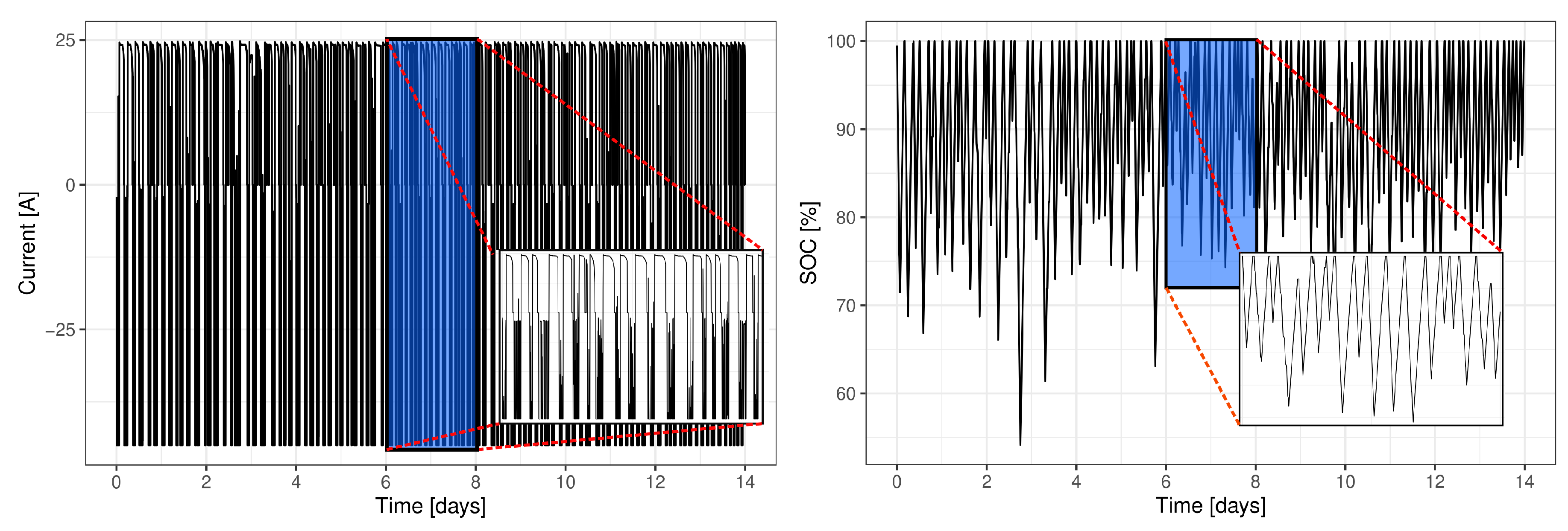
Three Li-ion LFP battery cells were aged using a realistic forklift load profile of approximately two weeks. This profile was distilled from four months of field operation. The current and SOC of the resulting two-week profile is shown in
Figure 1. Furthermore, to accelerate the ageing of the three cells, they were subjected to high temperatures, during operation, of 45, 40, and 35°C, respectively.
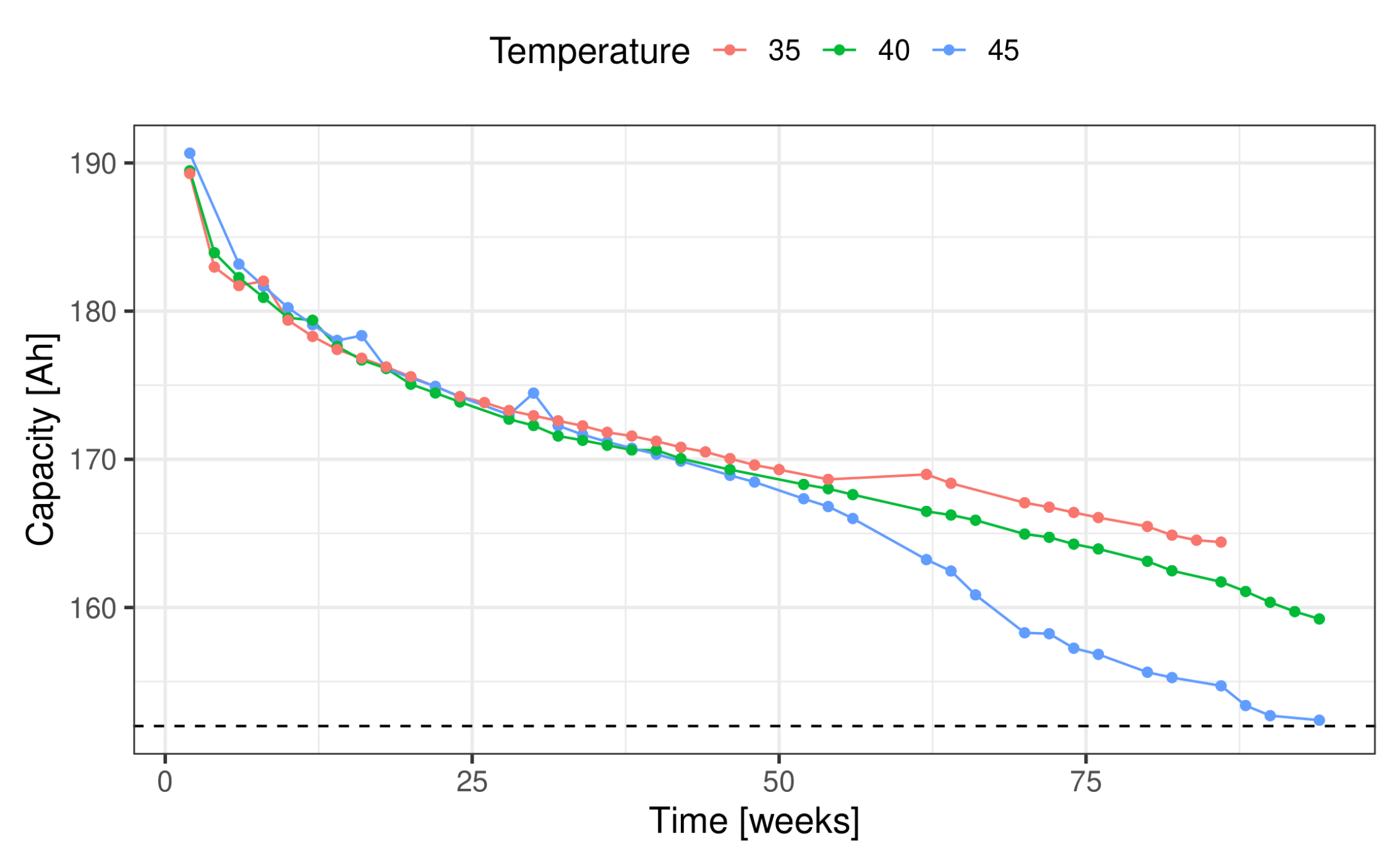
At the end of every round of ageing (i.e. at the end of the two-weeks of operation using the forklift profile), a reference performance test (RPT) is performed (at 25°C) to assess the health of the battery (i.e. the capacity and resistance is measured). This two-step process was repeated until the cell aged at 45°C reached end-of-life (80% of its initial capacity measurement). The resulting capacities obtained for each of the three cells can be seen in
Figure 2. A more thorough introduction and description of the data used can be found in [
37], and the data can be accessed at [
38].
2.2. Partial Charges
In most applications getting an accurate measurement of the capacity is not possible, during operation, as the cell will never be completely discharged (this is also illustrated by the SOC profile found in the right-hand panel of
Figure 1). Thus, between two reference measurements, it is only possible to observe partial charges of the cell. The forklift profile, shown in
Figure 1, contains more than 110 of these partial charges (depending slightly on the criteria used to determine the partial charges).
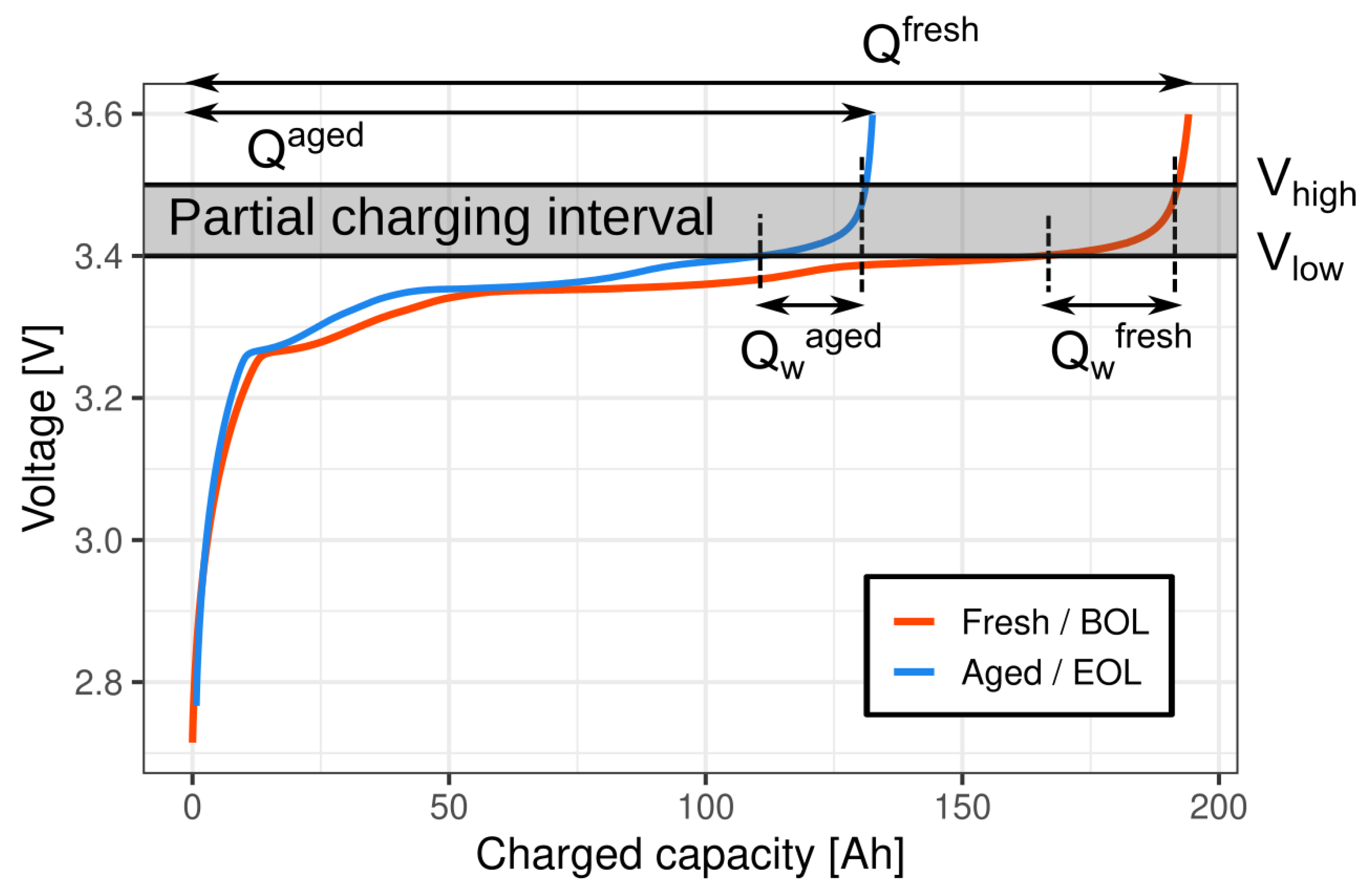
This can be incorporated into the model, given an appropriately chosen voltage interval, it is possible to relate the current accumulated within the interval during charging,
, to the total capacity of the battery,
Q, as show in previous work [
31,
39]. A sketch of the general idea is shown in
Figure 3; given a voltage interval from
to
, the amount of charge within the interval can be related to the total capacity of the cell. This idea has also been extended to other features extracted from the current, voltage, and temperature [
33]. Given a sequence,
, of length
N, the following features are extracted as follows:
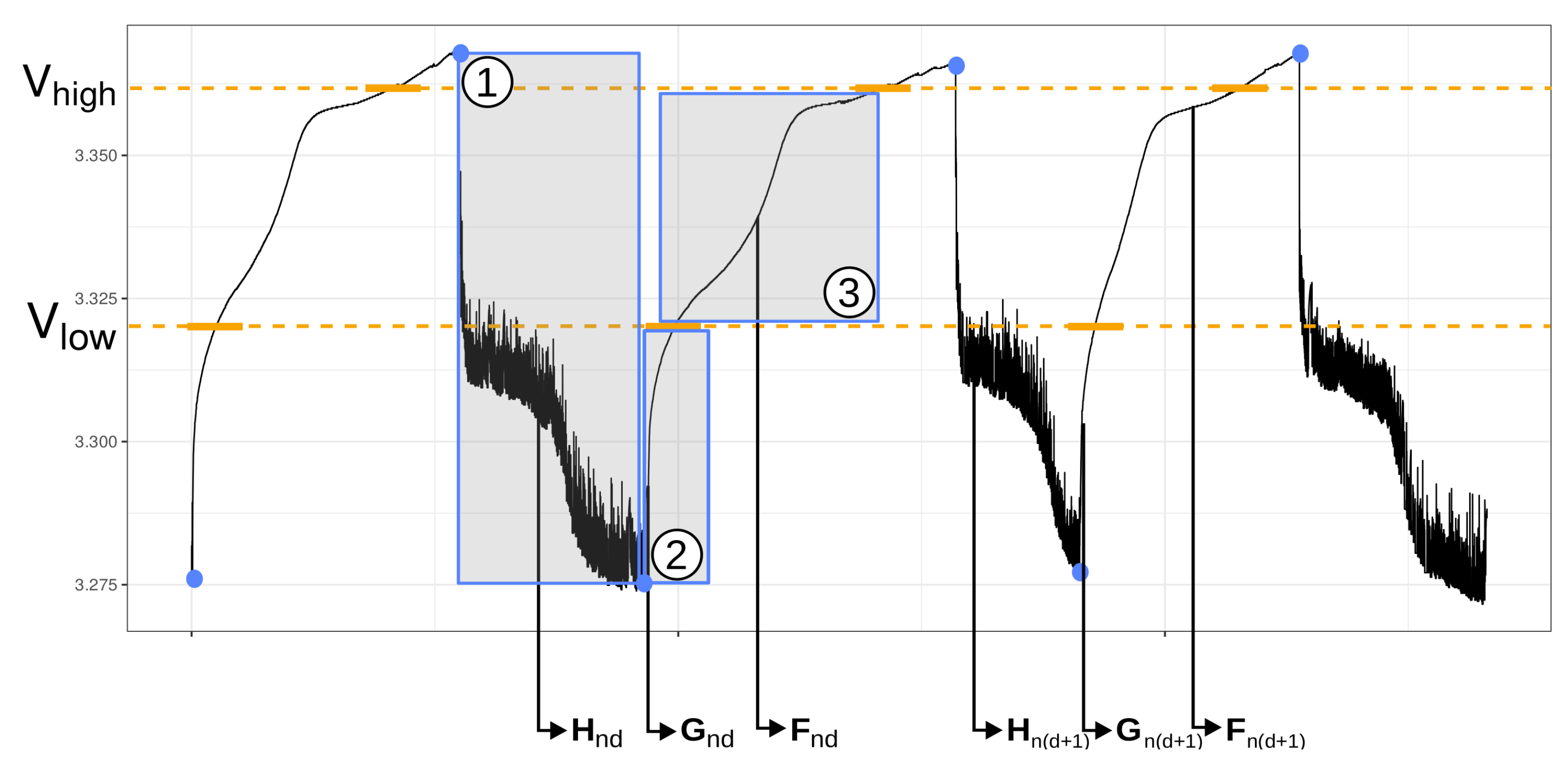
Because the profile contains multiple partial charges, these features can be extracted multiple times between two consecutive RPT capacity measurements, and is used to predict the reference capacity measured at the end of the two-week profile. Furthermore, given a dynamic profile and a predefined voltage interval,
, the profile can be divided into three types of sub-sequence: ➀ the dynamic discharge before a partial charge, ➁ the charge leading up to the beginning of the voltage interval, and ➂ the charge during the voltage interval, as highlighted in
Figure 4. Thus, for the
d’th partial charge in the
n’th round of ageing, it follows that the complete set of features can also be divided into three types, denoted
,
, and
, respectively. However, not all features are extracted from every type of sub-sequence; an overview of what features are extracted for each type of sub-sequence, and from what type of measurement (i.e. current, voltage, temperature, etc.), can be found in
Table 1. These selections are based on expert knowledge, previous work, and consistency of measurement (e.g. temperature is so stable that it is difficult to use higher order moments, like standard deviation, for shorter sequences).
2.3. State-of-Health Modelling
The SOH prediction model used in this paper will be based on multiple linear regression (MLR). MLR maps the features extracted from each partial charge passing through the voltage interval, and the measured capacity at the end of every round of ageing using an affine transformation. MLR was chosen as it is simple, while still having the ability to achieve errors less than 0.5%. Furthermore, the focus is not on the choice of model, but to investigate the sensitivity in both the amount of data, and the dependence on where this data is extracted from, on the performance of the model.
MLR builds a parametric relationship between the capacity,
, and a vector containing all the extracted features,
, as follows:
where
p is the total number of extracted features,
is the intercept,
is the slope corresponding to feature
i,
is the interaction between features
i and
j, and
is a random variable with mean 0 and variance
used to account for noise.
The rounds of ageing are randomly split into two parts, a training-set and validation-set. Using the notation above the complete set of parameters , are then trained, using the training-set, by ordinary least squares (OLS).
2.4. Step-Wise Feature Selection by Leave-One-Out Cross-Validation
In an effort to avoid overfitting, and produce simpler models, leave-one-out cross-validation (LOOCV), on the training-set, will be used to find the combination of features minimising the out-of-sample error. The LOOCV was chosen, as it can be calculated by training the model once using the entire training-set. Given a vector of
N capacity measurements,
, a matrix of corresponding features
X, and a vector of parameters,
, trained using
and
X, then the LOOCV is found as:
where
is a vector containing the features of the
n’th observation and
d’th partial charge, and
is the diagonal entry of the hat matrix, i.e.
, corresponding to
n’th observation and
d’th partial charge.
Step-wise selection, in both directions, using LOOCV as the measure of out-of-sample error, is employed to reduce the number of parameters in the model. That is, parameters, main-effects and interactions (without breaking the hierarchical principle), are allowed to enter, and leave, the model, if it reduces the LOOCV.
2.5. Sensitivity and Importance of Partial Charges
Firstly, in order to investigate the sensitivity in the number of partial charges on the performance of the model, a sequence of limits, , will be successively imposed to restrict the number of partial charges from each round of ageing used to train the model.
Secondly, to explore the importance of each partial charge, more specifically its location within the two-week ageing period, three approaches will be compared when selecting partial charges for training:
- (1)
Using the first L partial charges, i.e. the partial charges closest to the beginning of the round of ageing (and the previous reference measurement).
- (2)
Using the last L partial charges, i.e. the partial charges closest to the end of the round of ageing (and the next reference measurement).
- (3)
Using L partial charges selected at random with replacement, i.e. a partial charge can be used multiple times.
The first two approaches are introduced as reference methods, as these would be the most logical approach when implementing this model in an actual application. That is, the system either only has to store the features extracted from the first
L, or the previous
L, partial charges. The third approach will be used to explore the dependence of the model on particular partial charges. This is possible because the partial charges are chosen at random with replacement, which is equivalent to a type of bootstrapping called
m-out-of-
n bootstrapping [
41]. As a consequence the out-of-bag error (i.e. the error on the observations not used to train the model) can be evaluated. Furthermore, this process is repeated 25 times, giving insight into importance of each partial charge to the model. In each repetition, the root mean square error (RMSE) will be found for each partial charge not used to train the model, the out-of-bag RMSE, and averaged across the 25 repetitions.
3. Results
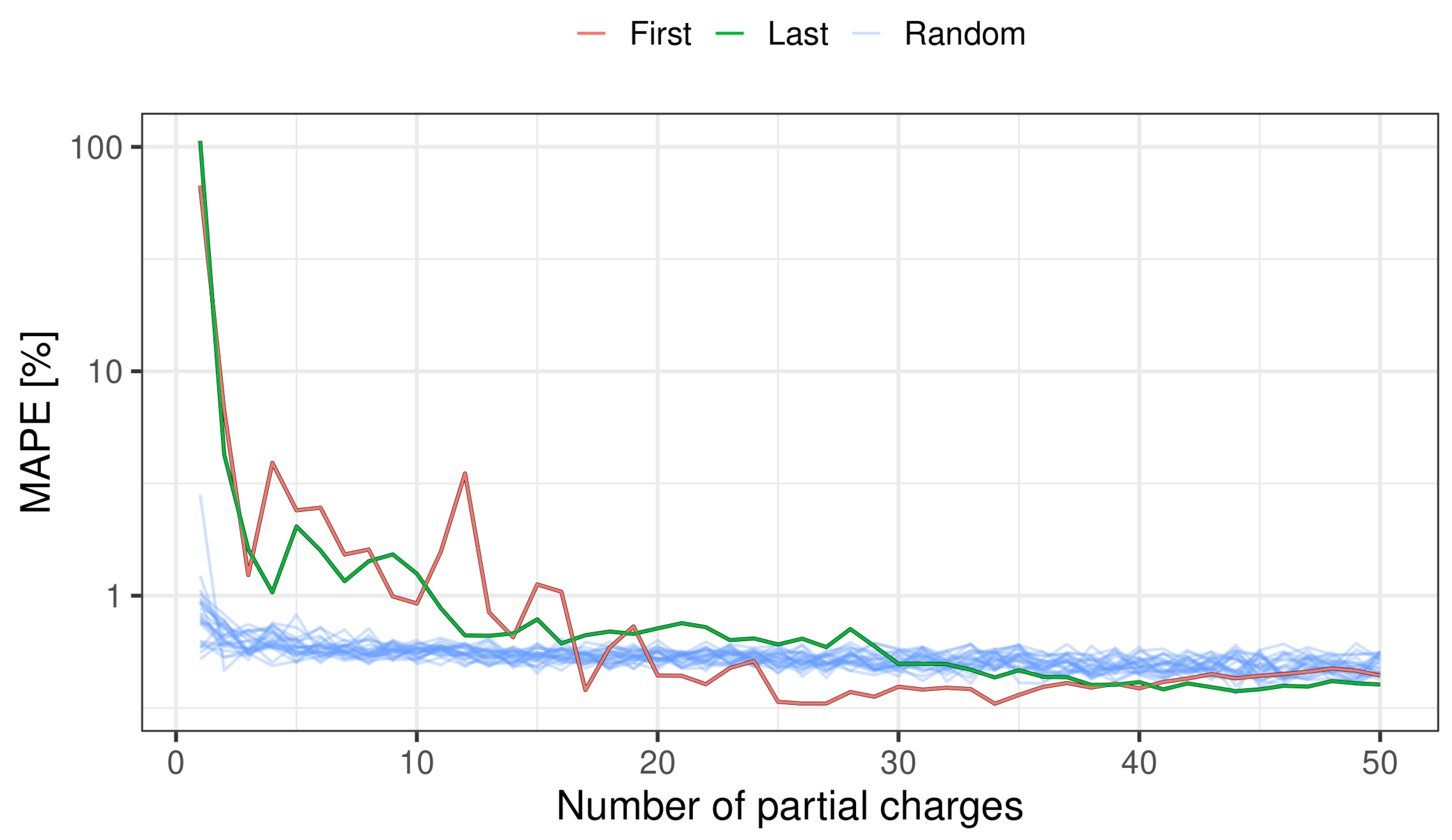
The mean absolute percentage error (MAPE), for all three selection approaches introduced in
Section 2.5, as a function of the number of partial charges used during training of the models is shown in
Figure 5. The results of the models using the first
L partial charges, the last
L partial charges, and the 25 repetitions of
L randomly sampled partial charges, are shown in red, green, and blue, respectively. The figure shows that whether using the first or last
L partial charges makes little difference. However, it takes longer for the error of the first two approaches to to decrease below 1% when compared to using
L random partial charges (for all 25 repetitions). In the former it takes around 10-13, while the latter only requires 2 randomly sampled partial charges. Furthermore, as the number of partial charges increases, the methods selecting the first and last partial charges outperforms the random approach. It is clear that the random sampling approach is quite stable, even when using a very small number of partial charges. Lastly, it is worth noting the three methods should converge as the number of partial charges increases, which is also seen in the figure.
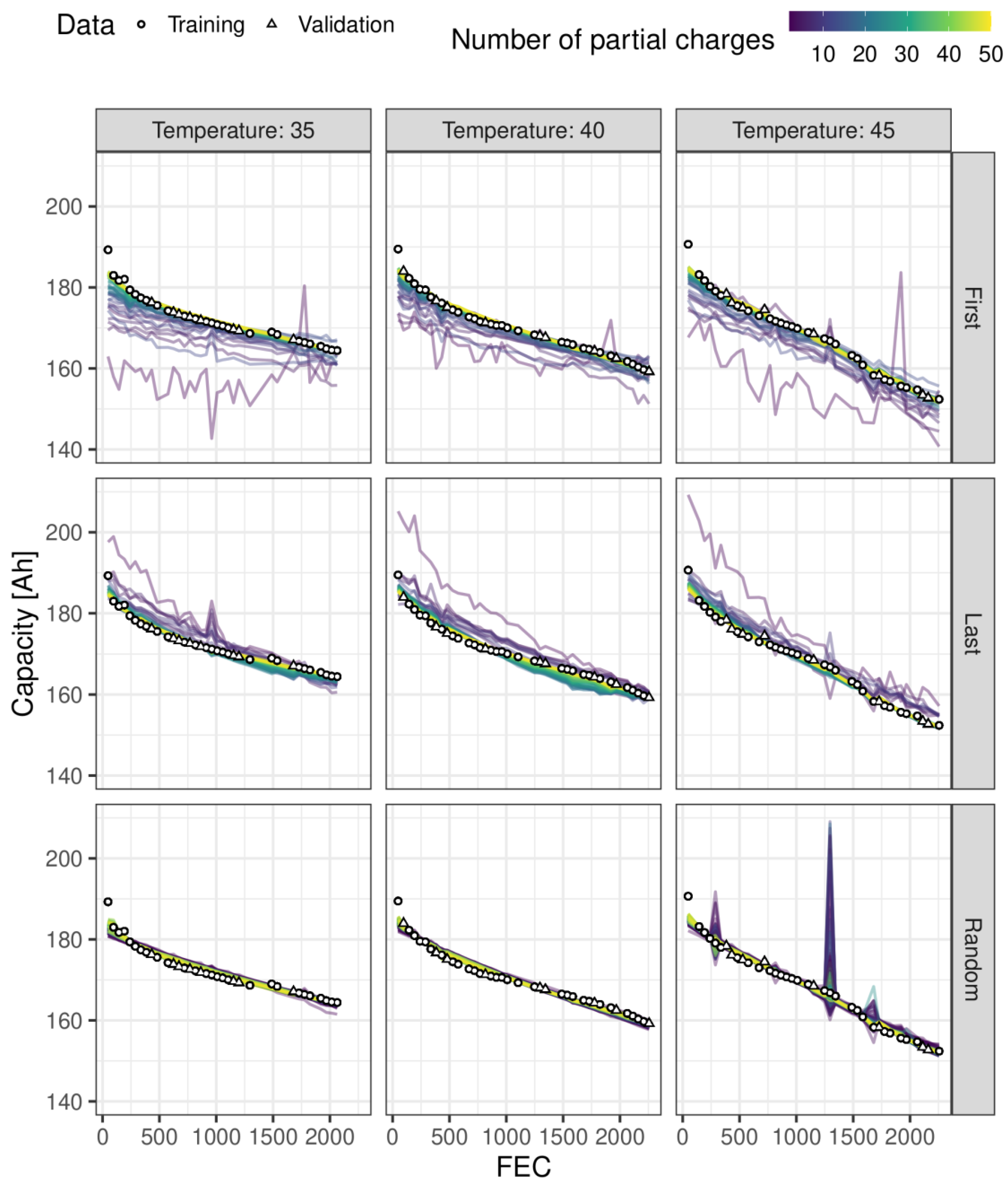
The results of model predictions for each model trained under all three selection approaches of partial charge location is found in the first, second, and third row of
Figure 6, respectively. The figure shows the measured and predicted capacity against the full equivalent cycles (FEC), coloured by the number of partial charges from each round of ageing used to train the models. Furthermore, the measured capacity used for training and validation are shown as circles and triangles, respectively. Focusing on the first two rows, the panels show that as the number of partial charges used to train the models increases, the predicted capacity slowly tends toward the measured capacity. This is completely inline with what should be expected by examining
Figure 5. However, visually comparing the panels of the first and second approach, it looks like the first requires more partial charges than compared to the second approach. This makes intuitive sense, as the last partial charges are going to be closer to the reference measurement the model is trying to predict. The results found in the third row were also mostly in correspondence with what was expected when looking at
Figure 5. The exception being the panel corresponding to 45°C, showing three instances of very large deviations between the predicted and measured capacity for small values of
L. While this is not entirely surprising these deviations are quite large, but decreases as the number of partial charges increases.
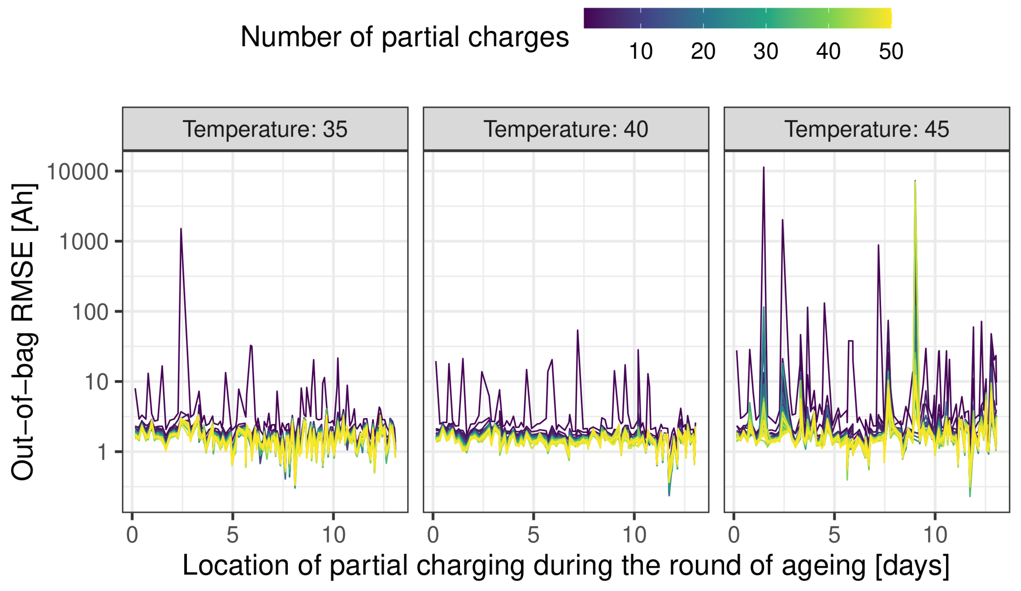
Figure 7 shows the average out-of-bag RMSE, for each partial charges, against the location of the partial charge in the two-week profile to examine its effect on model prediction. The resulting figure should be interpreted as the RMSE, when the partial charge is not used to train the model. When the temperature is 35 and 40°C, the out-of-bag RMSE behaves as is expected, i.e. as the number of partial charges used to train the model increases, the reliance on a particular partial charge decreases, tending to an almost horizontal line as
L increases. However, while the same is mostly true at 45°C, there does seem to be specific partial charges, around the middle and towards the end, which greatly affect the performance of the model. This is in alignment with what was found in
Figure 6, i.e. the large deviations found in
Figure 6 are a direct consequence of these particular partial charges not being included in the training-set (and vice versa).
4. Conclusions
The investigation shows that if only possible to extract, or measure, a few partial charges between two reference measurements, then it is better for these to be sampled at random, rather than those found at either at the beginning or the end of the round of ageing. This result is quite surprising; not just that the validation MAPE is smaller, but also for how long the random approach (for all repetitions!) outperformed the two other approaches. However, as is to be expected, when the number of available partial charges increases, the model build using a more consistent set of partial charges had superior performance. This could indicate that time (or the location of the partial charge within the round of ageing) get implicitly built into the model. While the dependence could be exploited, it is going to be difficult to determine whether this dependence is just an artefact of repeating the profile in every round of ageing. Furthermore, the reason for difference between the non-random and random approaches, is not entirely clear. However, the random sampling approach does seem to benefit in a couple of ways: (1) features extracted from partial charges in close proximity within the two-week profile seem to be more highly correlated, which can lead to instabilities when optimising an MLR, and (2) the partial charges are sampled entirely at random between rounds, i.e. the random sampling approach will create models covering more of the sample space, even with a very small number of partial charges.
Further investigations into the dependence of particular partial charges for models build on the random sampling approach showed, that while there can be some dependence when using a very small number of partial charges, it mostly disappears as the number of partial charges used increased, as was expected. However, while this seems to be accurate for 35 and 40°C, it never seems to disappear entirely at 45°C, which exhibits some dependence on partial charges found at the end the two-week profile. The reason is, again, not entirely clear, but the battery aged at 45°C does degrade at a much higher rate. That is, the difference between the capacity at the beginning and the end of the two-week profile is larger, resulting in a bigger discrepancy between the features extracted at the beginning and end of the profile.
References
- Prasad, G.; Rahn, C. Model based identification of aging parameters in lithium ion batteries. Power Sources 2013, 232, 79–85. [Google Scholar] [CrossRef]
- Zheng, L.; Zhang, L.; Zhu, J.; Wang, G.; Jiang, J. Co-estimation of state-of-charge, capacity and resistance for lithium-ion batteries based on a high-fidelity electrochemical model. Applied Energy 2016, 180, 424–434. [Google Scholar] [CrossRef]
- Andre, D.; Meiler, M.; Steiner, K.; Walz, H.; Soczka-Guth, T.; Sauer, D.U. Characterization of high-power lithium-ion batteries by electrochemical impedance spectroscopy. II: Modelling. Journal of Power Sources 2011, 196, 5349–5356. [Google Scholar] [CrossRef]
- M. Chen.; G. A. Rincon-Mora. Accurate electrical battery model capable of predicting runtime and I-V performance. IEEE Transactions on Energy Conversion 2006, 21, 504–511.
- A. Hentunen.; T. Lehmuspelto.; J. Suomela. Time-Domain Parameter Extraction Method for Thevenin-Equivalent Circuit Battery Models. IEEE Transactions on Energy Conversion 2014, 29, 558–566.
- Stroe, D.I.; Swierczynski, M.; Stroe, A.I.; Knudsen Kær, S. Generalized Characterization Methodology for Performance Modelling of Lithium-Ion Batteries. Batteries 2016, 2. [Google Scholar] [CrossRef]
- Stroe, A.-I.; Knap, V..; Stroe, D.-I. Comparison of lithium-ion battery performance at beginning-of-life and end-of-life. Microelectronics Reliability 2018, 88-90, 1251–1255. [Google Scholar] [CrossRef]
- Vilsen, S.B.; Stroe, D.I. Battery state-of-health modelling by multiple linear regression. Journal of Cleaner Production 2021, 290, 125700. [Google Scholar] [CrossRef]
- Klass, V.; Behm, M.; Lindbergh, G. A support vector machine-based state-of-health estimation method for lithium-ion batteries under electric vehicle operation. Journal of Power Sources 2014, 270, 262–272. [Google Scholar] [CrossRef]
- Patil, M.; Tagade, P.; Hariharan, K.; Kolake, S.; Song, T.; Yeo, T.; Doo, S. A novel multistage Support Vector Machine based approach for Li ion battery remaining useful life estimation. Applied Energy 2015, 159, 285–297. [Google Scholar] [CrossRef]
- Zhao, Q.; Qin, X.; Zhao, H.; Feng, W. State of Charge and State of Health Estimation for Lithium Batteries Using Recurrent Neural Networks. Microelectronics Reliability 2018, 85, 99–108. [Google Scholar] [CrossRef]
- Shu, X.; Li, G.; Shen, J.; Lei, Z.; Chen, Z. A uniform estimation framework for state of health of lithium-ion batteries considering feature extraction and parameters optimization. Energy 2020, 204, 117957. [Google Scholar] [CrossRef]
- Liu, D.; Pang, J.; Zhou, J.; Peng, Y.; Pecht, M. Prognostics for state of health estimation of lithium-ion batteries based on combination Gaussian process functional regression. Microelectronics Reliability 2013, 53, 832–839. [Google Scholar] [CrossRef]
- Richardson, R.; Osborne, M.; Howey, D. Gaussian process regression for forecasting battery state of health. Journal of Power Sources 2017, 357, 209–219. [Google Scholar] [CrossRef]
- Zhou, D.; Yin, H.; Fu, P.; Song, X.; Lu, W.; Yuan, L.; Fu, Z. Prognostics for State of Health of Lithium-Ion Batteries Based on Gaussian Process Regression. Mathematical Problems in Engineering, 2018; pp. 1–1. [Google Scholar]
- Yu, J. State of health prediction of lithium-ion batteries: Multiscale logic regression and Gaussian process regression ensemble. Reliability Engineering and System Safety 2018, 174, 82–95. [Google Scholar] [CrossRef]
- Lyu, Z.; Gao, R. Li-ion battery state of health estimation through Gaussian process regression with Thevenin model. International Journal of Energy Research 2020, 44, 10262–10281. [Google Scholar] [CrossRef]
- Jia, J.; Liang, J.; Shi, Y.; Wen, J.; Pang, X.; Zeng, J. SOH and RUL Prediction of Lithium-Ion Batteries Based on Gaussian Process Regression with Indirect Health Indicators. energies 2020, 13, 1–20. [Google Scholar] [CrossRef]
- Feng, H.; Shi, G. SOH and RUL prediction of Li-ion batteries based on improved Gaussian process regression. Journal of Power Electronics, 2021; 1–1. [Google Scholar]
- Yang, D.; Wang, Y.; Pan, R.; Chen, R.; Chen, Z. A neural network based state-of-health estimation of lithium-ion battery in electric vehicles. 8th International Conference on Applied Energy, Energy Procedia 2017, 105, 2059–2064. [Google Scholar] [CrossRef]
- Kim, J.; Yu, J.; Kim, M.; Kim, K.; Han, S. Estimation of Li-ion State of Health based on Multilayer Perceptron as an EV Application. IFAC-PapersOnLine 2018, 51, 392–397. [Google Scholar] [CrossRef]
- Chaoui, H.; Ibe-Ekeocha, C. State of Charge and State of Health Estimation for Lithium Batteries Using Recurrent Neural Networks. IEEE Trans. Veh. Technol. 2017, 66, 8773–8783. [Google Scholar] [CrossRef]
- You, G.; Park, S.; Oh, D. State of Charge and State of Health Estimation for Lithium Batteries Using Recurrent Neural Networks. IEEE Trans. Ind. Electron. 2017, 64, 4885–4893. [Google Scholar] [CrossRef]
- Wu, Y.; Xue, Q.; Shen, J.; Lei, Z.; Chen, Z.; Liu, Y. State of Health Estimation for Lithium-Ion Batteries Based on Healthy Features and Long Short-Term Memory. IEEE Access 2020, 8, 28533–28547. [Google Scholar] [CrossRef]
- Bian, X.; Wei, Z.; Li, W.; Pou, J.; Sauer, D.U.; Liu, L. State-of-Health Estimation of Lithium-Ion Batteries by Fusing an Open Circuit Voltage Model and Incremental Capacity Analysis. IEEE Transactions on Power Electronics 2022, 37, 2226–2236. [Google Scholar] [CrossRef]
- Guo, W.; Sun, Z.; Vilsen, S.B.; Meng, J.; Stroe, D.I. Review of “grey box” lifetime modeling for lithium-ion battery: Combining physics and data-driven methods. Journal of Energy Storage 2022, 56, 105992. [Google Scholar] [CrossRef]
- Guo, W.; Sun, Z.; Vilsen, S.B.; Blaabjerg, F.; Stroe, D.I. Identification of mechanism consistency for LFP/C batteries during accelerated aging tests based on statistical distributions. e-Prime - Advances in Electrical Engineering, Electronics and Energy 2023, 4, 100142. [Google Scholar] [CrossRef]
- Guo, W.; Li, Y.; Sun, Z.; Vilsen, S.B.; Stroe, D.I. A digital twin to quantitatively understand aging mechanisms coupled effects of NMC battery using dynamic aging profiles. Energy Storage Materials 2023, 63, 102965. [Google Scholar] [CrossRef]
- Li, X.; Yu, D.; Vilsen, S.B.; Store, D.I. Accuracy Comparison of State-of-Health Estimation for Lithium-ion Battery Based on Forklift Aging Profile. 2023 IEEE 14th International Symposium on Power Electronics for Distributed Generation Systems (PEDG), 2023, pp. 584–590. [CrossRef]
- Li, X.; Yu, D.; Vilsen, S.B.; Stroe, D.I. Accuracy comparison and improvement for state of health estimation of lithium-ion battery based on random partial recharges and feature engineering. Journal of Energy Chemistry 2024, 92, 591–604. [Google Scholar] [CrossRef]
- Meng, J.; Cai, L.; Stroe, D.I.; Luo, G.; Sui, X.; Teodorescu, R. Lithium-ion battery state-of-health estimation in electric vehicle using optimized partial charging voltage profiles. Energy 2019, 185, 1054–1062. [Google Scholar] [CrossRef]
- Sui, X.; He, S.; Vilsen, S.B.; Teodorescu, R.; Stroe, D.I. Hyperparameter Optimization in Bagging-Based ELM Algorithm for Lithium-Ion Battery State of Health Estimation. 2023 IEEE Applied Power Electronics Conference and Exposition (APEC), 2023, pp. 1797–1801. [CrossRef]
- Vilsen, S.B.; Stroe, D.I. Transfer Learning for Adapting Battery State-of-Health Estimation From Laboratory to Field Operation. IEEE Access 2022, 10, 26514–26528. [Google Scholar] [CrossRef]
- Tan, Y.; Zhao, G. Transfer Learning With Long Short-Term Memory Network for State-of-Health Prediction of Lithium-Ion Batteries. IEEE Transactions on Industrial Electronics 2020, 67, 8723–8731. [Google Scholar] [CrossRef]
- Kim, S.; Choi, Y.; Kim, K.; Choi, J. Forecasting state-of-health of lithium-ion batteries using variational long short-term memory with transfer learning. Energy Storage 2021, 41, 1–9. [Google Scholar] [CrossRef]
- Che, Y.; Forest, F.; Zheng, Y.; Xu, L.; Teodorescu, R. Health Prediction for Lithium-Ion Batteries Under Unseen Working Conditions. IEEE Transactions on Industrial Electronics, 2024; pp. 1–1. [Google Scholar] [CrossRef]
- Vilsen, S.; Stroe, D. Dataset of lithium-ion battery degradation based on a forklift mission profile for state-of-health estimation and lifetime prediction. Data in Brief 2024, 52, 109861. [Google Scholar] [CrossRef] [PubMed]
- Vilsen, S.; Stroe, D. Lithium-ion battery degradation dataset based on a realistic forklift operation profile. Mendeley Data, V2. 2023. [CrossRef]
- Schaltz, E.; Stroe, D.I.; Nørregaard, K.; Johnsen, B.; Christensen, A. Partial Charging Method for Lithium-Ion Battery State-of-Health Estimation. 2019 Fourteenth International Conference on Ecological Vehicles and Renewable Energies (EVER), 2019, pp. 1–5. [CrossRef]
- Sui, X.; He, S.; Meng, J.; Teodorescu, R.; Stroe, D.I. Fuzzy Entropy-Based State of Health Estimation for Li-Ion Batteries. IEEE Journal of Emerging and Selected Topics in Power Electronics 2021, 9, 5125–5137. [Google Scholar] [CrossRef]
- Alin, A.; Martin, M.; Beyaztas, U.; Pathak, P. Sufficient m-out-of-n (m/n) bootstrap. Journal of Statistical Computation and Simulation 2017, 87, 1742–1753. [Google Scholar] [CrossRef]
Figure 1.
The current and SOC of the two-week forklift profile used to age the Li-ion LFP cells.
Figure 1.
The current and SOC of the two-week forklift profile used to age the Li-ion LFP cells.
Figure 2.
The capacity measured during the RPT performed at the end of every round of ageing, for each of the three cells.
Figure 2.
The capacity measured during the RPT performed at the end of every round of ageing, for each of the three cells.
Figure 3.
A sketch of the partial charging concept. The charge measured within the voltage interval , denoted , changes as the battery ages, and can thus be compared to the total capacity of the cell Q.
Figure 3.
A sketch of the partial charging concept. The charge measured within the voltage interval , denoted , changes as the battery ages, and can thus be compared to the total capacity of the cell Q.
Figure 4.
The three parts of a dynamic load profile of a given voltage interval: ➀ the dynamic discharge before a partial charge, ➁ the charge leading up to the beginning of the voltage interval, and ➂ the charge during the voltage interval.
Figure 4.
The three parts of a dynamic load profile of a given voltage interval: ➀ the dynamic discharge before a partial charge, ➁ the charge leading up to the beginning of the voltage interval, and ➂ the charge during the voltage interval.
Figure 5.
The validation MAPE of the two partial charge selection approaches (using the L last charges and a random selection of charges), against the number of partial charges, from each round ageing, used to train the model.
Figure 5.
The validation MAPE of the two partial charge selection approaches (using the L last charges and a random selection of charges), against the number of partial charges, from each round ageing, used to train the model.
Figure 6.
The capacity against FEC, showing data used for training and validation as circles and triangles, respectively. The predictions of the MLR models, coloured by the number of partial charges, from each round, used to train the models, for both approaches are shown in the first and second row, respectively.
Figure 7.
The RMSE of the out-of-bag observations, against the position of the partial charge in the two-week profile, coloured by the number of partial charges, from each round, to train the model.
Figure 7.
The RMSE of the out-of-bag observations, against the position of the partial charge in the two-week profile, coloured by the number of partial charges, from each round, to train the model.
Table 1.
The features extracted from each of the three types of sub-sequence.
Table 1.
The features extracted from each of the three types of sub-sequence.
|
Disclaimer/Publisher’s Note: The statements, opinions and data contained in all publications are solely those of the individual author(s) and contributor(s) and not of MDPI and/or the editor(s). MDPI and/or the editor(s) disclaim responsibility for any injury to people or property resulting from any ideas, methods, instructions or products referred to in the content. |
© 2024 by the authors. Licensee MDPI, Basel, Switzerland. This article is an open access article distributed under the terms and conditions of the Creative Commons Attribution (CC BY) license (http://creativecommons.org/licenses/by/4.0/).
