Submitted:
28 April 2024
Posted:
29 April 2024
You are already at the latest version
Abstract
In areas like commercial and policy decisions—it's important to know how different treatments affect things and how well they work. However, treatments affect things on average—but now—with fancy computer methods and big sets of data, interest lies in figuring out how treatments might work differently for different people. For instance, let's say instead of just looking at what works for most people, researchers want to know which treatment is best for each person. This would help doctors to decide the right treatment for each patient. This idea isn't just for healthcare—it can help in other areas too, like deciding how to govern employees or making government policies. There are some ways people have been trying to do this already, but they struggle when there are lots of different factors to consider. New computer methods, though, are good at handling lots of factors, but they need a ton of data to work well. Therefore, this study looks at three computer methods that are—Virtual Twin Random Forest (VTRF), Causal Forest (CF), and Causal Net (CN) using real-world data about encouraging people to do manual labour. One problem this study is trying to solve is something called the "winner's curse", where a treatment might seem better than it really is because of how it's predicted by the computer. We are also testing some ideas to see if we can fix this problem and make the predictions more accurate.
Keywords:
Causal Forest
; Causal Net
; Healthcare
; Virtual Twin Random Forest
I. Introduction
Estimating and comprehending causal impacts and treatment—efficacy is necessary for many commercial and policy decisions. In the past, the most common approach has been used to analyze average impacts such as the estimation of Heterogeneous Treatment Effects (HTEs). However, due to the availability of huge datasets—the literature on causal inference, and recent developments in Machine Learning (ML) techniques has gained a lot of attention [1,2,3,4,5]. The topic of whether and which treatment to utilize or allocate optimally is at the heart of the dispute. Consequently, the assignment of an ideal treatment, where each treatment’s efficacy is assessed based on its anticipated treatment effect, is one of the main applications for the detection of HTEs. In recent years—researchers have seen an increase in the popularity of economic literature on causal inference. The focus of HTEs impact estimation and optimal treatment assignment has been the medical sector—in particular—given the increased interest in patient-centered outcomes. However, the potential for cost-effective use cases should not be overlooked in application sectors like the staff management or the efficacy of governmental policies. However, classical nonparametric techniques for estimating HTEs include kernel methods, nearest-neighbor matching, and series estimation. With fewer confounders, these techniques perform well in predictions—but, as the number of covariates increases—performance quickly decreases. This strengthens the case for ML techniques, which frequently require more observations for effective prediction performance yet generally outperform conventional approaches with a wide range of variables. The literature on ML techniques for treatment impact estimation is expanding—raising the questions of which techniques work best for the best treatment assignment and how to compare the techniques using an actual dataset. Therefore, the counterfactual tree-based approach known as Virtual Twin Random Forest (VTRF) [6], the directly estimating tree-based approach known as Causal Forest (CF) [7], and the feed-forward neural network-based approach known as Causal Net (CN) [8] are used in this study. Additionally, we used a method based on [9] to assess the approaches predicting diverse treatment effects for optimal treatment assignment on an empirical dataset about the incentivization of manual work. However, the winner’s curse is a significant obstacle to assigning treatments optimally when adopting diverse treatment. Therefore, we will explain the idea of the winner’s curse, offer shrinkage techniques as a potential remedy, and assess how well the shrinkage techniques work when applied to the ML methods’ predictions on the empirical dataset.
The study is as follows; the background will be seen in the following section. The related works are listed in Section III. The materials and methods are covered in Section IV. The experimental analysis is carried out in Section V, and in Section VI, we provide some conclusions and plans for future research.
II. Background
This section outlined background for estimating Conditional Average Treatment Effects1 (CATE) and HTEs using ML methods such as random forests [10,11,12,13,14,15,16]—are particularly effective for estimating treatment effects because they can capture complex interactions and nonlinearities in the data, which are common when analyzing HTEs. However, CF is advantageous because it leverages the flexibility and scalability of random forests while explicitly focusing on estimating treatment effects. By combining these estimates across multiple trees, CF provides an ensemble estimate of treatment effects. Similarly, CN offers flexibility and scalability in capturing complex relationships between covariates and outcomes, making it suitable for estimating HTEs in high-dimensional data. Generally, it constructs treatment effects by comparing observed outcomes for treated individuals with counterfactual outcomes predicted for untreated individuals. However, unlike traditional neural networks that predict outcomes directly—CN jointly estimates treatment effects and outcomes using a feed-forward neural network with custom layers. This approach allows for the estimation of treatment effects without explicitly observing untreated cases, which is often the case in observational studies. However, HTEs extend this concept further—emphasizing the diverse ways in which treatments affect individuals within a population. By creating synthetic “virtual twins” for untreated individuals, this method enables researchers to approximate the counterfactual scenario where everyone is untreated, facilitating the estimation of treatment effects. This VTRF approach is designed to estimate counterfactual outcomes for untreated individuals. In essence, it quantifies how the effect of a treatment varies depending on individual attributes. Therefore, by leveraging techniques such as regression trees, random forests, VTRF, CF, and CN—researchers can effectively estimate HTEs and make more accurate predictions in observational studies. However, HTE recognizes that one-size-fits-all approaches may not be suitable for interventions, as they may have different impacts on different subgroups. Therefore, ensemble approaches helps to mitigate overfitting and improve generalization performance. By recognizing and accounting for individual differences in response to treatments—researchers can better tailor interventions to specific subgroups and improve overall effectiveness.
III.Related Works
Several studies has been published such as [17] explain the difference between understanding why something happens and just guessing what will happen in policies. [18] suggest a way to pick the best treatment based on what helps people the most. [19] talks about choosing treatments to help society the most—which is different from just making a guess and testing it. Following this, [20] come up with a way to make rules about treatments based on real data. Their study also looked at different ways to figure out how treatments affect different people. [6] used VTRF to guess what would have happened if things were different, and then compares it to what actually happened. [7] see how treatments affect outcomes. [8] used a special kind of math to look at how different factors and treatments affect outcomes together. Similarly, there are other ways to figure out how treatments affect different people such as [21] talk about using a method called Support Vector Machine (SVM) to pick the best treatment for each person. [22] studied an online experiment and used math to predict how treatments affect different people—saying that newer methods like ML work better than older ones in these situations. One main reason to figure out how treatments affect different people is to pick the best treatment for each person such as [9]—whose methods we’ll use to compare models—say that recently people have become more interested in this because of work by [23] on marketing policies. To test our ideas, we’ll use data from an experiment done on Amazon MTurk—a website where people do small tasks for money and where researchers often do experiments. A study by [24] is very similar to ours. They looked at how well a ML could pick the best treatment for people based on their personality. They did two big experiments, and we are using data from the first one. They found that knowing people’s personalities helped predict how well they’d do in the experiment. Using the ML to pick treatments gave better results than just picking the best treatment from the first experiment [25,26,27,28].
IV. Materials and Methods
The empirical analysis that was done is described in this section. We will describe the model’s training and hyperparameter tuning, the dataset, and the method for comparing the best treatment assignment performance in terms of anticipated treatment impacts on an actual data set.
A. Data Analysis
The data used in this study was from [24]—which was conducted in September 2021 over around two and a half weeks with a US-only sample utilizing Amazon MTurk. [24] investigated if, in a follow-up MTurk research, a ML model that assigns individual optimal treatments can perform better than one that assigns merely the best treatment overall. However, we’ll concentrate on the study’s initial phase and the techniques used to contrast the various ML models. Prior to beginning the activity, participants in the study were required to complete a lengthy survey about their social preferences, personality traits, and demographics. In addition to inquiries on age, gender, and educational attainment, the Big 5 personality traits, risk aversion, competitiveness, altruism, positive reciprocity, risk preferences, and loss aversion were also included. Therefore, in the next working job, players might earn points over the course of 10 minutes by pushing the buttons “a” and “b”. A timer, the contestants’ current scores, and their current bonus were all visible to them. The incentive—or lack thereof—to push the buttons and accrue points was determined by the random assignment of each participant to one of six treatments or the control group. The mean values for the treated and untreated observations were 1898 and 1533, respectively. The scores were distributed substantially higher for all treatments than for the control group (see Table 1: Wilcoxon Rank Sum test for α < 1%). Figure 1 shows the average and median results. Interestingly, Wilcoxon Rank Sum tests at the 5% level show that the distribution of average outcomes of treatments one, two, four, and five is distributed significantly above the points of treatments three and six (see Table 1). Figure 2 shows the estimated probability density distributions of the points for the corresponding treatments. Since the reward in treatments three and control was constant regardless of the participant’s point total, there is a density spike at 0. The significant difference between the mean and median can also be explained by this surge. A predetermined set of criteria is used to remove participants from the dataset who did not participate in the experiment in an ordered manner.
B. Training and Tuning
The idea here is to find the best settings for models using a grid search method and three-fold cross-validation. This means trying different settings to see which ones work best—and checking how well they do by splitting the data into three parts and testing them on each part. For each method being used, a model for each of the six treatments will be trained. These models will only use data from the control group and the groups that got each treatment. Then, the model will predict how effective each treatment is. The treatment that the model says works the best will be picked. Choosing the right model isn’t easy when predicting treatment effects. There isn’t a simple way to measure how well the model is doing. Therefore, [29] suggest using something called τ-risk to help pick the best model. They did a study and found that using this method usually leads to models that make the fewest mistakes when guessing the treatment effect. τ-risk works like this—it looks at how close the guesses are to the real outcomes and how close the guesses are—to how likely it is for someone to get a treatment. Similarly, a Lasso-estimator and logistic regression will be used to make these guesses, and they will be trained on the data to ensure they’re doing a good job. τ-risk will be used to pick the best model for both the CF and the CN methods. However, picking the best model for the random forests in the VTRF method is simpler. Mean Squared Error (MSE) will also be used when figuring out the outcomes for the two forests that guess what would have happened if someone didn’t get a treatment [30,31,32,33,34,35]. Then, MSE will be used again when looking at the difference between the predicted outcomes. In theory, τ-risk could be used for the random forests too, but it would take too long because so many different settings would have to be tried. Therefore, sticking with MSE—since it’s faster. This careful process helps ensure that the models are set up right and can accurately predict how effective different treatments are. This way, the results of the analysis can be trusted more.
C. Comparison Method
To check how well the methods work on a real dataset—where we can’t see the true treatment effects—a method like one described by [9] will be used. For instance, look at the cases where the model’s suggested treatment matches the treatment that was randomly given. If the average results of these matched cases are much better than the average results of all treated cases, it suggests the models are doing a good job of picking the best treatments. First, the models will be trained using one set of data and then another set will be used to see how well they predict the effects of different treatments. For each case in the second set, pick the treatment that the model says will have the best effect. Some cases will match the randomly given treatment. These are called “matched” cases. By looking at the average outcomes of these matched cases, one can tell how well the models are doing. If the models are good at picking the best treatment—the average outcome of the matched cases will be higher than for models that aren’t as good. If the average outcome of matched cases is better than the average outcome of all treated cases, it means using the model to assign treatments is better than just assigning treatments randomly. And if the average outcome of matched cases is higher than the average outcome for people who got a specific treatment, it means the model is better than just giving everyone that specific treatment. To make sure our results aren’t just due to chance in how the data is split, this process will be repeated 100 times using different splits. Then, look at the average outcomes across all these repeats. Therefore, treatments three and six didn’t perform as well as the others, as mentioned earlier. So, it’s likely that the models will suggest lower effects for these treatments, and they might not get picked as often. That’s why it’ll also be looked at how well the models do when only considering treatments one, two, four, and five, to make sure they’re not just avoiding treatments three and six to look good.
V. Experimental Analysis
The findings of the empirical analysis that was previously described are presented in this section. We will first discuss the outcomes when all six treatments are used, and then we will discuss the outcomes when a subset of therapies—just treatments one, two, four, and five—are used.
A. Full Treatment Set
In this section—the results of the study’s analysis are shared. Table 2 shows the average outcomes of matched observations for all six treatments, and Figure 3 displays how these outcomes vary across the one hundred times we repeated the cross-validation process for the three methods. For all three methods, the average points of matched observations are higher than the average points for all treatments. This suggests that all models would do a better job than random assignment in assigning treatments. Among the models, the CF performs the best with an average outcome of matched observations of 1982, followed by the VTRF with 1959, and the CN with 1921. Only the CF has a matched average outcome higher than the average outcome in treatment four. However, the average outcome of matched observations for treatment four is lower than the actual average points for treatment four for all models, especially for the VTRF and CF. For treatment five, the difference in outcomes between the VTRF and CF models is significant, indicating that these models correctly assign more competitive-oriented participants to the real-time-feedback treatment. The CF performs much better than the other two models in terms of having a higher average outcome of matched observations than the average outcome of treatment four—occurring 81 out of 100 times (compared to 28/100 for VTRF and 5/100 for CN). For the CF alone, the results suggest that assigning treatment using the model is better than just assigning the best-performing treatment. However, the CN performs much worse than the tree-based models according to the introduced metrics. To understand why the VTRF performs worse than the CF, the observations were also matched based on the training set they were trained on (see Table 3). The VTRF had a much higher average points of matched estimations compared to the CF, indicating that it overfits on the training set.
B. Sub Treatment Set
One challenge previously discussed was those treatments three and six had much lower outcomes compared to the other treatments. This could mean that models might seem to work well just because they avoid giving treatments three and six. To address this, the analysis was done again, but only focusing on treatments one, two, four, and five. The results for this subset of treatments are shown in Table 4, and their distributions over the repeats are in Figure 4. Once more, the CF model performed the best, with an average outcome of matched observations of 1980 and achieving above the mean in all 100 repeats (now 1939, considering only the four used treatments). It also performed well compared to treatment four in 75 out of 100 repeats, slightly less than before. The VTRF did better in this analysis compared to when using all treatments. Its average outcome of matched observations over the hundred repeats is 1970, with 52 out of 100 repeats having a higher average outcome than treatment four. However, in 3 out of 100 repeats, the average outcome of matched observations was lower than the average outcome of treatments one, two, four, and five. The performance of the CN remained lower compared to the other two methods, with an average outcome of matched observations of 1945, slightly higher than before, but still below treatment four’s average outcome and just above the mean outcome of the four treatments. Overall, the results for the subset of treatments are quite similar to those for all treatments. This means that using treatments with similar average outcomes doesn’t change the findings much. One notable difference is that the VTRF performed better in this analysis. This suggests that using the VTRF for treatment assignment might be just as good as assigning only treatment four. One possible reason for this is that the VTRF wrongly assigns many observations to treatment six due to overestimation. This is supported by the fact that the VTRF had more matched assignments compared to the CF but with lower average outcomes. Additionally, the average outcomes of matched observations for the VTRF increased for all four treatments in the subset analysis, while they decreased for the CN and the CF.
VI. Conclusions and Future Works
As causal inference becomes more popular, predicting the best treatment using ML methods is becoming important in many areas. When comparing three methods—VTRF, CN, and CF—on real data, the CF seems to be the best at assigning the best treatment. It shows that picking the treatment with the highest predicted effect from the CF leads to better outcomes than just picking the best overall treatment. The VTRF and the CN are better than random assignment but not as good as the CF. In a smaller set of treatments, the VTRF seems to do as well as just picking treatment four. Even though the VTRF doesn’t perform as well overall, it shouldn’t be dismissed. It’s easier to understand and use than the CF, especially for people who aren’t familiar with causal inference. However, one reason the VTRF might not perform as well overall is that it tends to overfit. This means it gets too good at predicting outcomes based on the data it was trained on, so it doesn’t do as well on new data. The CN didn’t perform as well as the other methods. There could be a few reasons for this. The number of observations might have been too low for the neural networks to work well. Also, tuning neural networks is harder than tuning tree-based methods like the CF. The methods used to tune the CN might not have been the best for the data. Plus, the hyperparameter grids used might not have been the best fit. But expanding the grids would have taken too long to compute for this study.
VII. Declarations
Funding
No funds, grants, or other support was received.
Conflict of Interest
The authors declare that they have no known competing for financial interests or personal relationships that could have appeared to influence the work reported in this paper.
Data Availability
Data will be made on reasonable request.
Code Availability
Code will be made on reasonable request.
References
- V. Kanaparthi, “Exploring the Impact of Blockchain, AI, and ML on Financial Accounting Efficiency and Transformation,” Jan. 2024, Accessed: Feb. 04, 2024. [Online]. Available: https://arxiv.org/abs/2401.15715v1.
- V. Kanaparthi, “Robustness Evaluation of LSTM-based Deep Learning Models for Bitcoin Price Prediction in the Presence of Random Disturbances,” Jan. 2024. [CrossRef]
- V. Kanaparthi, “Examining Natural Language Processing Techniques in the Education and Healthcare Fields,” International Journal of Engineering and Advanced Technology, vol. 12, no. 2, pp. 8–18, Dec. 2022. [CrossRef]
- V. Kanaparthi, “Credit Risk Prediction using Ensemble Machine Learning Algorithms,” in 6th International Conference on Inventive Computation Technologies, ICICT 2023 - Proceedings, 2023, pp. 41–47. [CrossRef]
- V. Kanaparthi, “AI-based Personalization and Trust in Digital Finance,” Jan. 2024, Accessed: Feb. 04, 2024. [Online]. Available: https://arxiv.org/abs/2401.15700v1.
- J. C. Foster, J. M. G. Taylor, and S. J. Ruberg, “Subgroup identification from randomized clinical trial data,” Statistics in Medicine, vol. 30, no. 24, pp. 2867–2880, Oct. 2011. [CrossRef]
- S. Wager and S. Athey, “Estimation and Inference of Heterogeneous Treatment Effects using Random Forests,” Journal of the American Statistical Association, vol. 113, no. 523, pp. 1228–1242, Jul. 2018. [CrossRef]
- M. H. Farrell, T. Liang, and S. Misra, “Deep Neural Networks for Estimation and Inference,” Econometrica, vol. 89, no. 1, pp. 181–213, Jan. 2021. [CrossRef]
- Gg. J. Hitsch and S. Misra, “Heterogeneous Treatment Effects and Optimal Targeting Policy Evaluation,” SSRN Electronic Journal, Nov. 2018. [CrossRef]
- P. Kaur, G. S. Kashyap, A. Kumar, M. T. Nafis, S. Kumar, and V. Shokeen, “From Text to Transformation: A Comprehensive Review of Large Language Models’ Versatility,” Feb. 2024, Accessed: Mar. 21, 2024. [Online]. Available: https://arxiv.org/abs/2402.16142v1.
- G. S. Kashyap, K. Malik, S. Wazir, and R. Khan, “Using Machine Learning to Quantify the Multimedia Risk Due to Fuzzing,” Multimedia Tools and Applications, vol. 81, no. 25, pp. 36685–36698, Oct. 2022. [CrossRef]
- N. Marwah, V. K. Singh, G. S. Kashyap, and S. Wazir, “An analysis of the robustness of UAV agriculture field coverage using multi-agent reinforcement learning,” International Journal of Information Technology (Singapore), vol. 15, no. 4, pp. 2317–2327, May 2023. [CrossRef]
- G. S. Kashyap et al., “Revolutionizing Agriculture: A Comprehensive Review of Artificial Intelligence Techniques in Farming,” Feb. 2024. [CrossRef]
- M. Kanojia, P. Kamani, G. S. Kashyap, S. Naz, S. Wazir, and A. Chauhan, “Alternative Agriculture Land-Use Transformation Pathways by Partial-Equilibrium Agricultural Sector Model: A Mathematical Approach,” Aug. 2023, Accessed: Sep. 16, 2023. [Online]. Available: https://arxiv.org/abs/2308.11632v1.
- S. Naz and G. S. Kashyap, “Enhancing the predictive capability of a mathematical model for pseudomonas aeruginosa through artificial neural networks,” International Journal of Information Technology 2024, pp. 1–10, Feb. 2024. [CrossRef]
- G. S. Kashyap, A. E. I. Brownlee, O. C. Phukan, K. Malik, and S. Wazir, “Roulette-Wheel Selection-Based PSO Algorithm for Solving the Vehicle Routing Problem with Time Windows,” Jun. 2023, Accessed: Jul. 04, 2023. [Online]. Available: https://arxiv.org/abs/2306.02308v1.
- J. Kleinberg, J. Ludwig, S. Mullainathan, and Z. Obermeyer, “Prediction policy problems,” in American Economic Review, May 2015, vol. 105, no. 5, pp. 491–495. [CrossRef]
- T. Kitagawa and A. Tetenov, “Who Should Be Treated? Empirical Welfare Maximization Methods for Treatment Choice,” Econometrica, vol. 86, no. 2, pp. 591–616, Mar. 2018. [CrossRef]
- C. F. Manski, “Statistical treatment rules for heterogeneous populations,” Econometrica, vol. 72, no. 4, pp. 1221–1246, Jul. 2004. [CrossRef]
- K. Hirano and J. R. Porter, “Asymptotics for Statistical Treatment Rules,” Econometrica, vol. 77, no. 5, pp. 1683–1701, Sep. 2009. [CrossRef]
- K. Imai and M. Ratkovic, “Estimating treatment effect heterogeneity in randomized program evaluation,” Annals of Applied Statistics, vol. 7, no. 1, pp. 443–470, Mar. 2013. [CrossRef]
- M. Taddy, M. Gardner, L. Chen, and D. Draper, “A Nonparametric Bayesian Analysis of Heterogenous Treatment Effects in Digital Experimentation,” Journal of Business and Economic Statistics, vol. 34, no. 4, pp. 661–672, Oct. 2016. [CrossRef]
- D. Simester, A. Timoshenko, and S. I. Zoumpoulis, “Efficiently evaluating targeting policies: Improving on champion vs. Challenger experiments,” Management Science, vol. 66, no. 8, pp. 3412–3424, Jan. 2020. [CrossRef]
- S. Opitz, D. Sliwka, T. Vogelsang, and T. Zimmermann, “The Targeted Assignment of Incentive Schemes,” SSRN Electronic Journal, Oct. 2022. [CrossRef]
- V. K. Kanaparthi, “Navigating Uncertainty: Enhancing Markowitz Asset Allocation Strategies through Out-of-Sample Analysis,” Dec. 2023. [CrossRef]
- V. Kanaparthi, “Transformational application of Artificial Intelligence and Machine learning in Financial Technologies and Financial services: A bibliometric review,” Jan. 2024. [CrossRef]
- V. K. Kanaparthi, “Examining the Plausible Applications of Artificial Intelligence & Machine Learning in Accounts Payable Improvement,” FinTech, vol. 2, no. 3, pp. 461–474, Jul. 2023. [CrossRef]
- V. Kanaparthi, “Evaluating Financial Risk in the Transition from EONIA to ESTER: A TimeGAN Approach with Enhanced VaR Estimations,” Jan. 2024. [CrossRef]
- A. Schuler, M. Baiocchi, R. Tibshirani, and N. Shah, “A comparison of methods for model selection when estimating individual treatment effects,” Apr. 2018, Accessed: Apr. 28, 2024. [Online]. Available: https://arxiv.org/abs/1804.05146v2.
- G. S. Kashyap et al., “Detection of a facemask in real-time using deep learning methods: Prevention of Covid 19,” Jan. 2024, Accessed: Feb. 04, 2024. [Online]. Available: https://arxiv.org/abs/2401.15675v1.
- G. S. Kashyap, A. Siddiqui, R. Siddiqui, K. Malik, S. Wazir, and A. E. I. Brownlee, “Prediction of Suicidal Risk Using Machine Learning Models.” Dec. 25, 2021. Accessed: Feb. 04, 2024. [Online]. Available: https://papers.ssrn.com/abstract=4709789.
- S. Wazir, G. S. Kashyap, K. Malik, and A. E. I. Brownlee, “Predicting the Infection Level of COVID-19 Virus Using Normal Distribution-Based Approximation Model and PSO,” Springer, Cham, 2023, pp. 75–91. [CrossRef]
- H. Habib, G. S. Kashyap, N. Tabassum, and T. Nafis, “Stock Price Prediction Using Artificial Intelligence Based on LSTM– Deep Learning Model,” in Artificial Intelligence & Blockchain in Cyber Physical Systems: Technologies & Applications, CRC Press, 2023, pp. 93–99. [CrossRef]
- G. S. Kashyap, D. Mahajan, O. C. Phukan, A. Kumar, A. E. I. Brownlee, and J. Gao, “From Simulations to Reality: Enhancing Multi-Robot Exploration for Urban Search and Rescue,” Nov. 2023, Accessed: Dec. 03, 2023. [Online]. Available: https://arxiv.org/abs/2311.16958v1.
- S. Wazir, G. S. Kashyap, and P. Saxena, “MLOps: A Review,” Aug. 2023, Accessed: Sep. 16, 2023. [Online]. Available: https://arxiv.org/abs/2308.10908v1.
Figure 1.
The mean and median results for each treatment are shown in these graphs.

Figure 2.
The estimated kernel density functions for the points for each treatment are shown in this figure.
Figure 2.
The estimated kernel density functions for the points for each treatment are shown in this figure.
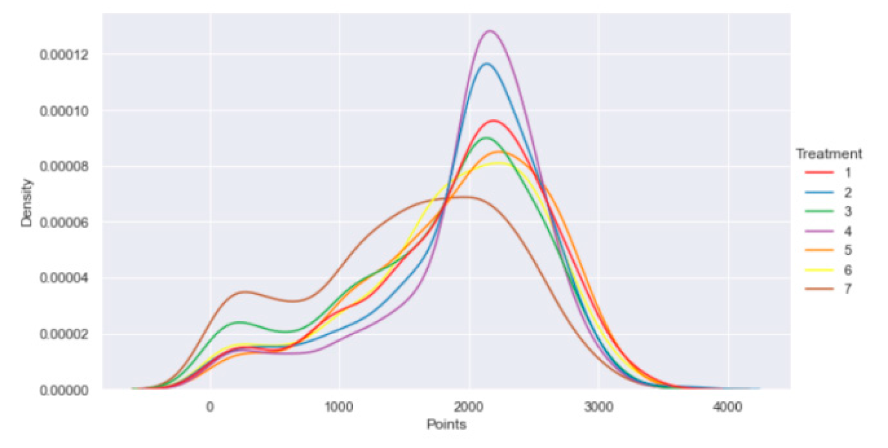
Figure 3.
The distribution of the average result of matched observations for each of the 100 separate three-fold cross-validation repetitions for full treatment..
Figure 3.
The distribution of the average result of matched observations for each of the 100 separate three-fold cross-validation repetitions for full treatment..
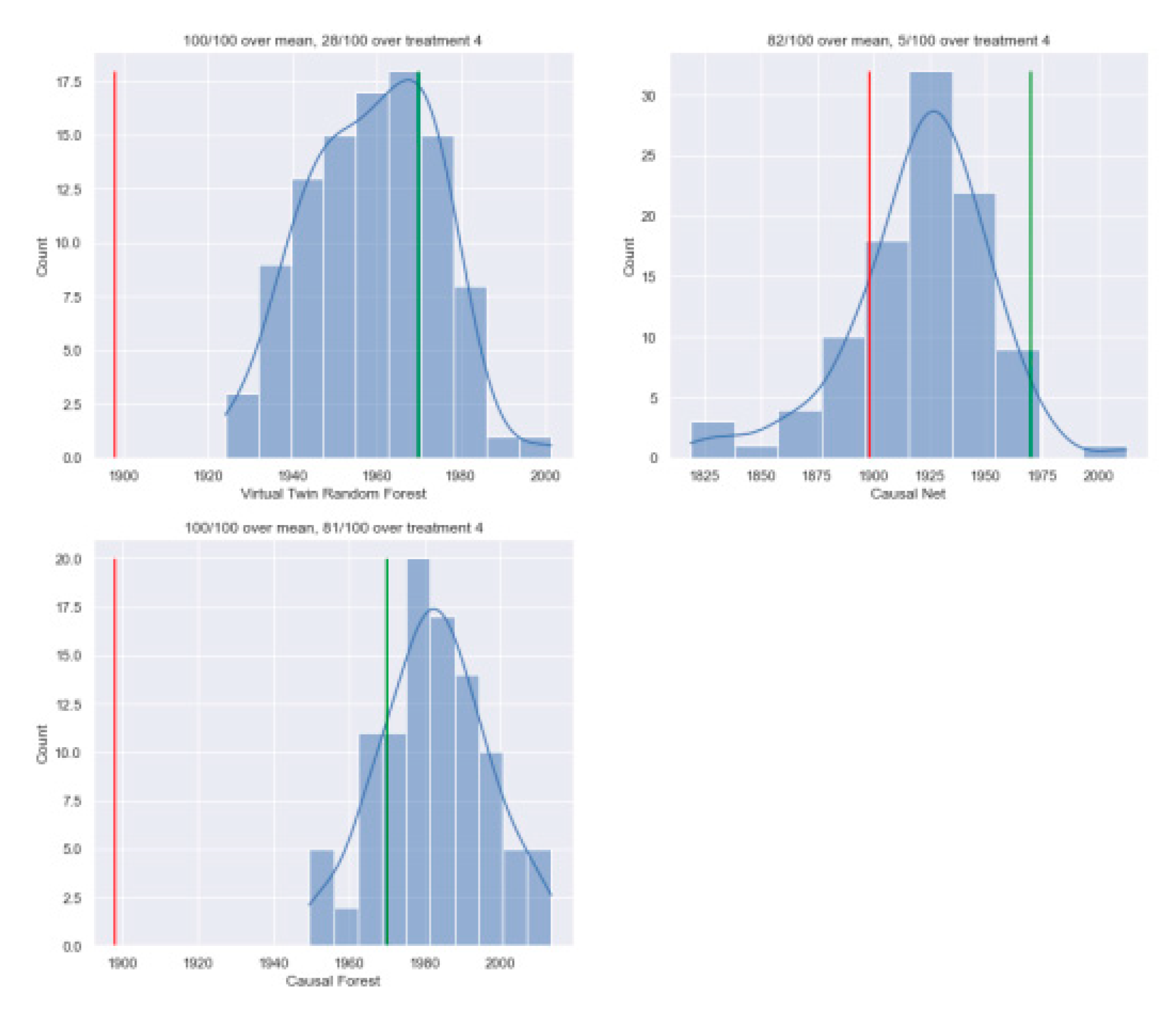
Figure 4.
The distribution of the average result of matched observations for each of the 100 separate three-fold cross-validation repetitions for subset treatment.
Figure 4.
The distribution of the average result of matched observations for each of the 100 separate three-fold cross-validation repetitions for subset treatment.
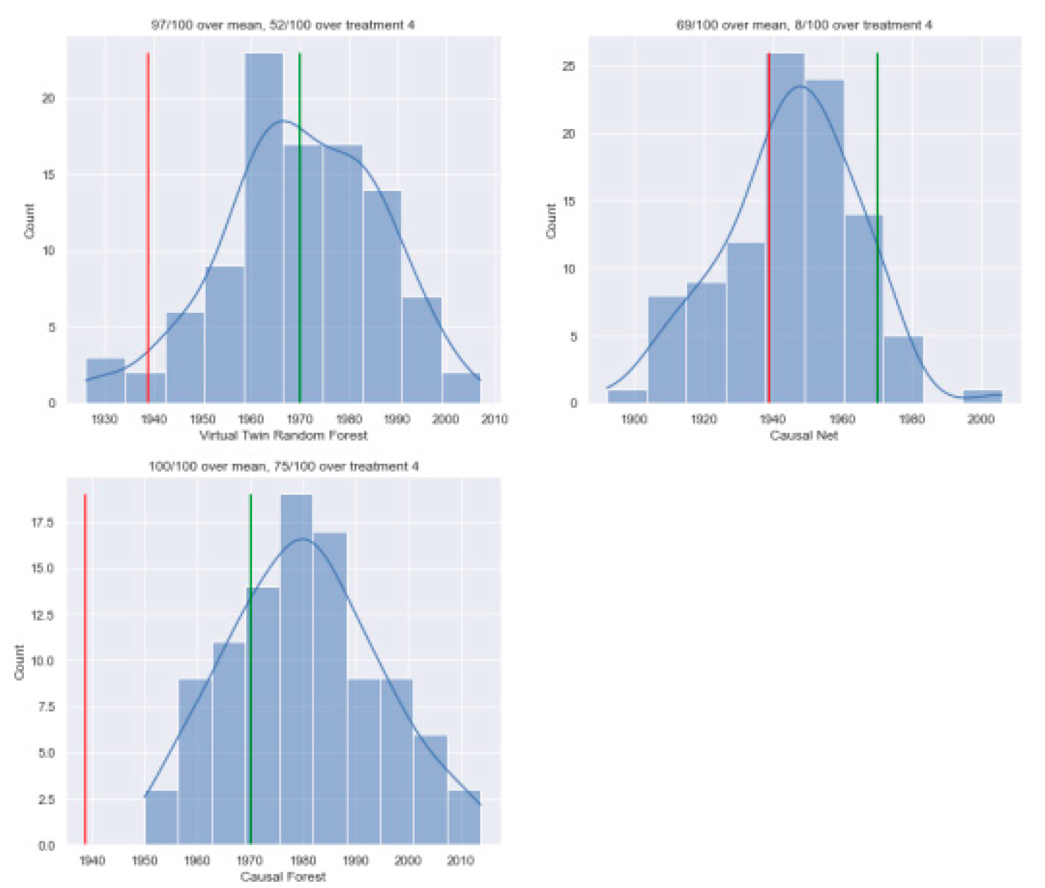

Table 1.
The p-values for the wilcoxon rank sum tests are displayed in this table. x and y represent the sample points, respectively, where the treatment and row value are comparable, and where the treatment and column value, respectively, are treated. the control group is the seventh treatment.
Table 1.
The p-values for the wilcoxon rank sum tests are displayed in this table. x and y represent the sample points, respectively, where the treatment and row value are comparable, and where the treatment and column value, respectively, are treated. the control group is the seventh treatment.
| X/Y | T1 | T2 | T3 | T4 | T5 | T6 | T7 |
|---|---|---|---|---|---|---|---|
| T1 | 0.5 | 0.5544 | 0.0 | 0.9014 | 0.5344 | 0.0468 | 0.0 |
| T2 | 0.4456 | 0.5 | 0.0 | 0.8942 | 0.5024 | 0.0268 | 0.0 |
| T3 | 1.0 | 1.0 | 0.5 | 1.0 | 1.0 | 0.9939 | 0.0 |
| T4 | 0.0986 | 0.1058 | 0.0 | 0.5 | 0.1353 | 0.0009 | 0.0 |
| T5 | 0.4656 | 0.4976 | 0.0 | 0.8647 | 0.5 | 0.0475 | 0.0 |
| T6 | 0.9532 | 0.9732 | 0.0061 | 0.9991 | 0.9525 | 0.5 | 0.0 |
| T7 | 1.0 | 1.0 | 1.0 | 1.0 | 1.0 | 1.0 | 0.5 |
Table 2.
Average of matched observations: not shrunken and full treatment set.
| T1 | T2 | T3 | T4 | T5 | T6 | Overall | |
|---|---|---|---|---|---|---|---|
| VTRF | 1935 | 1925 | 1932 | 1815 | 2135 | 1974 | 1959 |
| (9848) | (12328) | (919) | (27381) | (25300) | (10005) | (85781) | |
| CN | 1938 | 1963 | 1791 | 1957 | 1977 | 1796 | 1921 |
| (10431) | (5927) | (4008) | (23265) | (25338) | (17148) | (86117) | |
| CF | 2136 | 1895 | 2063 | 1788 | 2194 | 2133 | 1982 |
| (7721) | (5950) | (25) | (37917) | (30109) | (2280) | (84002) | |
| Avg. | 1926 | 1930 | 1764 | 1970 | 1931 | 1871 | 1898 |
| (87900) | (86500) | (87500) | (84800) | (87400) | (84500) | (518600) |
Table 3.
JS stands for the James stein shrinker, var for the variance shrinker, and average outcome of matched observations—training set: full treatment set and shrunken. While k shows the shrinkers shrinking toward the average treatment prediction of the specific treatment, indicates the shrinkers shrinking toward the average treatment impact of the entire set of treatments applied.
| Models | T1 | T2 | T3 | T4 | T5 | T6 | Overall |
|---|---|---|---|---|---|---|---|
| VTRF | 2315 | 2325 | 2526 | 2241 | 2302 | 2505 | 2339 |
| (22233) | (30722) | (6296) | (65269) | (52553) | (49024) | (226097) | |
| VTRF (JS ) | 2298 | 2321 | 2534 | 2240 | 2301 | 2507 | 2336 |
| (21828) | (29951) | (5648) | (65754) | (53033) | (48727) | (224941) | |
| VTRF (JS ) | 2301 | 2322 | 2526 | 2240 | 2301 | 2504 | 2337 |
| (21383) | (29688) | (6291) | (65604) | (53134) | (49416) | (225516) | |
| VTRF (Var ) | 2310 | 2318 | 2756 | 2211 | 2301 | 2649 | 2303 |
| (20482) | (30367) | (10) | (80422) | (51408) | (19640) | (202329) | |
| VTRF (Var ) | 2313 | 2328 | 2526 | 2241 | 2304 | 2511 | 2339 |
| (22087) | (30865) | (5892) | (66867) | (51883) | (47470) | (225064) | |
| CN | 1925 | 1929 | 1770 | 1969 | 1931 | 1871 | 1904 |
| (24609) | (59397) | (31939) | (39592) | (5230) | (10829) | (171596) | |
| CN (JS ) | 1924 | 1929 | 1770 | 1969 | 1931 | 1871 | 1905 |
| (24624) | (59953) | (31357) | (39592) | (5230) | (10829) | (171585) | |
| CN (JS ) | 1923 | 1929 | 1769 | 1969 | 1929 | 1871 | 1901 |
| (25826) | (56473) | (34269) | (38414) | (5820) | (10829) | (171631) | |
| CF | 2543 | 2398 | 2576 | 1966 | 2394 | 2608 | 2243 |
| (20206) | (16041) | (101) | (73792) | (61361) | (7023) | (178524) | |
| CF (JS ) | 2532 | 2386 | 2641 | 1956 | 2388 | 2624 | 2222 |
| (18080) | (13636) | (35) | (75905) | (62716) | (4550) | (174922) | |
| CF (JS ) | 2541 | 2389 | 2594 | 1953 | 2373 | 2601 | 2223 |
| (16595) | (12361) | (109) | (73468) | (66663) | (6355) | (175551) | |
| CF (Var ) | 2503 | 2420 | 0 | 1965 | 2441 | 2715 | 2174 |
| (18156) | (11274) | (0) | (99352) | (43650) | (490) | (172922) | |
| CF (Var ) | 2546 | 2402 | 2564 | 1965 | 2398 | 2607 | 2240 |
| (19688) | (15978) | (93) | (75149) | (60381) | (6672) | (177961) | |
| Average | 1926 | 1930 | 1764 | 1970 | 1931 | 1871 | 1898 |
| (175800) | (173000) | (175000) | (169600) | (174800) | (169000) | (1037200) |
Table 4.
The outcomes of the misra-matching threefold cross-validation, performed 100 times, are displayed in this table.
Table 4.
The outcomes of the misra-matching threefold cross-validation, performed 100 times, are displayed in this table.
| Models | T1 | T2 | T4 | T5 | Overall |
|---|---|---|---|---|---|
| VTRF | 1971 | 1954 | 1831 | 2136 | 1970 |
| (12102) | (15824) | (30825) | (27436) | (86187) | |
| CausalNet | 1910 | 1932 | 1948 | 1962 | 1945 |
| (14266) | (9394) | (29754) | (32824) | (86238) | |
| CausalForest | 2145 | 1926 | 1786 | 2185 | 1980 |
| (8606) | (6443) | (38062) | (30855) | (83966) | |
| Average | 1926 | 1930 | 1970 | 1931 | 1939 |
| (87900) | (86500) | (84800) | (87400) | (346600) |
| 1 | CATE refers to the variation in treatment effects across different groups of individuals—often defined by their covariates or characteristics. |
Disclaimer/Publisher’s Note: The statements, opinions and data contained in all publications are solely those of the individual author(s) and contributor(s) and not of MDPI and/or the editor(s). MDPI and/or the editor(s) disclaim responsibility for any injury to people or property resulting from any ideas, methods, instructions or products referred to in the content. |
© 2024 by the authors. Licensee MDPI, Basel, Switzerland. This article is an open access article distributed under the terms and conditions of the Creative Commons Attribution (CC BY) license (http://creativecommons.org/licenses/by/4.0/).
Copyright: This open access article is published under a Creative Commons CC BY 4.0 license, which permit the free download, distribution, and reuse, provided that the author and preprint are cited in any reuse.


