
Submitted:
25 April 2024
Posted:
28 April 2024
You are already at the latest version
Abstract
Total ankle replacement (TAR) implants are an effective option to restore the range of motion of the ankle joint for arthritic patients. An effective tool for analyzing these implants’ mechanical performance and longevity in-silico is finite element analysis (FEA). ABAQUS FEA was used to statically analyze the von Mises stress and contact pressure on the articulating surface of the bearing component in two newly installed fixed-bearing total ankle replacement implants (the Wright Medical INBONE II and the Exactech Vantage). This ultra-high molecular weight polyethylene (UHMWPE) bearing commonly fails and is the cause for surgeon revisions. Six different FEA models for various gait percentages during stance (10%-60%) were created. They varied in magnitude of the compressive load and the ankle dorsiflexion/plantarflexion angle. The results indicated that the von Mises stress and contact pressure distributions increased as compressive load increased, and the largest magnitudes occurred at high dorsiflexion angles (15-30°). High magnitudes occurred in regions where the thickness of the bearing was the least. Additionally, high contact pressures were examined in areas near the talar component's edge or at the bearing's edges. To the author’s knowledge, this is the first study available to the research community that analyzes the Vantage implant with FEA. This study lays an essential foundation for future researchers in presenting a thorough literature review of TAR and methods for a simple FEA model setup. This study provides valuable information that can be beneficial to medical company designers and orthopedic surgeons in understanding the stress response and contact pressure of TAR implants during use.
Keywords:
bioengineering
; total ankle replacement (TAR)
; bearing component
; UHMWPE
; finite element analysis
; von Mises stress
; contact pressure
; ABAQUS
1. Introduction
The ankle, or tibiotalar joint, is a hinged synovial articulation between the distal tibia, talus, and fibula bones. The lateral malleolus of the distal fibula forms the outer border of the joint, while the medial malleolus of the distal tibia forms the inner border of the joint. The distal tibia, or tibial plafond, forms the superior border, and the talar dome trochlear surface forms the inferior border. All surfaces of the joint are lined by articular cartilage, a viscoelastic connective tissue that facilitates load transmission [1,2]. The bony articulations are further stabilized by strong collateral ligaments medially and laterally. A schematic of an ankle joint is shown Figure 1.
The ankle joint has six degrees of freedom. The greatest motion occurs in the sagittal plane, functioning to provide dorsiflexion and plantarflexion. Dorsiflexion refers to the motion when the foot moves upwards towards the tibia, whereas plantarflexion refers to the foot moving downwards towards the ground. Normal, non – arthritic ankles have approximately 50-75° total range of motion (ROM) in the sagittal plane, on average 10-20° dorsiflexion and 40-55° plantarflexion [3,34,35]. Ankle planes of motion are shown in Figure 2.
Gait refers to the pattern of walking. One gait cycle is the time between heel strike to heel strike of a limb. The stance phase of gait, which makes up 60% of the gait cycle, is the time during which the foot is in contact with the ground. This phase is of primary significance when analyzing stress on the ankle joint. The swing phase is the period of time when the foot is not in direct contact with the ground, and comprises the remainder of the gait cycle.
The stance phase is subdivided into initial contact and loading response, mid-stance, terminal stance, and pre-swing, as shown in Figure 3.
Data from Martinelli [5] of normal ankle dorsiflexion and plantarflexion angles are plotted in Figure 4. During the first 10% of gait, initial contact and loading response, the heel contacts the ground, the foot everts and the ankle dorsiflexors eccentrically contract. During the subsequent mid stance, 10-30% of the stance phase, the tibia externally rotates, and plantarflexors eccentrically contract. At terminal stance and pre-swing, 30-60% of the stance phase, the plantarflexors concentrically contract, and the foot internally rotates [6].
Ankle joint osteoarthritis is a debilitating degenerative disorder resulting in loss of articular cartilage, functionally limiting pain and loss of motion [7]. Surgical treatment to address end stage ankle arthritis includes ankle fusion or total ankle arthroplasty (TAA) [8].
TAA has several advantages over ankle arthrodesis, including preservation of ankle ROM, more normal gait mechanics, and minimizing adjacent joint stress [5]. Surgical technique involves resection of the degraded tibial plafond and talar dome articular and subchondral bone surfaces and replacing them with the corresponding TAA components. Figure 5 shows a labeled diagram of a TAA implant.
TAA results in significant improvement in patient-reported outcome measures including decreased pain, improved mobility, physical and mental function, and quality of life [16,17,36]
The tibial and talar components typically have porous coated pegs and stems that insert into native bone for primary fixation and bony ingrowth. Bone cement can be used to augment fixation if needed. [9,10]. These components are typically made of Cobalt Chromium Molybdenum (CoCrMo), a high stiffness and high strength material.
The bicondylar bearing component is made of Ultra High Molecular Weight Polyethylene (UHMWPE). This material has low wear rate, chemical inertness, biocompatibility, high crystallinity, high ductility, and material toughness. Typically, it is cross-linked and injected with Vitamin E as an antioxidant to eliminate free radicals, decrease wear rate and promote longevity [11,12].
The primary failure modes of TAA are polyethylene wear and aseptic loosening [18]. The locations of these failure modes are labeled in Figure 6. Aseptic loosening is a non-infectious failure of prosthetic component fixation, leading to unstable and unintended motion of the component [37].
Polyethylene wear occurs from abnormal stress concentration leading to particulate formation that can function as debris within the joint. This leads to activation of specialized cells called macrophages, that leads to bone destruction, or osteolysis, around the implant components. [4,13]. Further micromotion at the bone and implant interface leads to gross loosening, which eventually lead to painful implant subsidence [14]. The von Mises stress is an equivalent stress that is an important characteristic in determining whether a material yields under maximum loading.
Long term TAA implant survivorship is greater than 90% at 10 years [13]. However, the longer-term results of fourth generation implants at 15-20 years are still limited [15], highlighting the need for in-silico testing of these TAA implants.
The primary aim of this study was to investigate the mechanical behavior of two commonly used TAA fixed-bearing implants, the Wright Medical INBONE II and the Exactech Vantage, under axial loading and varying ankle position during the stance phase of the gait cycle. Static structural analysis was performed to highlight the implant areas most susceptible to failure based on identified points of maximum loading. Von Mises stress response and contact pressure distribution on the bearing component was further sub-characterized during all four components of the stance phase.
2. Methods
The process towards developing the FEA model in ABAQUS is outlined in Figure 9. The implant geometry was created in SolidWorks 2023 and the FEA was performed in ABAQUS 6.25.
2.1. Implant Geometry Development
Obtaining precise geometry of the implants was not possible due to the proprietary nature of their designs. Wright Medical and Exactech provided limited dimensions of the implant components within their surgical technique guides including length, width, and height of each of the components. Therefore a reverse-engineering process was utilized to model the implants. A size 2 implant was chosen, supported by the prior study by Yu [23] in their FEA study of the INBONE II. This is the smallest size available, and is appropriate for a conservative estimate on implant stresses given that the highest stresses are expected from the smallest size. The coronal and sagittal views of the INBONE II tibial component with the corresponding implant dimensions per size are shown in Figure 10a. The proportions of the component elements were assumed to be true to the real implant, and screen clips were taken from these images and optimized using Microsoft Paint. Then, these views were saved as DXFs to import into SolidWorks (Figure 10b). This maintains the feature-to-feature relationships since the proportions were assumed to be true. The features were exported to create the completed part in Figure 10c.
The exact dimensions of the INBONE II tibial and talar component stems and pegs were not disclosed by the manufacturer, and only the thickness of the bearing was pro-vided for the Vantage. Data from Zhang [24] was therefore used to assist in the CAD mod-el design of the INBONE II bearing. The articulating surfaces on both implants were mod-eled with congruent tibial and talar surfaces. The components, including bearing and condylar radii are labeled for the INBONE II (Figure 11) and the Vantage (Figure 12).
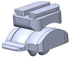
The final modeled CAD assemblies of each of the implants with each of the components labeled are shown in Figure 13.
2.2. ABAQUS Material Properties
The bearing component is made of UHMWPE and the tibial and talar components are made of CoCrMo (Figure 14). The settings for the Elastic behavior of these materials are shown in Table 1. Since the Young’s modulus of CoCrMo is significantly higher than UHMWPE, the Young’s modulus was set from the real value of 210e3 MPa to 210e6 MPa and the Poisson’s ratio was kept the same. This condition is called “Pseudo-Rigid”, which has a very high Young’s modulus to replicate the effect of a rigid body having an infinite stiffness. This significantly decreased run-time and yielded the same results as assigning them as “Deformable” within ABAQUS. It also permitted boundary conditions and loading to be placed on any portions of the metallic components, which would be limited with “Rigid” behavior in ABAQUS since all nodes of a rigid body move with the same motion. For the purposes of our study, the stresses and strains were not of concern on the metallic components. The bearing was modeled as “elastic-plastic” which was assumed in other FEA studies as well [5,19]. This indicates that the elastic behavior is assumed to have a single Young’s modulus and Poisson’s ratio.
In addition to the elastic behavior, plastic behavior was modeled for the UHMWPE to represent the material’s response after yielding. This behavior was extracted from a true stress-strain curve. This curve (Figure 15) was created with data for UHMWPE with a grade of virgin GUR 1020, provided by Miller [25]. This specific true-stress and true strain data has been used consistently in other FEA studies by Martinelli, Zhang, and Yu [5,19,23]. The yield strength for this grade of UHMWPE is 10.86 MPa, which is the lowest value reported in the literature among grades of this polyethylene [26]. This is done for a conservative estimate of von Mises stress on the bearing, predicting yielding earlier than expected. Specifics on the grade of UHMWPE were not provided by the manufacturers. It is also important to note that the Poisson’s ratio of UHMWPE is 0.46, which is close to the incompressible value of 0.5 observed on rubbers. This indicates that minimal volume changes are expected as the material expands laterally and contracts longitudinally under compression.
2.3. ABAQUS Step/Interactions
The analysis step within ABAQUS was defined at a fixed increment for both implants (INBONE II: 0.05, Vantage: 0.01). Utilizing this small step increment ensured proper convergence as the ABAQUS equation solver computed the stiffness matrix to derive stress and strain outputs.
The interactions between components consisted of ties and contacts. Components that have no relative motion between them were tied together, essentially making the two components one piece. For the INBONE II, the tibial tray was tied to the stem subassembly and to the bearing. The talar tray was tied to the pegs and stem. For the Vantage, the tibial tray was tied to the bearing and the locking clip, and the locking clip was tied to the bear-ing. A visualization of the tibial tray to bearing tie interaction is shown in Figure 16. Con-tact interactions are appropriate for surfaces that have sliding relative motion between them and where the pressure between them is relevant. These surfaces were the articulat-ing surfaces of the implant, which were the top bicondylar surface of the talar tray and the bottom bicondylar surface of the bearing. These surfaces and the corresponding settings for this contact interaction were inputted into ABAQUS, as shown in Table 2. The tangen-tial behavior was assumed to be based on a Coulomb friction model. The friction coeffi-cient of μ=-0.04 has been used vastly within TAA FEA studies with CoCrMo and UHMWPE [5,19] and has been benchmarked as the appropriate coefficient in an experi-mental analysis of friction on joint replacement implants performed by Godest [27].
2.4. Implant Loading
Gait and loading data were extracted from the literature. The aim of this study was to evaluate the maximum stress on the implants during the stance phase, as well as the behavior during each of the four subphases of the stance phase of gait. Dorsiflexion/plantarflexion data was collected by Zhang [19,20] on a post-operative INBONE II TAA patient while walking on force plates in a gait lab. This data is plotted with images of the ankle position during the four subphases of gait in Figure 17a. In particular, points of interest are indicated in red for 10%, 20%, 30%, 40%, 49%, and 60%. These characterize the entire spectrum of the stance phase of gait. With the angle for each of these points of interest, six separate CAD models were developed within SolidWorks to rotate the implant. When the ankle is flexed, the tibial component and bearing flex to the corresponding angle while the talar component is stationary. These rotated models are shown next to their corresponding gait percentage on the INBONE II dorsiflexion/plantarflexion angle plot in Figure 17b.
The load used for the INBONE II was the total ankle joint contact force. This contact force was assumed to be purely axial as a compressive load on the tibial component. The axial compressive load on the INBONE II during gait is shown in Figure 18. The same gait percentage points of interest are emphasized in red. This load data, as well as the flexion data, was based on a 50-year-old male patient with weight of 75.3 kg and height of 172 cm, corresponding to a BMI of 25.5 [28]. The maximum load was 4,787 N, which if normalized by the patient’s body weight of 75 kg (736 N), corresponds to a load of 6.5x body weight (BW). This also corresponds to the point of maximum dorsiflexion on the implant.
Maximum load of 4,787 N at 49% gait
The axial compressive load aligned with the axis of the tibial stem (Figure 19a). The load was uniformly distributed across the surfaces of the stem and top of the tibial tray because these are the areas where the implant contacts the bone (Figure 19b). The uniformly distributed load was calculated based on the axial compressive load divided by the summation of areas of the loading surfaces. A local coordinate axis was attached to the front of the tibial component to ensure that the loading and boundary conditions were applied relative to the rotated coordinate system.
The process for determining the loading of the Vantage was similar. Gait and load data were taken based on a healthy ankle from Bell’s [21] experiment on ankle joint prostheses wear, which was used in Martinelli’s [5] study on the Zimmer fixed-bearing implant. The load data was not provided by Exactech [29], however they did reveal the dorsiflexion range of 15 degrees and plantarflexion range of 15 degrees, which is nearly identical to the data used by Martinelli. This data was plotted in Figure 20a, with the subphases of gait and points of interest indicated on the plot. These points of interest were 10%, 20%, 30%, 40%, 50% and 60% gait. Images of the six rotated Vantage CAD models are shown next to their corresponding gait percentages on the dorsiflexion/plantarflexion plot in Figure 20b.
The axial load data also taken from Bell’s [21]. This is plotted in Figure 21 with a maximum load of 3,158 N at 40% gait.
The resultant axial load was applied along the axis of the central peg of the tibial tray (Figure 22a). The loading among the pegs was computed using a statically indeterminate approach. The internal loads within the pegs were calculated based on the resultant axial load and compatibility relations. The forces in each peg were calculated in a MATLAB script using a system of three linear equations for all gait percentages of interest. The corresponding load per peg was uniformly distributed on the top of the pegs’ surfaces as shown in Figure 22b. A local coordinate system was attached to the side of the tibial component.
2.5. ABAQUS Boundary Conditions
Boundary conditions were considered based on two primary conditions. The implant was constrained based on how the implant interfaces with the bone. It was assumed that there was no loosening of the implant from the bone. Rigid body modes were eliminated in placing these constraints. For both implants, the bottom of the talar component was constrained with rollers to restrict vertical translations. To constrain lateral translations, pins were generally placed on the center of the pegs. For the INBONE II, the top of the mid stem and the bottom of the pegs on the talar component were pin constrained. For the Vantage, the top of the small tibial pegs, edges of the large tibial peg, and the bottom of the talar pegs were pin constrained. Boundary conditions placed on the tibial pegs were defined relative to the local coordinate system since the tibial component rotated based on the ankle angle for the corresponding gait percentage. By pin constraining the implant, rigid body modes were eliminated. The element type used in meshing is a linear tetrahedral element that has only 3 translational degrees of freedom per node. However, by constraining the translational degrees of freedom, translational and rotational rigid body modes were constrained. Examples of the roller and pin constraints are shown for the INBONE II (Figure 23) and Vantage (Figure 24).
2.6. ABAQUS Meshing
The element type used for meshing was C3D4, which is a 4 noded linear tetrahedron element. ABAQUS free meshing was utilized to mesh these elements. These have been used consistently across TAA studies [23,30]. They are appropriate for regions of fine meshes and are computationally efficient. In particular, the surfaces in contact were meshed finely with local seeding for accurate results. A convergence study was done on the middle of the articulating surface of the bearing, as shown in the top row of Figure 25. The von Mises stress and contact pressure were evaluated in this region for seed sizes of 5, 3, 1, 0.75, 0.65, and 0.50 mm. Convergence was determined by comparing the results from one seed size to the lowest seed size (0.50 mm). If the results for von Mises were within 1% and the results for contact pressure were within 5%, the mesh was determined to have converged. For the INBONE II, this was reached at a seed size of 0.75 mm (48,102 DOF) and for the Vantage, this was reached at 0.65 mm (33,294 DOF). A side-by-side summary of the mesh convergence study for both implants is shown in Figure 25.
3. Results
Results were collected for the von Mises stress and contact pressure on the articulating surface of the bearing to investigate the mechanical performance of the implant’s weakest component during stance.
3.1. von Mises Stress
The von Mises stress is a metric for determining the equivalent stress for ductile materials. It is a failure criterion when comparing the equivalent stress to the yield strength. The safety factor quantifies how close the material is to yielding. It was important to investigate the maximum von Mises stress on the implants to find how close the UHMWPE was to yielding under the load applied.
The maximum von Mises stresses for both implants occurred in the regions of thin-nest bearing, which was the middle of each condyle on the articulating surface. The stress distributions were uniform across both condyles (Figure 26). Both of the implants plas-tically deformed and yielded since their maximums were above the yield strength for the material (10.86 MPa). As mentioned earlier, this yield strength is the most conservative es-timate since it is the lowest value reported in the literature [26].
The stress results for all 6 gait configurations for the INBONE II are tabulated in Table 3 and shown in Figure 27. The compressive load increased from 10-50% gait, and the von Mises stress increased correspondingly. The maximum stress occurred at 49% gait, which is during the terminal stance phase of gait. During pre-swing, the load and corresponding stress decreased significantly. Uniformity was maintained on both condyles of the bearing with maximum values on the middle of the bearing surface. The maximum values of each configuration are indicated.
The stress distributions for all 6 gait configurations for the Vantage are tabulated in Table 4 and shown in Figure 28. The compressive load increased from 10-40% gait, and the von Mises stress increased correspondingly. The maximum stress occurred at 40% gait, during the terminal stance phase of gait. Around 50%, however, the load and corresponding stress decreased significantly. Again, uniformity was seen on either condyle of the bearing with maximum values in the expected areas. The maximum values of each configuration are indicated.
3.2. Contact Pressure
Contact pressure is defined as the contact normal force on each element divided by the contact area between two bodies. In our study it was calculated to determine the amount of pressure applied between the stiffer CoCrMo talar component on the softer UHMWPE bearing, as well as the friction between the two surfaces. This was utilized to evaluate bearing wear rate. The maximum contact pressure for both implants is shown in Figure 29. The central area of the bearing exhibited high congruence and conformity with the talar component, and also experienced the highest von Mises stress and highest uniform contact pressure.
Our modeling also identified edge loading at specific angles. At a dorsiflexion angle of 32, the INBONE II bearing component was noted to sit slightly anterior to the talar component. This led to the talar component anterior edge which was in contact with the bearing to sustain contact pressures over twice as high as the uniform maximum contact pressure.
Similarly, the Vantage implant exhibited edge loading on the posteroinferior aspect of the bearing surface. Additionally, the posterior tibial peg sustained a distributed load twice as large as the anterior pegs (73 MPa vs. 48 MPa), leading to high contact normal forces and contact pressures on the edge of the bearing surface in these areas. This edge maximum was over three times larger than the uniform maximum.
The contact pressure results for all 6 gait configurations for the INBONE II are tabulated in Table 5 and shown in Figure 30. As the uniformly distributed pressure load increased, the contact pressure increased.
The contact pressure results for all 6 gait configurations for the Vantage are tabulated in Table 6 and shown in Figure 31. Similar to the INBONE II, as compressive load and dorsiflexion angle increased, the contact pressure increased. The edge effect was visible throughout the entire gait cycle since the posterior peg loading was higher than the anterior pegs.
4. Discussion
4.1. Indications of Results
In both implants the highest von Mises stress was observed on the condyles in the central region of the bearing. These regions corresponded to the areas where the bearing in thinnest. It is biomechanically and clinically important to recognize that the stress is magnified in these regions.
In the Vantage, the load is transmitted through the pegs, through the thin region of the tibial tray, and onto the superior surface of the bearing (Figure 32a). In the frontal cross-sectional cut (normal to the X’ axis) at the midplane of the bearing, the smallest thickness of the bearing is indicated by t, and it lies along the condylar radius of the bearing. Stress concentrations at the sharp corners of the bearing were identified, circled in red, where the stress propagates as it reaches the condylar radii. In the region shown in green, the highest stresses are seen by the bearing (10-15 MPa). A medial view of the bearing with a cross-sectional cut (normal to the Z’-axis) at the region of smallest thickness is shown in Figure 32b. This thickness t, is smallest at the middle of the medial radius. The same principle occurs for the lateral radius since the stress is symmetric on either condyle of the bearing. The corresponding highest regions of stress on the bearing are circled in yellow in a view with multiple cross-sectional cuts in Figure 32c.
At these regions where the bearing is thinnest, high magnitudes of contact normal forces exist. The uniform maximum contact pressure distributions exist in these regions, making them most vulnerable to linear wear and pitting.
Similarly, the regions where edge effect was identified on the bearing surface are most susceptible to accelerated wear. For the INBONE II, the edge effect starts on the anterior aspect of the bearing around 30% of the stance phase or at 22.7° DF. It is important to note that average maximum clinical dorsiflexion values are no more than 20°. A clinical trial by Mulcahy [31] reported average dorsiflexion of patients after receiving an INBONE II to be 14.3°. Therefore the anterior edge loading noted at greater dorsiflexion angles are unlikely to be experienced in vitro.
4.2. Unloading and Reloading
This study only loaded implants once, and since yielding occurred, it would be important to investigate the effect of unloading and reloading the materials. The maximum plastic strain occurred on the bearing surface and occurred at the region of maximum von Mises stress. When unloaded (Figure 33a), the material would incur a permanent plastic deformation and an elastic recovery strain. As the material is re-loaded (Figure 33b), it would load at the permanent set until it reached the true strain corresponding to the elastic recovery strain, raising the yield strength. The new yield strength would correspond to the true strain corresponding to the maximum plastic strain at the maximum von Mises stress location (Figure 33c). This repeats with each gait cycle in a strain-hardening process.
4.3. Comparison to other Studies
Direct comparison to other studies was not possible due to limitations of this study. Other studies included different components within their models, including bone or soft tissue. However, general agreement was seen between these other studies and the present work.
The INBONE II model was compared to Yu’s [23] study on the INBONE II. Despite their incorporation of the entire foot with the implant in their model, the von Mises stress on the INBONE II was noted to be 15 MPa, only a 12% difference to the results of this study. Similarly slight uniformity across condyles of the stress on the bearing was noted, consistent with this work.
Zhang [19] performed a comparative FEA study in ABAQUS of three different TAA implants, including the Wright INBONE II. He post-processed gait data from TAA patients with these implants using a multibody dynamics modeling (MSK-MBD) software [20]. A comparison of our contact pressure results found the edge effect of the contact pressure, with a magnitude of 41 MPa, only a 5% difference. There was strong uniformity across both condyles in their model, however, the maximum value in the uniform region was higher by 24% (21 MPa).
Our analysis of the Vantage is unique in that there are no existing FEA studies for this implant within the literature. To the author’s knowledge, this is the first study with open access to the community. With this limitation, comparison was done against other implants, which are similar in geometry. The results of the von Mises stress were compared to Martinelli’s [5] work on the Zimmer fixed-bearing implant, from which the gait and load data for the Vantage were taken from. The stress observed by Martinelli was 17% higher (14 MPa), however uniformity was observed on either condyle of the bearing. A similar implant to the Vantage, with multiple pegs on the tibial component, was custom designed by Elliot [32] and the difference in stress magnitude was a mere 4%. For contact pressure, uniformity was seen on either condyle of the bearing in Martinelli’s work, and the edge effect was observed in Rodrigues’ [30] work on the Agility implant, and was 14% higher in magnitude (45 MPa). Despite the limitations and simplicity of this study, there is still reasonable agreement within 25% among most of these studies mentioned.
4.4. Future Recommendations
Future improvements on this work should implement several facets so that the FEA model is more reflective of in vitro implant interaction with surrounding anatomy.
It was difficult to model the geometry of the implants precisely due to lack of manufacturer provided specifications. One alternative method of obtaining these dimensions would be to measure sizes off CT scans of patients with these implants within ABAQUS. Adjacent patient bony geometry could also be obtained from this imaging, such as done by Zhang et al for the INBONE II [19].
For the INBONE II, it would be clinically relevant to examine the effect of having longer and shorter stems within the model. With longer stem lengths, buckling becomes a concern, and consequent implant loosening from the bone. For both implants, it would be most relevant to test all sizes of the implant that the manufacturer specifies to accurately capture the effect of the implant across the full spectrum of patients.
There are different grades of UHMWPE that vary in yield strength and Young’s modulus [26]. The precise grade of UHMWPE should be obtained from the manufacturers to ensure accuracy of results and yielding predictions. However, for the most conservative estimates, the current yield strength should be used still (10.86 MPa).
In general, C3D4 linear tetrahedron elements are too stiff for 3D structural analysis. A linear approximation cannot be applied to curved surfaces unless many individual elements are used to approximate the displacement, as used in this study. This analysis could be improved by using C3D10M elements, which are modified quadratic tetrahedron elements. Quadratic elements have a quadratic shape function approximation for displacement between two nodes. This yields closer precision for elements that are on curved surfaces. Remeshing would need to be considered within the components that do not have a contact interaction in order to run this simulation within the 250,000 node limit of the ABAQUS Teaching License provided by the university.
The tibial and talar bone adjacent to the implants is cancellous, trabecular bone. A better assumption than attaching the talar component to this bone with rollers would be to use nonlinear one-dimensional springs.
Additionally, during gait the loading is not truly uniform. There is asymmetric loading across the implant due to shear and lateral loading. Although axial loading is ten times higher than shear loading, it would still be relevant to include these shear and lateral loads to determine whether they contribute to aseptic loosening.
Currently, there is limited clinical data on long term 15-20 year implant longevity. This could be predicted by performing a wear analysis using Hertzian contact mechanics on the bearing to calculate amount of linear wear over millions of cycles. Additionally, Paris’ equation could be used to better understand fracture mechanics and predict likelihood of subsurface bearing cracking over time.
5. Conclusions
In this study, the results for von Mises stress and contact pressure indicated a great amount of uniformity on either condyle of the bearing articulating surface. Although there were limitations to this model in the number of components utilized, our results demonstrated close agreement to the previous literature.
With uniformly distributed loading, the highest magnitudes occurred in areas of thinnest bearing. Unsurprisingly, higher compressive load led to higher stresses experienced by the implant. Increased ankle dorsiflexion angles were also correlated to higher loads and stress experienced at the bearing surface. Clinically this raises a question of how increased body weight affects these patterns, and whether there is a threshold BMI above which there should be a concern for unacceptably accelerated bearing wear.
The axial compressive load, which is transferred through the distal tibia, acted axially on the tibial component and acted normal to the pegs or surfaces. In the maximum load cases for the von Mises stress, the safety factor was calculated to be below 1 when compared to the yield strength of 10.86 MPa. This indicates that the material plastically deformed under these conditions and the yield strength was raised to the true stress corresponding to the true strain from the plastic deformation. In the uniform regions, the contact area between the bearing and talar components demonstrated close congruency.
In certain configurations, the contact pressure revealed concentrated areas of increased magnitude consistent with edge loading. This raises clinical concern for focal areas of increased wear, and possible subsurface bearing cracking.
Our work contributes to the body of data available on TAA biomechanics and implant wear patterns, laying the foundation for future research to better understand implant longevity and improve patient outcomes.
Author Contributions
Conceptualization, T.S.J, N.N, and J.R; methodology, T.S.J, J.R, and S.H; software, T.S.J, J.R, and S.H; validation, T.S.J, J.R, and S.H; formal analysis, T.S.J, J.R, and S.H; investigation, T.S.J, M.N, and J.R; resources, M.N and N.N; data curation, T.S.J, M.N, and J.R; writing—original draft preparation, T.S.J; writing—review and editing, T.S.J, M.N, and J.R; visualization, T.S.J and J.R; supervision, M.N, J.R and N.N; project administration, M.N All authors have read and agreed to the published version of the manuscript.
Funding
This research received no external funding.
Institutional Review Board Statement
Not applicable.
Informed Consent Statement
Not applicable.
Data Availability Statement
We encourage all authors of articles published in MDPI journals to share their research data. In this section, please provide details regarding where data supporting reported results can be found, including links to publicly archived datasets analyzed or generated during the study. Where no new data were created, or where data is unavailable due to privacy or ethical restrictions, a statement is still required. Suggested Data Availability Statements are available in section “MDPI Research Data Policies” at https://www.mdpi.com/ethics. https://digitalcommons.calpoly.edu/theses/2766/
Acknowledgments
We would like to express our special thanks to the following colleagues for their contributions which made this research possible. Mason Kaseeska from Cal Poly IT department for assistance in the remote desktop for running ABAQUS. Erik Hallgrimson, a current Cal Poly ME undergraduate student for helping with the design the components of the Vantage model. Dr. Nicolo Martinelli (Orthopedic Surgeon atof Instituto Ortopedico Galeazzi, Milan, Italy) for granting permission to use the gait and load data from his study to use for the Exactech Vantage. Dr. Yanwei Zhang (Xi’an Jiaotong University, X’ian, China) for providing gait and load data and a reference model of the bearing for the Wright Medical INBONE II. Prf. Stephen Klisch (Cal Poly, San Luis Obispo, CA, USA) for providing biomechanics and continuum mechanics advice for the appropriate model setup.
Conflicts of Interest
The authors declare no conflicts of interest.
References
- “Ankle Joint,” Cleveland Clinic. Available online: https://my.clevelandclinic.org/health/body/24909-ankle-joint (accessed on 28 July 2023).
- “Anatomy of the Ankle,” Southern California Orthopedic Institute. Available online: https://www.scoi.com/specialties/ankle-doctor/anatomy-ankle (accessed on 28 July 2023).
- Brockett, C.L.; Chapman, G.J. Biomechanics of the ankle. 2016. [Google Scholar] [CrossRef] [PubMed]
- Pappas, M.J.; Buechel, F.F. Failure Modes of Current Total Ankle Replacement Systems. Clinics in Podiatric Medicine and Surgery 2013, 30, 123–143. [Google Scholar] [CrossRef]
- Martinelli, N.; et al. Contact stresses, pressure and area in a fixed-bearing total ankle replacement: A finite element analysis. BMC Musculoskelet Disord 2017, 18. [Google Scholar] [CrossRef]
- Gil-Castillo, J.; Alnajjar, F.; Koutsou, A.; Torricelli, D.; Moreno, J.C. Advances in neuroprosthetic management of foot drop: A review. Journal of NeuroEngineering and Rehabilitation. [CrossRef] [PubMed]
- “Arthritis of the Foot and Ankle,” American Academy of Orthopedic Surgeons. Available online: https://orthoinfo.aaos.org/en/diseases--conditions/arthritis-of-the-foot-and-ankle/ (accessed on 28 July 2023).
- Coester, L.M.; Saltzman, C.L.; Leupold, J.; Pontarelli, W. Long-Term Results Following Ankle Arthrodesis for Post-Traumatic Arthritis. 2001. www.jbjs.org.
- DeOrio, J.K.; Nunley, J.A.; Easley, M.E.; Valderrabano, V. Vantage Total Ankle Fixed Bearing Operative Technique.
- A New Perspective in Total Ankle: Vantage Total Ankle. 2019.
- Baena, J.C.; Wu, J.; Peng, Z. Wear performance of UHMWPE and reinforced UHMWPE composites in arthroplasty applications: A review. Lubricants 2015, 3, 413–436. [Google Scholar] [CrossRef]
- Patil, N.A.; Njuguna, J.; Kandasubramanian, B. UHMWPE for biomedical applications: Performance and functionalization. European Polymer Journal 2020, 125, 109529. [Google Scholar] [CrossRef]
- Noori, N.B.; Ouyang, J.Y.; Noori, M.; Altabey, W.A. A Review Study on Total Ankle Replacement. Applied Sciences 2022, 13, 535. [Google Scholar] [CrossRef]
- Jones, M.D.; Buckle, C.L. How does aseptic loosening occur and how can we prevent it?
- “Frequently Asked Questions about Total Ankle Replacement,” Washington University Orthopedics. Available online: https://www.ortho.wustl.edu/content/Education/2915/Patient-Education/Educational-Materials/Total-Ankle-Replacements-FAQs.aspx#:~:text=While%20results%20at%205%20and,years%20after%20the%20original%20surgery (accessed on 13 March 2024).
- Kofoed, H.; Stiirup, J. Comparison of ankle arthroplasty and arthrodesis.
- Glazebrook, M.; Burgesson, B.N.; Younger, A.S.; Daniels, T.R. Clinical outcome results of total ankle replacement and ankle arthrodesis: a pilot randomised controlled trial. Foot and Ankle Surgery 2021, 27, 326–331. [Google Scholar] [CrossRef] [PubMed]
- Hauer, G.; et al. Revision Rates After Total Ankle Replacement: A Comparison of Clinical Studies and Arthroplasty Registers. Foot Ankle Int 2022, 43, 176–185. [Google Scholar] [CrossRef] [PubMed]
- Zhang, Y.; et al. Comparison of joint load, motions and contact stress and bone-implant interface micromotion of three implant designs for total ankle arthroplasty. Comput Methods Programs Biomed 2022, 223, 106976. [Google Scholar] [CrossRef]
- Zhang, Y.; Chen, Z.; Zhao, H.; Liang, X.; Sun, C.; Jin, Z. Musculoskeletal modeling of total ankle arthroplasty using force-dependent kinematics for predicting in vivo joint mechanics. Proc Inst Mech Eng H 2020, 234, 210–222. [Google Scholar] [CrossRef] [PubMed]
- Bell, C.J.; Fisher, J. Simulation of polyethylene wear in ankle joint prostheses. J Biomed Mater Res B Appl Biomater 2007, 81, 162–167. [Google Scholar] [CrossRef] [PubMed]
- “INBONE Total Ankle System,” Wright Medical Total Ankle Institute. Available online: http://www.totalankleinstitute.com/inbone-products/inbone-ankle/ (accessed on 22 August 2023).
- Yu, J.; et al. Finite element stress analysis of the bearing component and bone resected surfaces for total ankle replacement with different implant material combinations. BMC Musculoskelet Disord 2022, 23, 1–11. [Google Scholar] [CrossRef] [PubMed]
- Zhang, Y.; Chen, Z.; Zhao, D.; Yu, J.; Ma, X.; Jin, Z. Articular geometry can affect joint kinematics, contact mechanics, and implant-bone micromotion in total ankle arthroplasty. Journal of Orthopaedic Research 2023, 41, 407–417. [Google Scholar] [CrossRef] [PubMed]
- Miller, M.C.; Smolinski, P.; Conti, S.; Galik, K. Stresses in polyethylene liners in a semiconstrained ankle prosthesis. J Biomech Eng 2004, 126, 636–640. [Google Scholar] [CrossRef] [PubMed]
- Malito, L.G.; Arevalo, S.; Kozak, A.; Spiegelberg, S.; Bellare, A.; Pruitt, L. Material properties of ultra-high molecular weight polyethylene: Comparison of tension, compression, nanomechanics and microstructure across clinical formulations. 2018.
- Godest, A.C.; Beaugonin, M.; Haug, E.; Taylor, M.; Gregson, P.J. Simulation of a knee joint replacement during a gait cycle using explicit finite element analysis. 2002.
- “Calculate Your Body Mass Index,” National Institute of Health. Available online: https://www.nhlbi.nih.gov/health/educational/lose_wt/BMI/bmi-m.htm (accessed on 10 March 2024).
- Nunley, J.M.M.; Valderrabano, V.M.P.; DeOrio, J.M.; Easley, M.M. Vantage Ankle Design Rationale. Exactech Extremities.
- Rodrigues, D. Biomechanics of the Total Ankle Arthroplasty: Stress Analysis and Bone Remodeling.
- Mulcahy, H.; Chew, F.S. Current Concepts in Total Ankle Replacement for Radiologists: Features and Imaging Assessment. American Journal of Roentgenology 2015, 205, 1038–1047. [Google Scholar] [CrossRef]
- Jay Elliot, B.; Gundapaneni, D.; Goswami, T. Finite element analysis of stress and wear characterization in total ankle replacements. J Mech Behav Biomed Mater 2014, 34, 134–145. [Google Scholar] [CrossRef]
- Timothy S. Jain, Finite Element Analysis of The Bearing Component of Total Ankle Replacement Implants during The Stance Phase of Gait, California Polytechnic State University, San Luis Obispo, https://digitalcommons.calpoly.edu/theses/2766/.
- Grimston, S.K.; Nigg, B.M.; Hanley, D.A.; Engsberg, J.R. Differences in ankle joint complex range of motion as a function of age. Foot Ankle Int 1993, 14, 215–222. [Google Scholar] [CrossRef]
- Stauffer, R.N.; Chao, E.Y.; Brewster, R.C. Force and motion analysis of the normal, diseased, and prosthetic ankle joint. Clin Orthop Relat Res 1977, 127, 189–196. [Google Scholar] [CrossRef]
- Dekker, T.J.; Hamid, K.S.; Federer, A.E.; et al. The value of motion: patient-reported outcome measures are correlated with range of motion in total ankle replacement. Foot Ankle Spec 2018, 11, 451–456. [Google Scholar] [CrossRef]
- Anil, U.; Singh, V.; Schwarzkopf, R. Diagnosis and detection of subtle aseptic loosening in total hip arthroplasty. The Journal of Arthroplasty 2022, 37, 1494–1500. [Google Scholar] [CrossRef] [PubMed]
Figure 1.
Schematic of the ankle joint [2].
Figure 1.
Schematic of the ankle joint [2].
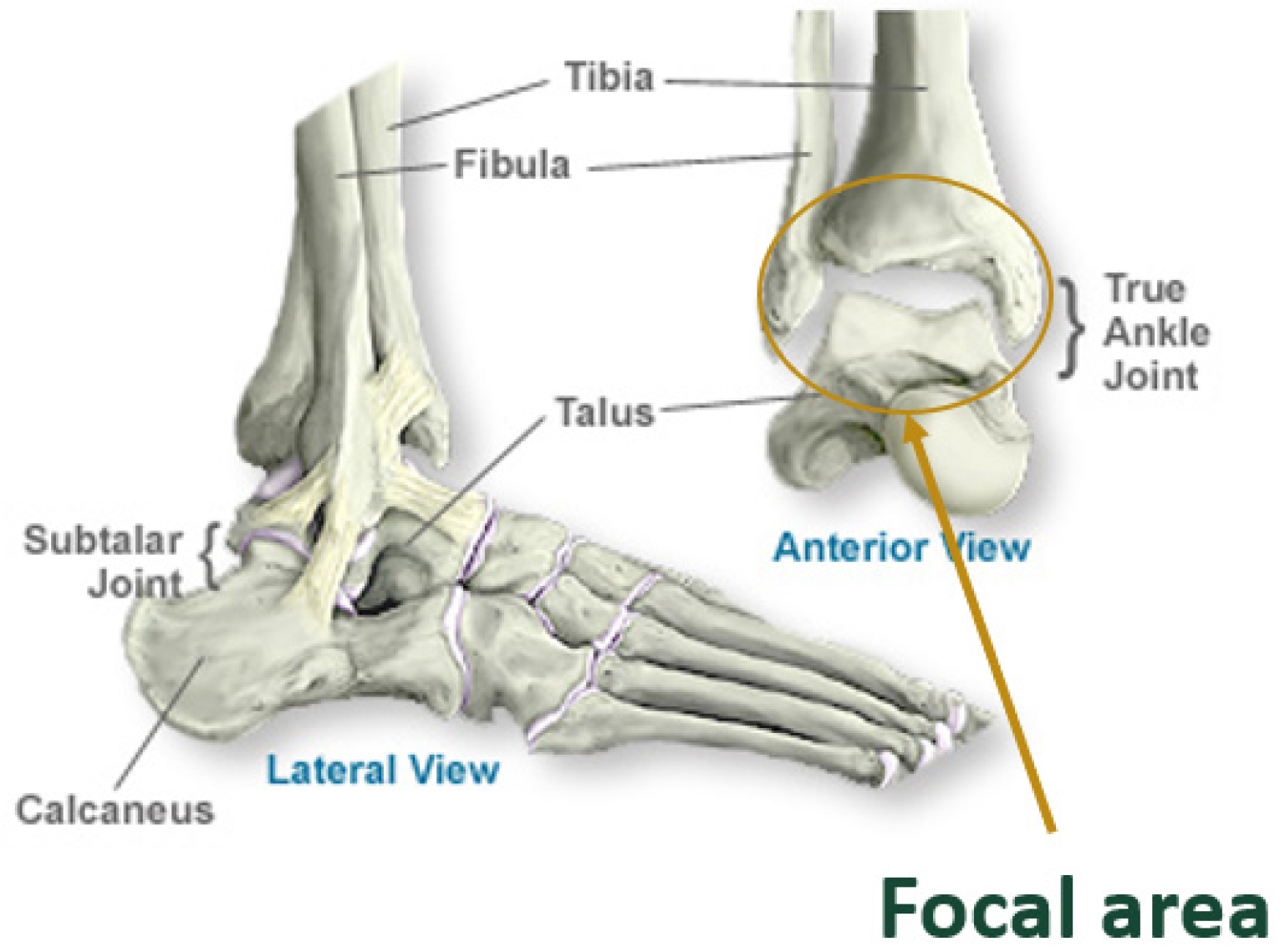
Figure 2.
Ankle planes of motion, with emphasis on dorsiflexion/plantarflexion [4] Licensed permission for use granted by Elsevier.
Figure 2.
Ankle planes of motion, with emphasis on dorsiflexion/plantarflexion [4] Licensed permission for use granted by Elsevier.
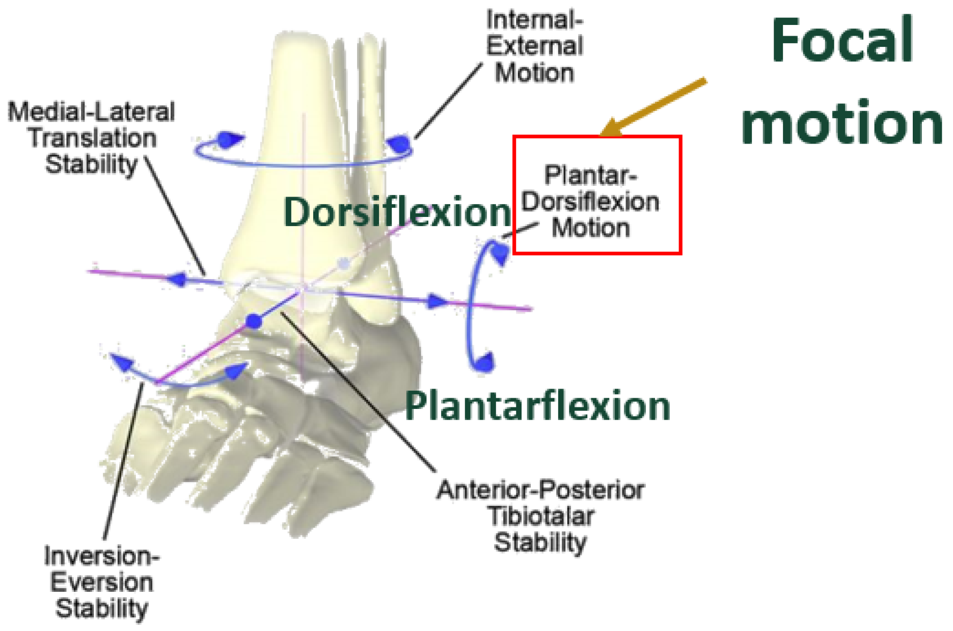
Figure 3.
Subphases of the stance phase of gait [6] Used with permission from BioMed Central under Creative Commons Attribution 4.0.
Figure 3.
Subphases of the stance phase of gait [6] Used with permission from BioMed Central under Creative Commons Attribution 4.0.
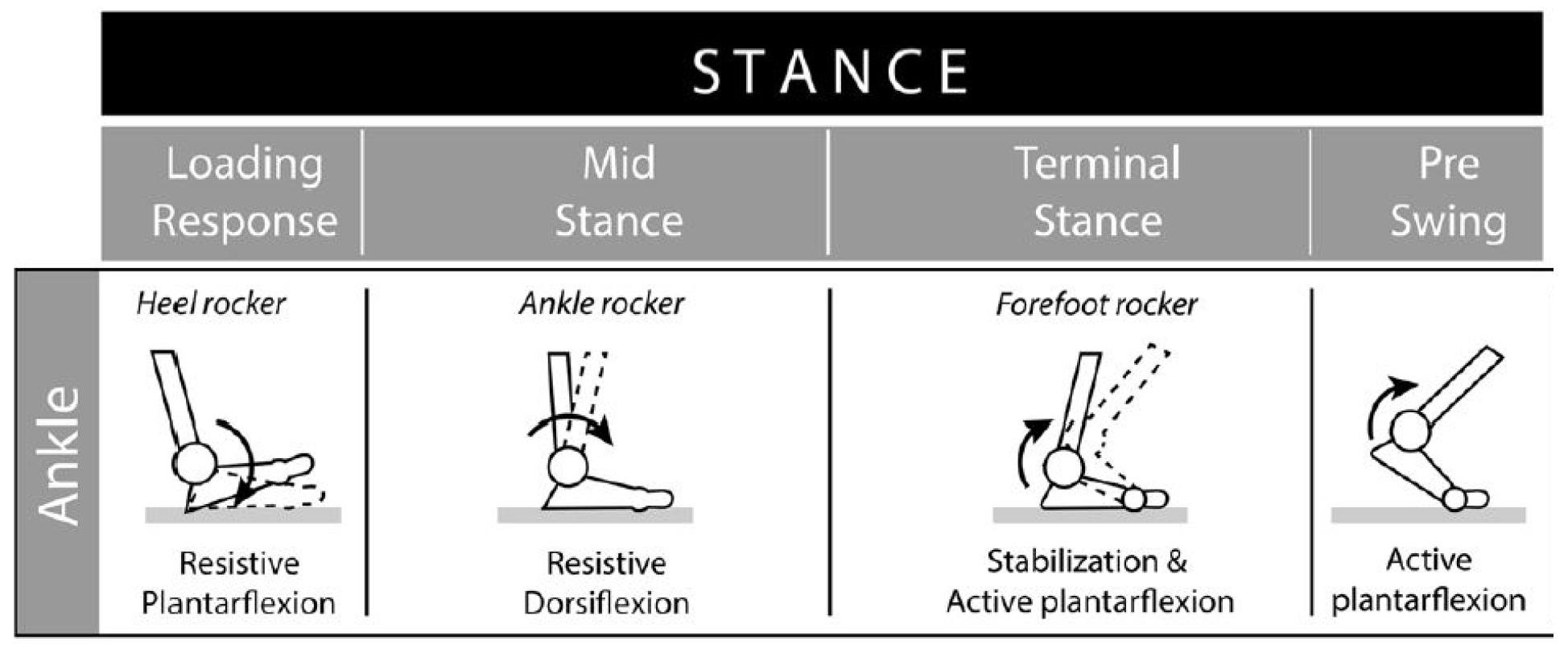
Figure 4.
Dorsiflexion/plantarflexion gait data of a healthy ankle during stance. Figure created by author with healthy ankle data of Martinelli’s [5] study. Permission granted through BMC Musculoskeletal Disorders with Creative Commons Attribution 4.0
Figure 4.
Dorsiflexion/plantarflexion gait data of a healthy ankle during stance. Figure created by author with healthy ankle data of Martinelli’s [5] study. Permission granted through BMC Musculoskeletal Disorders with Creative Commons Attribution 4.0
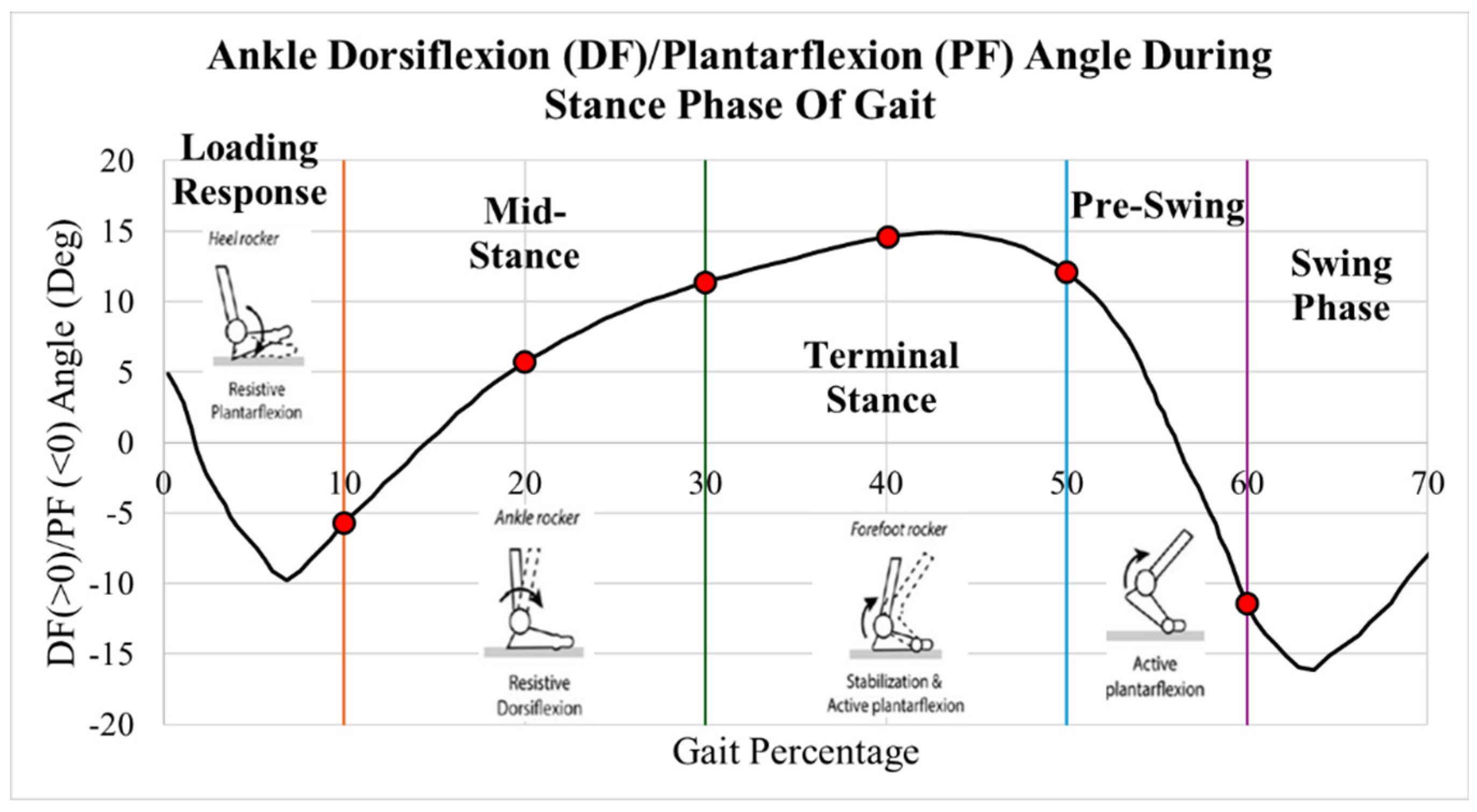
Figure 5.
Labeled diagram of Vantage TAA implant [10]
Figure 5.
Labeled diagram of Vantage TAA implant [10]
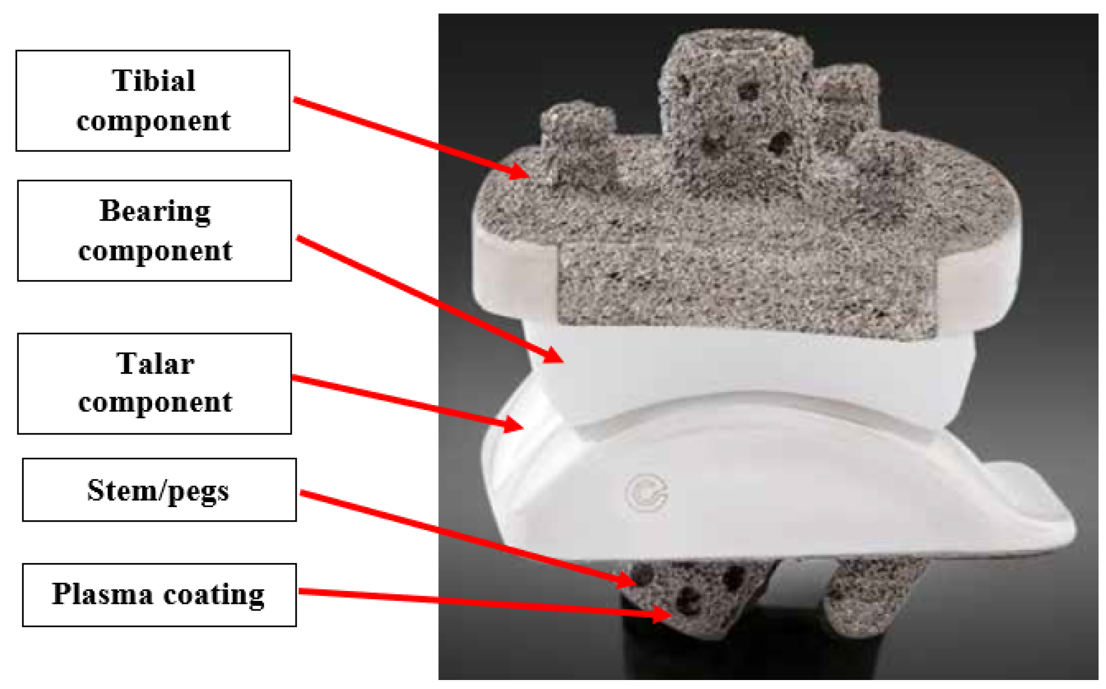
Figure 6.
Labeled locations of failure modes on TAA implant [10]
Figure 6.
Labeled locations of failure modes on TAA implant [10]
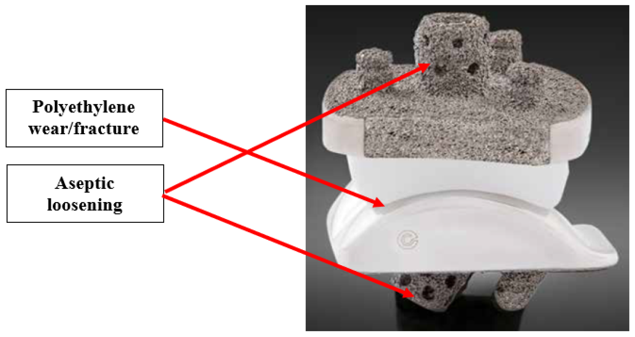
Figure 7.
Focal implants of this study. (a) Wright Medical INBONE II [22], (b) Exactech Vantage [10]
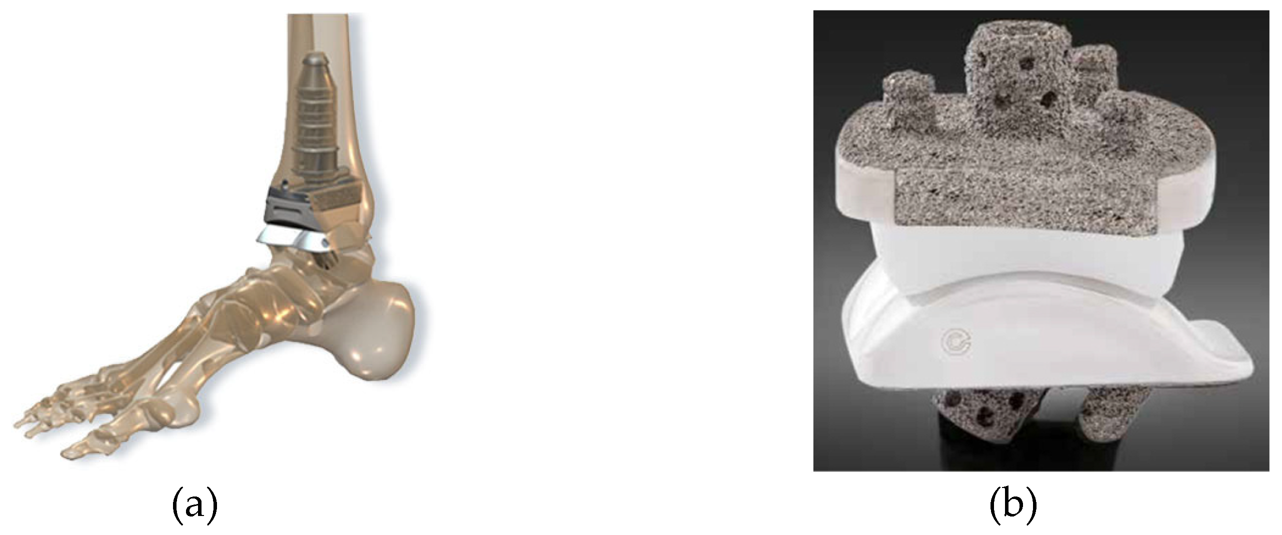
Figure 8.
Long term benefits of FEA structural analysis on TAA implants.
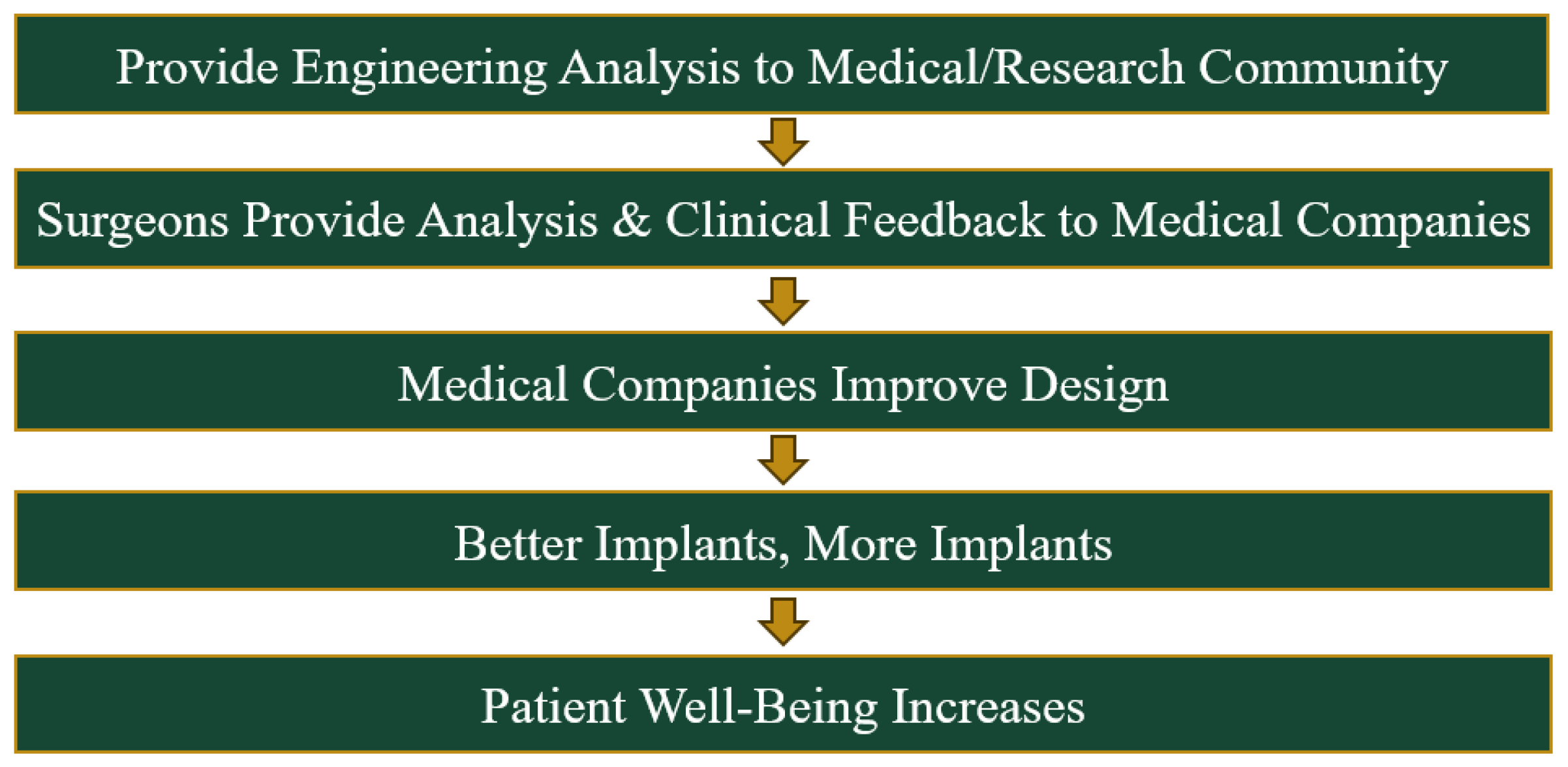
Figure 9.
Methodology of FEA model setup.
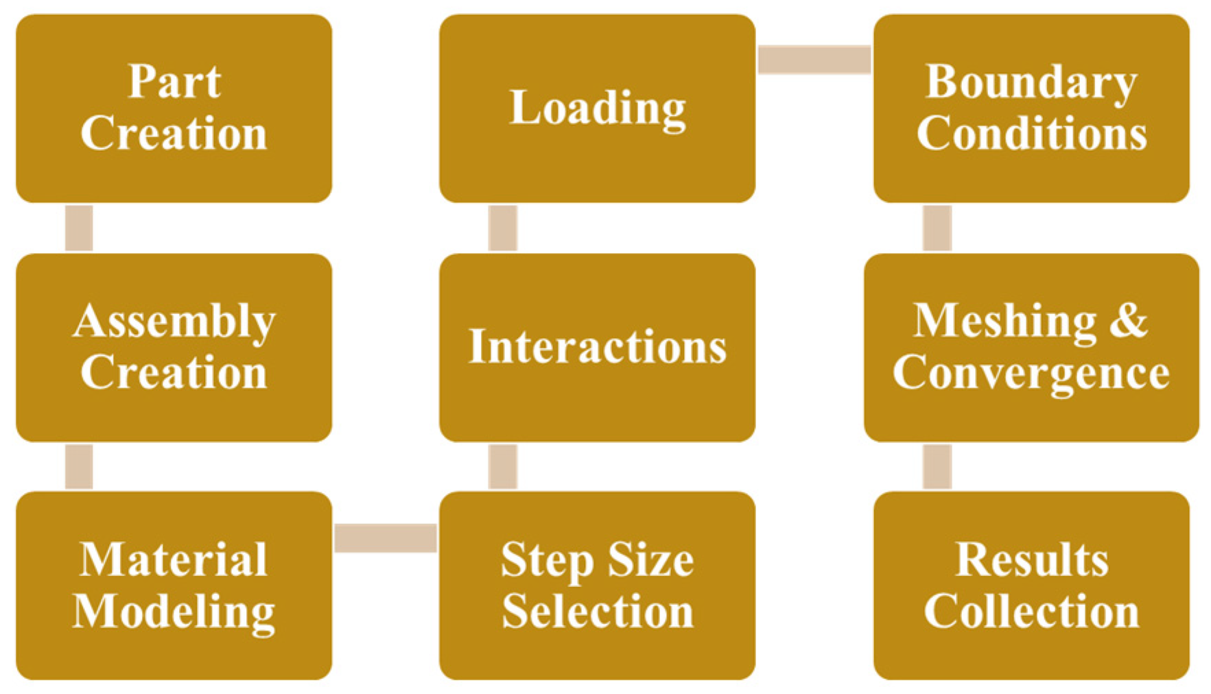
Figure 10.
Geometry modeling process for implant components. (a) Limited dimensions provided by implant manufacturer, (b) DXF of component as a sketch, (c) Adjustments made and extruded CAD components.
Figure 10.
Geometry modeling process for implant components. (a) Limited dimensions provided by implant manufacturer, (b) DXF of component as a sketch, (c) Adjustments made and extruded CAD components.
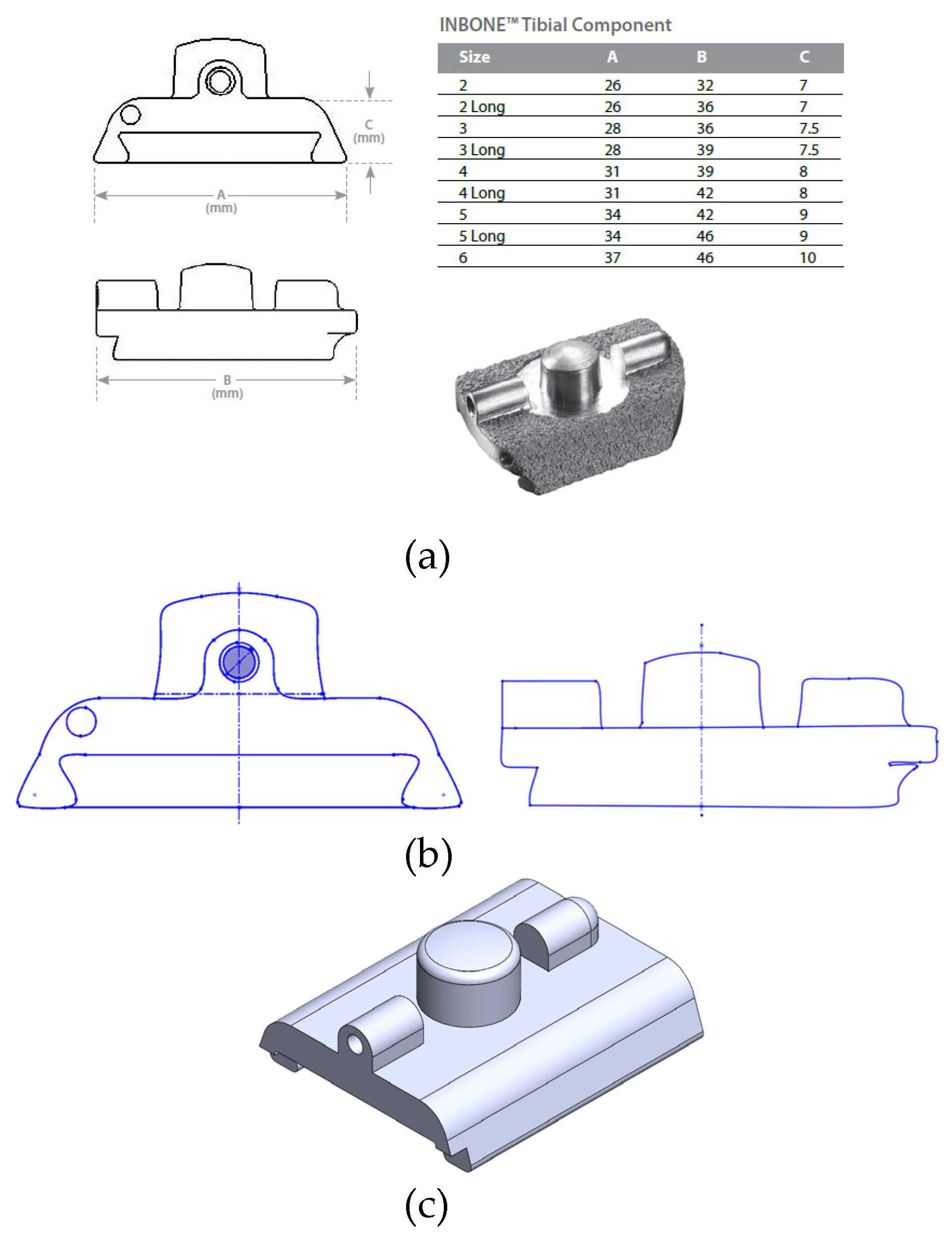
Figure 11.
Important radii for congruency of INBONE II articulating surfaces. (a) Bearing condylar radii, (b) Bearing medial radius, (c) Talar component condylar radii, (d) Talar component medial radius.
Figure 11.
Important radii for congruency of INBONE II articulating surfaces. (a) Bearing condylar radii, (b) Bearing medial radius, (c) Talar component condylar radii, (d) Talar component medial radius.
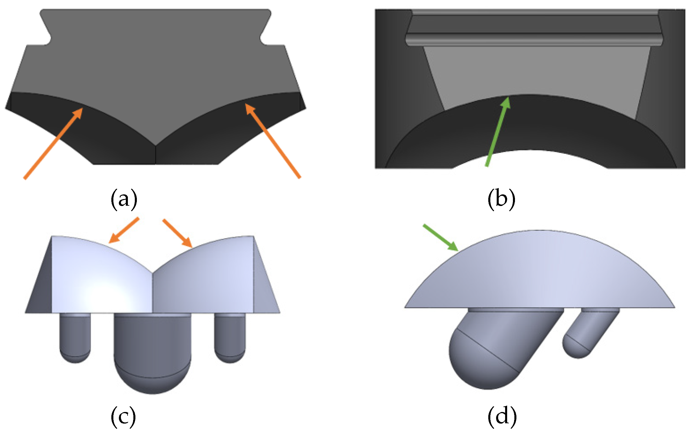
Figure 12.
Important radii for congruency of Vantage articulating surfaces. (a) Bearing condylar radii, (b) Bearing medial radius, (c) Talar component condylar radii, (d) Talar component medial radius.
Figure 12.
Important radii for congruency of Vantage articulating surfaces. (a) Bearing condylar radii, (b) Bearing medial radius, (c) Talar component condylar radii, (d) Talar component medial radius.
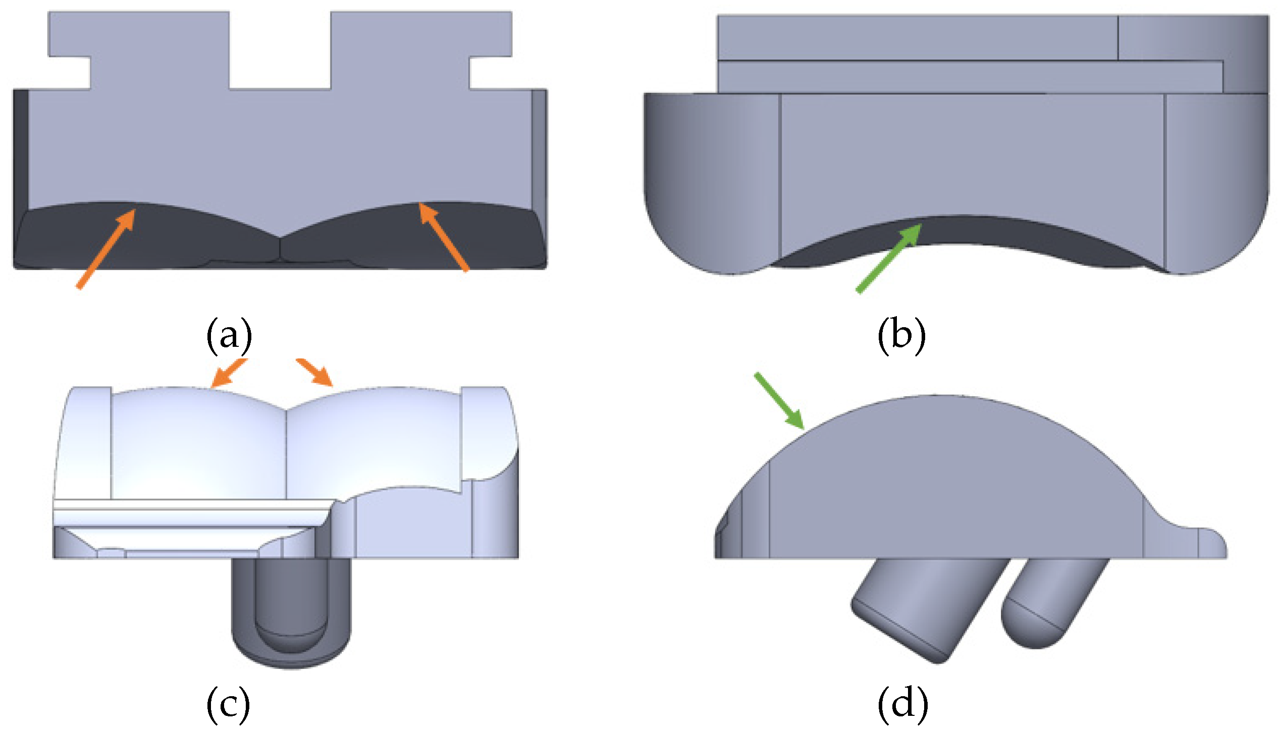
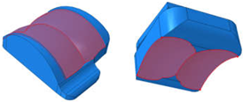
Figure 13.
Labeled assembly for both implants in study. (a) INBONE II, (b) Vantage.
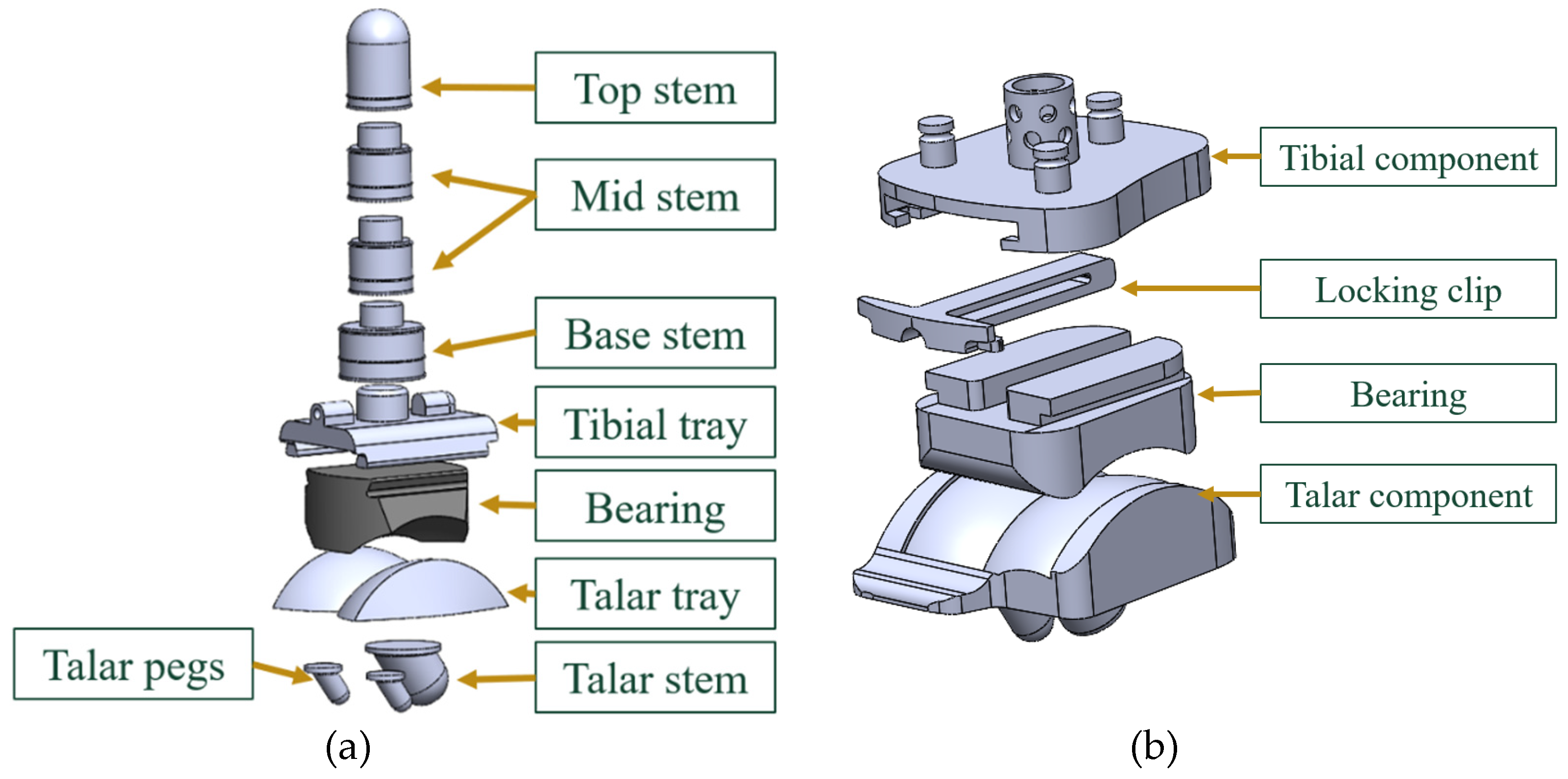
Figure 14.
Material assignments for both the (a) INBONE II and (b) Vantage.
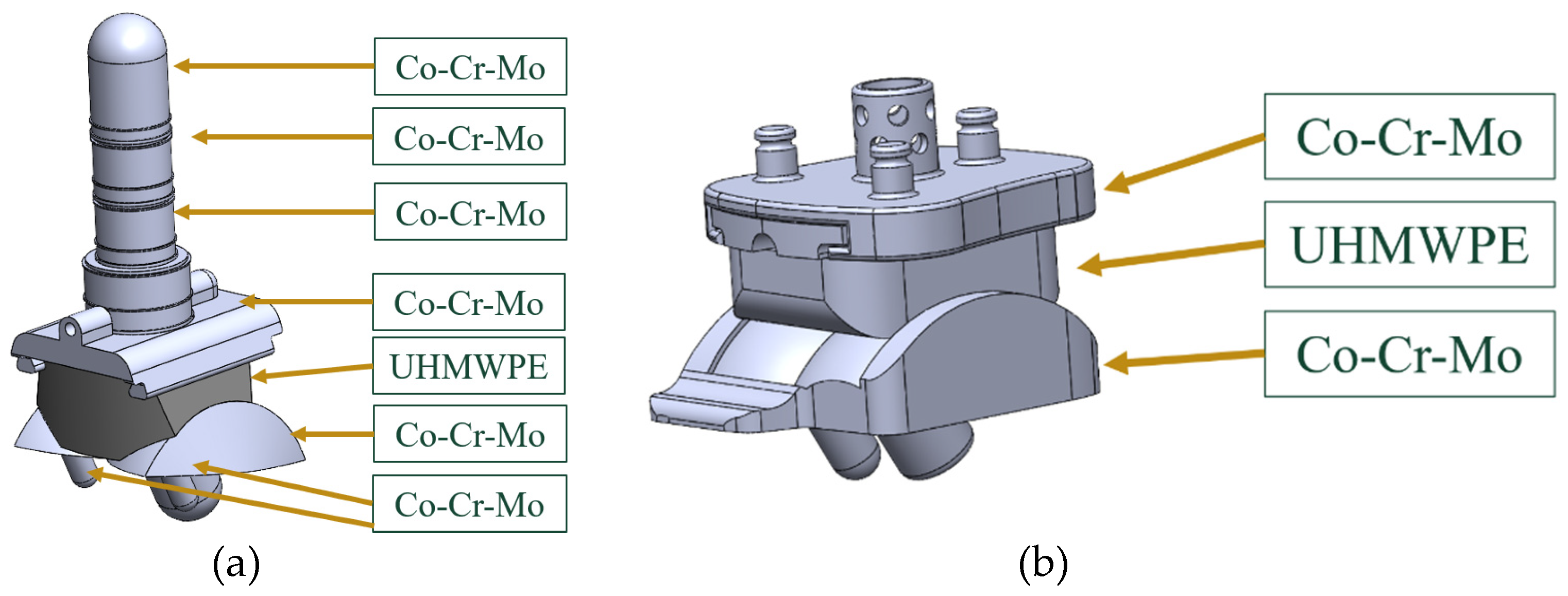
Figure 15.
UHMWPE GUR 1020 True Stress vs. True Strain curve.
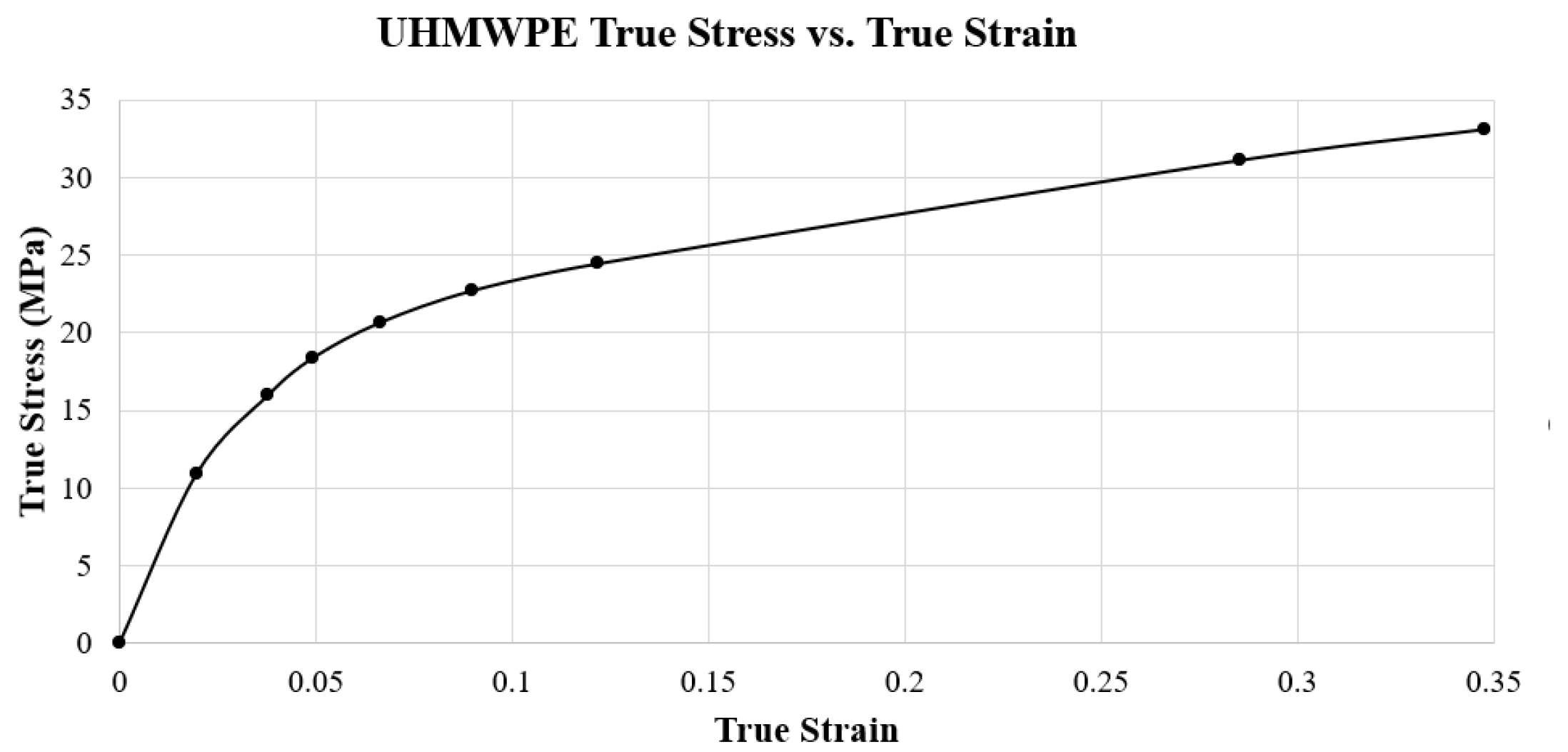
Figure 16.
Visualization of tie constraint between tibial tray and bearing for Vantage.
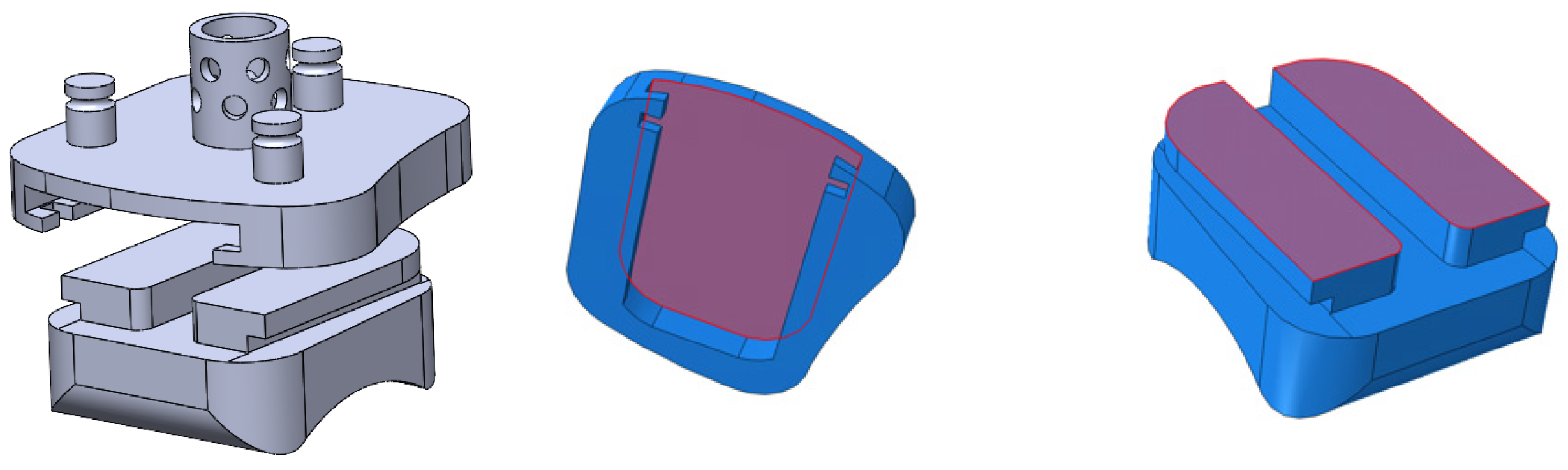
Figure 17.
Dorsiflexion/plantarflexion curve of INBONE II patient [19] with (a) subphases of stance indicated and (b) rotated CAD implant models. Maximum DF angle of 32° at 49% ga.it
Figure 17.
Dorsiflexion/plantarflexion curve of INBONE II patient [19] with (a) subphases of stance indicated and (b) rotated CAD implant models. Maximum DF angle of 32° at 49% ga.it
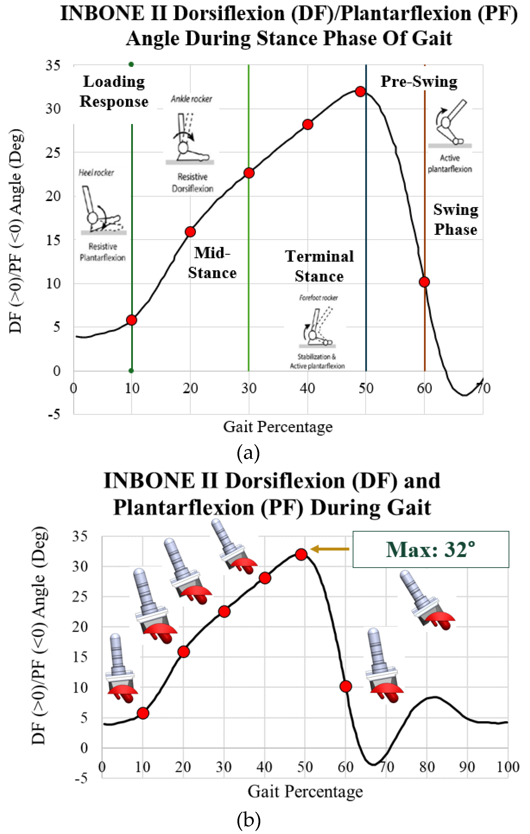
Figure 18.
Axial compressive load on INBONE II patient during gait [19].
Figure 18.
Axial compressive load on INBONE II patient during gait [19].
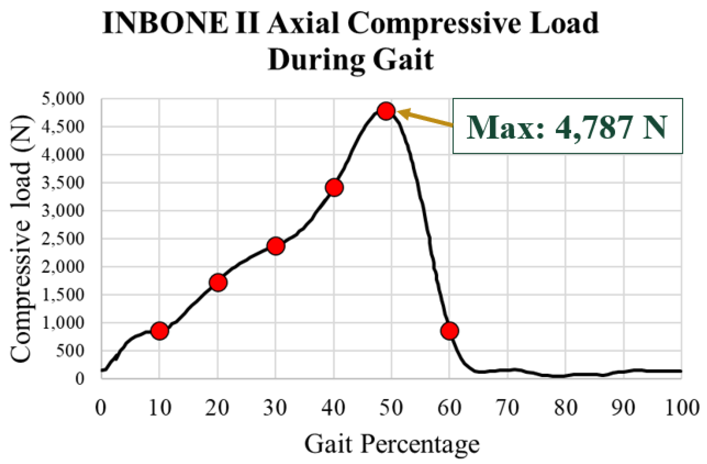
Figure 19.
Loading distribution on INBONE II tibial component with the (a) resultant force and (b) distributed load on stem and tray surfaces.
Figure 19.
Loading distribution on INBONE II tibial component with the (a) resultant force and (b) distributed load on stem and tray surfaces.
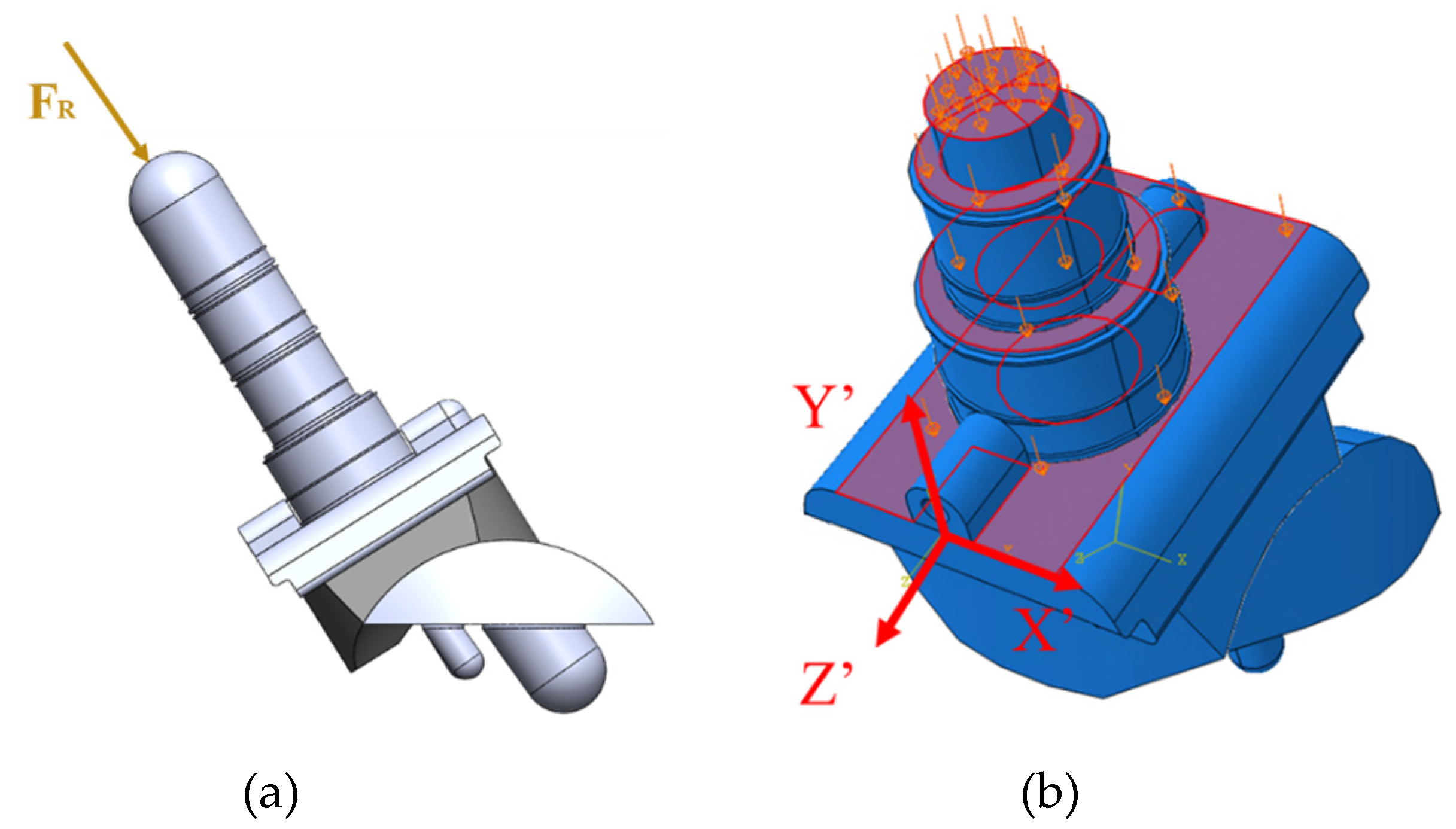
Figure 20.
Dorsiflexion/plantarflexion curve of healthy patient used for Vantage [21]. (a) Subphases of stance and (b) rotated CAD models indicated on pl.ot
Figure 20.
Dorsiflexion/plantarflexion curve of healthy patient used for Vantage [21]. (a) Subphases of stance and (b) rotated CAD models indicated on pl.ot
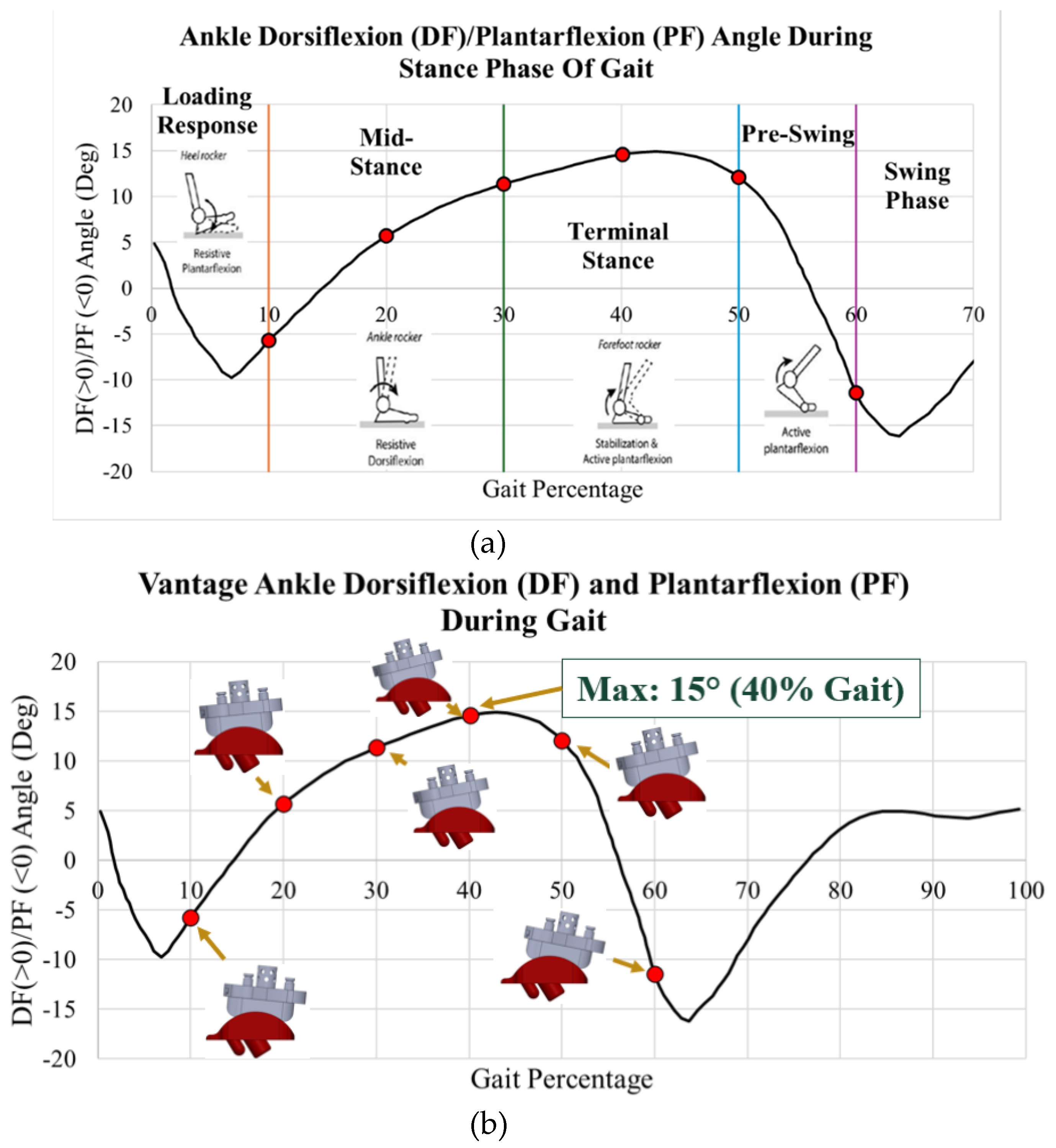
Figure 21.
Axial compressive load on ankle during gait used for Vantage [21]. Maximum load of 3,158 N (40% gai.t)
Figure 21.
Axial compressive load on ankle during gait used for Vantage [21]. Maximum load of 3,158 N (40% gai.t)
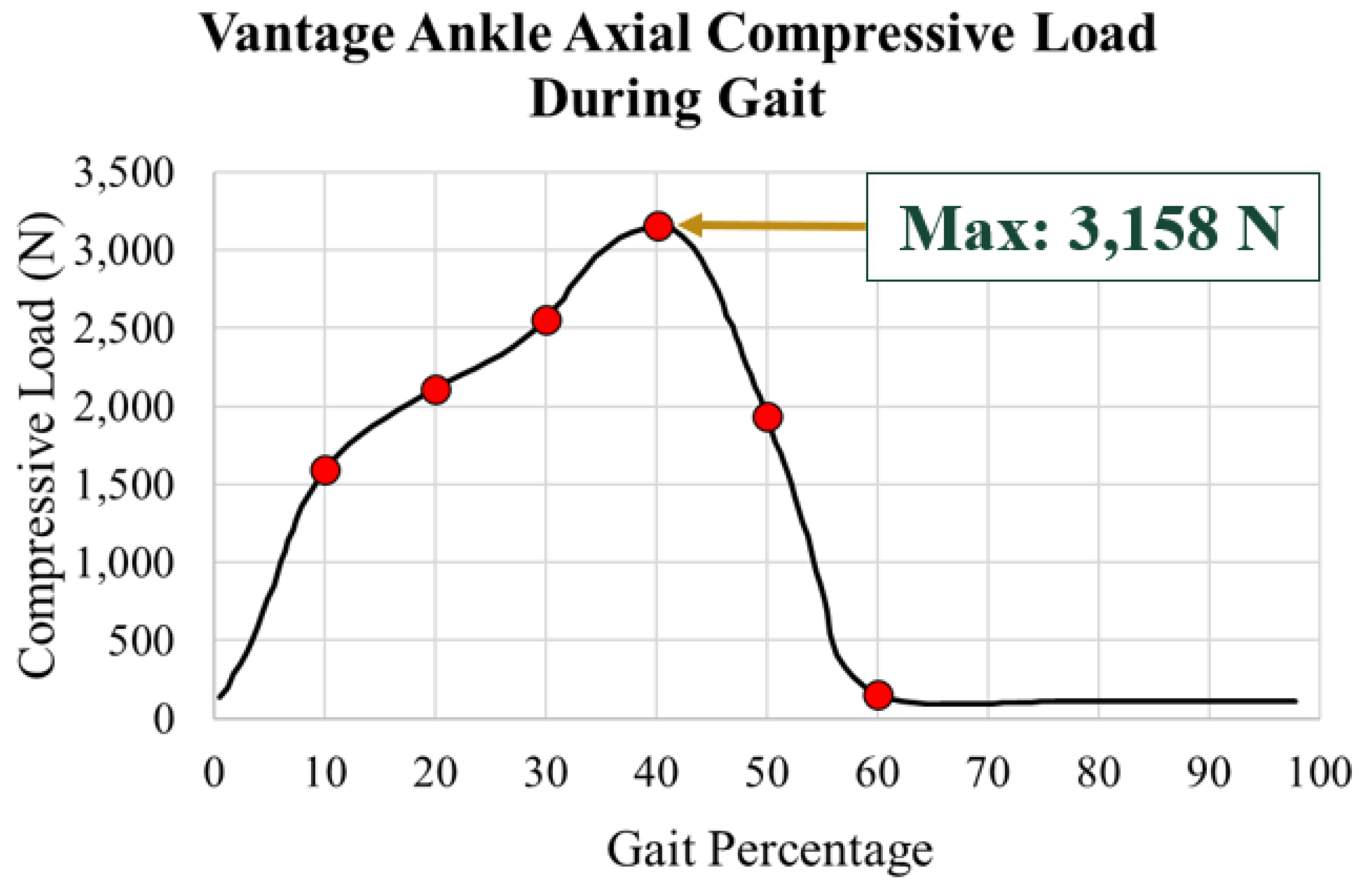
Figure 22.
Loading on Vantage pegs with (a) resultant force and (b) distributed peg loading.
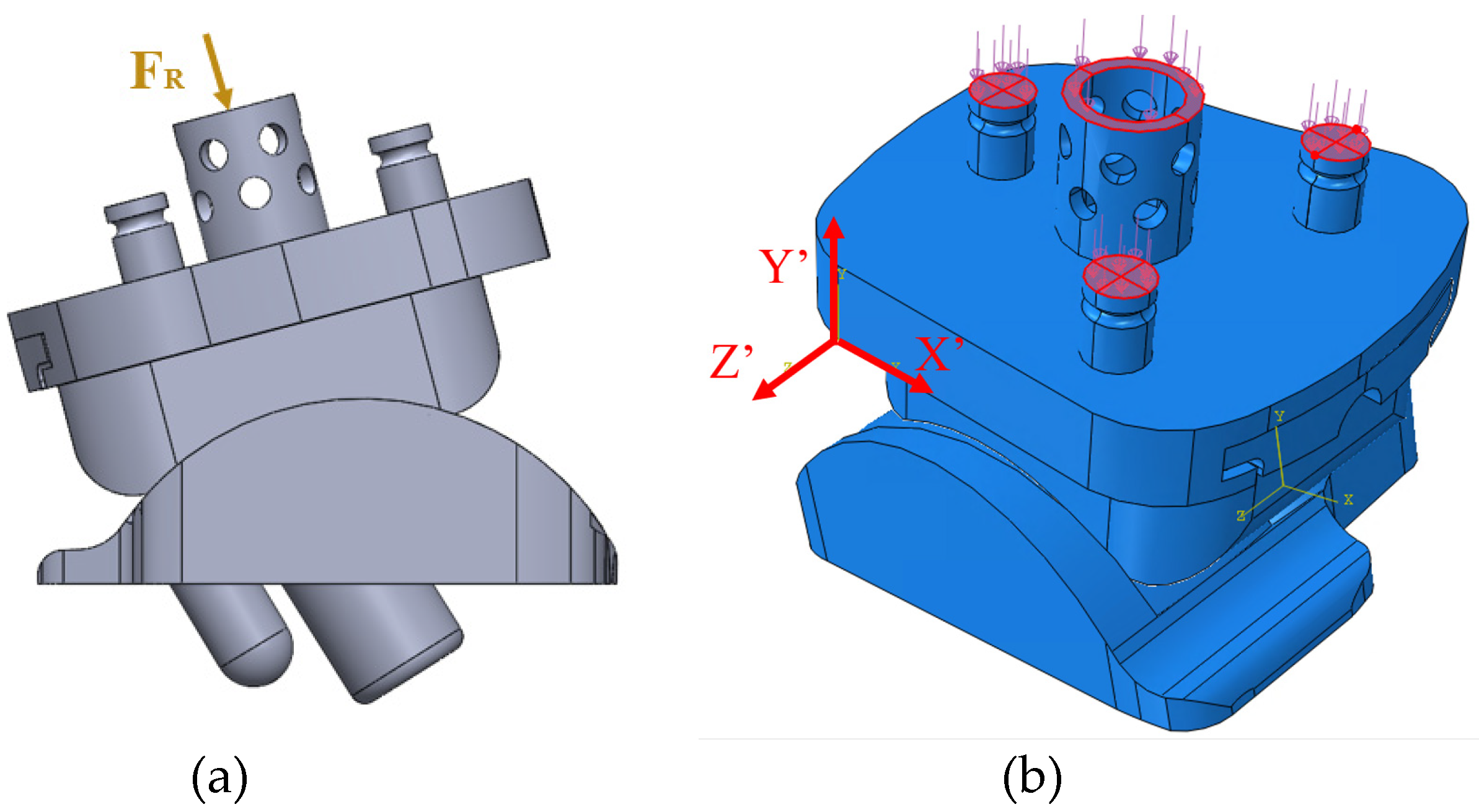
Figure 23.
INBONE II Boundary Conditions with (a) roller constraint on talar face and (b) pin constraint on mid stem center.
Figure 23.
INBONE II Boundary Conditions with (a) roller constraint on talar face and (b) pin constraint on mid stem center.
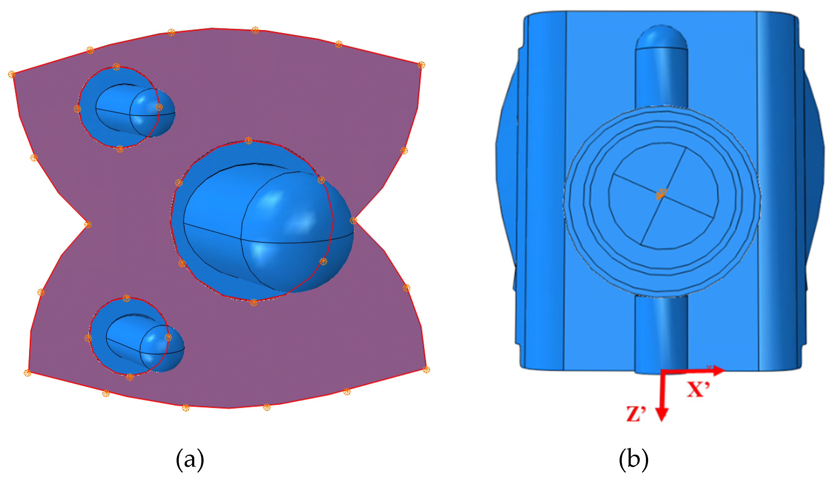
Figure 24.
Vantage Boundary Conditions with (a) roller constraint on talar face, (b) pin constraint on tibial edges, and (c) pin constraint on tibial pegs.
Figure 24.
Vantage Boundary Conditions with (a) roller constraint on talar face, (b) pin constraint on tibial edges, and (c) pin constraint on tibial pegs.
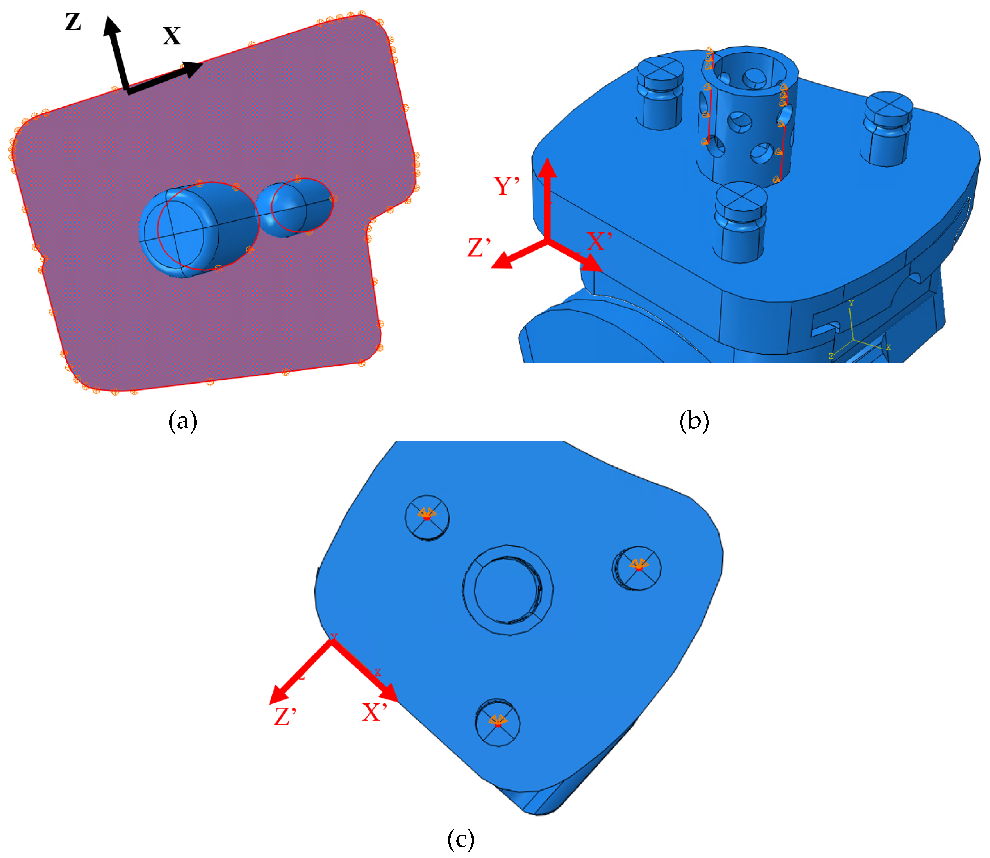
Figure 25.
Summary of mesh convergence for bearing surface of both implants. (a) INBONE II converged at 0.75 mm with 48,102 DOF and the (b) Vantage converged at 0.65 mm with 33,294 DOF.
Figure 25.
Summary of mesh convergence for bearing surface of both implants. (a) INBONE II converged at 0.75 mm with 48,102 DOF and the (b) Vantage converged at 0.65 mm with 33,294 DOF.
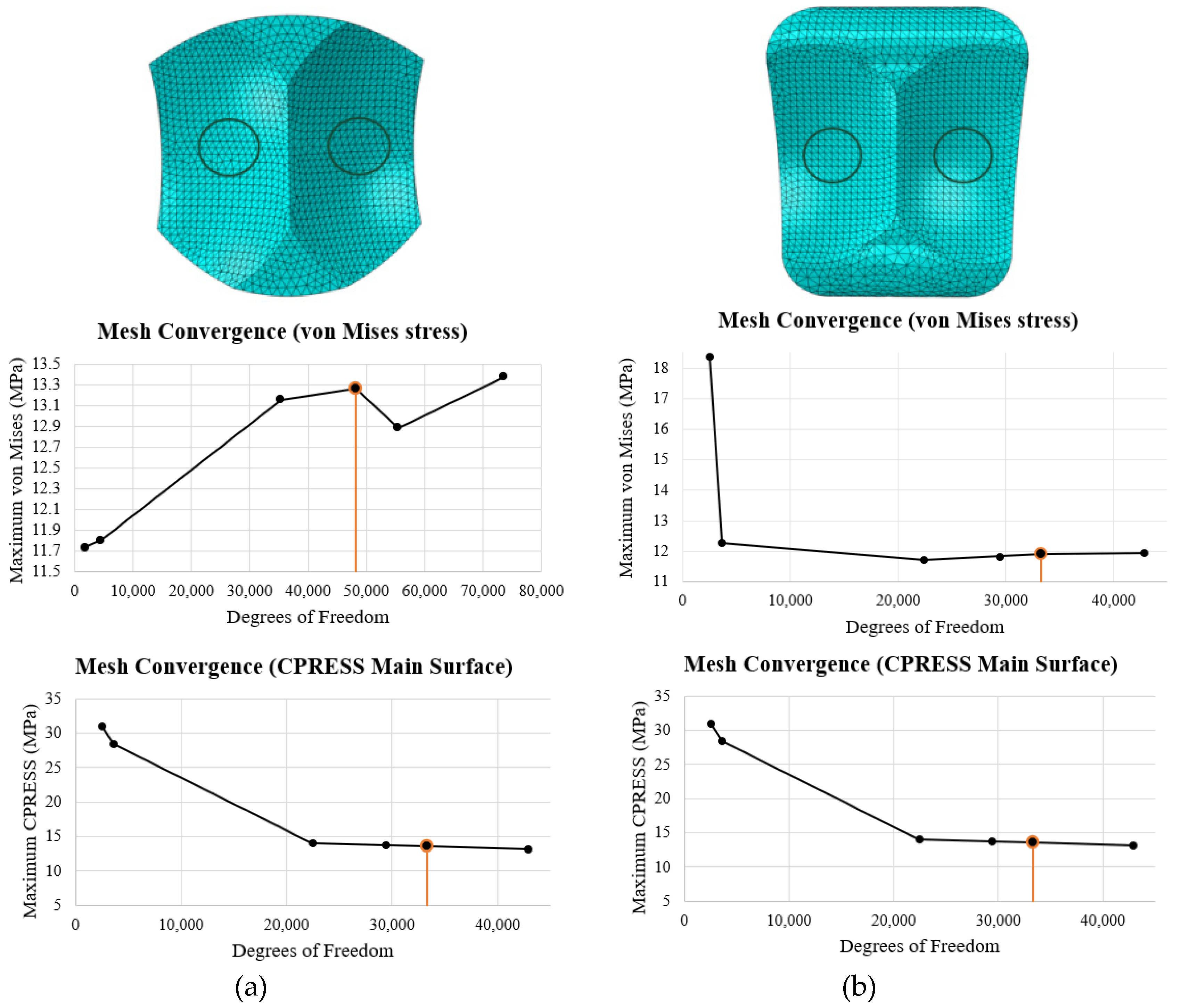
Figure 26.
von Mises stress distributions at maximum loading for both implants.
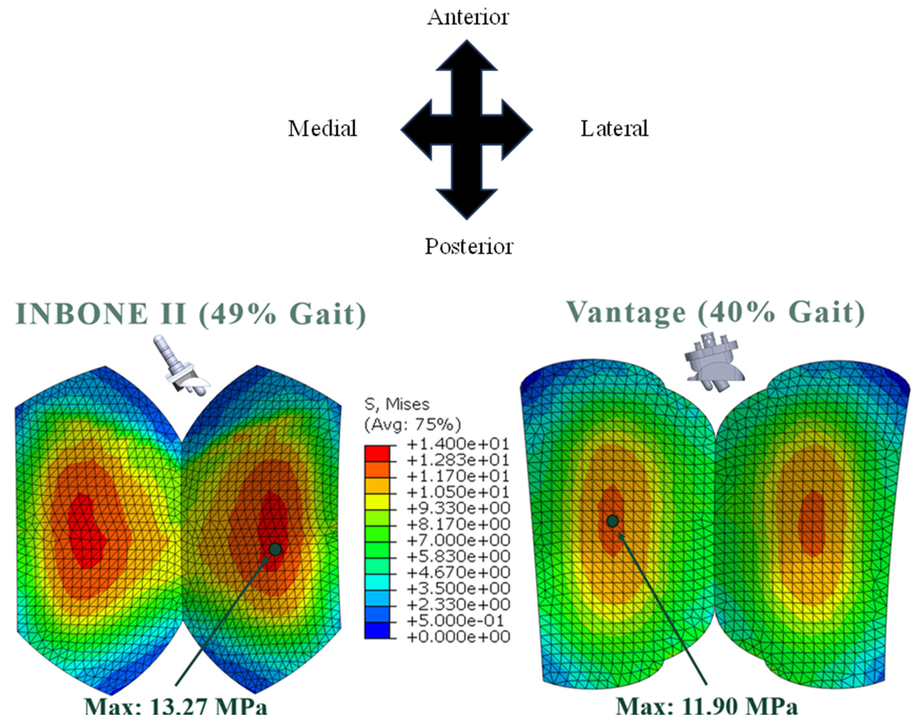
Figure 27.
INBONE II von Mises stress for all configurations with maximum values.
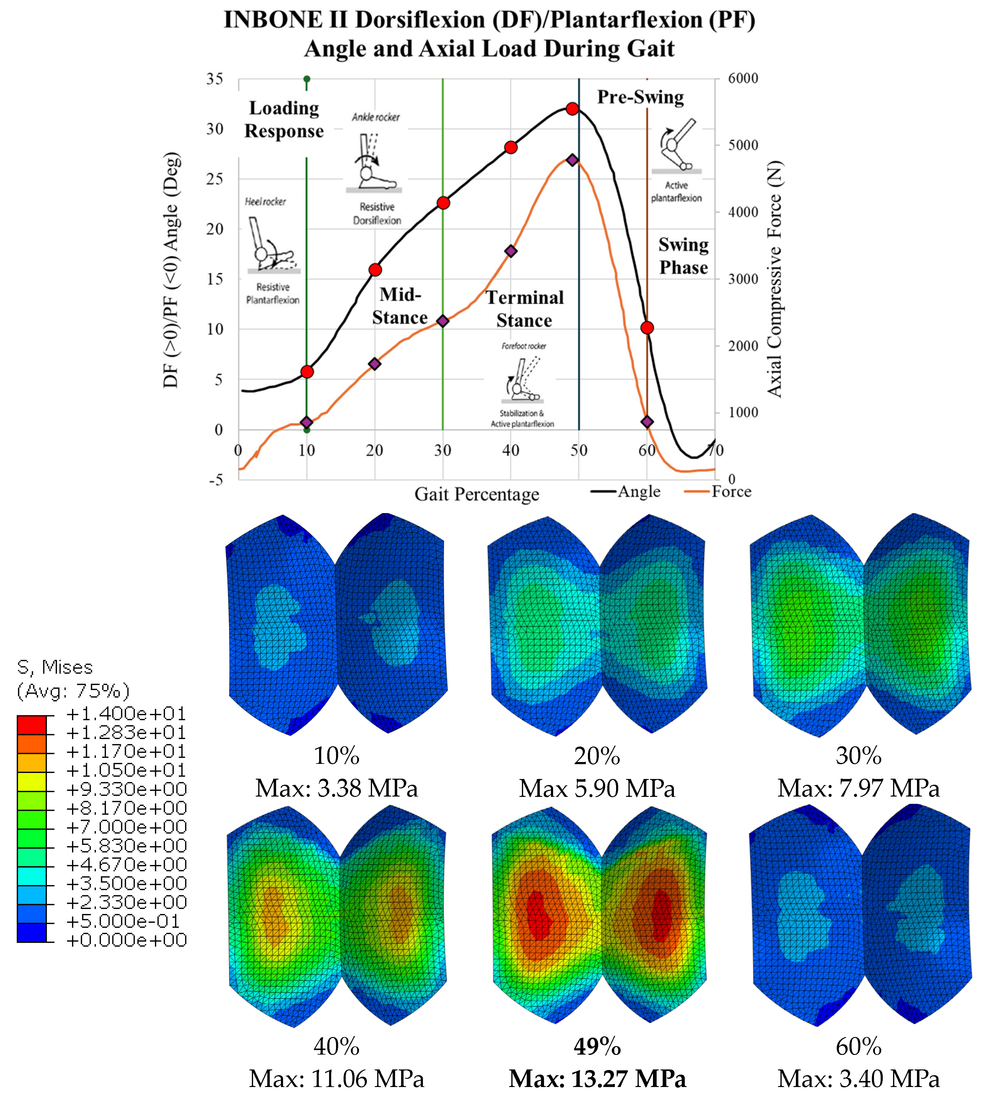
Figure 28.
Vantage von Mises stress for all configurations with maximum values.

Figure 29.
Contact pressure distribution for both implants at maximum loading.
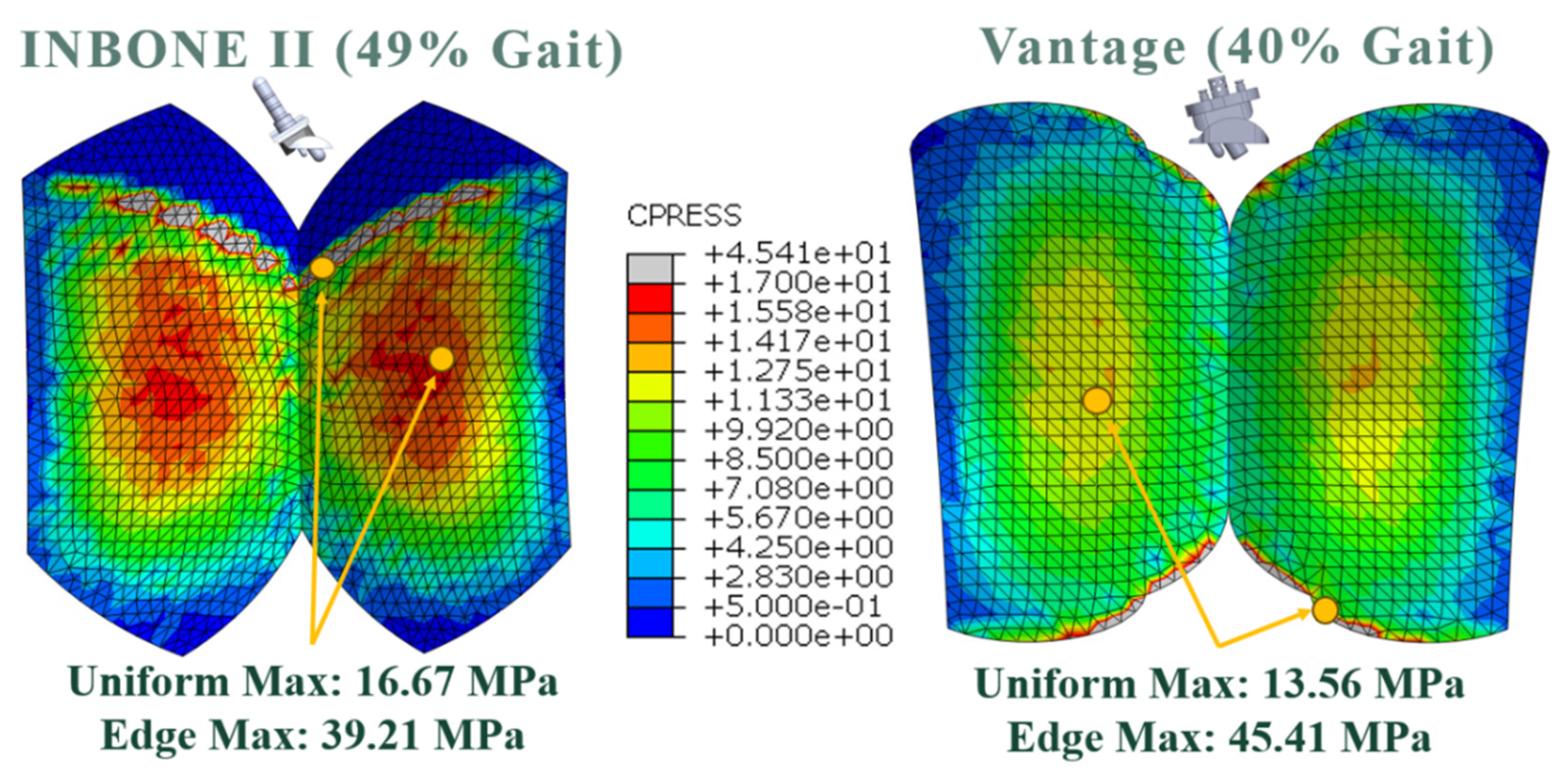
Figure 30.
INBONE II contact pressure distributions for all configurations with maximum values.

Figure 31.
Vantage contact pressure distributions for all configurations with maximum values.
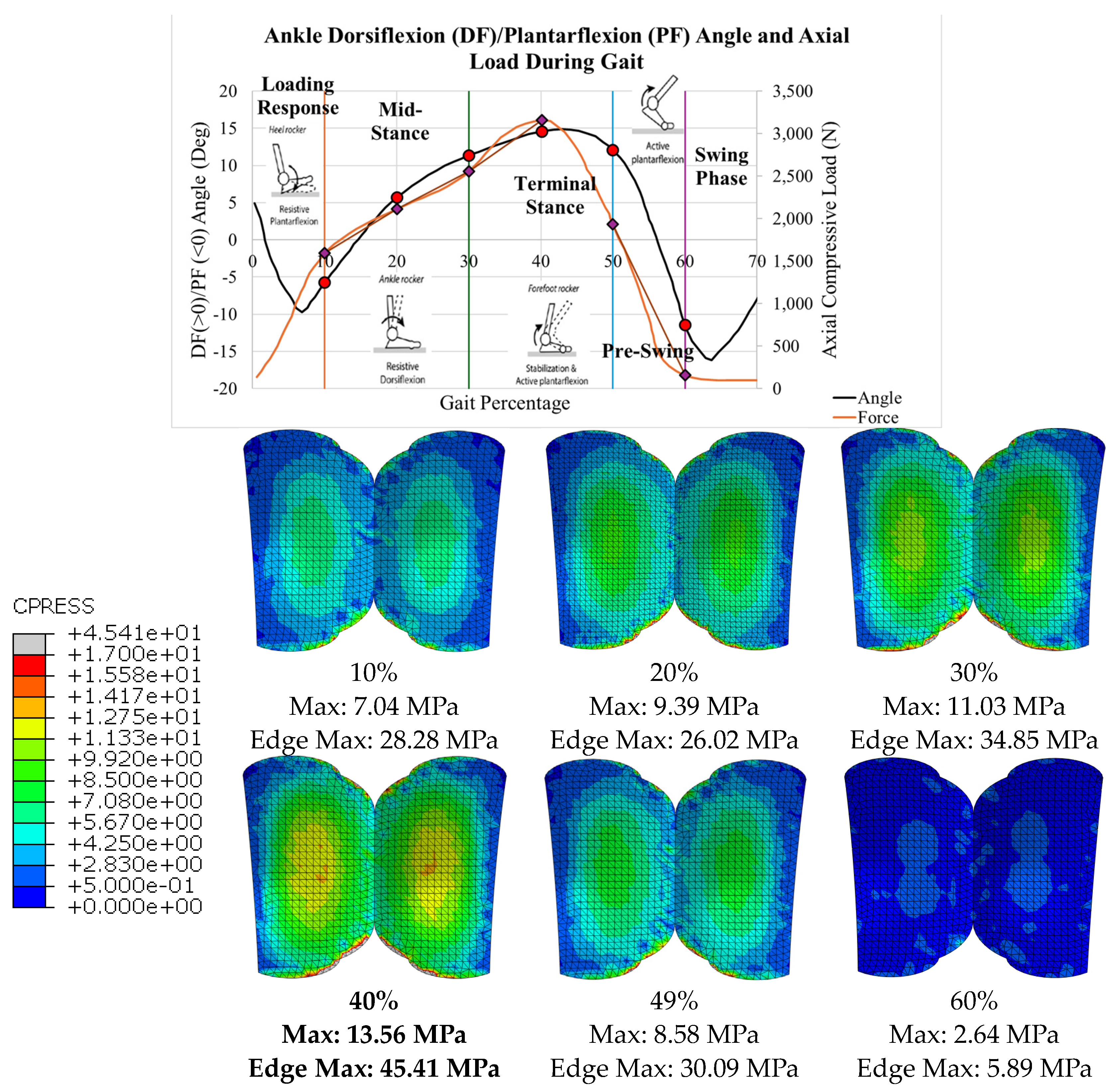
Figure 32.
Stress flow through Vantage bearing on (a) condylar radii, (b) medial radius, and (c) corresponding highest regions of stress.
Figure 32.
Stress flow through Vantage bearing on (a) condylar radii, (b) medial radius, and (c) corresponding highest regions of stress.
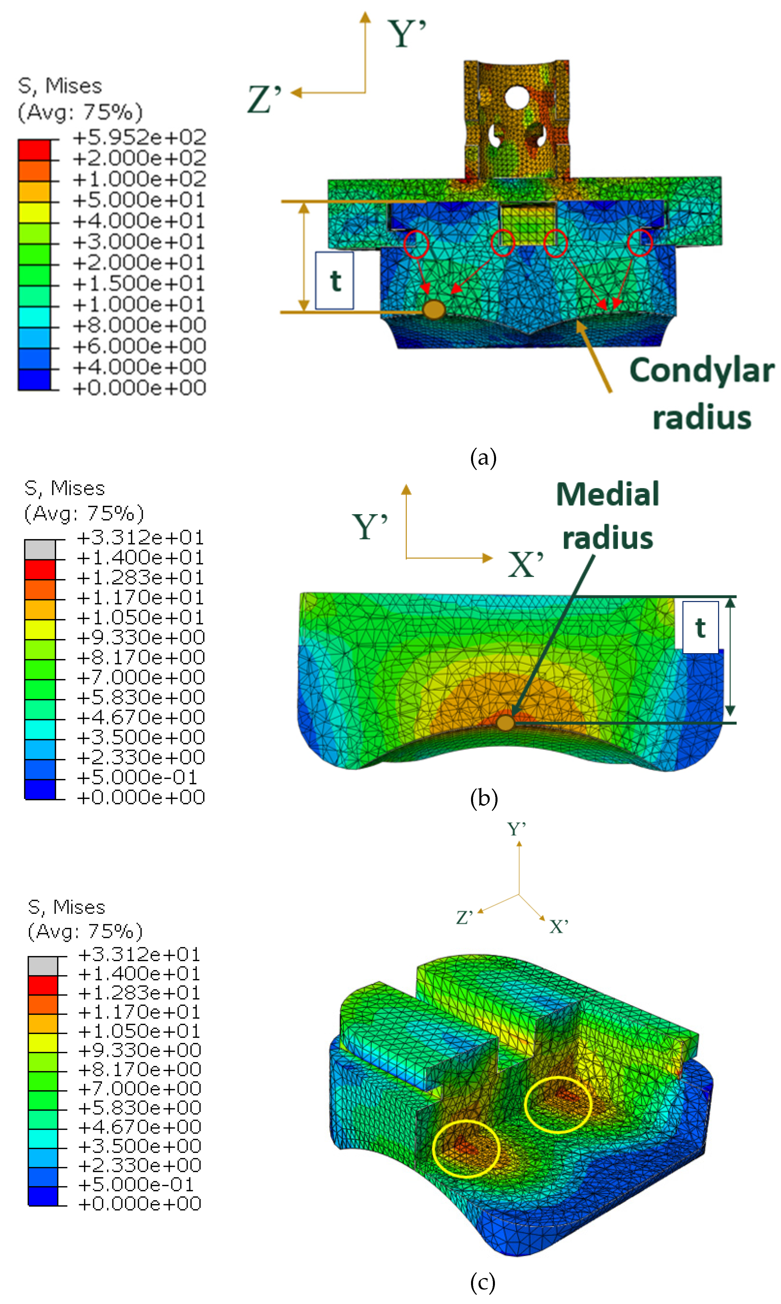
Figure 33.
Effect of (a) unloading (exaggerated for clarity) and (b) re-loading (exaggerated for clarity) on UHMWPE on (c) the yield strength.
Figure 33.
Effect of (a) unloading (exaggerated for clarity) and (b) re-loading (exaggerated for clarity) on UHMWPE on (c) the yield strength.
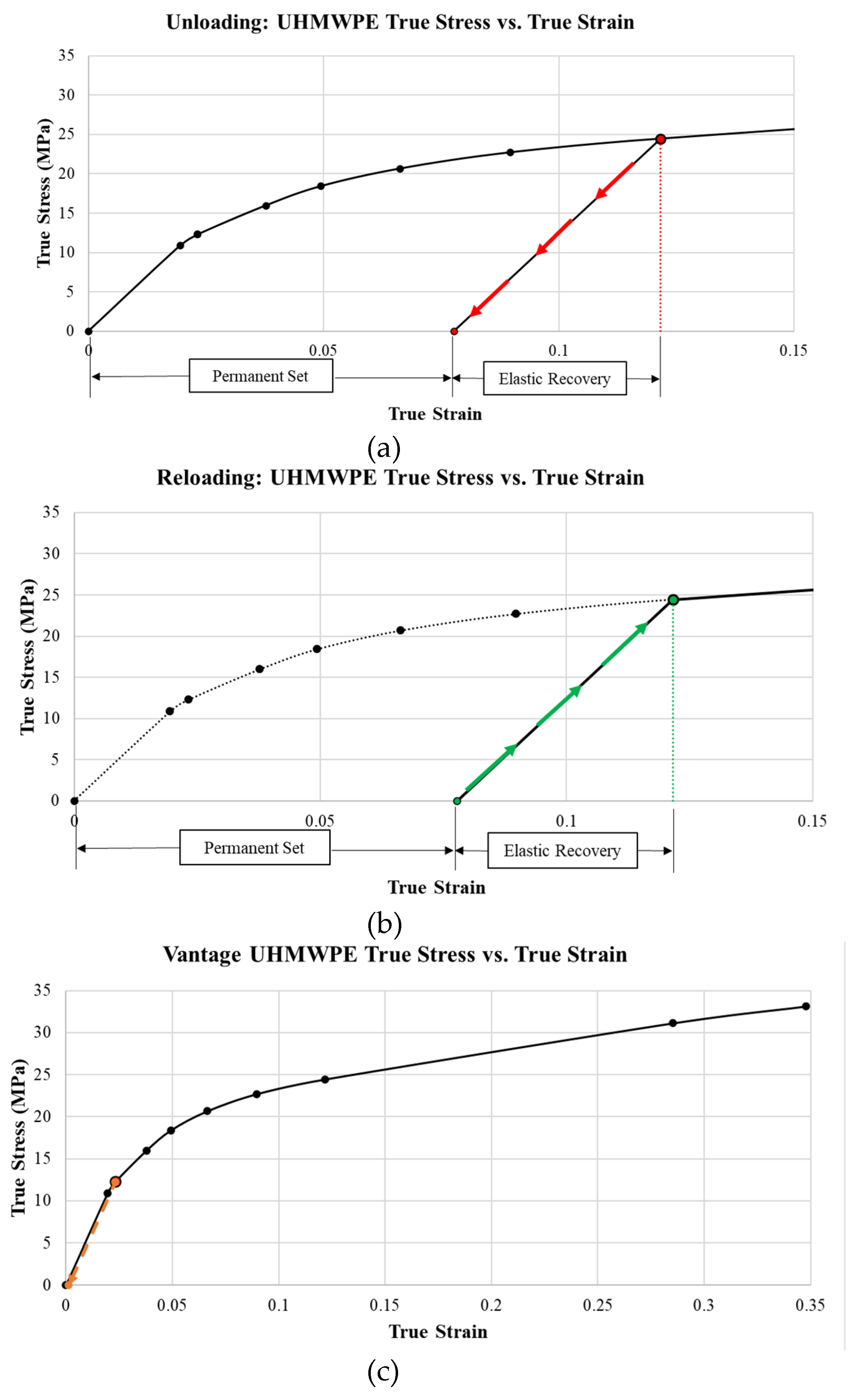

Table 1.
Elastic behavior for materials settings on implants in ABAQUS.
| Material | Poisson’s Ratio | Young’s Modulus (MPa) |
|---|---|---|
| CoCrMo | 0.3 | 210e6* |
| UHMWPE | 0.46 | 557 |
| *Real CoCrMo has E = 210e3 MPa | ||
Table 2.
Summary of Vantage contact settings.
 |
 |
| Main Component | Secondary Component |
| Talar tray | Bearing |
| Normal Behavior | Tangential Behavior |
| Default constraint enforcement“Hard” pressure overclosure | Penalty friction formulationFriction coefficient, µ = 0.04 (Isotropic) |
| Discretization Method | Sliding Formulation |
| Surface to surface | Finite sliding |
Table 3.
INBONE II von Mies stress gait configurations results.
| Gait Pct | Angle | Pressure Load (N/mm2) | von Mises Max (MPa) | Safety Factor (Max) |
|---|---|---|---|---|
| 10 | 5.8 | 1.38 | 3.38 | 3.22 |
| 20 | 16.0 | 2.79 | 5.90 | 1.84 |
| 30 | 22.7 | 3.82 | 7.97 | 1.36 |
| 40 | 28.2 | 5.50 | 11.06 | 0.98 |
| 49 | 32.0 | 7.69 | 13.27 | 0.82 |
| 60 | 10.2 | 1.40 | 3.40 | 3.20 |
Table 4.
Vantage von Mises stress gait configurations results.
| Gait Pct | Angle | Compressive Load N) | von Mises Max (MPa) | Safety Factor (Max) |
|---|---|---|---|---|
| 10.0 | -5.7 | 1,593.95 | 6.75 | 1.61 |
| 20.0 | 5.7 | 2,111.65 | 9.03 | 1.20 |
| 30.0 | 11.4 | 2,555.13 | 10.66 | 1.02 |
| 40.0 | 14.6 | 3,158.26 | 11.90 | 0.91 |
| 50.0 | 12.1 | 1,933.46 | 8.15 | 1.33 |
| 60.0 | -11.5 | 156.28 | 1.44 | 7.56 |
Table 5.
INBONE II contact pressure gait configurations results.
| Gait Pct | Angle | Pressure Load (N/mm2) | CPRESS Max Non-Edge (MPa) | CPRESS Max Edge (MPa) |
|---|---|---|---|---|
| 10 | 5.8 | 1.38 | 5.54 | |
| 20 | 16.0 | 2.79 | 7.73 | |
| 30 | 22.7 | 3.82 | 9.46 | |
| 40 | 28.2 | 5.50 | 12.49 | 22.14 |
| 49 | 32.0 | 7.69 | 16.67 | 39.21 |
| 60 | 10.2 | 1.40 | 5.64 |
Table 6.
Vantage contact pressure gait configurations results.
| Gait Pct | Angle | Compressive Load (N) | CPRESS Max Non-Edge (MPa) | CPRESS Max Edge (MPa) |
|---|---|---|---|---|
| 10.0 | -5.7 | 1,593.95 | 7.04 | 28.28 |
| 20.0 | 5.7 | 2,111.65 | 9.39 | 26.02 |
| 30.0 | 11.4 | 2,555.13 | 11.03 | 34.85 |
| 40.0 | 14.6 | 3,158.26 | 13.56 | 45.41 |
| 50.0 | 12.1 | 1,933.46 | 8.58 | 30.09 |
| 60.0 | 11.5 | 156.28 | 2.64 | 5.89 |
Disclaimer/Publisher’s Note: The statements, opinions and data contained in all publications are solely those of the individual author(s) and contributor(s) and not of MDPI and/or the editor(s). MDPI and/or the editor(s) disclaim responsibility for any injury to people or property resulting from any ideas, methods, instructions or products referred to in the content. |
© 2024 by the authors. Licensee MDPI, Basel, Switzerland. This article is an open access article distributed under the terms and conditions of the Creative Commons Attribution (CC BY) license (http://creativecommons.org/licenses/by/4.0/).
Copyright: This open access article is published under a Creative Commons CC BY 4.0 license, which permit the free download, distribution, and reuse, provided that the author and preprint are cited in any reuse.


