
Submitted:
22 April 2024
Posted:
23 April 2024
You are already at the latest version
Abstract
We present contrast information, a novel application of some specific cases of relative entropy measures, designed to be useful for cognitive modelling of sequential perception of continuous signals. We explain the relevance of entropy in cognitive modelling of music and language. Then, as a first step to demonstrating the utility of constrast information for that purpose, we show empirically that its discrete case correlates well with existing successful cognitive models in the literature. We explain some interesting properties of constrast information. Finally we propose future work towards a cognitive architecture that uses it.
Keywords:
contrast information dynamics
; cognitive modelling
1. Introduction
Information dynamics studies how the information provided by a process changes from one moment to the next. It is concerned with the information provided by specific observations at specific moments in time. Whereas information theory [1] is concerned primarily with the expected behaviour of collections of random variables, information dynamics focuses on specific instantiations of stochastic processes. Both the sequentiality and the specificity of an instantiation of a stochastic process are central to the study of information dynamics. This focus on specific sequences distinguishes information dynamics from information theory more generally.
An instantiation of a stochastic process is a sequence of observations. Designating a point in the sequence as the current moment in time, the sequence can be partitioned into three temporal regimes: the past (previous observations), present (current observation), and future (subsequent observations). Information dynamics measures how these three regimes inform one another. For instance, how much information does the present observation provide about the future given what was seen in the past? This extends beyond stochastic processes that have a natural temporal aspect. For example, the process of estimating model parameters from data can be considered as a stochastic process when that estimation proceeds in a sequence of steps as more data observed. Even when the data are independently and identically distributed, when the data is consumed in sequence in the process of estimation, the result is a stochastic process of the estimated parameter.
Previous work on information dynamics [2,3,4,5] focused exclusively on discrete-time processes with a finite number of discrete states (DTDS process). In order to quantify the information dynamics of a DTDS process, information content and Shannon entropy [6] were used to measure the unexpectedness and uncertainty of a given observation in the context of previous observations. However, when working with stochastic processes of continuous state, neither information content nor Shannon entropy (nor differential entropy) are suited to the task. All three of these measures lack the property of coordinate invariance, also called parameterization invariance. Their value is dependent on the coordinate system used to describe the process. However, relative entropy (KL divergence) is coordinate invariant. In this paper, we specify a form of relative entropy called contrast information that is not only coordinate invariant, but like other common information measures, is also non-negative. Contrast information is closely related to information content and Shannon entropy in the discrete case, but can also be applied to stochastic processes over continuous state spaces.
A discrete-time process can often be considered as a uniformly sampled version of a continuous-time process. However, more generally, observations of a continuous-time process are not required to be uniformly sampled in time. The observations may be spread heterogeneously over an interval, or may be observed continuously, and therefore cannot be treated as simply a discrete-time process. Previous work in information dynamics focused on DTDS processes, always measuring the information provided by the current observation in the context of the immediate past. Something similar is still possible with continuous-time processes, but we must be careful when defining what is meant by the past context, since those observations may be heterogeneously distributed in time or continuously observed.
Contrast information is defined with respect to the three temporal regimes: the past, present, and future. Permuting these temporal regimes in contrast information results in six temporal variants that have different semantics. Predictive contrast information is the amount of information the present provides about the future given the past. Connective contrast information is the amount of information the past provides about the future given the present. Reflective contrast information is the amount of information the future provides about the present given the past. These three forward variants are mirrored by three backward variants.
In the current article, we define contrast information, and show that it has promise as a continuous successor of the former discrete measures already successfully used in cognitive modelling. The structure of this article is as follows. We begin with our theoretical framework for cognitive modelling, the Information Dynamics of Thinking, summarising previous research and explaining why it needs to be extended into continuous state spaces. Next, we lay out the detail of contrast information, and demonstrate how it can be applied to discrete-time and continuous-time Markov and Gaussian processes. We then perform an empirical comparison between the discrete form of contrast information and show that it correlates well with the measures used in earlier work, and thus would produce the same results if used in those models. Finally, we summarise the results and propose future directions for research.
2. Theoretical Framework
2.1. Motivation: Cognitive Modelling
The motivation of the current work arises from a thread of research on computational cognitive modelling of sequential perception, mostly of music. Cognitive modelling as a research field lies at the intersection of psychology and artificial intelligence. Computational cognitive models use computational methods to simulate hypothetical models of human or animal cognitive behaviour, so that the hypothesis can be tested, by comparing the outputs of the simulation with empirical studies of the relevant organism. These comparisons can be made behaviourally, by observing human or animal response, or more objectively by measuring physiological responses, as, for example, in electroencephalography. The benefit of this approach is that it renders very precise and operational hypotheses testable, where they are often difficult or even impossible to test otherwise, often for ethical reasons.
The overarching aim of the work reported here is to underpin a new cognitive model, in which we attempt to generalise a well-established discrete-symbolic statistical model of learning and cognitive prediction to a continuous simulation, which we believe will have greater explanatory power. The ultimate aim is to simulate the working of the mind/brain1 at a level of abstraction rather higher than the neural substrate (wetware), but also much more granular than what is readily achievable by observation alone. The purpose of the current section is to explain enough of this background to render the motivation of the subsequent research report clear, and to provide further references for the interested reader.
2.2. Predictive Cognition
Over the past decade, there has been a flurry of interest in the idea of predictive cognition, which proposes that one key function of cognition is to predict events in the immediate environment of the organism in order to facilitate efficitent and effective actions in that environment. Friston [7] proposes the idea of free energy, equating roughly to entropy, which an organism attempts to minimise by means of prediction from an internal model of the world and correction when the predictions of the model are found to be incorrect. Schmidhuber [8] proposes a model of creativity based on the compression of perceptual data and prediction from the compressed model. Clark [9] convincingly presents the philosophical case for this kind of model.
2.3. The Information Dynamics of Music and Language
Music is an excellent means by which to study the human mind [§3] [10], in particular because it may be considered as a(n almost) closed system [11], requiring very little reference outside itself, and, at the same time, demonstrating cognitive effects rather clearly. It is also worthy of study in its own right, because it is hugely important to humans in general, and is (therefore) also an important economic driver in the modern world.
In the computational study of music, the idea of predictive cognition arose rather earlier than in the work cited above, since music perception and appreciation depend heavily on expectation and the fulfilment or denial thereof [12]. Here, information theory appears in two capacities. First, as in the work of Friston [7], it serves to measure how well a learned model fits the data, overall, from which it was learned. Second, in a more granular application, it serves to measure the local information content and entropy [6] for each tone in a musical sequence. The groundwork for this approach was laid by Conklin [13] (see also Conklin and Witten [14]), by providing a straightforward (though not simple) learning mechanism that could cope with the extreme multidimensionality of musical signals. Pearce [2,15] demonstrated that Conklin’s theoretical model is in fact a cognitive model, by implementing it in what has come to be known as IDyOM, short for “Information Dynamics of Music”, and showing that the predictions of the model correlate well () with human responses, over multiple studies and musical genres. At the time of writing, IDyOM remains the best model of melodic pitch perception in the music cognition literature.
IDyOM models human cognition using discrete symbols for pitch and musical time. Each musical tone is represented as a tuple of musical features, each of which contributes to a variable-order Markov model, as specified by Conklin and Witten [14] and Pearce [2]. Using the Prediction by Partial Match (PPM) algorithms [16,17] a distribution is obtained for each feature at each point in a melody. These distributions are then combined in an empirically validated model [18] to produce one distribution over musical pitch (again represented discretely). This distribution is shown to correlate well with empirical data from earlier and new studies of musical expectation [19,20]. Furthermore, the information-theoretic outputs of the system, in terms of information content of observed symbols and entropy of the distributions from which they are drawn [6] have been shown to correlate with human perception at what might be called a meta-level with respect to pitch prediction: information content correlates with unexpectedness of what is perceived[20], and entropy correlates with uncertainty experienced during perception [21].
In a prequel to Schmidhuber’s model [8], Pearce [2] and Pearce and Wiggins [22] showed how prediction from statistical models can simulate the creation of novel music. This work underlines the need for simulations that can learn the representations that they use, a property that symbolic systems usually lack, and on which the current success of deep learning depends.
2.4. Sequence Segmentation and Boundary Entropy
The information-theoretic outputs of IDyOM can also be used to analyse structure in music, using the detection of boundary entropy [23,24]. The idea here is that, if a sequence of data exhibits sequential regularity of the kind naturally captured by a grammar, then both information content entropy will trend downwards on average from the start of a structural unit towards its end, because the available context within the structural unit is supplying progressively more information. After the end, there will be an increase in entropy because the statistical correlation across the boundaries between structural units is weaker than that within them, and so less contextual information is available. This principle has been shown to allow structural boundaries to be identified in melodies of various kinds [23], by means of a simple process of peak picking in the information-theoretic signal: a large peak in the current context tends to coincide with the first symbol in a new structural unit. Sequence processing, as a human capacity, is of course more general than music and IDyOM has also been used to determine the segmentation of English language, on one level [25], and hierarchically [26]. The idea of boundary entropy finds support in results (in both music and other sequences) suggesting that the chunks so formed are stored as separate units, thus making them available for subsequent predictions [27,28]. Based on this, Wiggins and Sanjekdar [29] applied the same idea to text, successfully identifying morpheme and word boundaries, while also proposing an entropy-based simulation of memory consolidation that guides model correction by identifying high information content in the stored model.
In related research, Abdallah and Plumbley [4] considered a broader range of information-theoretic simulations, successfully applying them to a range of artificial musical data. Pearce and Wiggins [3] and Agres et al. [5] present summaries of the work applied to music.
In summary, there is substantial evidence that human experience of information quantities, as simulated by Shannon measures [30], play a direct part in the working of the non-conscious and the conscious mind/brain. In other words, it seems that humans are both consciously and non-consciously sensitive not just to the content of perceptual signals, but also to their information-theoretic properties.
2.5. The Information Dynamics of Thinking
The discrete symbolic simulations described above constitute good evidence that information dynamics offers a route to understanding some important aspects of human cognition. Wiggins [10] proposes to generalise these ideas beyond musical stimuli (while still maintaining music as a paramount way in to human cognition), and, crucially, to a continuous world model. This proposal views the mind/brain as a collection of interacting oscillatory systems, a view which is increasingly gaining traction in cognitive science (e.g., [31,32]). In this proposal, perceptual signals are represented as waves, and therefore sound is a particularly good starting point: recent research shows that perceived sound and its significant correlates are reproduced as electrical waves in the mind/brain, notwithstanding the fact that it has been deconstructed by the ear prior to its arrival in the auditory cortex [33,34,35].
The Information Dynamics of Thinking (IDyOT) cognitive architecture [24] proposes a cyclic process of learning and segmentation to build a model of continuous percepts that is analogous to the discrete models of IDyOM. A process of categorisation based on structural similarity of segments allows the same process to be applied repeatedly, building layers of progressively more abstract and less granular representations, as in the work of Wiggins and Sanjekdar [29]. (This process is similar to the process of deep learning of representations, the methodological benefit being that the IDyOT model is driven, bottom up, by scientific theory. In contrast, information loss in the training of deep networks generally renders their operation inscrutable and therefore generally not amenable to scientific enquiry as cognitive models. This issue has spawned the new research subfield of explainable artificial intelligence.)
Homer et al. [36] show how the lowest layer of an IDyOT model of Western Tonal Music might be based in a Hilbert Space of Resonances, directly representing cognitive representations of musical sound. However, this work does not encompass the need for segmentation, because it focuses on static representations of static percepts. The current article presents a novel method to underpin segmentation in a time-variant version of this and other representational spaces of the same mathematical kind. In the following sections, we introduce a set of information-theoretic measures that admit the analysis of information dynamics in continuous representations, in a way analogous to information content and entropy in the discrete case outlined above. Given such measures, the way is open to determining boundary entropy and an implementation of segmentation in IDyOT. To ensure that the measures remain consistent across the divide between discrete and continuous representation, we demonstrate a good correlation between the former measures and our new measures applied in the discrete case.
3. Information Dynamics in Continuous Systems
3.1. Motivation and Structure of the Article
The overarching contribution of the current paper is to propose and validate a set of novel information measures that extend the theory of Information Dynamics beyond discrete representations to continuous ones.
First, we introduce and motivate the new measures in detail, discussing useful mathematical properties in relation to the discrete models outlined above. We discuss the behaviour of the models in context of standardised distributions. Then, using our new implementation of discrete models, IDyOMS, we show a good correlation between the earlier discrete information measures and the new continuous ones applied in the case of discrete data, as applied to music data. Therefore, we are confident that a model of segmentation based on the new continuous model will perform similarly to the existing successful discrete model. Finally, we summarise the contribution of the paper and describe opportunities for future work.
3.2. Coordinate Invariance
The principle of coordinate invariance [37], also called parameterization invariance or general covariance, states that Nature does not possess a coordinate system; all coordinate systems are imposed by us to aid in our analysis of Nature. As such, the fundamental quantities of Nature must be invariant to the coordinate system used to describe those quantities, since they exist outside our means to describe them.
For instance, suppose we are measuring the outside temperature each morning. Generally, temperatures do not generally vary wildly from day to day, so observing today’s temperature gives you some information about what tomorrow’s temperature may be. The temperature itself does not change depending on whether you measure in Fahrenheit or Celsius, so the amount of information provided by those observations must be the same whether you described those temperatures in Fahrenheit or Celsius. Those are just two different coordinate systems describing the same sequence of observations. In the same way that the temperature itself remains the same regardless of whether you describe it in Fahrenheit or Celsius, the information provided by those temperatures should remain the same as well. It cannot depend on the coordinate system used to describe the process. Therefore, a measure of information should be coordinate invariant because the information provided by an observation is independent of the coordinate system used to describe that observation.
Note that describing a quantity in a different coordinate system is different from describing a quantity at a different level of granularity. To continue with the example, we could describe the temperature as hot, pleasant, brisk, cold, or freezing, instead of referring to Fahrenheit or Celsius. The information provided by these categories of temperatures is different from the information provided by the reading in Fahrenheit or Celsius. They are a whole different level of granularity, not a different coordinate system, and so are not subject to coordinate invariance.
Though there is a larger class of coordinate transformations that can be applied in the discrete case, since we are concerned with the information dynamics of continuous state spaces, we will focus on differentiable coordinate transformations.
Definition 1
(Coordinate Transformation). A coordinate transformation, is a differentiable, invertible function . That is, for all and , and , and ; i.e., they are both differentiable.
Definition 2
(Coordinate Invariance). A function f is coordinate invariant iff, for all and , and for all coordinate transformations φ and ,
In short, coordinate invariance just means we get the same result regardless of the coordinate system being used. For us, this is particularly relevant for probability distributions. For discrete random variables, a coordinate transformation amounts to relabeling the elements in with the corresponding elements in .
As such, any measure of information involving discrete random variables is automatically invariant to coordinate transformations. In particular, information content and Shannon entropy are coordinate invariant when working in a discrete state space.
However, when working with continuous random variables, the picture looks slightly different. In addition to relabeling the elements of with the corresponding elements of , we must also scale the probability density according to the absolute value of the derivative of the coordinate transformation, evaluated at x.
In higher dimensions with a vector of continuous random variables, we scale according to the determinant of the Jacobian.
A point of clarification. We are concerned with the information provided by a specific observation. In the discrete case, an observation corresponds to an event that we can assign a nonzero probability; however, in the continuous case, the probability of a specific observation is always zero. Nonetheless, we still want to associate some amount of information with that specific continuous-valued observation, not a quantized version of that observation.
3.3. A Continuous Alternative for Information Content
We want a measure of information that works with both discrete and continuous state spaces, but is also coordinate invariant. Since all measures of information are coordinate invariant in the discrete case, we must check if they are coordinate invariant in the continuous case. Previous work relied on information content and Shannon entropy to measure the information dynamics of a sequence. However, information content is not coordinate invariant.
Theorem 1.
When X is continuous, information content x is not coordinate invariant.
Proof.
Given a coordinate transformation for all with X continuous,
Suppose for some constant .
Since generally, , information content is not coordinate invariant. □
Shannon entropy is only defined for discrete state spaces, so it unsuited for continuous state spaces unless the space is first quantized into a discrete state space Quantization ([1] [Ch. 10]) is a different problem than the one addressed in this paper. The continuous analogue of Shannon entropy is differential entropy ([1] [Ch. 8]), however, like information content, differential entropy is not coordinate invariant.
Theorem 2.
When X is continuous, differential entropy is not coordinate invariant.
Proof.
Given a coordinate transformation for all with X continuous, the differential entropy 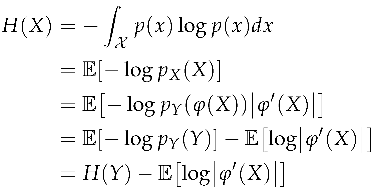
Suppose for some constant .
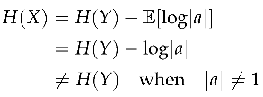
Since generally, , differential entropy is not coordinate invariant. □
Therefore, since information content, Shannon entropy, and differential entropy cannot be used in the continuous case, we must look to other measures of information.
Though closely related to Shannon entropy and differential entropy, mutual information is a measure of information that is coordinate invariant, a property it inherits from relative entropy (KL divergence) [38]. However, mutual information measures the expected information between random variables, To get the amount of information provided by a specific observation, we instead use specific information [39]. Like relative entropy and mutual information, specific information is also coordinate invariant.
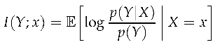
Definition 3
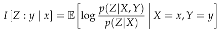
(Specific Information). Specific information I() is the amount of information gained about some unobserved variable Y from observing a specific outcome x.
Theorem 3.
When Y is continuous, specific information is coordinate invariant.
Proof.
Given a coordinate transformation for all with Y continuous, the specific information I()
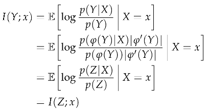
Therefore, specific information is coordinate invariant. □
There are other definitions of specific information. One such alternative definition, response-specific information [40], like information content, has the desirable property of additivity in discrete case; however, it is not coordinate invariant in the continuous case, so we focus on definition of specific information shown here.
4. Contrast Information
4.1. Contrast Information
In the previous section, we examined whether a few common measures of information are coordinate invariant when dealing with continuous random variables, finding that relative entropy, mutual information, and specific information fit the bill. We will now define contrast information in terms of specific information.
Definition 4
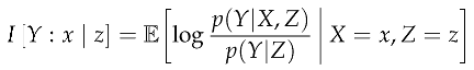
(Contrast Information). Given a stochastic process S and index set T, with convex disjoint subsets giving the target , source , and context , the contrast information is the conditional specific information about a target A from observing a specific source in a specific context .
Depending on whether is a discrete or continuous state space, the expectation in contrast information takes the form of a sum or integral, respectively.


Though contrast information is a particular form of specific information, we will use a slightly different notation to visually distinguish from specific information and mutual information. The square brackets and colon make it clear that we are referring to contrast information in particular, as opposed to the more general specific information. The target A is in the first position to the left of the colon, which is the random variable over which the expectation is taken. The source S is in the second position to the right of the colon, which is a specific outcome given in the conditional expectation. The context C is in the third position to the right of the vertical bar, a specific context also given in the conditional expectation.
Contrast information is a particular form specific information, which is itself a particular form of relative entropy. Since relative entropy, and therefore contrast information, can be thought of as the expected amount of information provided [41] by each sample that aids in discriminating in favor of the distribution from when is the case. If is very similar to , determining that is the case instead of is difficult. You would need to draw many samples to be confident that is the case instead of . Since they look so similar, there is little with which to discriminate between them and therefore a small relative entropy from to . If the distributions look very different, then fewer samples will be necessary in order to discriminate that is the case instead of .
Since these two distributions differ only in the given source , contrast information measures the degree to which that source affects the target given the context. If it is difficult to discriminate from , it means that the source did not affect the distribution of the target, at least relative to the context. Contrast information measures this effect by looking solely at the change in the distribution of the target. Even when we have definitely observed a specific source , if the contrast information is small or zero, it would be difficult to say we observed anything happening at all looking only at the distribution of the target. When contrast information increases, observing a specific source is distinguished from the context, since its presence causes to look very different from .
Target, source, and context. All three regimes are essential components of contrast information. Given the same context, different sources may provide varying amounts of contrast information about the target. Similarly, different contexts given the same source may provide different contrast information about the target. In section: Temporal Variants, we will examine temporal variants of contrast, where the temporal ordering of the target, source, and context regimes determines the semantics of each variant of contrast information.
To provide some intuition about contrast information by way of analogy, suppose you are sitting at a red light at a car intersection. After a little while the light turns green; you hit the gas to pass through the intersection. Prior to the light turning green, each moment observing the red light was much like the previous moment. One moment at the red light followed by another is a rather monotonous situation. But when the light turns green, things change dramatically as you hit the gas to move forward. Sitting at the red light and observing the red source in a red context corresponds to a small or even zero value of contrast information, since distinguishing between different moments at the red light is difficult. Once the red light turns green, contrast information increases, because observing the present source in a red context causes a dramatic shift in your behaviour, changing from a stopped car to driving the car forward.
We can formalize the intuition behind this analogy if we (unrealistically) model the stop light as a two-state Markov chain, where at any moment in time the probability of remaining the same color is much higher than the probability of changing colors.
Example 1.
Suppose we have a two-state Markov chain S with aREDstate andGREENstate. The probability of remaining the same color is and the probability to change colors is .
When the light remains red, the contrast information is nearly zero.
When the light turns from red to green, the contrast information jumps to almost three bits.
4.2. Expected Contrast Information
With respect to the target, contrast information is a function of a specific source and specific context. As such, when the source or context are unknown and represented as random variables, then contrast information is also a random variable. To represent contrast information as a function of a random variable, we write I[] for an unknown source and I[] for an unknown context. The expected value of the contrast information can then be evaluated over either the source, the context, or both the source and context.
When we take the expectation over an unknown context with a fixed source, we arrive at the expected context contrast information.
Definition 5
(Expected Context Contrast Information). Expected context contrast information is the expected value of the contrast information over the context, leaving the source fixed.
When we take the expectation over an unknown source with a fixed context, we arrive at the expected source contrast information, which is equal to the mutual information I() between the source and target given a specific context.
Definition 6
(Expected Source Contrast Information). Expected source contrast information is the expected value of the contrast information over the source, leaving the context fixed.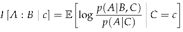
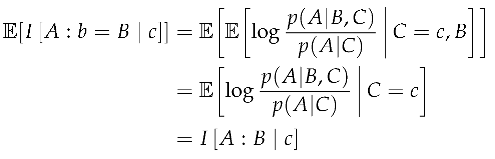
When we take the expectation over both an unknown source and context we arrive at the expected contrast information, which is the same as the conditional mutual information between the target and source given the context.
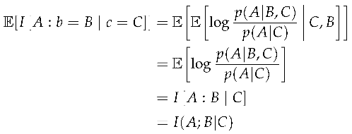
Definition 7
(Expected Contrast Information). Expected contrast information is the expected value of the contrast information over both the source and context.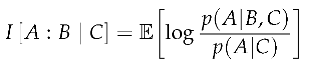
Note the difference in notation between the contrast information of a random variable, like and and the shorthand for expected contrast information over those random variables, such as and . When working with contrast information, if the letter is capitalized, the expectation is taken over that variable. If it is lowercase, then it appears as a given in the conditional expectation.
4.3. Relationship with Information Content
In the previous sections we saw that contrast information is intimately related to specific information and mutual information. In this section, we will see that in the discrete case, contrast information and information content are also closely related.
The property of non-negativity is widely used in information-theoretic inequalities in order to prove bounds on certain quantities. Like information content and other measures of information, contrast information is also non-negative.
Theorem 4.
Contrast information is non-negative.
Proof.
Contrast information is a specific form of relative entropy.
Since relative entropy is always non-negative, so is contrast information. □
In the discrete case, contrast information is not only non-negative, but it has an upper bound of information content, meaning that contrast information is always wedged between zero and the value of information content.
Theorem 5.
In the discrete case, the contrast information is a lower bound on information content .
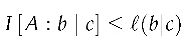
Proof.
Given a stochastic process with discrete, split into target , source , and context ,
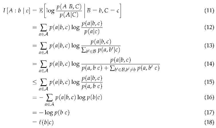
Therefore, . □
If we think of contrast information as estimating information content, then the mean absolute error (MAE) between information content and contrast information is equal to the conditional entropy H(), which is the same as the difference between the entropy H() and mutual information .
Theorem 6.
In the discrete case, the mean absolute error (MAE) between information content and contrast information is equal to the conditional entropy H().
Proof.
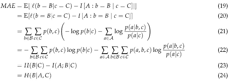 Therefore, the mean absolute error between the information content and contrast information is equal to the entropy H(). □
Therefore, the mean absolute error between the information content and contrast information is equal to the entropy H(). □This implies that the MAE represents the complexity in the source that is not explainable using the target and context. When the source is a function of the target and context, the MAE goes to zero. When the source is independent of the target and context, then the MAE attains its maximum value of B.
Corollary 1.
The mean absolute error (MAE) between information content and contrast information and is a monotonically decreasing function of the length of A and the length of C with a maximum possible value of H(B).
Proof.
The target A and context C can be vectors of random variables. Since conditioning can only maintain or decrease entropy, conditioning on longer vectors of A or C can only maintain or decrease the entropy H(). Therefore, and the MAE is a monotonically decreasing function of the length of A or C with a maximum possible value of B, which is attained when H(B) is independent of A and C. □
5. Temporal Variants of Contrast Information
In order to analyze how information changes in time, it is useful to partition the stochastic process S into three temporal regimes represented as random variables: past X, present Y, and future Z. A discrete version of this partition was proposed by [4], which is generalized here to include stochastic processes in continuous time.
These three regimes can be considered as a window centered at the present. Information dynamics are then measured by considering successive moments in time as the present, with the past and present relative to each moment. The present is always considered as a single moment in time; however, the past and future can be interpreted in a few ways, relative to the present. The most general is to consider the abstract or infinite past and future, where the past X stands for the entirety of the stochastic process occurring before the present Y, and the future Z stands for the entirety of the process occurring after the present.
We can also consider the near past and near future , which are bounded intervals occurring before and after the present Y with the length of those intervals indicated by the superscript j and k.
Further, we can consider point past and point future , which are specific moments in time occurring at time j before and time k after the present, respectively.
Different variants of contrast information can be derived by assigning the past, present, and future to the context, source, and target of contrast information. In this way, we can permute the temporal regimes corresponding to the source, target, and context to arrive at different variants of contrast information that provide insight into the structure and dynamics of the sequence in a variety of ways. We explore these temporal variants in the following sections.
The benefit of having flexible notions of past and future is that, sometimes it may not be possible to evaluate the entire past or future, whereas evaluating the bounded past and future may be more straightforward. In other cases, measuring the information dynamics using the entire past and future may provide less insight than using the point past and future. The flexibility of defining the past and future allows contrast information analysis to conform to the problem at hand or the data available. The different ways in which to express the past and future are summarized in Table 1.
We now examine the three forward variants of contrast information: predictive, connective, and reflective contrast information.
5.1. Predictive Contrast Information
Predictive information [4] measures the degree to which the future changes after incorporating knowledge of the present.
Definition 8
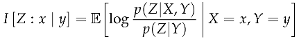
(Predictive Contrast Information). Predictive contrast information measures the information gained about the future target from observing the specific present source in the specific past context .
Since it is equivalent to the relative entropy from to , it measures the degree to which you can distinguish from when is the case. So we have just observed the specific present y, which has some effect on the future, represented by . The present state of the world is represented as and the previous state of the world is represented as . Predictive information is then the number of extra bits needed to describe the current state of the world in terms of the previous state of the world. As such, When this quantity is low, incorporating the present does not change the distribution much over what it looked like using only the past. The future has not changed due to observing the present. When this quantity is high, incorporating the present dramatically changes the distribution of the future over what it was before observing the present. The present provides a lot of information about the future.
5.2. Connective Contrast Information
Connective contrast information indicates the degree to which the past informs the future more than what the present already does. Similar to memory gap [42], it measures the degree to which knowledge of the present separates the past and the future. As such, it can also be considered as measuring how non-Markovian the process is at the present moment in time. For instance, for Markov processes, all information in the past about the future is contained in the present, so connective information will always be zero for Markov processes, though for higher-order Markov processes, this may not be the case.
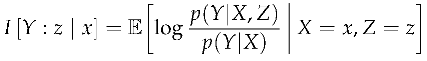
Definition 9
(Connective Contrast Information). Connective contrast information measures the information gained about the future target from observing a specific past source in the specific present context .
It measures the degree to which you can distinguish from when is the case. It measures the degree to which the present aids or hinders the past in informing the future. If most information about the future is contained in the present, then this quantity will be low. When this quantity is high, the present serves as a conduit of information from the past to the future.
5.3. Reflective Contrast Information
Reflective contrast information measures how knowledge of the future impacts the present in the context of the past. It can be thought of as measuring hindsight, since the specific future source occurs after the target present. Intuitively, sometimes the significance of an event is only appreciated after the fact, where the outcomes of subsequent events make clear the importance of some previous event. Though not a perfect analogy, suppose that today corresponds to the future and yesterday corresponds to the present. If knowing what you know today would change what you did yesterday, then there would be high reflective contrast information. If you wouldn’t change a thing, then there is low reflective contrast information.
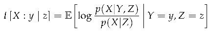
Definition 10
(Reflective Contrast Information). Reflective contrast information measures the information gained about the present target from observing a specific future source in the specific past context .
This quantity is low when knowledge of the future does not change the present in the context of the past. The lower the reflective contrast information, the more that information flows in a single direction from the past to the future. When this is high, knowledge of the future provides a lot of information about the present more than what the past already provided.
5.4. Backward Temporal Variants
The three previous variants of contrast information are considered as variants of forward contrast information because the temporal regime associated with the context occurs before the temporal regime associated with the target. When the context occurs after the target, then we have the backward variants of contrast information. The backward variants can be thought of as reversing the arrow of time and measuring the forward contrast information of this reverse version. Each of the backward variants are paired with their forward variants by interchanging the appropriate regimes. We include these measures merely for completeness.
Definition 11
(Backward Contrast Information). The variants of backward contrast information are analogous to their forward counterparts, except that the regime in the context occurs after the regime in the target.
- Backward Predictive Contrast Information
- Backward Connective Contrast Information
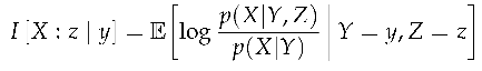
- Backward Reflective Contrast Information
5.5. Terminology
Since contrast information is just one form of specific information, you might wonder why we insist on calling it contrast information at all. Why introduce new terminology when contrast information is exactly specific information? The reason for this is twofold.
First, the random variables and specific outcomes found in contrast information always correspond to three temporal regimes, not just any three random variables. The sequentiality of these variables is at the very core of the semantics of contrast information. If we are instead referring only to specific information, there is no assumption of sequentiality, and so the variables present in the expression do not carry temporal semantics in the same way. By referring to contrast information instead, we are indicating that the quantities involved are parts of a process. Since sequentiality is so important in information dynamics, it makes sense to use terminology and notation that integrates sequentiality as well.
The second reason is more heuristic. Since in the context of contrast information we always indicate the past, present, and future with specific variables names , we gain a lot of notational utility by distinguishing contrast information from specific information. Whenever you see a see Z in regard to contrast information, you immediately know that it refers to the future. Whereas more generally with specific information, a random variable named Z does not necessarily carry that meaning, and it would have to be specified explicitly with each usage to avoid confusion.
6. Constrast Information of Some Stochastic Processes
6.1. Contrast Information of a Discrete-Time Markov Process
A discrete-time Markov Chain (DTMC) is a discrete-time stochastic process over a finite set of discrete states possessing the Markov property. In our case, the future is independent of the past given the present.
When the DTMC is stationary, the transition probabilities between states remained fixed over time, and the process can be represented as a transition matrix P, The entry indexed by row j and column k represents the conditional probability that, given you are in state k, you will transition to state j in the next time step, with each column summing to 1, i.e. where is a row vector of ones.2 When S is ergodic, aperiodic, and irreducible, we can also represent the stationary distribution as the vector so that the entry of is the stationary probability . The reverse transition matrix R has entries representing the probability that, given you are in state k, you just transitioned from state j. The entries of the reverse transition matrix can be determined from the forward transition matrix P and stationary distribution , as , or in matrix form, where .
By selecting the appropriate temporal regimes for X, Y, and Z, we can use the transition matrices P and R to calculate all the variants of contrast information. Consider the regimes j steps into the past and k steps into the future.
We can express the -step contrast information as follows, where is the transition matrix P multiplied n times, and is a one-hot vector representation of the state x.
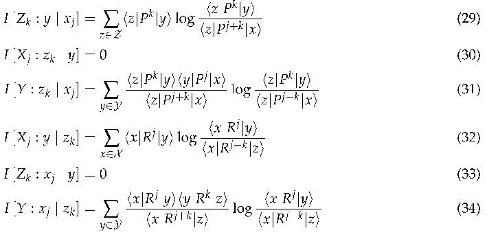
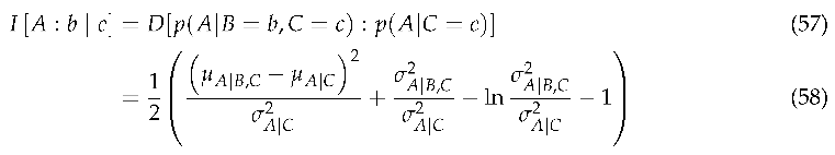
The forward predictive and reflective contrast information are illustrated in Figure 1 for a musical melody.
6.2. Contrast Information of a Continuous-Time Markov Process
A continuous-time Markov chain (CTMC) [43] is the continuous-time version of a DTMC, where future is independent of the past given the present. When the CTMC is stationary, the transition matrix P after some (scalar) time t can be expressed as the matrix exponential of a rate matrix Q.
Like the transition matrix P for the DTMC, the rate matrix Q determines the behaviour of a stationary CTMC, with and . The stationary distribution of the CTMC obeys and allows us to determine the reverse rate matrix where .
By selecting temporal regimes X, Y, and Z as points, we can use the rate matrices Q and to calculate all the variants of contrast information. Consider the regimes with time u into the past and time v into the future.
We can express the contrast information as follows, where is the matrix exponential, and is a one-hot vector representation of the state x.
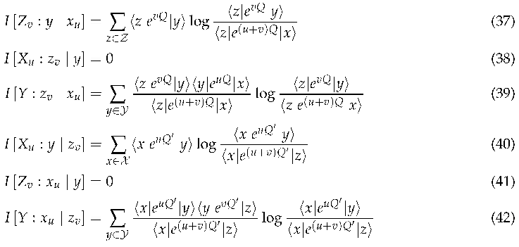
The forward predictive and reflective contrast information are illustrated in Figure 2 for a musical melody.
6.3. Discrete-Time Gaussian Process
A Gaussian process is a stochastic process [44] where all finite-dimensional marginals are multivariate Gaussian distributions. A multivariate Gaussian S is defined according to its mean vector and covariance matrix ,
and has probability density when , i.e., is symmetric positive definite.
The general formula for contrast information of Gaussian processes can be derived from the KL divergence between two (multivariate) Gaussians [45], over the target A with length n.
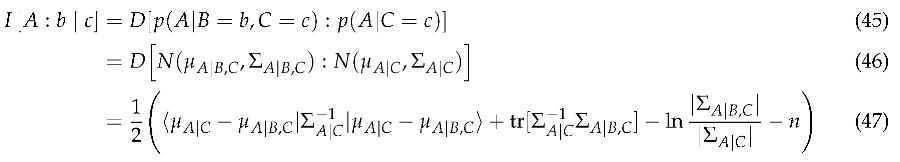 where S is partioned into target A, source B, and context C, with associated mean vector and block covariance matrix .
where S is partioned into target A, source B, and context C, with associated mean vector and block covariance matrix .
The conditional distribution of the target A given the source B and context C is also a multivariate Gaussian, with the following mean vector and covariance matrix.
Similarly, the conditional distribution of the target A given only the context C is also multivariate Gaussian, with corresponding mean vector and covariance matrix.
For stationary discrete-time Gaussian processes (DTGP), the covariance matrix can be expressed in terms of a discrete-time autocovariance function , i.e., each entry in the covariance matrix .
Defining the temporal regimes as extended j units of time into the past and k units of time into the future, the temporal regimes can be plugged in to the context, source, and target, to yield the different desired variants of contrast information.
The forward predictive, reflective, and connective contrast information are illustrated in Figure 3 for a musical melody.
6.4. Continuous-Time Gaussian Process
A continuous-time Gaussian processes (CTGP) [46] are essentially the same as DTGPs, except that a covariance operator or kernel function may be used to deal with the continuity of the temporal domain. When the CTGP is stationary, then we can use a continuous-time autocovariance function to describe its covariance, as opposed to the discrete-time autocovariance used for DTGPs.
Suppose we define the source B and target C as points in time. This may be useful when we have heterogeneously sampled data that is not continuously observed. In this case, the temporal regimes must all be associated with single points in time,
and the contrast information for Gaussian processes simplifies to the following.
The different variants of contrast information can be determined by plugging in the relevant temporal regimes. The forward predictive, reflective, and connective contrast information are illustrated in Figure 4 for a musical melody.
7. Contrast Information in IDyOMS
7.1. Information Dynamics of Multidimensional Sequences (IDyOMS)
The Information Dynamics of Multidimensional Sequences (IDyOMS)3 is an implementation, and generalisation, of the Information Dynamics of Music (IDyOM: [2]) for use with any kind of discrete multidimensional sequence data: sequences of points in multidimensional feature space, each represented by a finite number of discrete feature values. IDyOMS determines the information content of each sequence event using Markov models of varying orders (up to a specified order bound) for a chosen combination of features (dimensions). Probability distributions over a given dimension are computed using Prediction by Partial Matching (PPM: [47]) for each sequence event. These individual feature models, referred to a viewpoint models [14], are then combined according to their predictive power (the entropy of the distribution) to give the overall information dynamics of a sequence in terms of evolving information content and entropy.
As previously discussed, such variable order, multiple viewpoint systems are strong cognitive models of unexpectedness, uncertainty and chunking in the perception of discrete musical sequences. With the ultimate goal of generalising these models for use with equivalent continuous representations using contrast information, we substituted information content for contrast information in IDyOMS and compared the resulting information dynamic profiles of a corpus of 152 folk melodies from Nova Scotia, Canada. These melodies comprise sequences of events, each represented by their pitch and duration. We separately examined viewpoint models for these features (CPITCH and DUR), as well as a combined model (referred to as the linked viewpoint model [18,48] CPITCH × DUR).
7.2. Results
Pearson () and Spearman () correlations were calculated between information content and forward predictive contrast information (Table 2) and between entropy and expected forward predictive contrast information (Table 3) for the three viewpoint models (CPITCH, DUR and CPITCH×DUR) for a range or order bounds (0-10). The correlations vary significantly across both viewpoint models and order bounds.
Correlations tend to increase as the order increases. The tables in include correlations of the zeroth order models (static models which do not use past events to estimate probabilities) where the entropy and expected forward predictive contrast information are constant (so Spearman does not apply) while the information content and forward predictive contrast information reflect the maximum likelihood of a single feature value occurring in the corpus. Intuitively we understand that increasing the order bound (the maximum number of past events considered in the prediction) has the effect of decreasing the relative contribution to the information profiles of the distribution over future events, and so contrast information approaches information content.
Correlations were higher for the simple viewpoint models CPITCH and DUR and lower for the linked viewpoint model CPITCH × DUR. This is due the increased alphabet size of the linked (Cartesian product) feature value domain relative to the corpus size, and the resultant lower probabilities and higher contribution of the distribution over the future.
Some differences are present between the two correlations used. While high Pearson correlation indicates a strong overall similarity in the shapes of information profiles, high Spearman correlation indicates the degree to which the information profiles have peaks in the same locations. This is highly desirable if contrast information is to be used in place of information content and entropy in future work on segment boundary detection.
Overall, these results show that in many cases, using contrast information in place of information content and entropy in IDyOMS would not significantly impact the downstream cognitive modelling methodologies for segment boundary detection. However, this is clearly highly dependent on the viewpoint models and order bounds used. Being that the major difference between the two methods for computing information profiles is the contribution of distributions over future events, subsequent application of IDyOMS for cognitive modelling using contrast information should take into account the order bound and alphabet size of a viewpoint model relative to the size of the corpus.
8. Discussion
8.1. Contributions
We have presented a set of novel information measures that are well-suited for use in a cognitive model based on information dynamics of continuous signals, such as our planned IDyOT model. We have presented some useful properties of the new measures. We have shown that there exists a good correlation, particularly in rank order, between the measures used in the IDyOM system and the discrete version of our measures. Since IDyOM is already empirically demonstrated to be a strong cognitive model, it follows that at least the discrete version of our new measures will serve effectively as a cognitive model also; therefore, it is reasonable to expect that the continuous versions will do the same.
8.2. Future Work
Immediate opportunities for further work in this area are as follows:
- Boundary Entropy
- The first application of the new measures will be in replicating prior segmentation work in music. This will require adaptation of the information profile peak picking algorithms for use on contrast information. Subsequently, we will test the continuous measures on speech, using the TIMIT dataset4.
- Continuous-state IDyOMS
- We will extend our IDyOMS software to allow for continuous states, thus extending its representational reach in music and other domains. This will require the substituting the PPM algorithm with models of continuous feature dimensions, as well as methods for combining viewpoint models based on contrast information rather than entropy.
- Neural correlates
- We aim to collaborate with colleagues in neuroscience to investigate whether and how the neural correlates of perceived sound correspond with IDyOT representations, with a view to making the system more human-like.
- Spectral Knowledge Representation
- We will further develop the idea of Spectral Knowledge Representation [36] to allow our system to reason using the symbols identified by segmentation.
In the longer term, we will continue to develop the components required for the IDyOT cognitive architecture, working towards a full implementation.
Author Contributions
Conceptualization, S.H. and G.W.; methodology, S.H., N.H, and G.W.; software, S.H. and N.H.; validation, S.H. and N.H.; formal analysis, S.H.; investigation, S.H. and N.H.; data curation, N.H.; writing—original draft preparation, S.H., N.H.; writing—review and editing, S.H., N.H. and G.W.; supervision, G.W.; project administration, G.W. All authors have read and agreed to the published version of the manuscript.
Funding
This research received funding from the Flemish Government under the
Institutional Review Board Statement
Not applicable.
Informed Consent Statement
Not applicable.
Acknowledgments
We are grateful for feedback from our colleagues in the Computational Creativity Lab at the VUB.
Conflicts of Interest
The authors declare no conflicts of interest. The funders had no role in the design of the study; in the collection, analyses, or interpretation of data; in the writing of the manuscript; or in the decision to publish the results.
References
- Cover, T.M.; Thomas, J.A. Elements of Information Theory, 2 ed.; John Wiley & Sons, Inc), 2006.
- Pearce, M.T. The Construction and Evaluation of Statistical Models of Melodic Structure in Music Perception and Composition. PhD thesis, Department of Computing, City University, London, London,UK, 2005.
- Pearce, M.T.; Wiggins, G.A. Auditory Expectation: The Information Dynamics of Music Perception and Cognition. Topics in Cognitive Science 2012, 4, 625–652. [Google Scholar] [CrossRef]
- Abdallah, S.A.; Plumbley, M.D. Information dynamics: Patterns of expectation and surprise in the perception of music. Connection Science, 2009. In press.
- Agres, K.; Abdallah, S.; Pearce, M. Information-Theoretic Properties of Auditory Sequences Dynamically Influence Expectation and Memory. Cognitive Science, 2017, pp. 1–34. [CrossRef]
- MacKay, D.J.C. Information Theory, Inference, and Learning Algorithms; Cambridge University Press: Cambridge, UK, 2003. [Google Scholar]
- Friston, K. The free-energy principle: A unified brain theory? Nature Reviews Neuroscience 2010, 11, 127–138. [Google Scholar] [CrossRef] [PubMed]
- Schmidhuber, J. Formal Theory of Creativity, Fun, and Intrinsic Motivation (1990–2010). Autonomous Mental Development, IEEE Transactions on 2010, 2, 230–247. [Google Scholar] [CrossRef]
- Clark, A. Whatever next? Predictive brains, situated agents, and the future of cognitive science. Behavioral and Brain Sciences 2013, 36, 181–204. [Google Scholar] [CrossRef] [PubMed]
- Wiggins, G.A. Creativity, Information, and Consciousness: the Information Dynamics of Thinking. Physics of Life Reviews 2020, 34–35, 1–39. [Google Scholar] [CrossRef] [PubMed]
- Wiggins, G.A. Artificial Musical Intelligence: computational creativity in a closed cognitive world. In Artificial Intelligence and the Arts: Computational Creativity in the Visual Arts, Music, 3D, Games, and Artistic Perspectives; Computational Synthesis and Creative Systems, Springer International Publishing, 2021.
- Huron, D. Sweet Anticipation: Music and the Psychology of Expectation; Bradford Books, MIT Press: Cambridge, MA, 2006. [Google Scholar]
- Conklin, D. Prediction and Entropy of Music. Master’s thesis, Department of Computer Science, University of Calgary, Canada, 1990.
- Conklin, D.; Witten, I.H. Multiple Viewpoint Systems For Music Prediction. Journal of New Music Research 1995, 24, 51–73. [Google Scholar] [CrossRef]
- Pearce, M.T. Statistical learning and probabilistic prediction in music cognition: mechanisms of stylistic enculturation. Annals of the New York Academy of Sciences 2018, 1423, 378–395. [Google Scholar] [CrossRef] [PubMed]
- Moffat, A. Implementing the PPM data compression scheme. IEEE Transactions on Communications 1990, 38, 1917–1921. [Google Scholar] [CrossRef]
- Bunton, S. Semantically Motivated Improvements for PPM Variants. The Computer Journal 1997, 40, 76–93. [Google Scholar] [CrossRef]
- Pearce, M.T.; Conklin, D.; Wiggins, G.A. Methods for Combining Statistical Models of Music. In Computer Music Modelling and Retrieval; Wiil, U.K., Ed.; Springer Verlag: Heidelberg, Germany, 2005; pp. 295–312. [Google Scholar]
- Pearce, M.T.; Wiggins, G.A. Expectation in Melody: The Influence of Context and Learning. Music Perception 2006, 23, 377–405. [Google Scholar] [CrossRef]
- Pearce, M.T.; Herrojo Ruiz, M.; Kapasi, S.; Wiggins, G.A.; Bhattacharya, J. Unsupervised Statistical Learning Underpins Computational, Behavioural and Neural Manifestations of Musical Expectation. NeuroImage 2010, 50, 303–314. [Google Scholar] [CrossRef] [PubMed]
- Hansen, N.C.; Pearce, M.T. Predictive uncertainty in auditory sequence processing. Frontiers in Psychology 2014, 5. [Google Scholar] [CrossRef] [PubMed]
- Pearce, M.T.; Wiggins, G.A. Evaluating cognitive models of musical composition. Proceedings of the 4th International Joint Workshop on Computational Creativity; Cardoso, A., Wiggins, G.A., Eds.; Goldsmiths, University of London: London, 2007; pp. 73–80. [Google Scholar]
- Pearce, M.T.; Müllensiefen, D.; Wiggins, G.A. The role of expectation and probabilistic learning in auditory boundary perception: A model comparison. Perception 2010, 39, 1367–1391. [Google Scholar] [CrossRef] [PubMed]
- Wiggins, G.A. Cue Abstraction, Paradigmatic Analysis and Information Dynamics: Towards Music Analysis by Cognitive Model. Musicae Scientiae 2010, Special Issue: Understanding musical structure and form: papers in honour of Irène Deliège, 307–322.
- Wiggins, G.A. “Iletthemusicspeak”:cross-domainapplicationofacognitivemodelofmusicallearning. In Statistical Learning and Language Acquisition; Rebuschat, P., Williams, J., Eds.; Mouton De Gruyter: Amsterdam, NL, 2012; pp. 463–495. [Google Scholar]
- Griffiths, S.S.; McGinity, M.M.; Forth, J.; Purver, M.; Wiggins, G.A. Information-Theoretic Segmentation of Natural Language. Proceedings of the 2nd Workshop on AI and Cognition, 2015.
- Tan, N.; Aiello, R.; Bever, T.G. Harmonic structure as a determinant of melodic organization. Memory and Cognition 1981, 9, 533–9. [Google Scholar] [CrossRef] [PubMed]
- Chiappe, P.; Schmuckler, M.A. Phrasing influences the recognition of melodies. Psychonomic Bulletin & Review 1997, 4, 254–259. [Google Scholar]
- Wiggins, G.A.; Sanjekdar, A. Learning and consolidation as re-representation: revising the meaning of memory. Frontiers in Psychology: Cognitive Science 2019, 10. [Google Scholar] [CrossRef] [PubMed]
- Shannon, C. A mathematical theory of communication. Bell System Technical Journal 1948, 27, 379–423. [Google Scholar] [CrossRef]
- Large, E.W. A generic nonlinear model for auditory perception. In Auditory Mechanisms: Processes and Models; Nuttall, A.L., Ren, T., Gillespie, P., Grosh, K., de Boer, E., Eds.; World Scientific: Singapore, 2006; pp. 516–517. [Google Scholar]
- Spivey, M. The Continuity of Mind; Oxford University Press, 2008.
- Kraus, N.; Nicol, T. Brainstem Encoding of Speech and Music Sounds in Humans. In The Oxford Handbook of the Auditory Brainstem; Oxford University Press, 2019; pp. (on–line version). [CrossRef]
- Bellier, L.; Llorens, A.; Marciano, D.; Gunduz, A.; Schalk, G.; Brunner, P.; Knight, R.T. Music can be reconstructed from human auditory cortex activity using nonlinear decoding models. PLoS Biol 2023, 21, e3002176. [Google Scholar] [CrossRef]
- Pasley, B.N.; David, S.V.; Mesgarani, N.; Flinker, A.; Shamma, S.A.; Crone, N.E.; Knight, R.T.; Chang, E.F. Reconstructing Speech from Human Auditory Cortex. PLoS Biol 2023, 10, e1001251. [Google Scholar] [CrossRef]
- Homer, S.T.; Harley, N.; Wiggins, G.A. The Discrete Resonance Spectrogram: a novel method for precise determination of spectral content. In preparation.
- Caticha, A. Relative Entropy and Inductive Inference. AIP Conference Proceedings, 2004, Vol. 707, pp. 75–96, [physics/0311093]. [CrossRef]
- Caticha, A. Entropic Inference and the Foundations of Physics; University of Albany – SUNY, 2012.
- Eckhorn, R.; Pöpel, B. Rigorous and Extended Application of Information Theory to the Afferent Visual System of the Cat. I. Basic Concepts. Kybernetik, 16, 191–200. [CrossRef]
- DeWeese, M.R.; Meister, M. How to Measure the Information Gained from One Symbol. Network: Computation in Neural Systems, 1999.
- Good, I.J. Good Thinking: The Foundations of Probability and Its Applications; University of Minnesota Press, 1983.
- Braverman, M.; Chen, X.; Kakade, S.; Narasimhan, K.; Zhang, C.; Zhang, Y. Calibration, Entropy Rates, and Memory in Language Models. Proceedings of the 37 th International Conference on Machine Learning, 2020.
- Anderson, W.J. Continuous-Time Markov Chains; Springer Series in Statistics, Springer New York, 1991. [CrossRef]
- Brockwell, P.J.; Davis, R.A. Time Series: Theory and Methods; Springer Series in Statistics, Springer New York, 1991. [CrossRef]
- Soch, J. ; Maja.; Monticone, P.; Faulkenberry, T.J.; Kipnis, A.; Petrykowski, K.; Allefeld, C.; Atze, H.; Knapp, A.; McInerney, C.D.; Lo4ding00.; others. The Book of Statistical Proofs (Version 2023), 2024. [CrossRef]
- Brockwell, P.; Davis, R.; Yang, Y. Continuous-Time Gaussian Autoregression. Statistica Sinica, 17, 63–80.
- Cleary, J.; Witten, I. Data Compression Using Adaptive Coding and Partial String Matching. IEEE Transactions on Communications 1984, 32, 396–402. [Google Scholar] [CrossRef]
- Hedges, T.; Wiggins, G.A. The Prediction of Merged Attributes with Multiple Viewpoint Systems. Journal of New Music Research 2016, 45, 314–332. [Google Scholar] [CrossRef]
| 1 | We use this joint term because it is not yet clear to us where the boundary between the mind and the brain lies, if indeed there is one. |
| 2 | Here, we represent the transitions using a right stochastic matrix, though it is also common to see a left stochastic matrix representing the transition matrix. We use the right stochastic matrix representation so that we can use Dirac notation with the standard semantics, where a column vector corresponds to a state, as opposed to row vector with the left stochastic matrix. |
| 3 | |
| 4 |
Figure 1.
An example of the contrast information associated with a discrete-time, discrete-state stochastic process. In Figure a), a MIDI representation of a folk melody is represented as a discrete-time process through a uniform sampling in time of the data. The discrete state space of the process is inhabited by the MIDI pitch numbers. Note that, though the visualization represents the pitches as an ordered set, we treat the pitches as an unordered set of discrete states. By treating all melodies in the corpus as instances of the same stationary first-order DTMC, the maximum likelihood estimate of the transition matrix of the DTMC was found. In Figures b) and c), the forward predictive contrast information profile and forward reflective contrast information profile are shown for the melody in Figure a), calculated using the estimated DTMC. Each bar is centered on the present Y, where the past X is the immediately previous pitch, and the future Z is the immediately next pitch. The connective contrast information is omitted here since it is always zero for Markov processes.
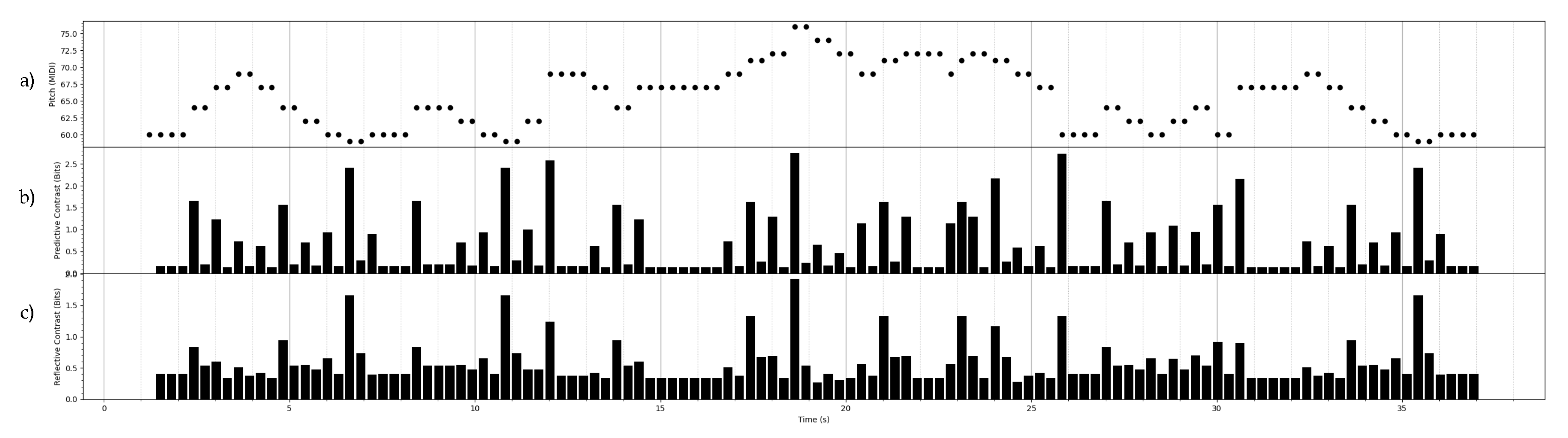
Figure 2.
An example of the contrast information associated with a continuous-time, discrete-state stochastic process. In Figure a), a MIDI representation of a folk melody is represented as a continuous-time process, where the onset of a state is indicated by a triangle, and duration of a state is indicated by the horizontal line. The discrete state space of the process is inhabited by the MIDI pitch numbers. Note that, though the visualization represents the pitches as an ordered set, we treat the pitches as an unordered set of discrete states. By treating all melodies in the corpus as instances of the same stationary CTMC, the maximum likelihood estimate of the rate matrix of the CTMC was found. In Figure b), the forward predictive contrast information profile is shown. The present Y is located at the most recent pitch onset, and the past X is located at the pitch onset immediate before Y. Each point on the profile curve is centered on the future Z, which varies in time from the most recent pitch onset (Y) to the next pitch onset, at which point the past and present shift forward to the next pitch onsets. In Figure c), the forward reflective contrast information profile is shown. The past X is located at the most recent pitch onset. The future Z is located at the next pitch onset. Each point in the profile curve is centered on the present Y, which varies in time from the most recent pitch X to next pitch Z, at which point the past and future shift forward to the next pitch onsets. The connective contrast information is omitted here since it is always zero for Markov processes.
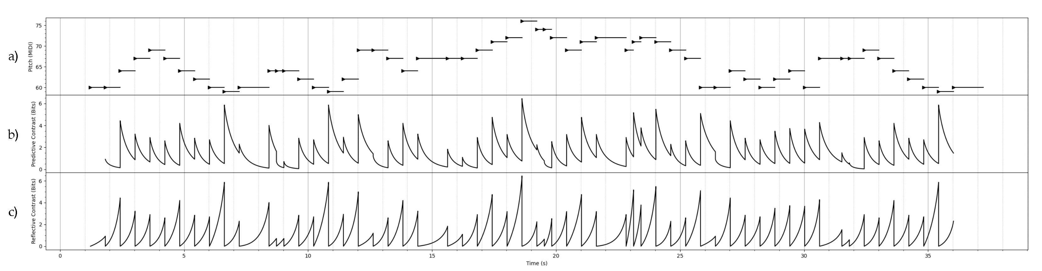
Figure 3.
An example of the contrast information associated with a discrete-time, continuous-state stochastic process. In Figure a), a MIDI representation of a folk melody is represented as a discrete-time process through a uniform sampling in time of the data. The continuous state space of the process is inhabited by the frequencies associated with each MIDI pitch. By treating all melodies in the corpus as instances of the same stationary Gaussian process, the maximum likelihood estimates for the mean and autocovariance of the Gaussian process were found. In Figures b), c) and d), the contrast information profiles are calculated using the estimated DTGP. Each bar is centered on the present Y, where the past X is the immediately previous pitch, and the future Z is the immediately next pitch. In this case, using longer duration regimes for the past and future resulted in very similar profiles, so the profiles shown here are generally representative. Note the scale of the connective contrast is much lower than the other the predictive and reflective contrast.
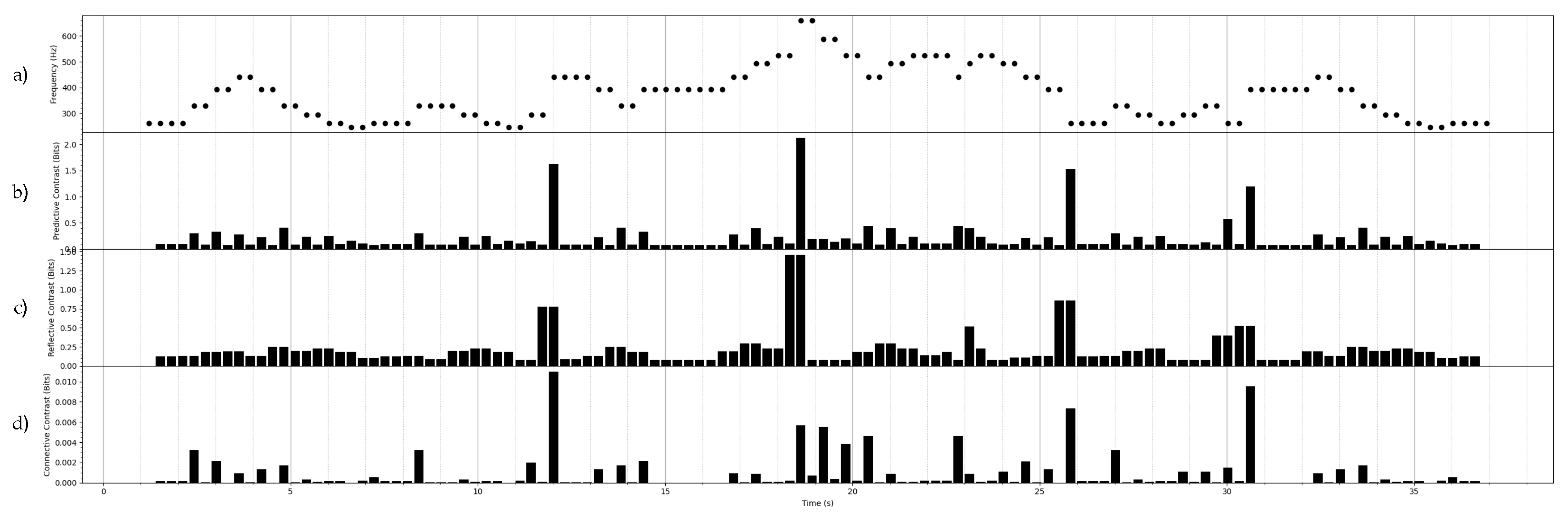
Figure 4.
An example of the contrast information associated with a continuous-time, continuous-state stochastic process. In Figure a), a MIDI representation of a folk melody is represented as a continuous-time process, where the onset of a state is indicated by a triangle, and duration of a state is indicated by the horizontal line. The continuous state space of the process is inhabited by the frequencies associated with each MIDI pitch. By treating all melodies in the corpus as instances of the same stationary Gaussian process, the maximum likelihood estimates for the mean and autocovariance of the discrete-time Gaussian process were found. The discrete-time autocovariance function was then fit with a high degree polynomial to give a continuous-time autocovariance function. In Figure b), the forward predictive contrast information profile is shown. The present Y is located at the most recent pitch onset, and the past X is located at the pitch onset immediate before Y. Each point on the profile curve is centered on the future Z, which varies in time from the most recent pitch onset (Y) to the next pitch onset, at which point the past and present shift forward to the next pitch onsets. In Figure c), the forward reflective contrast information profile is shown. The past X is located at the most recent pitch onset. The future Z is located at the next pitch onset. Each point in the profile curve is centered on the present Y, which varies in time from the most recent pitch X to next pitch Z, at which point the past and future shift forward to the next pitch onsets. In Figure d), the forward connective contrast information profile is shown. The past, present, and future follow the same scheme as described for forward predictive contrast information in Figure b). Note the scale of the connective contrast is much lower than the other the predictive and reflective contrast.
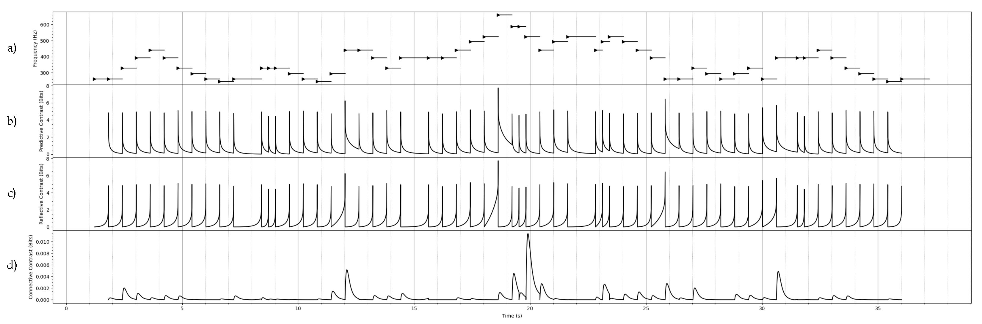

Table 1.
Sequence notation schemes for sequences of random variables.
| Regime | Continuous | Notation | Discrete | Notation |
|---|---|---|---|---|
| Past | X | X | ||
| Near Past | ||||
| Point Past | ||||
| Present | Y | Y | ||
| Point Future | ||||
| Near Future | ||||
| Future | Z | Z |
Table 2.
Correlation between information content and forward predictive contrast information. Zeroth order model (i.e., constant distribution) is included to emphasise the difference between this and information dynamic models.
Table 2.
Correlation between information content and forward predictive contrast information. Zeroth order model (i.e., constant distribution) is included to emphasise the difference between this and information dynamic models.
| CPITCH | DUR | CPITCH x DUR | ||||
|---|---|---|---|---|---|---|
| Order | ||||||
| 0 | 0.86 | 0.88 | 0.89 | 1.00 | -0.83 | -0.82 |
| 1 | 0.85 | 0.86 | 0.72 | 0.51 | 0.34 | 0.38 |
| 2 | 0.76 | 0.77 | 0.70 | 0.66 | 0.45 | 0.47 |
| 3 | 0.73 | 0.76 | 0.70 | 0.69 | 0.23 | 0.28 |
| 4 | 0.75 | 0.81 | 0.71 | 0.72 | 0.19 | 0.33 |
| 5 | 0.77 | 0.86 | 0.73 | 0.78 | 0.23 | 0.39 |
| 6 | 0.78 | 0.88 | 0.74 | 0.80 | 0.32 | 0.45 |
| 7 | 0.80 | 0.90 | 0.75 | 0.82 | 0.45 | 0.50 |
| 8 | 0.82 | 0.91 | 0.75 | 0.84 | 0.58 | 0.54 |
| 9 | 0.84 | 0.92 | 0.76 | 0.86 | 0.66 | 0.57 |
| 10 | 0.85 | 0.92 | 0.77 | 0.87 | 0.69 | 0.60 |
Table 3.
Correlation between entropy and expected forward predictive contrast information. Zeroth order model (i.e., constant distribution) is included to emphasise the difference between this and information dynamic models.
Table 3.
Correlation between entropy and expected forward predictive contrast information. Zeroth order model (i.e., constant distribution) is included to emphasise the difference between this and information dynamic models.
| CPITCH | DUR | CPITCH x DUR | ||||
|---|---|---|---|---|---|---|
| Order | ||||||
| 0 | 1.00 | - | 1.00 | - | 1.00 | - |
| 1 | 0.20 | -0.06 | 0.36 | -0.48 | -0.28 | -0.23 |
| 2 | 0.24 | 0.28 | 0.31 | -0.14 | 0.06 | 0.33 |
| 3 | 0.51 | 0.50 | 0.40 | 0.29 | 0.27 | 0.36 |
| 4 | 0.67 | 0.68 | 0.44 | 0.29 | 0.34 | 0.46 |
| 5 | 0.73 | 0.81 | 0.50 | 0.42 | 0.37 | 0.53 |
| 6 | 0.75 | 0.89 | 0.55 | 0.49 | 0.42 | 0.59 |
| 7 | 0.77 | 0.93 | 0.60 | 0.60 | 0.54 | 0.64 |
| 8 | 0.80 | 0.95 | 0.64 | 0.70 | 0.68 | 0.68 |
| 9 | 0.83 | 0.96 | 0.66 | 0.76 | 0.77 | 0.71 |
| 10 | 0.85 | 0.97 | 0.67 | 0.80 | 0.81 | 0.73 |
Disclaimer/Publisher’s Note: The statements, opinions and data contained in all publications are solely those of the individual author(s) and contributor(s) and not of MDPI and/or the editor(s). MDPI and/or the editor(s) disclaim responsibility for any injury to people or property resulting from any ideas, methods, instructions or products referred to in the content. |
© 2024 by the authors. Licensee MDPI, Basel, Switzerland. This article is an open access article distributed under the terms and conditions of the Creative Commons Attribution (CC BY) license (http://creativecommons.org/licenses/by/4.0/).
Copyright: This open access article is published under a Creative Commons CC BY 4.0 license, which permit the free download, distribution, and reuse, provided that the author and preprint are cited in any reuse.


