
Submitted:
22 April 2024
Posted:
23 April 2024
You are already at the latest version
Abstract
Some optimal control problems need metaheuristics in searching for the optimal solution, especially when the process has certain characteristics like the Photobioreactor for Algae Growth (distributed parameter, nonlinearities, etc.). Particle Swarm Optimization (PSO) algorithms within control structures are a realistic approach; their task is often to predict the optimal control values working with a process model (PM). Owing to numerous numerical integrations, there is a big computational effort that is reflected in a large controller execution time. The authors propose to replace the PSO predictor with a machine learning model that has “learned” the quasi-optimal behavior of the couple (PSO, PM); the training data is obtained through closed-loop simulations over the control horizon. The new controller should preserve the process’s quasi-optimal control. In identical conditions, the process evolutions must also be quasi-optimal. The multiple Linear Regression and the Regression Neural Networks were considered as predicting models. The paper first proposes algorithms for collecting and aggregating data sets for the learning process. Algorithms for constructing the machine learning models, implementing the controllers, and closed-loop simulations are also proposed. The simulations prove that the two machine learning predictors have learned the PSO predictor’s behavior such that the process evolves almost identically. The resulting controllers’ execution time drastically decreased while keeping their optimality.
Keywords:
particle swarm optimization
; machine learning
; optimal control
; simulation
1. Introduction
A common task in process engineering is to control processes whose quality is evaluated through a performance index. When the process model has certain mathematical properties, theoretical control laws can be adopted for implementation; on the contrary, when the process model is uncertain, incomplete, imprecise or has profound nonlinearities, metaheuristic algorithms (MAs) like Evolutionary Algorithms, Particle Swarm Optimization etc, within a suitable control structure, could be successfully used [1,2,3]. Control engineering afforded numerous examples where metaheuristics were used [4,5,6,9,16] owing to their robustness and capacity to deal with complex processes.
The role of an MA within a controller is usually to predict the optimal control values at each sampling period, but first, it searches for the optimal value. For example, the PSO algorithm follows its optimization mechanism using particles and the internal PM.
A control structure fitting this type of controller is Receding Horizon Control (RHC) [10,12,13]. This structure is suitable for implementing solutions to Optimal Control Problems (OCPs); it includes an internal Process Model (PM) [14,15,16].
A predilect research topic for the authors was implementing the prediction module within an RHC structure employing MAs. The results are partially reflected in previous works [16,19,21]. The robustness, efficiency and usability of MAs inside a controller have a price to pay: the controller’s execution time. The optimization mechanism and the numerous PM’s numerical integrations involve a relatively “long” time to find the optimal value after a convergence process. That is why this approach is mainly suitable for slow processes when the predictions’ computation time is smaller than the sampling period [27,28]. Decreasing the predictor’s execution time is a challenge [19,21] because it could extend the applicability of controllers using MAs. This work goes in the same direction but involves a new technique: using machine learning (ML) to emulate predictors based on MAs. Recently, we have proposed Linear Regression (LR) predictors that are “equivalent” in a certain sense to predictors based on Evolutionary Algorithms (Eas) [11]. In our opinion, the present work goes beyond the predictor’s execution time decrease and opens a perspective to emulate and replace optimization structures generally.
This paper deals with OCPs having final costs and solutions involving PSO predictions. To continue the work presented in [11], we shall consider the equivalence mentioned above and implement Regression Neural Networks (RNN) predictors., besides the LR ones.
Along this paper we have recourse to a specific OCP to make the explanations easy to follow by the reader. In paper [13], for the optimal control of a specific photobioreactor (PBR) lighted for algae growth, we have presented a solution in the same context, RHC and predictions based on PSO. We shall take over the PSO predictor already constructed in [13]; employing this one, we shall generate new ML predictors. Data generated by simulation modules, already developed previously, is stored or recorded. This data will be needed to train and test the ML models. Some results from [13] will be reported in this paper for comparison (Section 7.1).
Section 2 recalls the general approach developed in previous work [7,8,16] to solve such problems using PSO algorithms. Besides the recall of the PBR problem’s statement, Section 2 also introduces the notations and formulas that keep the presentation self-contained.
Section 3 answers the following two main questions:
- What data is needed to capture the optimal (quasi-optimal) behaviour of the couple (PSO, PM)?
- How are the datasets for the ML algorithms generated?
The PSO prediction module, included in the controller, is available from our previous work, which has already solved the PBR problem. Section 3 presents an algorithm carrying out the closed-loop simulation over the control horizon using the PSO predictor. A mandatory hypothesis is that the real process and the internal PM are considered identical because the data recorded should capture only the behaviour of the couple (PSO, PM).
At the end of the simulation, the sequence of optimal control values (optimal control profile) and the sequence of state variables (optimal trajectory) can be recorded. The optimal CP and trajectory can be seen as the “signature” data of the optimal solution. Considering together the two sequences, we get a sequence of couples (state, control value), one couple for each sampling period. The simulation program is executed M times (e.g., two hundred times); the two sequences are collected each time and aggregated into a data structure. This data structure expresses the PSO predictor’s experience as a decision-maker; it will be used to obtain the ML models [22,23,24,25,26].
Section 4 presents the general approach to learning the optimal behaviour of the couple (PSO, MP). The learning process is split at the level of each sampling period, and consequently, new data structures are derived for each of them. To each new data structure, which is a collection of couples (state, control value), a generic regression function [17,18,22] is associated. The latter is materialized through an ML regression model devoted to the sampling period at hand, which must be capable of giving accurate predictions.
An ML controller’s systematic design procedure is also proposed. We have to emphasize that the entire design procedure of the ML controller needs only simulations and offline program executions.
In this paper, we consider as regression models only two kinds of models: multiple Linear Regression [29,30,31] and Regression Neural Network [20,22]. Other kinds of models were considered in our studies as well, but only these types of models are relevant to this presentation. Implementing an ML controller, in our context, involves determining a regression model for each sampling period.
Section 5 deals with constructing a set of Linear Regression (LR) models [29,31] that are trained with the data sets constructed in Section 4. A general construction algorithm using the stepwise regression [30] strategy is proposed. A table with the regressions’ coefficients is extracted from the models. The LR Controller is implemented using the LR predictors; it is also integrated into a proposed closed-loop simulation program, allowing us to evaluate the entire approach. Some simulation results are given.
Section 6 proposes a general algorithm for constructing the models using Regression Neural Networks [20]. The training and testing data sets are already determined in Section 4 where they are saved in an external file. A specific closed-loop simulation program is also proposed; it includes the RNN Controller using the RNN predictors. Simulation results are presented for further analysis.
The Discussion Section first answers the following question: Did the two kinds of predictors “learn” the behaviour of the couple (PSO, PM) such that the new process’s evolutions would also be quasi-optimal? To do this, we depicted the new process’s evolutions and displayed some numerical information using the closed-loop simulation programs proposed in Section 5 and Section 6. The simulation results are compared with those already available concerning the PSO predictor. Owing to their generalization ability, both ML controllers make accurate predictions of the control value sent to the process, and the state evolutions are practically identical.
The second question this Section has to answer is: Did the controller’s execution time decrease significantly? Some measures show that it decreased drastically.
The positive answer to both questions proves that the ML controllers are an effective way to avoid the large execution time of the controllers based on PSO while keeping the optimality of the control. This result is important because it extends the possibility of using PSO (or other MA) controllers for processes with smaller time constants.
Special attention was paid to the implementation aspects such that the interested reader could find support to understand and, eventually, reproduce parts of this work or use it in their projects. With this aim in view, all algorithms used in this presentation are implemented, the associated scripts are attached as Supplementary Materials, and all the necessary details are given in the Appendixes.
2. Controllers with Predictions Based on PSO. Connection with Machine Learning Algorithms
Many controlled processes, such as the biochemical processes, are repetitive, like those organized by batches. For efficiency reasons, they generate Optimal Control Problems involving three components:
- The process model can include nonlinearities, imprecise, incomplete, and uncertain knowledge, or correspond to a distributed-parameter system, etc.
- The constraints, such as initial conditions, bound constraints, final constraints, etc.
- The cost function, which should be optimized, leads to a performance index.
To solve such a control problem, we need an adequate control structure which will define the optimal controller. The latter includes a prediction module that calculates the optimal control sequence and the optimal trajectory over the prediction horizon or even until the end of the control horizon. For its work, the predictor uses the PM for a huge number of numerical integrations. In this context, the predictor has a very complex numerical task; that is why a metaheuristic algorithm is often a realistic solution to fulfil this task.
The Receding Horizon Control (RHC) [12,13,16] is a very simple control strategy that can easily integrate a metaheuristic algorithm as a predictor (Figure 1). The authors have studied and simulated the RHC in solving different OCPs in conjunction with the EA or the PSO. The solutions are realistic, they can be used in real-time control, and several techniques can be used to decrease the numerical complexity of the predictor. Nevertheless, the inconvenience is that the control action takes a big part of the sampling period.
An interesting and practical approach, in this context, is to replace the predictor with a Machine Learning algorithm inside the controller. The ML algorithm must emulate the predictor of the RHC structure following its training offline. To emphasize its role, we shall refer to this algorithm as the ML controller. In this work, we have to answer the following questions:
- What does it mean that the ML algorithm must emulate the predictor?
- What are datasets used in training the ML, and how are they obtained?
- What kind of ML model can be used to achieve an appropriate controller?
In paper [13], we have presented the optimal control of a continuously stirred flat-plate photobioreactor (PBR) lighted on a single side for algae growth in the same context: the RHC that uses predictions based on PSO.
In this presentation, all the essential tasks concerning the ML do not need the PM; only the final simulations, which allow us to validate the entire approach, employ the PM. That is why the reader can find in Appendix A the equations modelling the PBR, the constraints and the cost function of the OCP. The PBR is a distributed parameter system, but the PM is converted by discretization into a lumped parameter process. We have solved this problem in the paper [13], adding the discretization constraint, which refers to the input variables:
T is the sampling period, and the final time of the batch equals H∙T. In our example, the input vector has a single component, i.e.
The variable is the intensity of incident light along the kth sampling period.
At every moment , the predictor calculates the optimal control sequence (1) using the usual version of the APSOA (adaptive PSO algorithm) and the PM, which is integrated a large number of times. The optimal control sequence minimizes the cost function over the current prediction horizon ; in our example, it holds:
The vector is the current state of the process. A predicted sequence is a control sequence having the following structure:
Using the PM and Equation (2), the APSOA calculates the corresponding state sequence.
The latter has elements:
When APSOA converges, it supplies the best sequence for the current prediction horizon, denoted :
The controller’s best output, denoted , is the first value of this sequence, i.e.
Applying Equations (3) and (4) is, in fact, the control strategy “Receding Horizon Control”.
A sequence of H control vectors, , will be referred to as a “control profile” (CP). The latter will produce a state transition like in Figure 2.
Finally, the controller following the RHC strategy using predictions implemented by a PSO algorithm achieves the optimal CP for the given initial state and control horizon. The optimal CP denoted by , which represents our problem’s solution, is the concatenation of the optimal controls :
Forced by this CP, the process will follow an “optimal trajectory” :
A closed-loop simulation is the simulation of the controller, which includes the APSOA and PM, connected to the (real) process (see Figure 1). Our study requires only the situation when the real process and the PM are identical.
Remark 1.
The two sequences (5) and (6) can fully characterize the process’s optimal behaviour in the context of closed-loop simulation over the control horizon when the process and its model are identical.
Supposing the convergence of the APSOA, the value theoretically equals the optimal cost function. Practically, at the end of a closed-loop simulation, the two values will be very close to each other, so Ω(X0) would be a quasi-optimal solution for the problem at hand.
The predictor’s behaviour depends on two factors: the metaheuristic algorithm (APSOA) and the PM. In this work, the main objective is to capture the predictor’s behaviour through an ML algorithm. Hence, the latter has to “learn” the optimal behaviour of the couple (APSOA, PM).
Remark 2.
Our purpose is to capture the predictor’s behaviour using an ML algorithm, that is, to “learn” the optimal behaviour of the couple (APSOA, PM). The final objective is to replace the predictor with the new ML algorithm, such that the process’s state evolution and the performance index would be kept. In this situation, we can state that the ML algorithm emulates the predictor.
The two sequences (,) are the data results of a closed-loop simulation and can be considered as “signature” data of the couple (APSOA, PM); there is a correspondence between the values and saying that
“when the process is in the state at the moment , the APSOA will predict the best control value ”.
So, the source of data used in a potential learning process can be a closed-loop simulation considering the (real) process and the PM identical. Of course, the data produced by a single simulation over the entire control horizon can not be sufficient for the learning process.
3. Data Generation Using Closed-Loop Simulation over the Control Horizon
For any OCP like the PBR problem, the designed controller must be validated by closed-loop simulation considering the (real) process and the PM identical. This validation must be done before using the implemented controller in real-time, connected to the (real) process. Hence, we must have a simulation program that fulfils this task of closed-loop simulating over the control horizon, with a given initial state, and considering the process and the PM identical.
A simulation can be carried out in more realistic situations, for example, when the process takes into consideration, besides the PM, unmodeled dynamics and noises. But we do not need such simulations.
Remark 3.
The fact that the process and the PM are identical is not a simplification to render our study’s conclusion more favourable but is a necessity. The ML algorithm has to learn the behaviour of the couple (APSOA, PM); otherwise, it will “learn”, besides APSOA and PM, the influence of other perturbating factors.
Figure 3 shows the closed-loop simulation program’s flowchart in the conditions mentioned above. This program is generically called “ContrlLoop_PSO”. The function “Predictor_PSO” returns the predicted sequence , whose first element will give the optimal control value . Sending the latter value to the PM and integrating the process over a sampling time, the function “ProcessStep” will determine the process’s next state, that is, at the next moment, k + 1.
When the controller designer decides to use an ML algorithm to replace the couple (APSOA, PM), the functions “Predictor_PSO” and “ProcessStep” are already written as a part of the PSO controller’s construction. That is also the case with the PBR problem; we have already accomplished the entire design procedure (for more details, see [13]).
- □
- The reader can understand and execute the “ContrlLoop_PSO” program using the script ControlLoop_PSO_RHC.m. Details are also given in Appendix B, concerning the generic functions “Predictor_PSO” and “ProcessStep”.
As we already mentioned, after a closed-loop simulation, the data generated is a couple of sequences (,), which can be renamed (control profile – trajectory). To prepare the data for the ML process, we shall repeat M times (e.g. M=200) the closed-loop simulation and produce M different quasi-optimal couples (CP – trajectory). There are two reasons why data couples are different:
- The PSO has a stochastic character, and the convergence process is imperfect. So, the optimal control values are different (and so are the state vector’s values), even if the initial state will be strictly the same.
- The initial state values are not the same. A standard initial state (of the standard batch) could be perturbed to simulate different initial conditions (the standard ones are imprecisely achieved).
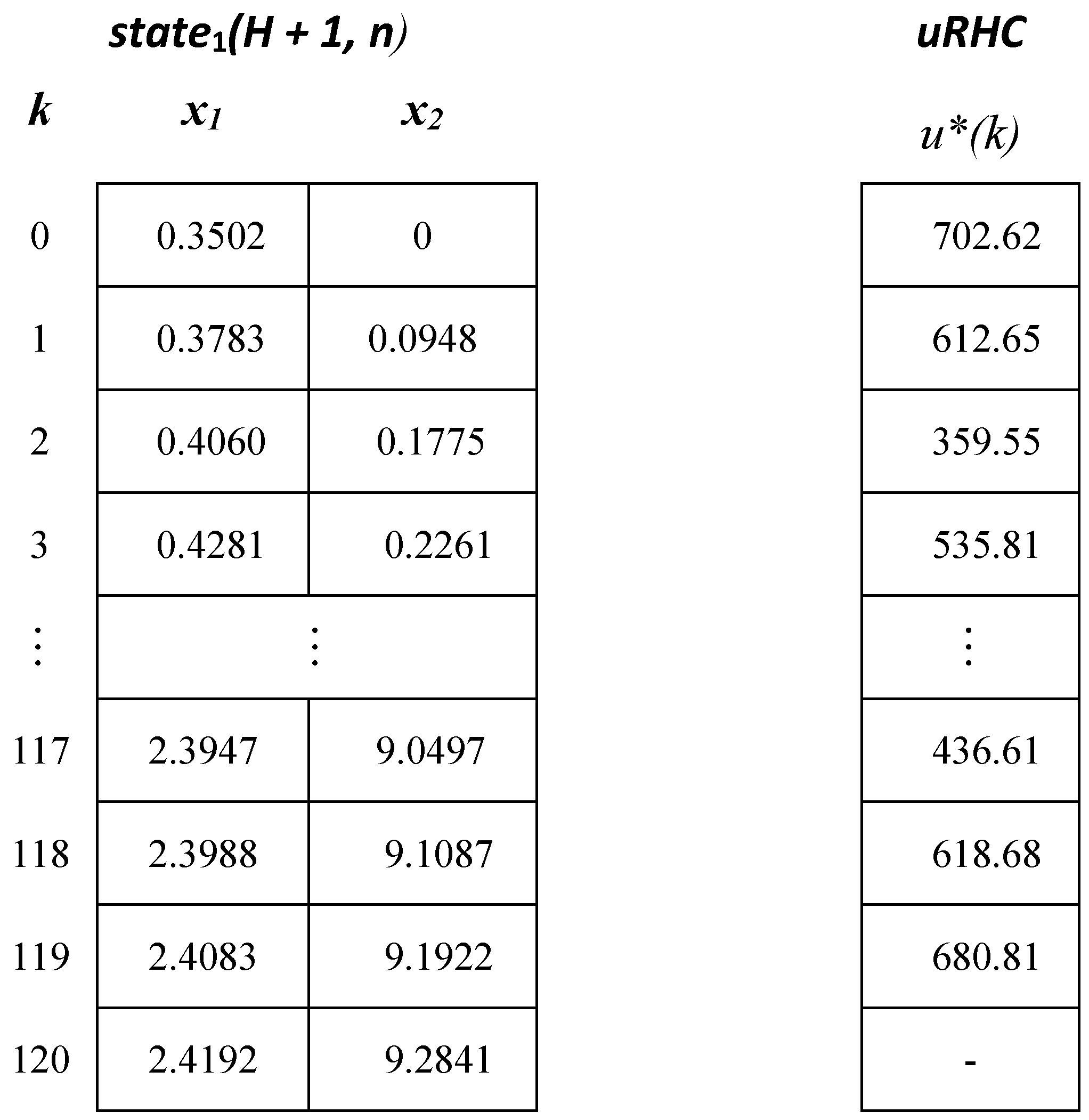
The optimal control value and the optimal states are stored in the matrices uRHC (H × m) and state (H + 1 × n), respectively, having the structure presented in Figure 4.
Hence, the optimal CP and trajectory are described by the matrix uRHC and state, respectively, which are the images of and sequences (see (5) and (6)). For each of the M simulations, the two matrices are saved in the cell array STATE and the matrix UstarRHC (M × H), as suggested in Figure 5 for our case study.
- □
- The script LOOP_M_ControlLoop_PSO.m collects the data from M executions of the closed-loop simulation. The data structures presented in Figure 5 are created and loaded. A concrete example of data collected in the first simulation is given in Appendix B.
4. The ML Controller. The Design Procedure and the General Algorithm
The M simulations can be collectively presented in Figure 6, where the state variables and control output are regrouped by sampling periods.
At each step of the control horizon, the controller predicts the optimal control output relaying on the couple (APSOA, PM). The state vectors considered at the same step have some common characteristics:
- The same PSO algorithm generates the M state inside a group.
- The M simulations work with the same PM.
- Each state is transferred as the initial state to the predictor.
- The prediction horizon has sampling periods.
The APSOA calculates the prediction , and the controller extracts only the optimal control values .
The simulation results for step k can be organized as a dataset, and a table can be constructed as below.
We have considered, as usual, that the state and control vector are column vectors. In our case study, the state vector (n=2) is generated like a ligne vector to avoid transposition.
When M has a big enough value, the dataset from Table 1 represents to some extent the ability of the couple (APSOA, PM) to predict optimal control values at step k. Our desideratum is to generalize this ability to predict the optimal control when the process accesses other states than those from Table 1; this can be done using a machine learning algorithm.
Remark 4.
The four characteristics enumerated before are the reasons making us adopt the hypothesis that the examples (data points) of Table 1 belong to the same data-generating process; that is, they are independently identically distributed.
For each group of states presented in Figure 6, equivalent to a table like Table 1, a regression function can be associated:
When these functions exist, they can be used successively within the controller to replace the predictor at each control step.
Remark 5.
The regression function models how the APSOA determines the optimal prediction at step k. The entire set of functions is the couple (APSOA–PM) machine-learning model. The behaviour of the PSO algorithm, which, in turn, depends on the PM, is captured by the set of functions .
To be systematic, at this point of our presentation, we propose a design procedure for the ML controller that the interested reader could use in their implementation.
- Design procedure
- Write the “ControlLoop_PSO” program simulating the closed-loop working of the controller based on the PSO algorithm over the control horizon. The output data are the quasi-optimal trajectory and its associated control profile ( and ).
- Repeat M times the “ControlLoop_PSO” program’s execution to produce the sequences (, ) and save them in data structures similar to those in Figure 5.
- For each sampling period k, derive datasets similar to Table 1 from data saved at step 2.
- Determine the set of functions using the data sets derived at step 3 and an ML model; a function is associated with each sampling period k.
- Implement the new controller based on the ML model, i.e. the set of functions determined in step 4.
- Write the “CONTROL_loop” program to simulate the closed-loop functioning equipped with the ML controller. The proposed method’s feasibility, performance index, solution quality, and execution time will be evaluated.
Remark 6.
The entire design procedure of the ML controller needs only simulations and offline program executions. The ML models for each sampling period are determined offline ahead of using the ML controller in real time.
Steps 1-2 are already covered by the details given in the anterior Section.
Step 3 Implementation
This step yields the data sets that the ML model would use for training and testing.
Remark 7.
The controller’s optimal behaviour is specific to each sampling period whose prediction horizon is specific . So, optimal behaviour learning will be done for each sampling period.
For each k, we construct a matrix SOCSK (SOCSK stands for “States and Optimal Control values concerning Step K”), which is the Table 1’s image. Line i, , is devoted to experience i:
Using the data structures proposed before, it holds:
STATEi is the ith element of the STATE cell array. In the PBR case (n=2, m=1), the data set for the current step will be:
- □
- A fragment of the SOCSK matrix produced by a MATLAB script is presented in Appendix C for step k=1. Only when k=0 the value of x2(0) equals 0 for any observation.
Owing to Remark 7, step 3 should establish for each k the data sets for training and testing; these sets are stored in the cell arrays DATAKTest and DATAKTrain. Table 2 presents the pseudocode of the script preparing all the sets needed by the learning algorithm.
Step 4’s implementation will determine the set of ML models and will be treated in the next Section.
Step 5 aims to implement the ML controller. Once the set of regression models is determined in step 4, the controller can be written following the algorithm in Table 3.
Notice that the cumulative effect of calling the controller at each sampling period is to achieve the following sequence of predictions using the regression models and the current states the process accesses:
In the sequel, the controllers based on ML models will be called LR Controller (from Linear Regression) or RNN Controller (from Regression Neural Network).
5. Linear Regression Controller
5.1. General Algorithm
The first approach the authors considered was to use multiple linear regression for the functions set . Such a model contains an intercept, linear terms for each state variable, squared terms, products of features (interactions), etc. Hence, as functions of state variables, the regression functions could be nonlinear.
For our example, the stepwise regression strategy [30], which adds or removes terms starting from a constant model, was also applied. We consider in this presentation only models having an intercept, linear terms, and an interaction:
Remark 8
: Our goal is not to find the best sequence of linear regression models but to validate our approach, i.e. the ML model can successfully replace the couple (APSOA, PM) inside a new controller.
As we shall see, the models (7) are largely sufficient for our goal. Table 4 presents the construction of the H models representing linear regressions in a general manner, that is, not only for our example. This pseudocode describes the linear models’ training and testing using the sets generated in step 3.
The script in Table 4 uses the generic functions fitting_to_data, get_the_coefficients, and fpredict, which makes actions suggested by the comments.
- □
- The implementation of this algorithm is included in the script GENERATE_ModelSW; some details are given in Appendix D.
5.2. Simulation Results
Although we have determined the usual linear regressions that contain the two linear terms (for and ) and an intercept, we present hereafter the stepwise version as it is implemented in the MATLAB system. Table 5 displays a listing’s fragment obtained during the script GENERATE_ModelSW’s execution; this one presents the model for a single sampling period.
The procedure begins with only an intercept, and after that, it tries and succeeds in adding the term corresponding to . Statistic parameters do not allow adding of another term. So, the prediction (control value) will be .
We notice that the training time for all 120 linear regressions is 6.166654 seconds.
Following the algorithm presented before, the resulting coefficients of the H regression are given in Table 6.
There are sampling periods for which the regression model has only the intercept C0; this situation will be discussed in Section 7. These coefficients will be used directly by the controller as a control law.
The comparison achieved in lines #9-10 of the construction algorithm is summarised in Figure 7.
We have to mention that the predicted values were calculated directly using the formulas, not using the generic function fpredict. The table datakTest supplied the 60 examples, states - control value, for testing the linear regressions.
The quality of the predictions will be evaluated at the time of using the regression models within the controller, that is, inside the closed-loop simulation. The ultimate evaluation of predictions would be the optimality of the process evolution.
To prepare this evaluation, we need the simulation program for the control loop working with the LR controller. The flowchart in Figure 8 describes this program, CONTROL_loopLINREG, which is step #6 of the design procedure.
Although there are similarities with Figure 3, actually there are big differences in execution:
- The state variable has two elements.
- The coefficients’ matrix must be loaded from an existing file.
- The grey instructions make the predictions, avoiding any numerical integration.
- The green instruction updates the next state, which has two components. The amount of light irradiated in the current sampling period is added to x2(k).
Only the orange column of the flowchart has big similarities because it is about the simulation results needed to depict the process evolution and the performance index.
- □
- The script CONTROL_loopLINREG.m included in the attached folder implements the presented algorithm.
The closed-loop simulation program produces a listing, a fragment of which is presented in Table 7, and two drawings reproduced in Section 7. At every step, k, the current state, the predicted control value uML, and the process’s next state are displayed.
The final lines display the biomass produced, g, and the performance index J= 9.5981. We notice the very short while used to control the process over the entire control horizon, 0.6401 seconds (The simulation processor is Intel(R) Core(TM) i7-6700HQ CPU @ 2.60GHz).
6. Controller Based on Regression Neural Networks
6.1. General Approach
Because the linear regression could seem much too simple, we have studied other types of models trying to improve capturing the optimality of the couple (APSOA, PM), the final target being that the designed ML controller would approach better the optimal behaviour.
Better predictions than those obtained with other types of ML models are produced by Regression Neural Networks (RNNs), of course, with a possible penalty concerning the model’s size. The decision to choose between these models and the linear regressions in implementing the controller will be analyzed in Section 7.
As in the case of linear regressions, the RNN models must be obtained offline, and their construction must be organized in a loop because the number of sampling periods could be large, like in our case. The pseudocode of RNNs’ construction is presented in Table 8.
In our case study, for k=0, i.e. the first sampling period, we have a special situation because (the light amount equals 0 by initialization) for all examples. Hence, this variable can not be a prediction variable. For this situation, the tables datakTrain and datakTest have different structures, and the RNN model has a single predictor variable . To keep a general structure of the algorithm in Table 8, we did not treat the first sampling period distinctly.
Most data structures were presented before except the cell array MODELNN that collects the model for each sampling period, called “mdlNN”. The function trainRegNN trains the current RNN using its specific dataset [20].
In line #6, the predictions made by the method “mdlNN.predictFcn” are stored in the local table predictionNN, which can be compared to datakTest or saved for further utilization.
- □
- The implementation of this algorithm is achieved by the script GENERATE_ModelNN; some details are given in Appendix E.
6.2. Simulation Results
The execution of the script GENERATE_ModelNN gives us an indication of RNNs’ construction complexity (training and testing). A fragment of its listing is given in Table 9.
The RMSEValid is the Root Mean Square Error (RMSE) between the predictions and datakTest vectors. The vrmse value is the RMSE calculated in the training process (phase of validation). The program displays the k value, prediction uNNn, and the control value (valreal) for the states included in record #10 of the dataset (as an example).
We notice that all 120 RNNs are trained in 233 seconds (offline, as we mentioned before).
The comparison mentioned in line #7 of the algorithm can be achieved by calculating the root mean square error (RMSE) between predicted and observed values. For graphical analysis, Figure 9 plots the predicted values yielded by the RNN model versus the real control values from the datakTest table.
As in Section 5.2, to evaluate the controller’s performances, we need the simulation program for the closed-loop working with the RNN models. Its algorithm’s flowchart would be very similar to that of Figure 8, except for two instructions. That is why we do not redraw the flowchart, but we are content with indicating only the changes.
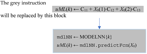 |
This block means that the neural network model mdlNN is selected as the current RNN from the cell array of objects MODELNN. Its method predictFcn will calculate the predicted control value as a function of the current state.
The second change is inside the block “Initializations”. Instead of loading the coefficients’ table, C, it will load the cell array MODELNN; the latter is already saved in a file created by the script constructing the RNN models (see GENERATE_ModelNN.m).
- □
- The script CONTROL_loopNN.m included in the attached folder implements the above algorithm.
The simulation program CONTROL_loopNN produces a listing, a fragment of which is presented in Table 10, and two drawings, presented in Section 6. At every step, the current state, the predicted control value uML, and the process’s next state are displayed.
The final lines display the biomass produced, g, and the performance index J= 9.5604. We notice, as in the case of the Linear Regression Controller, the very short while used to control the process over the entire control horizon, 1.35 seconds.
7. Discussion
7.1. Comparison between the PSO and ML Predictors
In this Section, we have to answer the following questions:
- Did the ML predictors succeed in “learning” the behaviour of the couple (APSOA, PM) such that the process’s evolution would be quasi-optimal?
- Did the controller’s execution time decrease significantly?
As we mentioned, we have already solved the PBR problem using RHC and a predictor based on PSO. For the sake of simplicity, we shall refer to its controller as the PSO Controller. Using the ControlLoop_PSO script, the closed-loop simulation produces the typical evolution depicted in Figure 10. This simulation is one among the M=200 evolutions that contributed to our big dataset with CPs and trajectories. The final lines of the simulation’s listing summarize its performances given in Table 11.
The simulation programs CONTROL_loopLINREG and CONTROL_loopNN produce, besides data in Table 7 and Table 10, the evolutions depicted in Figure 11 and Figure 12, respectively.
Remark 9.
The state evolutions ( and ) and the evolution of the biomass, which can be considered as the output of the process, are practically identical. Hence, both ML controllers emulate the PSO Controller.
The LR Controller and the RNN Controller are facing situations when the current state is totally new (states unobserved in the training or testing data sets). In this situation, the generalization ability of the ML model is exploited but also verified. That is why the simulation programs are adequate tests for the predictions’ testing.
Remark 10.
Using the controller inside a closed-loop simulation program over the control horizon will be a test in which the predictor experiences new process states unobserved in the training and testing phase of the ML model’s construction.
The fact that Figure 10a, Figure 11a and Figure 12a, describing the control value’s evolution, are very different has no relevance to the matter at hand; the following aspects uphold this:
- The similarity at this level would imply the same sequences of states, but we just stated that the ML controllers could experience new unobserved states. So, the three processes do not pass through the same set of states (the sets of accessible states are different).
- The learning is made at the level of each sampling period and “learns” couples (state, control value), not globally to the control profile level; our method is not based on learning CPs. On the other hand, the PSO predictor is very “noisy” due to its stochastic character and produces outliers among the 200 control values from time to time.
To make a quantitative comparison among the three controllers, Table 12 gathered some pieces of information from Table 7, Table 10 and Table 11.
The first four lines of Table 12 are evidence that the three controllers can be considered equally performant, although the ML controllers have slightly better parameters. However, the time devoted to controlling the process over the control horizon (all the H sampling period) has values much inferior to that of the PSO Controller (hundreds of times smaller). This analysis and Remark 9 allow us to state the following conclusions:
- (1) The two ML Controllers have predictors that have learned the behaviour of the couple (APSOA, PM) such that, in closed-loop working, the process evolves almost identically.
- (2) The resulting controllers have execution times hundreds of times smaller than that of the PSO Controller.
7.2. Comparison between the LR and RNN Controllers
In Table 12, all the parameters in the second column are superior to those in the third column. The differences are not relevant for some of them, but the control time, training time and model size make the LR Controller preferable to the RNN controller. However, we have trained all its RNNs using hyperparameter optimization.
The usual comparison between the predicted and real (observed) values is illustrated in Figure 7 and Figure 9 for the LR and RNN predictors, respectively. This comparison is made for k=10 (as an example) and its testing table datakTest. For the other values of k, the situation is the same.
At first sight, both predictors seem to be similar, but the values of RMSEs from Table 12 show that the LR predictor is slightly better than the RNN predictor. This remark goes in the same direction that states the superiority of the LR Controller. However, because the tatakTest has 60 data points, we can consider the difference between RMSEs irrelevant and that they are similar from the accuracy point of view.
Considering Remark 6, the time to train offline 120 RNNs (for the RNN Controller) in 4 minutes is absolutely acceptable. So, even this controller can be considered a good solution for the PBR problem or another OCP.
For the reader, who is a newcomer conjointly in the fields of control systems, computational intelligence, and machine learning, we must compare the role of the PSO predictor versus the role of the ML predictor when solving an OCP.
- The PSO predictor predicts an optimal control value, but first, it searches for the optimal value following its optimization mechanism using a swarm of particles and the PM. That is why it takes a “long” time to find this value after a convergence process.
- The ML predictor (LR or RNN) predicts using an already-known regression function. Being an ML model, it reproduces what it has learned, the PSO predictor’s behaviour. It does not search for anything. Moreover it does not make numerical integrations of the PM. That is why it takes a “short” time to calculate the predicted value.
- The ML predictor replaces the PSO predictor only in execution when the controller achieves the control action. So, the controller’s execution time is hundreds of times smaller than initially. That was our desideratum.
- When we solve a new OCP, sometimes we need a metaheuristic (PSO, EA, etc) that searches for the optimal solution inside of a control structure. If the controller’s execution time is not acceptable, we can use the approach presented in this paper to create an ML controller. However, initially, we need something to search for the optimal solution.
8. Conclusions
In this paper, we have proposed two ML controllers (LR Controller and RNN Controller), including the Linear Regression and Regression Neural Network predictors, that can replace the controller using a PSO algorithm; the optimal control structure works with an internal process model.
The machine learning models succeeded in “learning” the quasi-optimal behaviour of the couple (PSO, PM) using data capturing the PSO predictor’s behaviour. The training data is the optimal control profiles and trajectories recorded during M offline simulations of the closed-loop over the control horizon.
The paper proposes algorithms for collecting data and aggregating data sets for the learning process. The learning process is split to the level of each sampling period so that a predictor model is trained for each one. The multiple Linear Regression and the Regression Neural Networks were considered as predicting models.
For each case, we proposed algorithms for constructing the set of ML models and the controller (LR or RNN Controller). Algorithms for the closed-loop simulations using the two controllers are also proposed; they allow us to compare the process evolutions involved by the three controllers, PSO, LR, and RNN Controller.
The final simulations showed that the new controllers preserved the quasi-optimality of the process evolution. In the same conditions, the process evolutions were almost identical.
An advantage of our approach refers to the data collecting, data sets’ preparation for the training process, and the construction of ML models; all these activities need only simulations (using PSO Controller) and offline program executions (Remark 6). The ML models for each sampling period are determined offline ahead of using the ML controller in real-time.
We emphasize that, during the final closed-loop simulations, the ML controller encounters new process states unobserved in the training and testing of its predictor (Remark 10). Owing to its generalization ability, the controller makes accurate predictions of the control value sent to the process.
The PSO predictor first searches for the optimal control value, following its optimization mechanism using particles and the PM, before predicting it. This search sometimes means a big computational effort and a large controller’s execution time. The ML controller (LR or RNN) predicts using an already-known regression function, which can emulate the PSO predictor. In other words, the ML predictor replaces the PSO predictor only in execution when the controller achieves the control action. That is why the controller’s execution time decreases drastically. However, the solution belongs intrinsically to the PSO predictor.
When we solve a new OCP, sometimes, for different reasons, we shall need a metaheuristic (PSO, EA, etc) searching for the optimal solution, inside of a control structure. Finally, the implemented controller integrated into the control structure can be one of the two ML controllers.
In our opinion, this work goes beyond the controller’s execution time decrease and opens a perspective to emulate and replace in a general manner optimization structures.
Supplementary Materials
The following supporting information can be downloaded at the website of this paper posted on Preprints.org. The archive “ART_Math.zip” contains the files mentioned in Appendixes A, B, C, D and E.
Author Contributions
Conceptualization, V.M.; methodology, V.M.; software, V.M. and I.A.; validation, V.M. and E.R.; formal analysis, V.M.; investigation, I.A.; resources, E.R.; data curation, I.A.; writing—original draft preparation, V.M.; writing—review and editing, V.M. and E.R.; visualization, E.R; supervision, I.A.; project administration, I.A.; funding acquisition, E.R. All authors have read and agreed to the published version of the manuscript.
Funding
This research was funded by the Executive Agency for Higher Education, Research, Development and Innovation Funding (UEFISCDI - Roumania), project code COFUND-LEAP-RE-D3T4H2S; Europe Horizon – LEAP-RE program. The APC received no external funding.
Data Availability Statement
Not applicable.
Acknowledgments
This work benefited from the administrative support of the Doctoral School of “Dunarea de Jos” University of Galati, Romania.
Conflicts of Interest
The authors declare no conflicts of interest.
Appendix A
The controlled physical system is a flat-plate photobioreactor (PBR) lighted on a single side for algae growth. The constructive and physical parameters are presented in Table A1. Their definitions are irrelevant to this work.
The PBR is a distributed parameter system because the light is attenuated inside. To convert it into a lumped-parameter system, its depth, L=0.04 m, is discretized in points equally spaced (. After discretization, the process model (PM) is as follows:
The control input u(t) is considered to be the intensity of incident light:
u(t) = q(t)
The state variables are the following:
: the biomass concentration (in g·/L);
: the light amount which, up to moment t, has illuminated the PBR (in µmol/m2/s).

Table A1.
The constants of the PBR model.
| = 172 m2·kg−1 | absorption coefficient |
| = 870 m2·kg−1 | scattering coefficient |
| = 0.0008 | backward scattering fraction |
| = 0.16 h−1 | specific growth rate |
| = 0.013 h−1 | specific decay rate |
| = 120 µmol·m−2·s−1 | saturation constant |
| = 2500 µmol·m−2·s−1 | inhibition constant |
| = 1.45·10−3 m3 | the volume of the PBR |
| L = 0.04 m | depth of the PBR |
| A = 3.75·10−2 m2 | lighted surface |
| = 0.36 g/L | the initial biomass concentration |
| C =3600·10−2 | light intensity conversion constant |
| =100 | number of discretization points |
| lower technological light intensity | |
| upper technological light intensity | |
| = 3 g. | the minimal final biomass |
| tfinal = 120 h | control horizon |
| T= 1 h | sampling period |
The output variable, the biomass m(t) calculated by equation (11), is the PBR’s product.
As a productivity constraint, it must hold
The cost function (A2) represents the amount of light used for the current batch while constraint (A1) is fulfilled. The two weight factors ( and ) are established by simulation.
Appendix B
Our implementations are based on the MATLAB system and language. The reader can find inside the folder Processes_PSO_ML, supplied in Supplementary Materials, the guide “READ ME.txt”. The following scripts can be used to carry out the closed-loop simulation:
- ControlLoop_PSO_RHC.m that implements the “ControlLoop_PSO” program;
- INV_PSO_Predictor1.m that implements the “Predictor_PSO” function;
- INV_RealProcessStep.m that implements the “ProcessStep” function.
The functions called recursively are also present inside the folder.
The script LOOP_M_ControlLoop_PSO.m also included in Supplementary Materials, gathers data from all the 200 simulations and saves them in the file WS_data200.mat.
A fragment of matrices describing a closed-loop simulation’s data, that is, the quasi-optimal evolution, is given in Figure A1. Notice that we have a single control variable, and the 121st state is the final one.
Figure A1.
The matrices for the optimal trajectory and its CP (first simulation)
Appendix C
A fragment of the SOCSK matrix produced by a MATLAB script is presented hereafter:
Table A1.
The matrix SOCSK for the second sampling period (k=1).
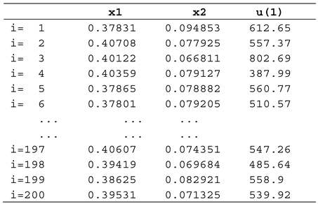
The matrices like this one, presented in Table A1, are the data sets that allow the construction of the ML models for each sampling period.
Appendix D
The linear regression models’ construction
This construction of the H=120 linear regressions is achieved by the script GENERATE_ModelSW. The latter opens the file WS_Modelsv1.mat (see below) to load the needed data sets.
The generic functions fitting_to_data and get_the_coefficients from Table 4 correspond to MATLAB functions stepwiselm and mdlsw.Coefficients.Estimate. The fpredict function is directly implemented using the regression formula and the coefficients.
The reader can also examine the script Model_ConstructionLINREG.m, which does not use the stepwise regression strategy; the regression models contain only the two linear terms and an intercept. The coefficients for all 120 regression functions are stored in the file WS_3coeff.mat. The cell arrays, MODEL -which stores the 120 objects of type linear regression-, DATAKTest, and DATAKTrain, are saved in the file WS_Modelsv1.mat.
Appendix E
The script GENERATE_ModelNN.m implements the algorithm presented in Table 7. We recall that it is carried out offline at step 5 of the design procedure.
The function trainRegNN is implemented in two versions by the scripts trainRegNNK0.m for the first sampling period and trainRegNN.m for the others; it trains the RNN and can be generated automatically using the Regression Application (eventually with hyperparameters optimization) or written ad-hoc using another training function. As an orientation, we give here a few RNN parameters:
RNN = fitrnet(predictors, response…,
‘LayerSizes’, [14 1 7], …
‘Activations’, ‘none’, …
‘Lambda’, 0.00015, …
‘IterationLimit’, 1000, …
‘Standardize’, true);
(see documentation [20]).
References
- Siarry, P. Metaheuristics; Springer: Berlin/Heidelberg, Germany, 2016; ISBN 978-3-319-45403-0. [Google Scholar]
- Talbi, E.G. Metaheuristics—From Design to Implementation; Wiley: Hoboken, NJ, USA, 2009; ISBN 978-0-470-27858-1. [Google Scholar]
- Kruse, R.; Borgelt, C.; Braune, C.; Mostaghim, S.; Steinbrecher, M. Computational Intelligence—A Methodological Introduction, 2nd ed.; Springer: Berlin/Heidelberg, Germany, 2016. [Google Scholar]
- Faber, R.; Jockenhövelb, T.; Tsatsaronis, G. Dynamic optimization with simulated annealing. Comput. Chem. Eng. 2005, 29, 273–290. [Google Scholar] [CrossRef]
- Onwubolu, G.; Babu, B.V. New Optimization Techniques in Engineering; Springer: Berlin/Heidelberg, Germany, 2004. [Google Scholar]
- Valadi, J.; Siarry, P. Applications of Metaheuristics in Process Engineering; Springer International Publishing: Berlin/Heidelberg, Germany, 2014; pp. 1–39. [Google Scholar] [CrossRef]
- Minzu, V.; Riahi, S.; Rusu, E. Optimal control of an ultraviolet water disinfection system. Appl. Sci. 2021, 11, 2638. [Google Scholar] [CrossRef]
- Minzu, V.; Ifrim, G.; Arama, I. Control of Microalgae Growth in Artificially Lighted Photobioreactors Using Metaheuristic-Based Predictions. Sensors 2021, 21, 8065. [Google Scholar] [CrossRef] [PubMed]
- Abraham, A.; Jain, L.; Goldberg, R. Evolutionary Multiobjective Optimization—Theoretical Advances and Applications; Springer: Berlin/Heidelberg, Germany, 2005; ISBN 1-85233-787-7. [Google Scholar]
- Hu, X.B.; Chen, W.H. Genetic algorithm based on receding horizon control for arrival sequencing and scheduling. Eng. Appl. Artif. Intell. 2005, 18, 633–642. [Google Scholar] [CrossRef]
- Mînzu, V.; Arama, I. A Machine Learning Algorithm That Experiences the Evolutionary Algorithm’s Predictions—An Application to Optimal Control. Mathematics 2024, 12, 187. [Google Scholar] [CrossRef]
- Mayne, D.Q.; Michalska, H. Receding Horizon Control of Nonlinear Systems. IEEE Trans. Autom. Control. 1990, 35, 814–824. [Google Scholar] [CrossRef]
- Mînzu, V.; Rusu, E.; Arama, I. Execution Time Decrease for Controllers Based on Adaptive Particle Swarm Optimization. Inventions 2023, 8, 9. [Google Scholar] [CrossRef]
- Goggos, V.; King, R. Evolutionary predictive control. Comput. Chem. Eng. 1996, 20 (Suppl. 2), S817–S822. [Google Scholar] [CrossRef]
- Chiang, P.-K.; Willems, P. Combine Evolutionary Optimization with Model Predictive Control in Real-time Flood Control of a River System. Water Resour. Manag. 2015, 29, 2527–2542. [Google Scholar] [CrossRef]
- Minzu, V.; Serbencu, A. Systematic procedure for optimal controller implementation using metaheuristic algorithms. Intell. Autom. Soft Comput. 2020, 26, 663–677. [Google Scholar] [CrossRef]
- Alatefi, S.; Abdel Azim, R.; Alkouh, A.; Hamada, G. Integration of Multiple Bayesian Optimized Machine Learning Techniques and Conventional Well Logs for Accurate Prediction of Porosity in Carbonate Reservoirs. Processes 2023, 11, 1339. [Google Scholar] [CrossRef]
- Guo, R.; Zhao, Z.; Huo, S.; Jin, Z.; Zhao, J.; Gao, D. Research on State Recognition and Failure Prediction of Axial Piston Pump Based on Performance Degradation Data. Processes 2020, 8, 609. [Google Scholar] [CrossRef]
- Minzu, V.; Riahi, S.; Rusu, E. Implementation aspects regarding closed-loop control systems using evolutionary algorithms. Inventions 2021, 6, 53. [Google Scholar] [CrossRef]
- The MathWorks Inc. (2024a). Regression Neural Network Toolbox Documentation, Natick, Massachusetts: The MathWorks Inc. Available online: https://www.mathworks.com/help/stats/regressionneuralnetwork.html.
- Minzu, V.; Georgescu, L.; Rusu, E. Predictions Based on Evolutionary Algorithms Using Predefined Control Profiles. Electronics 2022, 11, 1682. [Google Scholar] [CrossRef]
- Goodfellow, I.; Bengio, Y.; Courville, A. Machine Learning Basics. In Deep Learning; The MIT Press, USA, 2016; pp. 95–161; ISBN 978-0262035613.
- Zou, S.; Chu, C.; Shen, N.; Ren, J. Healthcare Cost Prediction Based on Hybrid Machine Learning Algorithms. Mathematics 2023, 11, 4778. [Google Scholar] [CrossRef]
- Cuadrado, D.; Valls, A.; Riaño, D. Predicting Intensive Care Unit Patients’ Discharge Date with a Hybrid Machine Learning Model That Combines Length of Stay and Days to Discharge. Mathematics 2023, 11, 4773. [Google Scholar] [CrossRef]
- Albahli, S.; Irtaza, A.; Nazir, T.; Mehmood, A.; Alkhalifah, A.; Albattah, W. A Machine Learning Method for Prediction of Stock Market Using Real-Time Twitter Data. Electronics 2022, 11, 3414. [Google Scholar] [CrossRef]
- Wilson, C.; Marchetti, F.; Di Carlo, M.; Riccardi, A.; Minisci, E. Classifying Intelligence in Machines: A Taxonomy of Intelligent Control. Robotics 2020, 9, 64. [Google Scholar] [CrossRef]
- Banga, J.R.; Balsa-Canto, E.; Moles, C.G.; Alonso, A. Dynamic optimization of bioprocesses: Efficient and robust numerical strategies. J. Biotechnol. 2005, 117, 407–419. [Google Scholar] [CrossRef] [PubMed]
- Balsa-Canto, E.; Banga, J.R.; Aloso, A.V.; Vassiliadis. Dynamic optimization of chemical and biochemical processes using restricted second-order information 2001. Comput. Chem. Eng. 2001, 25, 539–546. [Google Scholar]
- Newbold, P.; Carlson, W.L.; Thorne, B. Multiple Regression. In Statistics for Business and Economics, 6th ed.; Pfaltzgraff, M., Bradley, A., Eds.; Publisher: P ding x1, FStat = 12.7755, pearson Education, Inc: New Jersey, 07458, USA, 2007; pp. 454–537. [Google Scholar]
- The MathWorks Inc. (2024a). Stepwise Regression Toolbox Documentation, Natick, Massachusetts: The MathWorks Inc. Available online: https://www.mathworks.com/help/stats/stepwise-regression.html.
- Goodfellow, I.; Bengio, Y.; Courville, A. Example: Linear Regression. In Deep Learning; The MIT Press: USA, 2016; pp. 104–113. ISBN 978-0262035613. [Google Scholar]
Figure 1.
Receding Horizon Control Using Adaptive PSO Algorithm
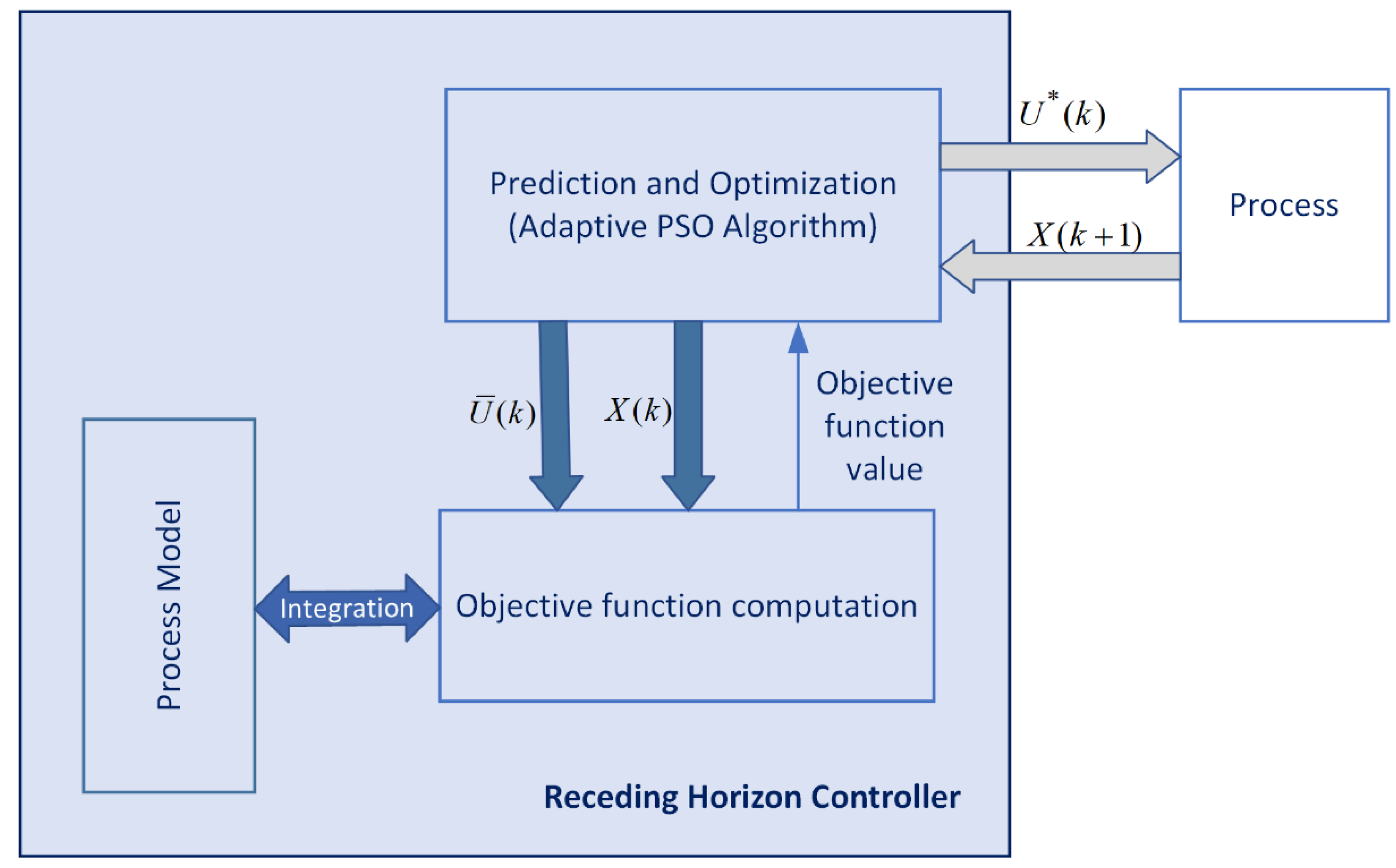
Figure 2.
The state trajectory and its CP.
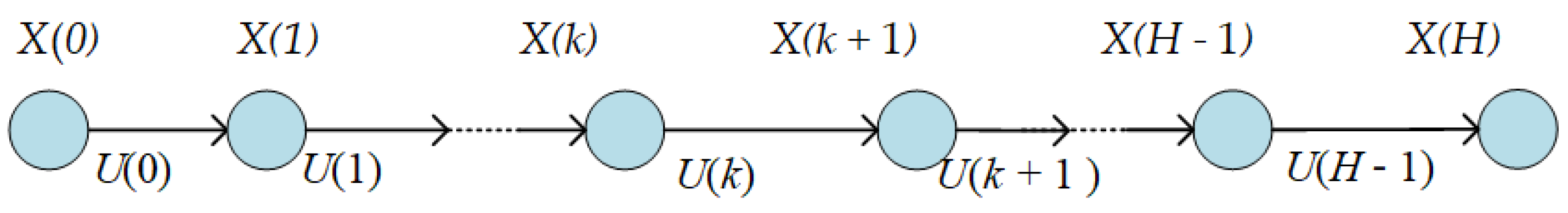
Figure 3.
Closed loop simulation using predictions based on adaptive PSO algorithm.
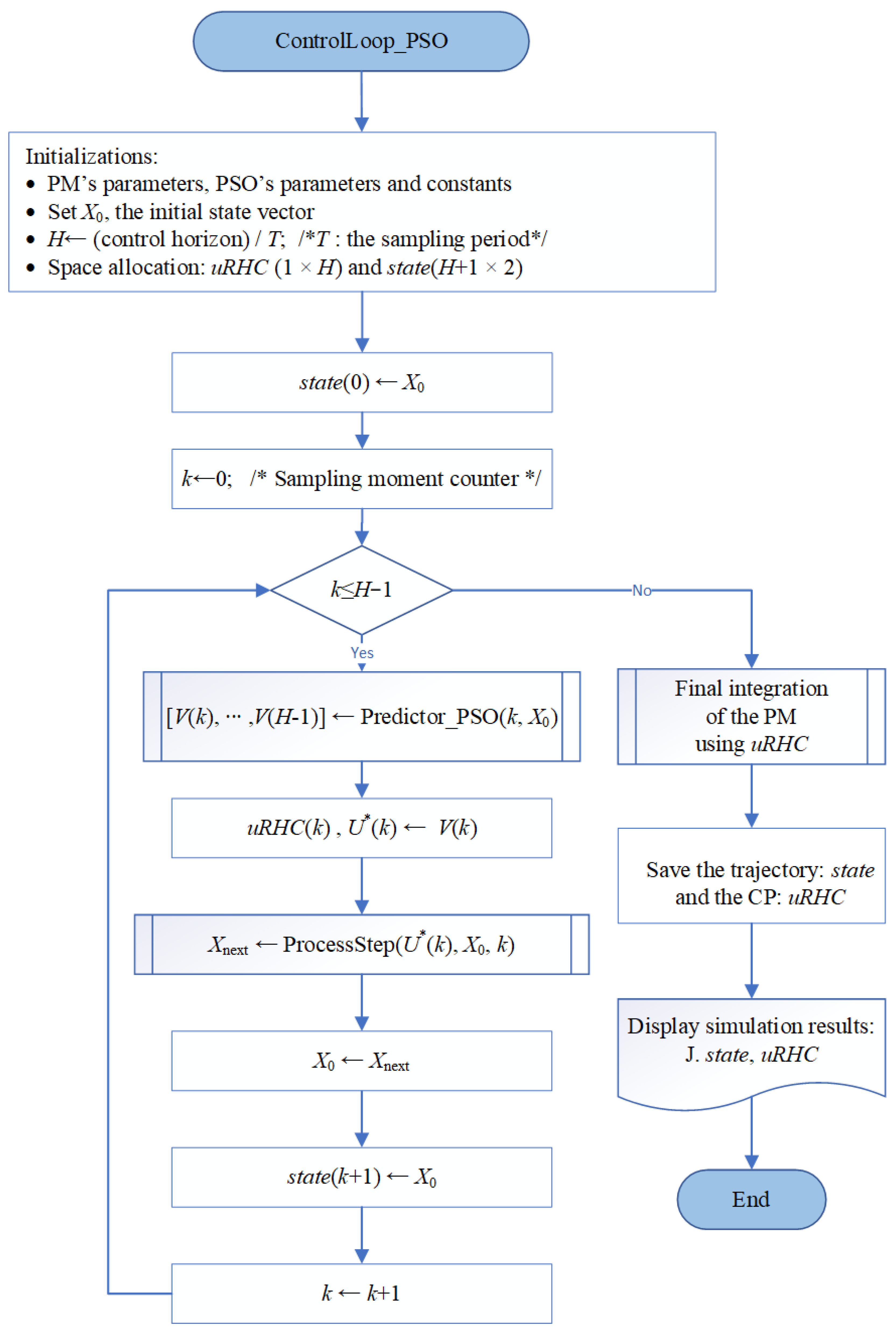
Figure 4.
The matrices that store the quasi-optimal trajectory and its CP.
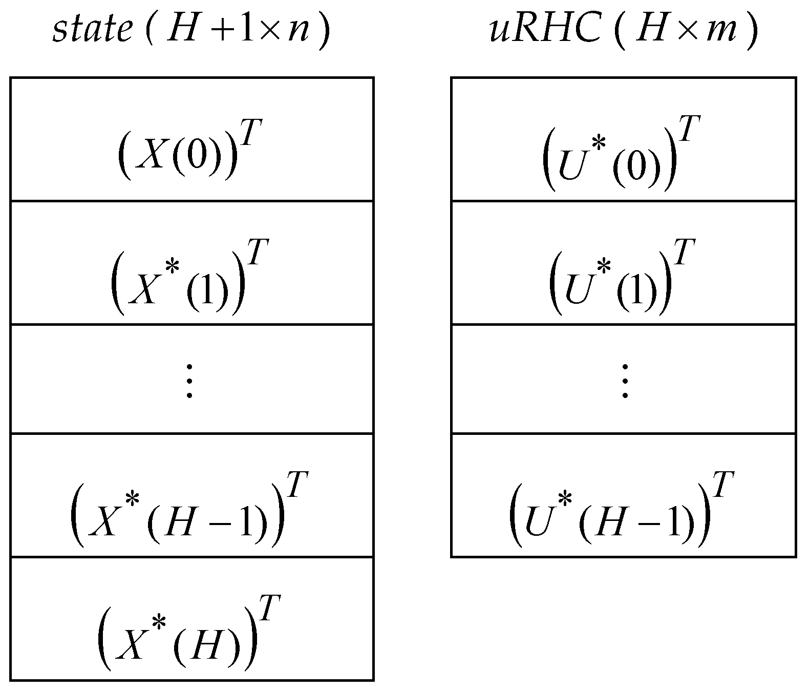
Figure 5.
The data collected following the M executions of the closed-loop simulation
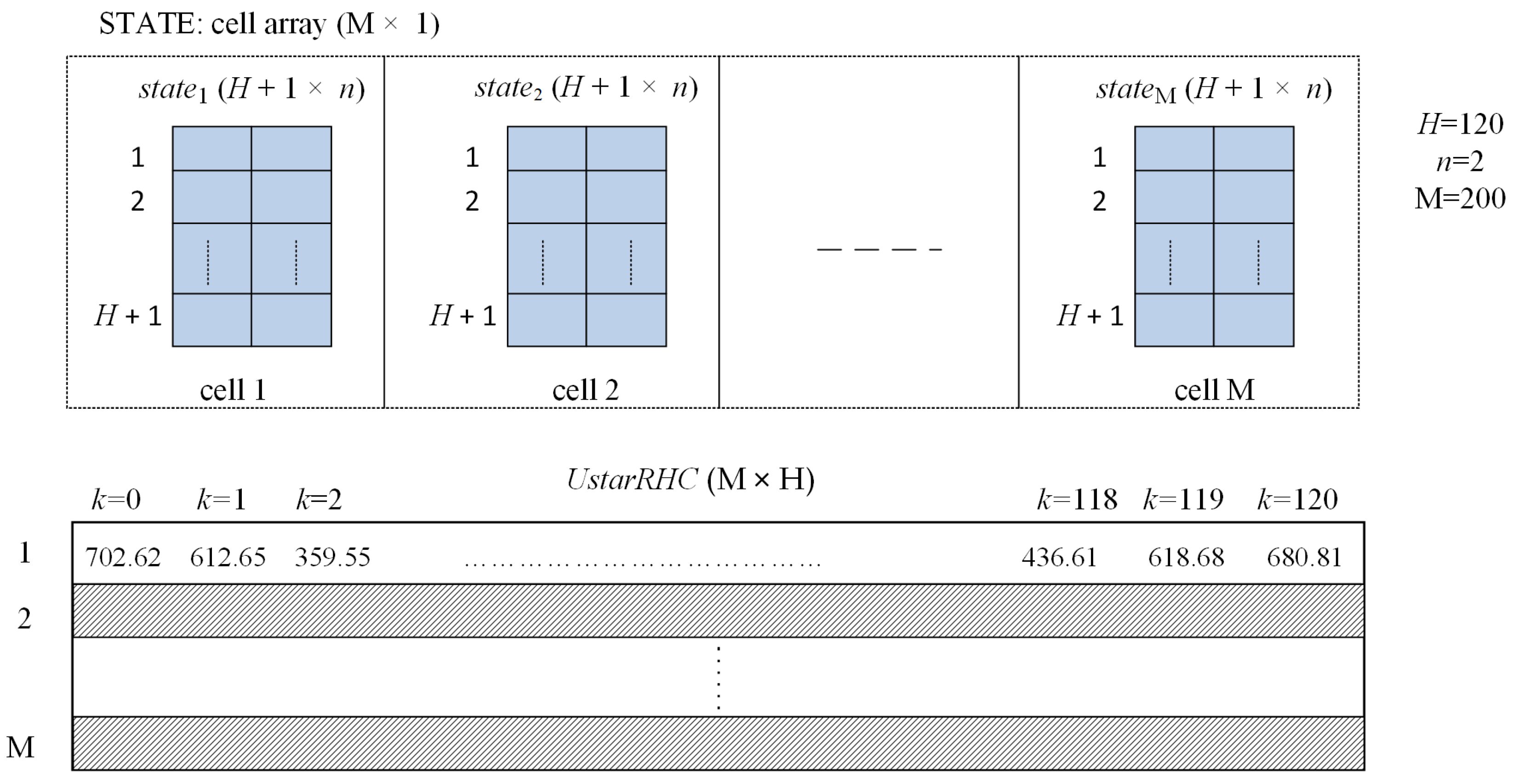
Figure 6.
The quasi-optimal trajectories produced by M execution of “ControlLoop_PSO.”
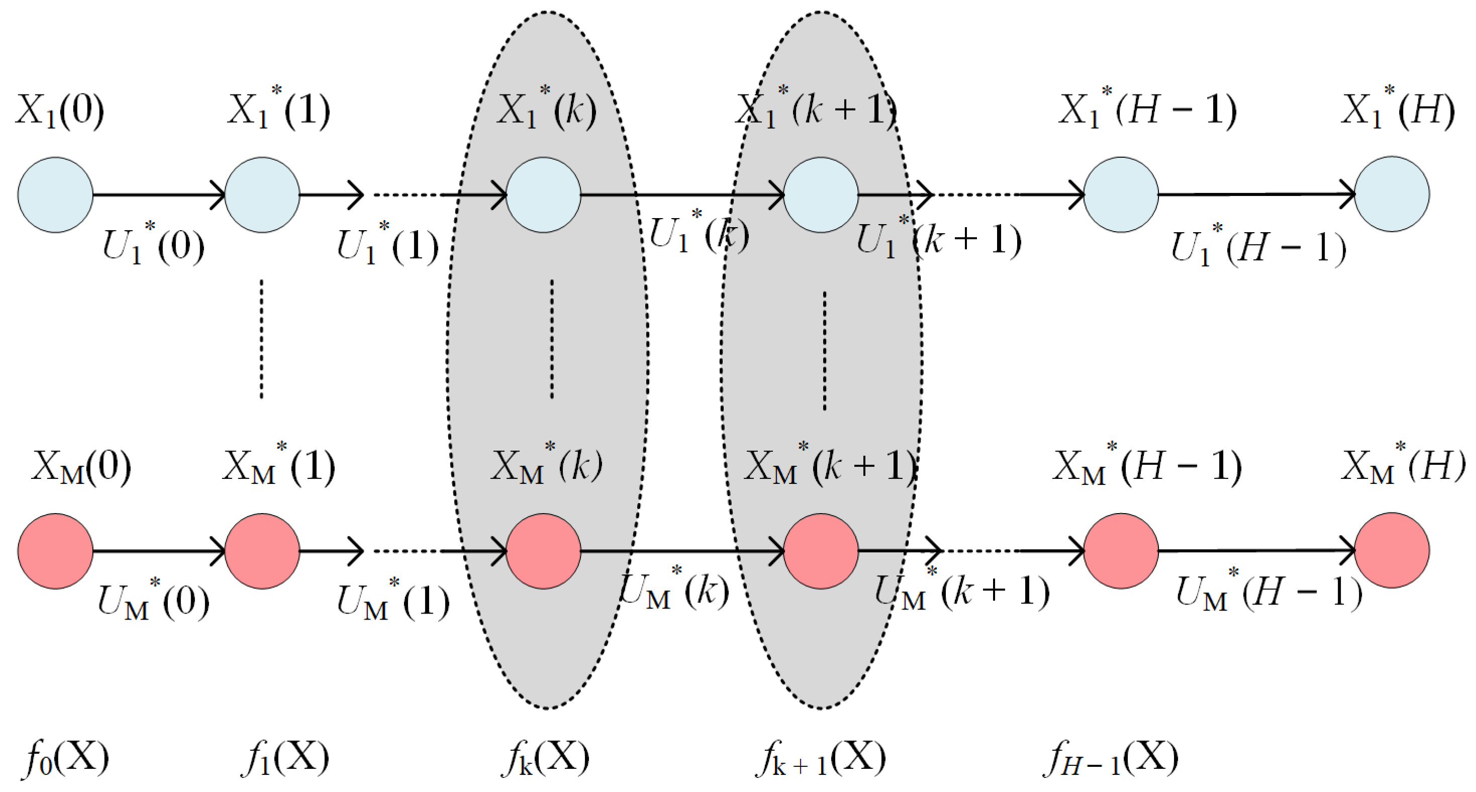
Figure 7.
Comparison: Predicted versus Real Control Values for a specific sampling period.
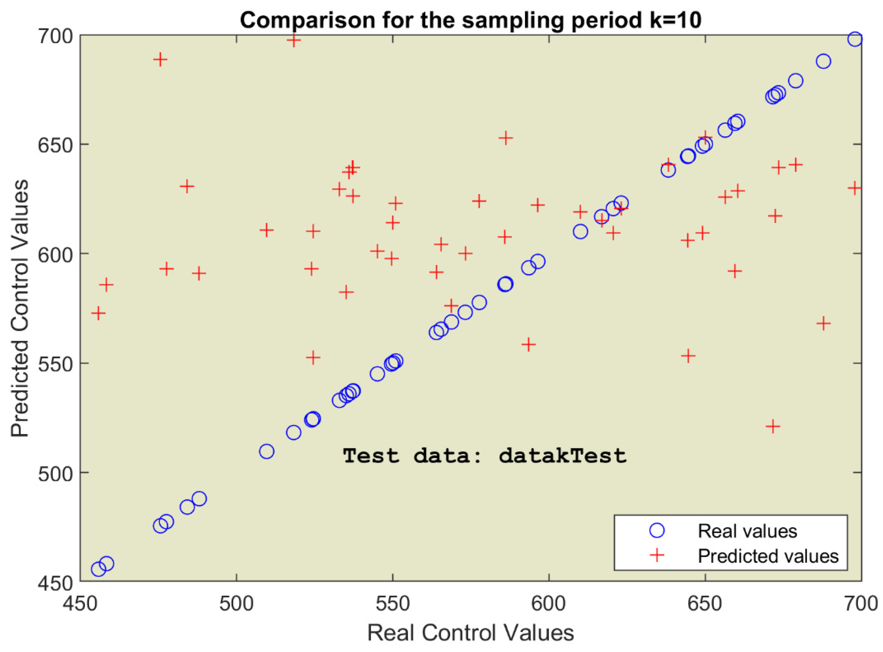
Figure 8.
The simulation program for the ML controller based on linear regression models.
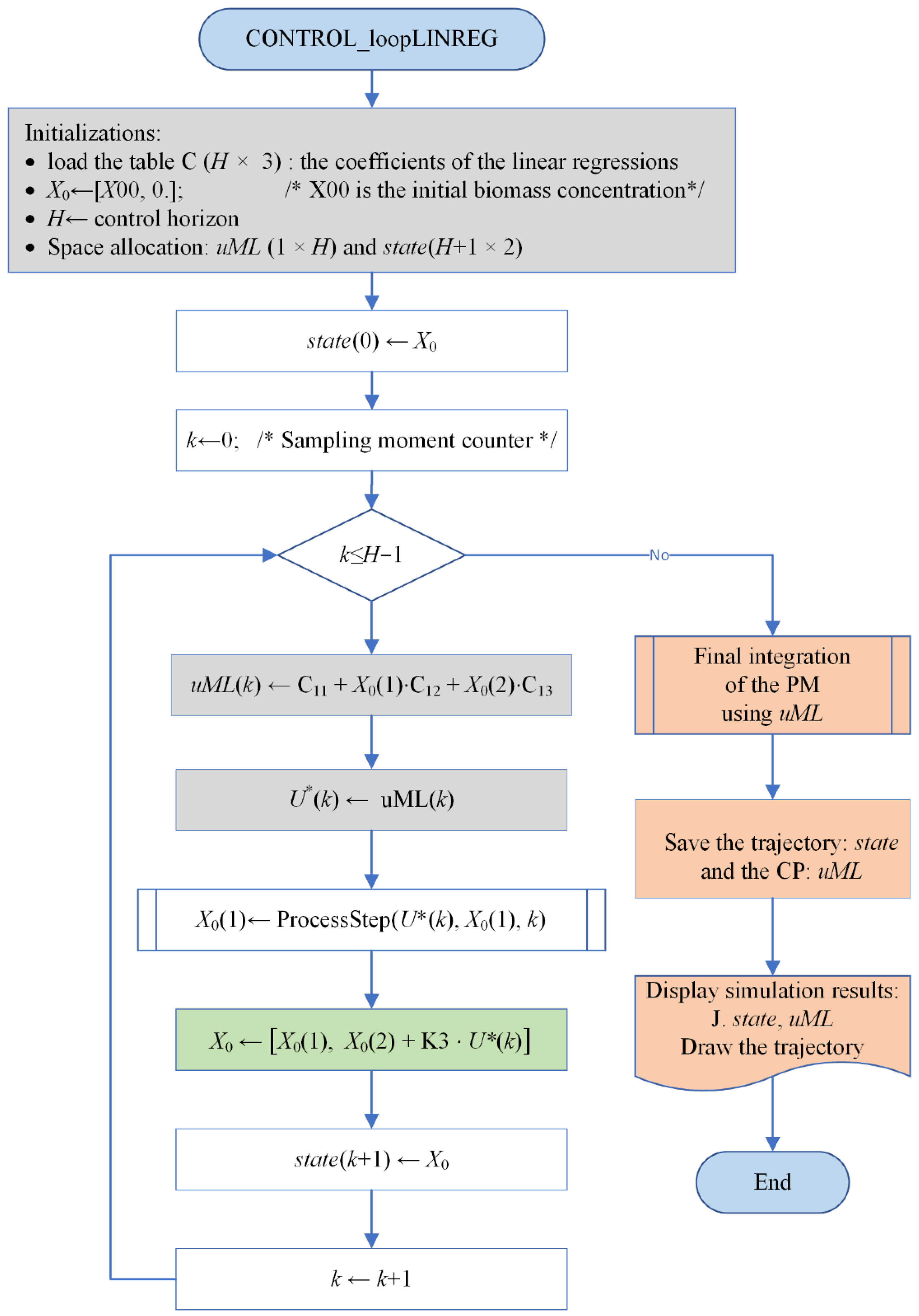
Figure 9.
Predicted values yielded by the RNN model versus Real Control Values for a specific sampling period.
Figure 9.
Predicted values yielded by the RNN model versus Real Control Values for a specific sampling period.
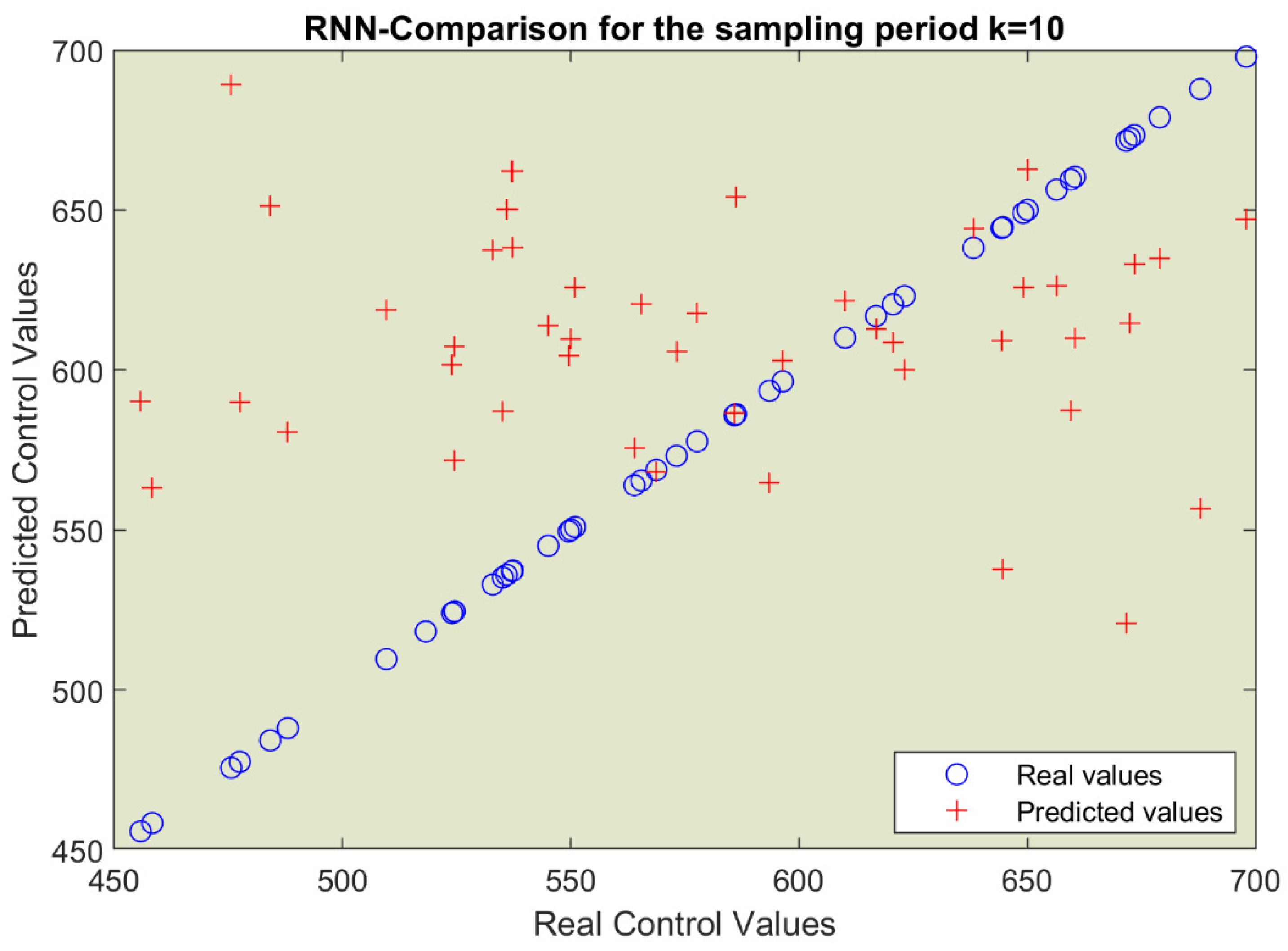
Figure 10.
Closed-loop evolution with PSO Controller. (a) The control output values over the control horizon; (b) The process and the biomass evolution.
Figure 10.
Closed-loop evolution with PSO Controller. (a) The control output values over the control horizon; (b) The process and the biomass evolution.
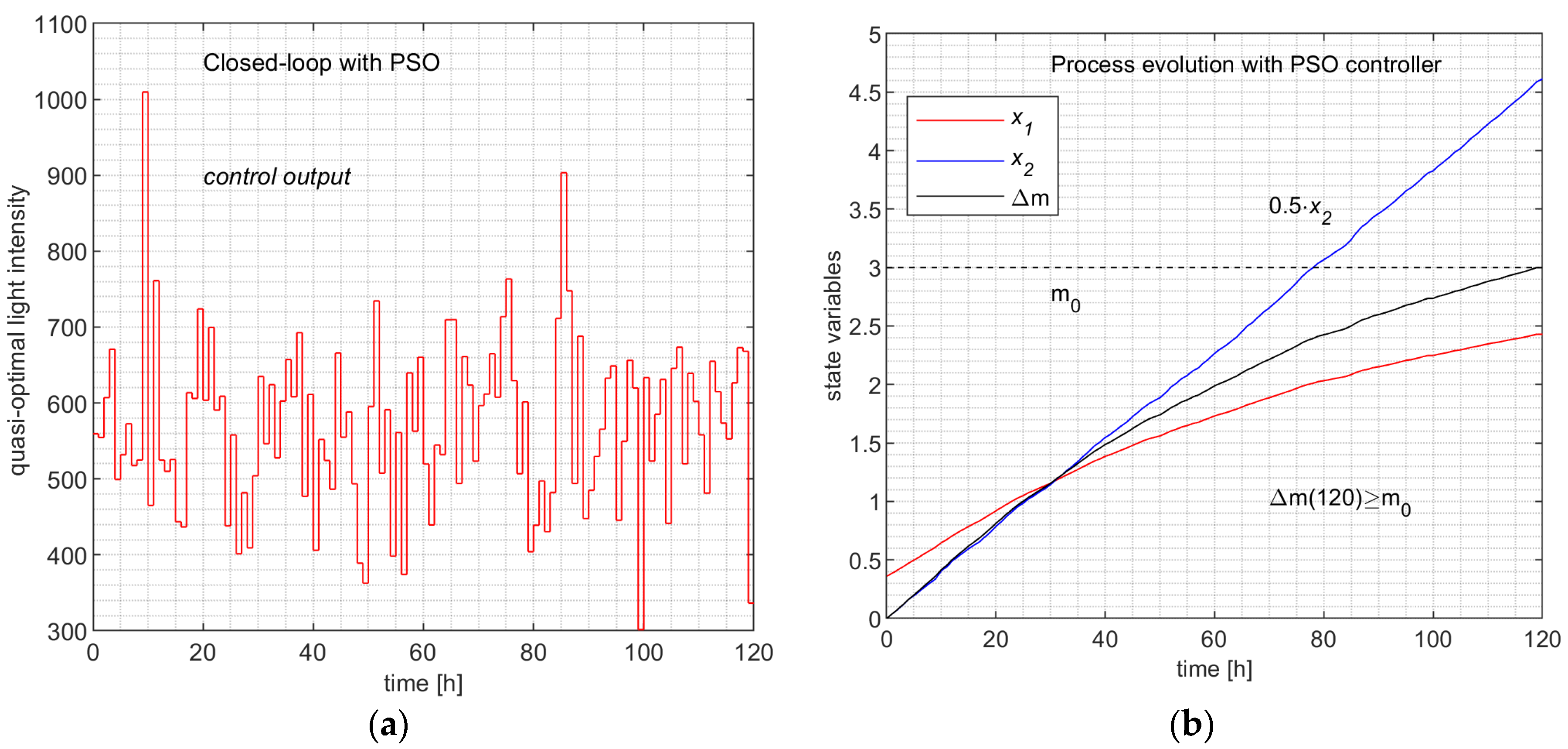
Figure 11.
Closed-loop evolution with Linear Regression Controller. (a) The control output values over the control horizon; (b) The process and the biomass evolution.
Figure 11.
Closed-loop evolution with Linear Regression Controller. (a) The control output values over the control horizon; (b) The process and the biomass evolution.
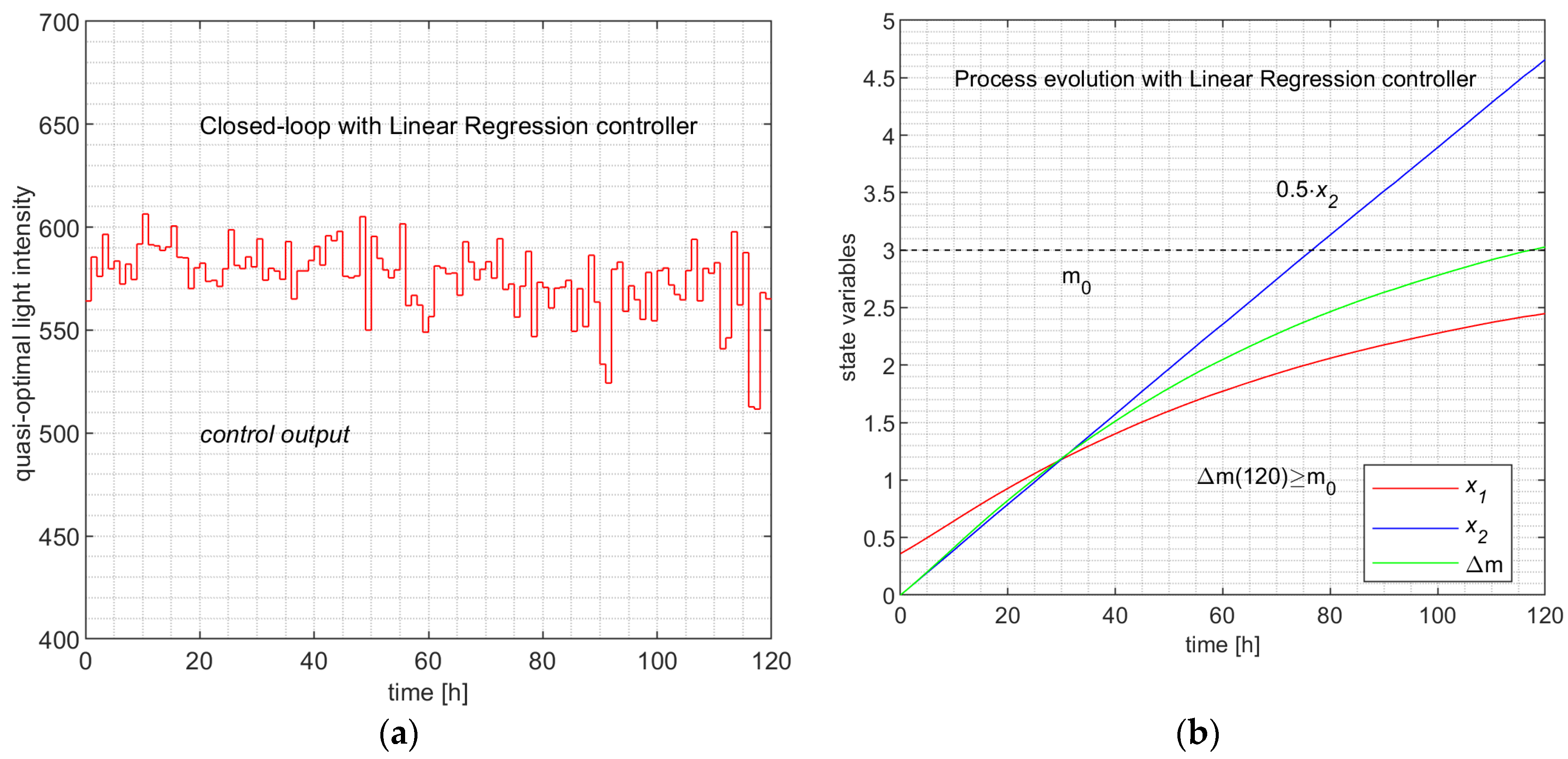
Figure 12.
Closed-loop evolution with Regression Neural Network Controller. (a) The control output values over the control horizon; (b) The process and the biomass evolution.
Figure 12.
Closed-loop evolution with Regression Neural Network Controller. (a) The control output values over the control horizon; (b) The process and the biomass evolution.
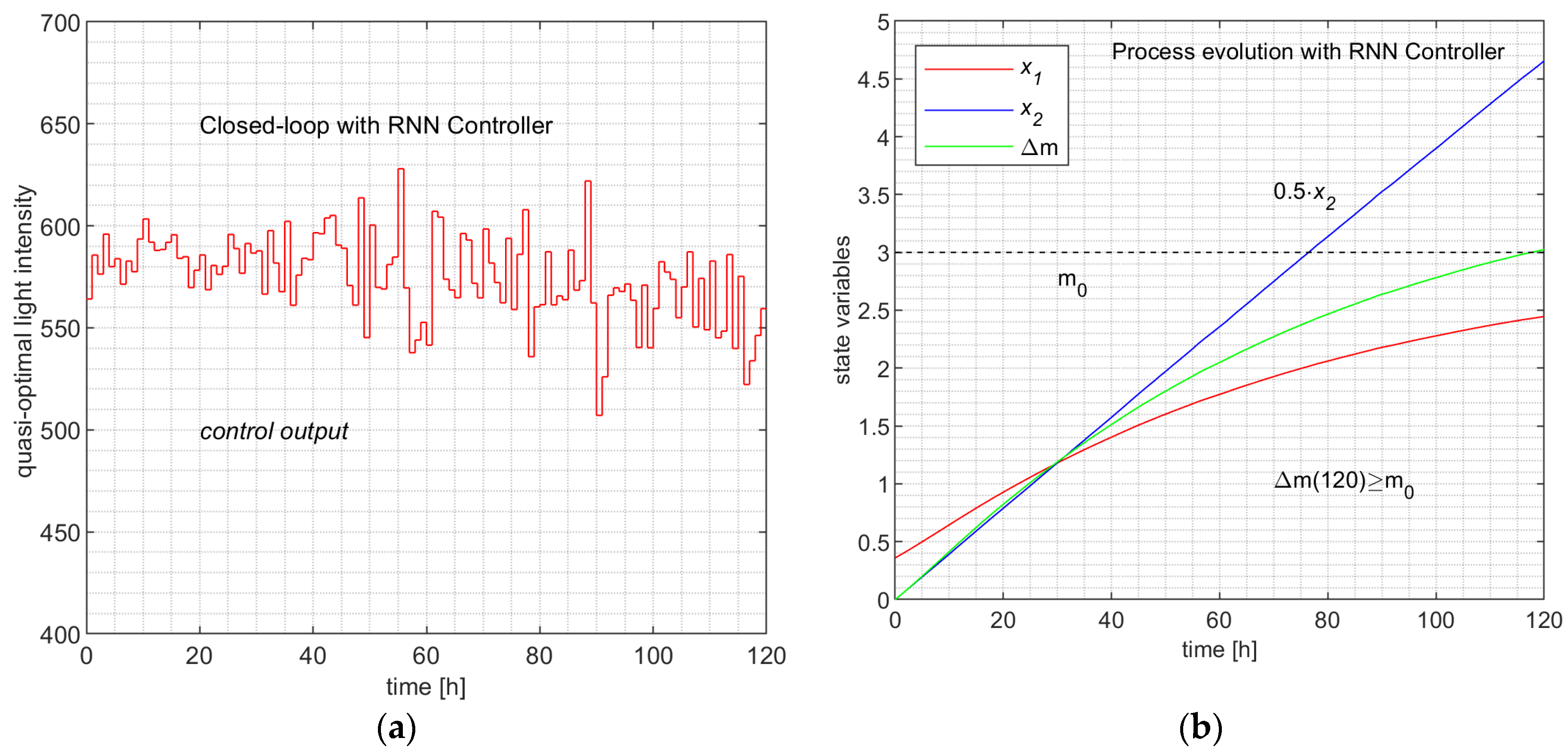
Table 1.
Dataset for step k.
| XT | UT |
| …… | …… |
Table 2.
Pseudocode preparing the data sets for the ML models’ training and testing.
| /*This pseudocode describes the construction of the data sets needed by the ML models at the level of each sampling period*/ Inputs: cell array STATE, matrix UstarRHC; Outputs: matrix SOCSK, table datak, cell arrays DATAKTest, DATAKTrain | |
| 1. | #Load the file containing the data structure STATE and UstarRHC (see Figure 5) |
| 2. | k ← 0 |
| 3. | while k ≤ 0 H-1 |
| 4. | for i=1, ∙∙∙, M |
| 5. | SOCSKi ← [STATEi (k,1:n) UstarRHC(i,k)] |
| 6. | end |
| 7. | #Convert the matrix SOCSK into the table datak. |
| 8. | datakTest lines #1 – 60 of datak |
| 9. | datakTrain lines #61 – 120 of datak |
| 10. | DATAKTest datakTest |
| 11. | DATAKTrain datakTrain |
| 12. | |
| 13. | end |
| 14. | #Save the cell array DATAKTrain and DATAKTest in a file. |
Table 3.
The structure of the ML controller’s algorithm.
| The general algorithm of the ML controller | |
|---|---|
| /*The controller program is called at each sampling period, k */ | |
| 1 | Get the current value of the state vector, X(k); /* Initialize */ |
| 2 | Predict the optimal control value using the regression model /* whatever is the regression model’s type */ |
| 3 | Send the optimal control value towards the process. |
| 4 | Wait for the next sampling period. |
Table 4.
The pseudocode of the linear regressions’ construction.
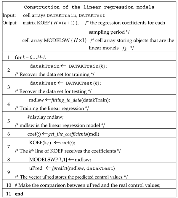
Table 5.
Actions and results of the stepwise linear regression for the 14th sampling period.
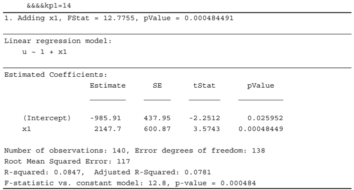
Table 6.
The coefficients of the H linear regressions determined with stepwise strategy.
| k | C0 | C1 | C2 |
|---|---|---|---|
| 0 | 564.18 | 0 | 0 |
| 1 | 585.53 | 0 | 0 |
| 2 | -20.368 | 1441.5 | 0 |
| : | : | : | : |
| 9 | 591.85 | 0 | 0 |
| 10 | 119.74 | 0 | 620.84 |
| 11 | 591.48 | 0 | 0 |
| 12 | 590.95 | 0 | 0 |
| 13 | -985.91 | 2147.7 | 0 |
| 14 | -328.16 | 1205.6 | 0 |
| : | : | : | : |
| 111 | 4055.1 | -1476.6 | 0 |
| 112 | 5482.6 | -2067.6 | 0 |
| 113 | 597.8 | 0 | 0 |
| 114 | 3300.2 | 0 | -308.67 |
| 115 | 587.66 | 0 | 0 |
| 116 | 6446.3 | -2451.2 | 0 |
| 117 | 7144 | -2732.8 | 0 |
| 118 | 4410.7 | 0 | -419.32 |
| 119 | 565.2 | 0 | 0 |
Table 7.
Execution of the closed-loop simulation program (CONTROL_loopLINREG).
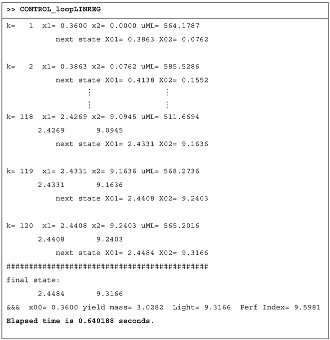
Table 8.
The pseudocode of the regression NNs construction.
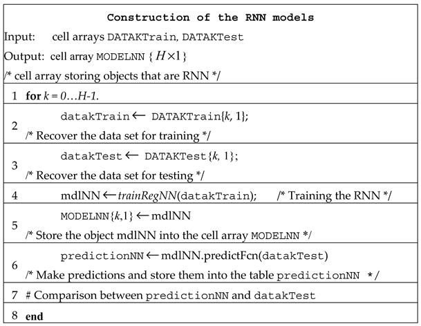
Table 9.
The execution of the RNN training (fragment of the listing)
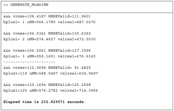
Table 10.
Execution of the closed-loop simulation program (CONTROL_loopNN).
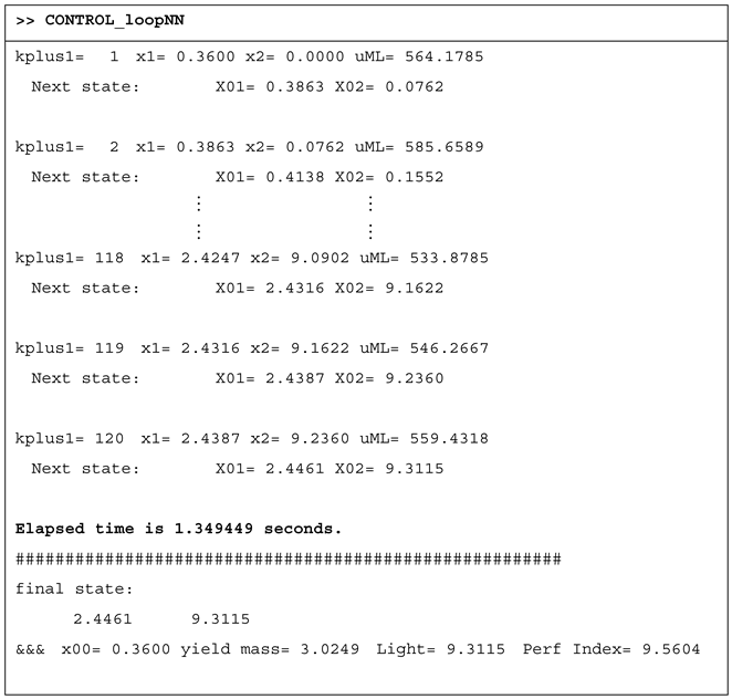
Table 11.
Execution of the closed-loop simulation program (ControlLoop_PSO).
| >>ControlLoop_PSO_RHC |
|---|
| x00= 0.3660 |
| yield mass= 3.0000 |
| Light= 9.2474 |
| Perf Index= 9.2474 |
| Elapsed time is 447.281879 seconds. |
Table 12.
Quantitative comparison among the three controllers.
| PSO Controller | LR Controller | RNN Controller | |
|---|---|---|---|
| x00 | 0.360 | 0.360 | 0.360 |
| yield mass | 3.0000 | 3.0282 | 3.0249 |
| Light | 9.2474 | 9.3166 | 9.3115 |
| Perf Index | 9.2474 | 9.5981 | 9.5604 |
| Control time [s] | 447.28 | 0.64 | 1.35 |
| Training time [s] | - | 5.4 | 232.83 |
| Model size | - | 3 kB | 17 kB |
|
Root Mean Squared Error (RMSE for k=10) |
- | 113.73 | 116.63 |
Disclaimer/Publisher’s Note: The statements, opinions and data contained in all publications are solely those of the individual author(s) and contributor(s) and not of MDPI and/or the editor(s). MDPI and/or the editor(s) disclaim responsibility for any injury to people or property resulting from any ideas, methods, instructions or products referred to in the content. |
© 2024 by the authors. Licensee MDPI, Basel, Switzerland. This article is an open access article distributed under the terms and conditions of the Creative Commons Attribution (CC BY) license (https://creativecommons.org/licenses/by/4.0/).
Copyright: This open access article is published under a Creative Commons CC BY 4.0 license, which permit the free download, distribution, and reuse, provided that the author and preprint are cited in any reuse.


