
Submitted:
02 March 2024
Posted:
04 March 2024
You are already at the latest version
Abstract
Evolutionary algorithms and swarm intelligence algorithms find applicability in reinforcement learning of neural networks due to their independence from gradient-based methods. To achieve successful training of neural networks using these algorithms, careful considerations must be made to select appropriate algorithms due to the availability of various algorithmic variations. In Part1, 2 and 3, the author previously reported experimental evaluations on Evolution Strategy, Genetic Algorithm, and Differential Evolution for reinforcement learning of neural networks, utilizing the Acrobot control task. This article constitutes Part4 of the series of comparative research. In this study, Particle Swarm Optimization is adopted as an instance of major swarm intelligence algorithms. The experimental result shows that PSO performed worse than all of DE, GA and ES. The difference between PSO and DE was statistically significant (p<.01). In addition, PSO exhibited lower capability in exploring solutions in high-dimensional search spaces than DE, GA, and ES did. A larger swarm size compensated for the weakness of PSO in global exploration, thus making itself more beneficial than a larger number of swarm search iterations.
Keywords:
swarm intelligence
; particle swarm optimization
; neural network
; neuroevolution
; reinforcement learning
1. Introduction
Neural networks can be effectively trained using gradient-based methods for supervised learning tasks, where labeled training data are available. However, when it comes to reinforcement learning tasks where labeled training data are not provided, neural networks demand the utilization of gradient-free training algorithms. Evolutionary algorithms [1,2,3,4,5] and swarm intelligence algorithms [6,7,8,9,10] find applicability in the reinforcement learning of neural networks due to their independence from gradient-based methods.
Particle Swarm Optimization [11,12,13], Ant Colony Optimization [14,15], Artificial Bee Colony [16,17], and Cuckoo Search [18,19] are representative swarm intelligence algorithms. To achieve successful training of neural networks using swarm algorithms, careful considerations must be made regarding: i) selecting appropriate algorithms due to the availability of various algorithmic variations, and ii) designing hyperparameters as they significantly impact performance. The author previously reported experimental evaluations on major evolutionary algorithms, Evolution Strategy [20,21], Genetic Algorithm [22,23,24,25], and Differential Evolution [26,27,28], for reinforcement learning of neural networks, utilizing the Acrobot task [29,30,31]. This study applies PSO to the same learning task and compares its performance with those of ES, GA and DE.
2. Acrobot Control Task
As a task that requires reinforcement learning to solve, this study employs Acrobot control task provided at OpenAI Gym. Figure 1 shows a screenshot of the system. This task is the same as that in the previous studies; details on this task were described in Part1 [29]. The same method for scoring fitness of a neural network controller (eq.(1) in Part1) is employed again in this study.
3. Neural Networks
In the previous studies using DE, GA, and ES [29,30,31], the author employed a three-layered feedforward neural network known as a multilayer perceptron (MLP [32,33]) as the controller. The same MLP is utilized again in this study. Figure 2 illustrates the topology of the MLP. The feedforward calculations were described in Part1 [29]. In all of this study and the previous ones, the MLP serves as the policy function: action(t) = F(observation(t)). The input layer consists of six units, each corresponding to the values obtained by an observation. To ensure the input value falls within the range [-1.0, 1.0], the angular velocity of θ1 (θ2) is divided by (). The output layer comprises one unit, and its output value is applied as the torque to the joint.
4. Training of Neural Networks by Particle Swarm Optimization
The three-layered perceptron depicted in Figure 2 includes M+L unit biases and NM+ML connection weights, resulting in a total of M+L+NM+ML parameters. Let D represent the quantity M+L+NM+ML. For this study, the author sets N=6 and L=1, leading to D=8M+1. The training of this perceptron is essentially an optimization of the D-dimensional real vector. Let denote the D-dimensional vector, where each corresponds to one of the D parameters in the perceptron. By applying the value of each element in to its corresponding connection weight or unit bias, the feedforward calculation (described by Equations. (2)–(6) in Part1 [29]) can be processed.
In this study, PSO is applied to optimize the D-dimensional vector . PSO represents one of the swarm intelligence algorithms, which are characterized by being population-based stochastic search algorithms. PSO utilize as a particle position in the D-dimensional search space. The fitness of is evaluated based on eq. (1) described in Part1 [29]. Figure 3 illustrates the PSO process. Steps 1-3 are the same as those in Evolution Strategy, which are described in Part1 [29]. Step 1 initializes vectors , , …, randomly within a predefined range, denoted as , where represents the number of particles (the swarm size). In Step 2, the values in each vector (s=1, 2, ..., ) are fed into the MLP, which subsequently controls the Acrobot system for a single episode consisting of 200 time steps. The fitness of is evaluated based on the outcome of the episode. In Step 3, the iterative training loop concludes upon meeting a preset condition. A straightforward example of such a condition is reaching the limit number of fitness evaluations. In Step 4, the personal best (Pbest) of each particle and the global best (Gbest) in the swarm are updated according to their fitness scores. The Pbest of a particle represents the position vector that has achieved the highest fitness score up to the current iteration for that specific particle. On the other hand, the Gbest represents the position vector with the highest fitness score among all the Pbests in the swarm. Let us denote each Pbest as and the Gbest as , respectively. In Step 5, the velocity of each particle is updated. Let represents the velocity for the s-th particle (s=1, 2, ..., ). The velocity is updated by eq. (1), where denotes the inertia weight, is the Pbest coefficient, and is the Gbest coefficient. Additionally, and are uniformly distributed random numbers within the interval [0,1]. In Step 6, each particle moves in the search space according to its velocity. The position vector is updated by eq. (2).
5. Experiment
In the previous studies using DE, GA, and ES, the number of fitness evaluations included in one experiment trial was set to 5,000 [29,30,31]. The number of new offsprings generated per generation, , was either of (a) 10 and (b) 50. The number of generations was 500 for (a) and 100 for (b) respectively. The total number of fitness evaluations were 10 × 500 = 5,000 for (a) and 50 × 100 = 5,000 for (b). The experiment using PSO in this study employed the same settings to fairly compare PSO with DE, GA and ES. The hyperparameter configurations for PSO are shown in Table 1. The values of w, cp and cg adopted in this study are those suggested by Eberhart and Shi [34]. The domain of particle position vectors, , was kept consistent with the previous experiments [29,30,31], i.e., [-10.0, 10.0]D. The number of hidden units, M, was also consistently set to the four variations: 4, 8, 16, and 32. An MLP with either of 4, 8, 16, or 32 hidden units underwent independent training 11 times. Table 2 presents the best, worst, average, and median fitness scores of the trained MLPs across the 11 trials. Each of the two hyperparameter configurations (a) and (b) in Table 1 was applied.
Comparing the scores in Table 2 between configurations (a) and (b), 12 of the 16 scores (12/16 = 75%) obtained using configuration (b) are larger than their corresponding scores obtained using configuration (a). The Wilcoxon signed rank test confirmed that the difference between scores of configuration (b) and those of (a) was statistically significant (p < .01). This result is consistent with the previous study [29] in which, instead of PSO, ES was adopted as the optimization algorithm. Configuration (a) promotes exploitation in the later stage of search due to the large number of iterations, and configuration (b) promotes exploration in the early stage of search due to the large number of particles. PSO is criticized for its tendency towards premature convergence due to the influence of Gbest, excelling in local exploitation but struggling with global exploration. This weakness, shared with ES, lies in its limited capability for global exploration. Configuration (b) can compensate for this weakness, thus making configuration (b) more beneficial than configuration (a) for both PSO and ES.
Next, upon comparing the fitness scores obtained using configuration (b) among the four variations of M (the number of hidden units), it is observed that the four scores with M=32 are found to be smaller than those with M=4, 8, and 16. No clear superiority is observed among the scores with M=4, 8, and 16. The Wilcoxon rank sum test confirmed that the scores with M=32 are significantly smaller than those with M=4 (p < .05). While no significant differences were observed between the scores with M=32 and those with M=8, 16 (p= .12 and .28 respectively), these p-values indicate that the scores with M=32 were inferior to those with M=8, 16. The scores with M=4 are comparable to those with M=8 (p= .47) and superior to those with M=16 (p= .28). From the perspective of model size and performance, M=4 can be considered the most desirable in this study. Previous studies [29,30,31] employing DE, GA, and ES indicated that M=8, rather than M=4, was the most desirable, with statistically significant differences observed (p < .05 for DE and GA, p < .01 for ES). Based on the results of the past studies and the current study, it is suggested that PSO exhibits lower capability in exploring solutions in high-dimensional search spaces than DE, GA, and ES did. Consequently, M=4, where the dimensionality D is minimum, is deemed preferable. The performance differences between PSO and DE, GA, ES will be further discussed in the subsequent Section 6.
Figure 4 presents learning curves of the best, median, and worst runs among the 11 trials where the configuration is (b). Note that the horizontal axis of these graphs is in a logarithmic scale. The shapes of these graphs are similar to those obtained using DE, GA, and ES [29,30,31]. However, a significant difference is that in the case of PSO, the final fitness scores after the 5000 evaluations are scattered between trials. For all M=4, 8, 16, 32, the differences between the best and the worst trials are large. In previous studies using DE, GA, and ES, these differences were much smaller than those in the case of PSO. In other words, when using DE, GA, and ES, good solutions were stably found without depending on the differences in random initial solutions. However, the results of this experiment indicate that PSO is prone to variability in solution exploration performance depending on the differences in random initial solutions.
Figure 5(a) illustrates the actions by the MLP and the heights py(t) (see eq. (1) in Part1 [29]) in the 200 steps prior to training, while Figure 5(b) displays the corresponding actions and heights after training. Supplementary videos are provided which demonstrate the motions of the chain2,3. In this scenario, the MLP employed 4 hidden units, and the configuration (b) in Table 1 was utilized. In the previous articles [29,30,31] which reported the corresponding results by DE, GA and ES, the actions and the heights are illustrated in Figure 5(a)(b). Comparing the four Figure 5(a) for PSO, DE, GA, and ES, in each case, the MLP before the training continuously output values close to 1.0 (or -1.0) for the entire 200 steps, resulting in the Acrobot chain being unable to move much, and the heights py(t) remaining almost unchanged from its initial value of 0.0. On the other hand, comparing the four Figure 5(b) for PSO, DE, GA, and ES, the shapes of the graphs are similar. The graph for PSO is particularly similar to the graphs for GA and DE: after the heights py(t) exceeded 0.5 around 75 steps, the number of times py(t) fell below 0.5 was small. This indicates that the trained MLP was able to skillfully control the torque to avoid the free end of the Acrobot chain from falling back to a low position after lifting it to a high position. However, even in the case of PSO, it was not possible for the trained MLP to maintain the entire chain in an inverted state and bring the free end of the chain to the highest position at 1.0, which was the same as the results with DE, GA, and ES.
6. Statistical Test to Compare Pso with De, Ga, And Es
The author conducted a Wilcoxon signed rank test to investigate whether there was a statistically significant difference between the fitness scores obtained from the previous experiments using DE, GA or ES and those from the experiment using PSO in this study. The data used for this test included the 32 values reported in Table 2 of Part1 [29] (the data obtained using ES), those in Table 2 of Part2 [30] (the data obtained using GA), those in Table 2 of Part3 [31] (the data obtained using DE), and those in Table 2 of this article (the data obtained using PSO). The test result indicates that the fitness scores by PSO are significantly smaller than those by DE (p < .01). Although the differences between the fitness scores by PSO and those by GA or ES are not statistically significant, the p-values reveals that the scores by PSO are smaller than those by GA (p=.25) and those by ES (p=.07). These test results indicate that, on the MLP training task in this study, PSO performs significantly worse than DE and also performs worse than GA and ES. It is known that particles controlled by PSO are prone to being trapped in local optima, and various improvements have been proposed to address this drawback (e.g. [35]). Future research will be necessary to evaluate the effectiveness of these improvements on this training task.
7. Conclusion
In this study, Particle Swarm Optimization was applied to the reinforcement learning of a neural network controller for the Acrobot task, and the result was compared with that previously reported in Part1/2/3 [29,30,31] where ES/GA/DE was applied to the same task respectively. The findings from this study are summarized as follows:
- (1)
- The statistical tests revealed that PSO performed worse than all of DE, GA and ES. The difference between PSO and DE was statistically significant (p<.01).
- (2)
- The experiment in this study employed two configurations, which are consistent with the previous studies reported in Part1-3: maintaining a fixed number of 5000 fitness evaluations, (a) a greater number of particles, suitable for early-stage global exploration, and (b) a greater number of iterations, suitable for late-stage local exploitation. A comparative analysis of the results revealed that configuration (b) contributed significantly better than configuration (a). Configuration (b) can compensate for the limited capability of PSO in global exploration, thus making itself more beneficial than configuration (a). This result is consistent with the previous study in which ES was adopted [29].
- (3)
- Four different numbers of units in the hidden layer of the multilayer perceptron were compared: 4, 8, 16, and 32. The experimental results revealed that 4 units were found to be the optimal choice from the perspective of the trade-off between performance and model size. This result does not align with previous studies: 8 units were the best in the cases of DE, GA, and ES. PSO exhibited lower capability in exploring solutions in high-dimensional search spaces than DE, GA, and ES did.
The author plans to further apply and evaluate another evolutionary/swarm algorithms to the same task and compare the performance with those by PSO, DE, GA, and ES.
Acknowledgments
The author conducted this study under the Official Researcher Program of Kyoto Sangyo University.
References
- Bäck, T.; Schwefel, H.P. An overview of evolutionary algorithms for parameter optimization. Evolutionary computation 1993, 1, 1–23. [Google Scholar] [CrossRef]
- Fogel, D.B. An introduction to simulated evolutionary optimization. IEEE transactions on neural networks 1994, 5, 3–14. [Google Scholar] [CrossRef] [PubMed]
- Bäck, T. Evolutionary algorithms in theory and practice: evolution strategies, evolutionary programming, genetic algorithms. Oxford university press, 1996.
- Eiben, Á.E.; Hinterding, R.; Michalewicz, Z. Parameter control in evolutionary algorithms. IEEE transactions on evolutionary computation 1999, 3, 124–141. [Google Scholar] [CrossRef]
- Eiben, Á.E.; Smith, J.E. Introduction to evolutionary computing. Springer-Verlag Berlin Heidelberg, 2015.
- Bari, A.; Zhao, R.; Pothineni, J.S.; Saravanan, D. Swarm intelligence algorithms and applications: an experimental survey. Advances in swarm intelligence, ICSI 2023, Lecture notes in computer science, 13968, Springer, 2023.
- Tang, J.; Liu, G.; Pan, Q. A review on representative swarm intelligence algorithms for solving optimization problems: applications and trends. IEEE/CAA journal of automatica sinica 2021, 8, 1627–1643. [Google Scholar] [CrossRef]
- Mavrovouniotis, M.; Li, C.; Yang, S. A survey of swarm intelligence for dynamic optimization: algorithms and applications. Swarm and evolutionary computation 2017, 33, 1–17. [Google Scholar] [CrossRef]
- Payal, M.; Kumar, A.; Díaz, V.G. A fundamental overview of different algorithms and performance optimization for swarm intelligence. Swarm intelligence optimization: algorithms and applications 2020, 1-19.
- Chu, SC.; Huang, HC.; Roddick, J.F.; Pan, JS.. Overview of algorithms for swarm intelligence. Computational collective intelligence, technologies and applications. ICCCI 2011. Lecture notes in computer science, 6922, Springer, 2011.
- Kennedy, J.; Eberhart, R. Particle swarm optimization. Proceedings of ICNN’95 - International conference on neural networks 1995, 4, 1942–1948. [Google Scholar]
- Eberhart, R.; Kennedy, J. A new optimizer using particle swarm theory. MHS’95. Proceedings of the sixth international symposium on micro machine and human science 1995, 39-43.
- Shi, Y.; Eberhart, R. A modified particle swarm optimizer. IEEE international conference on evolutionary computation proceedings 1998, 69–73. [Google Scholar]
- Dorigo, M.; Maniezzo, V.; Colorni, A. Ant system: optimization by a colony of cooperating agents. IEEE transactions on systems, man, and cybernetics, part b (cybernetics), 1996, 26, 29–41. [Google Scholar] [CrossRef]
- Dorigo, M.; Gambardella, L.M. Ant colony system: a cooperative learning approach to the traveling salesman problem. IEEE Transactions on evolutionary computation 1997, 1, 53–66. [Google Scholar] [CrossRef]
- Karaboga, D.; Basturk, B. Artificial bee colony (ABC) optimization algorithm for solving constrained optimization problems. International fuzzy systems association world congress 2007, 789–798. [Google Scholar]
- Karaboga, D.; Basturk, B. A powerful and efficient algorithm for numerical function optimization: artificial bee colony (ABC) algorithm. Journal of global optimization 2007, 39, 459–471. [Google Scholar] [CrossRef]
- Yang, X.S.; Deb, S. Cuckoo search via Lévy flights. IEEE world congress on nature & biologically inspired computing 2009, 210-214.
- Yang, X.S.; Deb, S. Engineering optimisation by cuckoo search. International journal of mathematical modelling and numerical optimisation 2010, 1, 330–343. [Google Scholar] [CrossRef]
- Schwefel, H.P. Evolution strategies: A family of non-linear optimization techniques based on imitating some principles of organic evolution. Annals of operations research 1984, 1, 165–167. [Google Scholar] [CrossRef]
- Beyer, H.G.; Schwefel, H.P. Evolution strategies – a comprehensive introduction. Natural computing 2002, 1, 3–52. [Google Scholar] [CrossRef]
- Goldberg, D.E.; Holland, J.H. Genetic algorithms and machine learning. Machine learning 1988, 3, 95–99. [Google Scholar] [CrossRef]
- Holland, J.H. Genetic algorithms. Scientific American 1992, 267, 66–73. [Google Scholar] [CrossRef]
- Mitchell, M. An introduction to genetic algorithms. MIT press, 1998.
- Sastry, K.; Goldberg, D.; Kendall, G. Genetic algorithms. Search methodologies: introductory tutorials in optimization and decision support techniques 2005, 97-125.
- Storn, R.; Price, K. Differential evolution – a simple and efficient heuristic for global optimization over continuous spaces. Journal of global optimization 1997, 11, 341–359. [Google Scholar] [CrossRef]
- Price, K.; Storn, R.M.; Lampinen, J.A. Differential evolution: a practical approach to global optimization. Springer science & business media, 2006.
- Das, S.; Suganthan, P.N. Differential evolution: a survey of the state-of-the-art. IEEE transactions on evolutionary computation 2010, 15, 4–31. [Google Scholar] [CrossRef]
- Okada, H. Evolutionary reinforcement learning of neural network controller for Acrobot task – Part1: evolution strategy. Preprints.org 2023. [Google Scholar] [CrossRef]
- Okada, H. Evolutionary reinforcement learning of neural network controller for Acrobot task – Part2: genetic algorithm. Preprints.org 2023. [Google Scholar] [CrossRef]
- Okada, H. Evolutionary reinforcement learning of neural network controller for Acrobot task – Part3: differential evolution. Preprints.org 2024. [Google Scholar] [CrossRef]
- Rumelhart, D.E.; Hinton, G.E.; Williams, R.J. Learning internal representations by error propagation. Parallel distributed processing: explorations in the microstructure of cognition 1986, vol.1: foundations. MIT Press, 318-362.
- Collobert, R.; Bengio, S. Links between perceptrons, MLPs and SVMs. Proceedings of the twentyfirst international conference on machine learning (ICML 04), 2004. [CrossRef]
- Eberhart, R.C.; Shi, Y. Comparing inertia weights and constriction factors in particle swarm optimization. Proceedings of the 2000 congress on evolutionary computation (CEC00) 2000, 1, 84–88. [Google Scholar]
- Bonyadi, M.R.; Michalewicz, Z. Analysis of stability, local convergence, and transformation sensitivity of a variant of the particle swarm optimization algorithm. IEEE transactions on evolutionary computation 2015, 20, 370–385. [Google Scholar] [CrossRef]
Figure 1.
Acrobot system1.
Figure 1.
Acrobot system1.
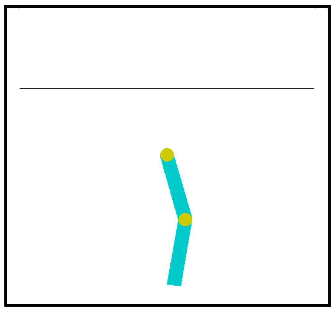
Figure 2.
Topology of the MLP.
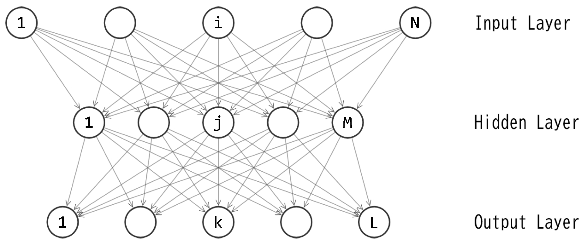
Figure 3.
Process of Particle Swarm Optimization.
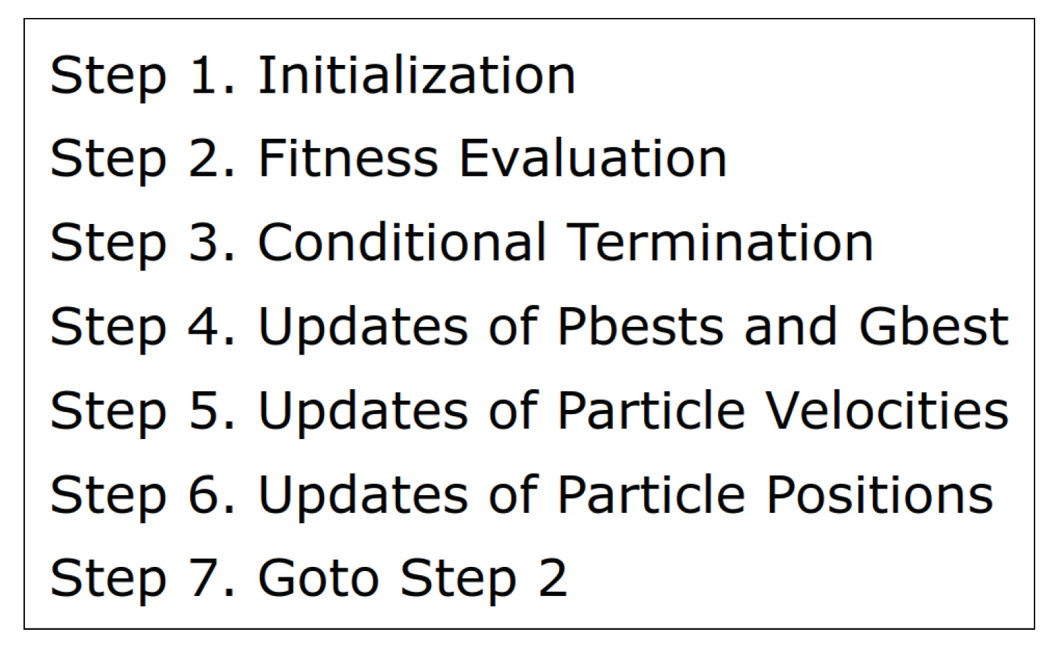
Figure 4.
Learning curves of MLP with M hidden units.
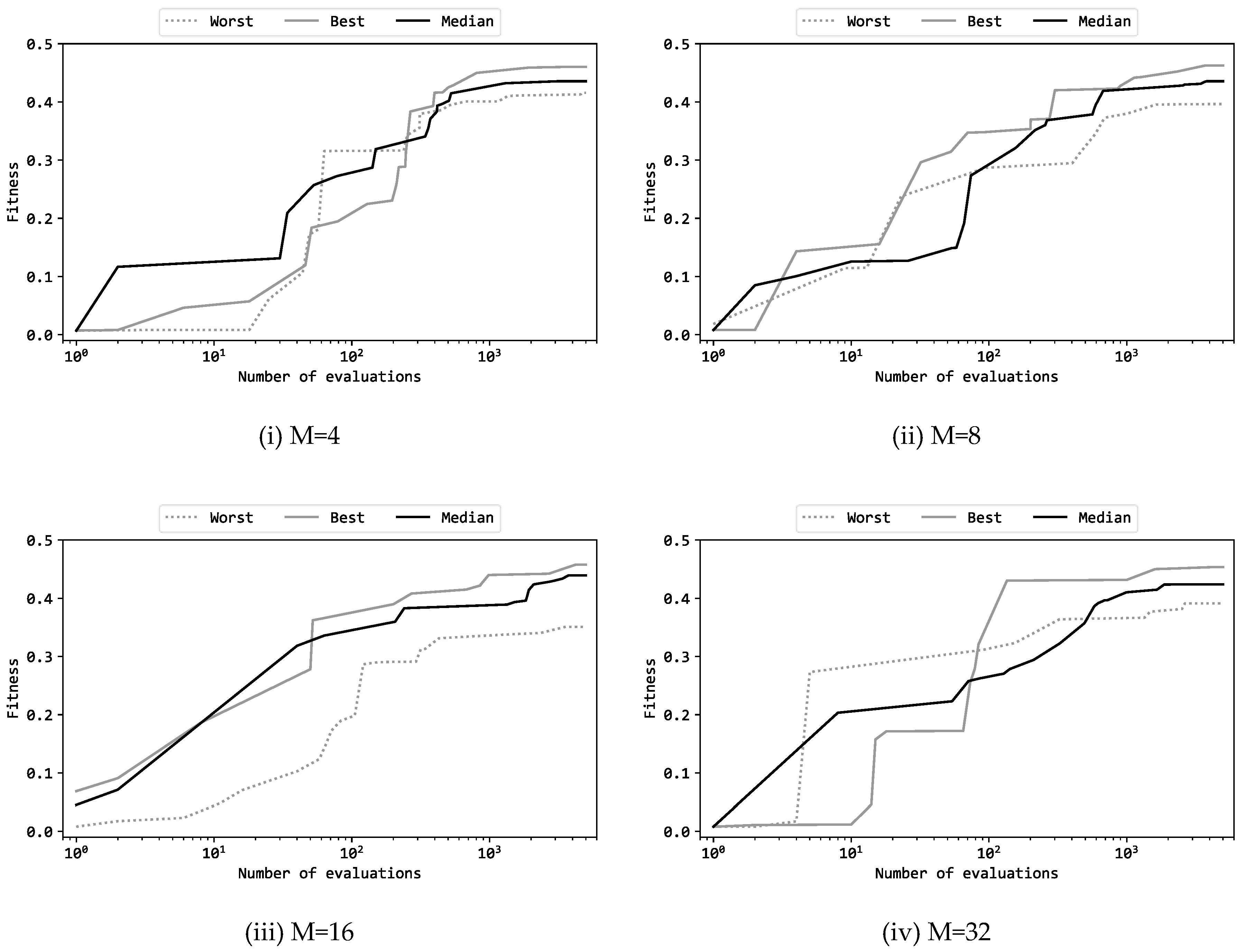
Figure 5.
MLP actions and the height py(t) in an episode.
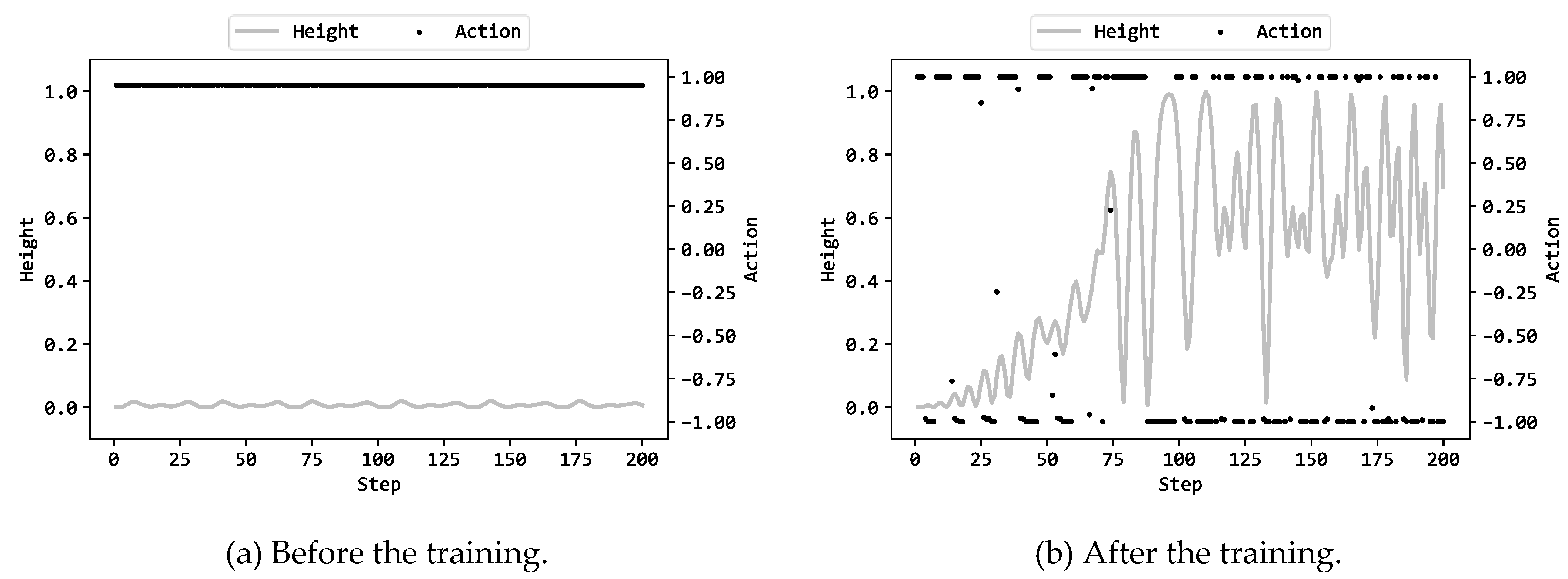

Table 1.
PSO Hyperparameters.
| Hyperparameters | (a) | (b) |
|---|---|---|
| Number of particles () | 10 | 50 |
| Iterations | 500 | 100 |
| Fitness evaluations | 10500=5,000 | 50100=5,000 |
| Inertia weights (w) | 0.729 | 0.729 |
| Pbest coefficient (cp) | 1.49445 | 1.49445 |
| Gbest coefficient (cg) | 1.49445 | 1.49445 |
Table 2.
Fitness Scores among 11 Runs.
| M | Best | Worst | Average | Median | |
|---|---|---|---|---|---|
| (a) | 4 | 0.469 | 0.336 | 0.408 | 0.417 |
| 8 | 0.450 | 0.269 | 0.401 | 0.435 | |
| 16 | 0.467 | 0.333 | 0.424 | 0.439 | |
| 32 | 0.465 | 0.314 | 0.418 | 0.425 | |
| (b) | 4 | 0.460 | 0.416 | 0.440 | 0.436 |
| 8 | 0.463 | 0.396 | 0.437 | 0.436 | |
| 16 | 0.458 | 0.351 | 0.429 | 0.439 | |
| 32 | 0.453 | 0.391 | 0.425 | 0.424 |
Disclaimer/Publisher’s Note: The statements, opinions and data contained in all publications are solely those of the individual author(s) and contributor(s) and not of MDPI and/or the editor(s). MDPI and/or the editor(s) disclaim responsibility for any injury to people or property resulting from any ideas, methods, instructions or products referred to in the content. |
© 2024 by the authors. Licensee MDPI, Basel, Switzerland. This article is an open access article distributed under the terms and conditions of the Creative Commons Attribution (CC BY) license (http://creativecommons.org/licenses/by/4.0/).
Copyright: This open access article is published under a Creative Commons CC BY 4.0 license, which permit the free download, distribution, and reuse, provided that the author and preprint are cited in any reuse.


