Submitted:
18 April 2024
Posted:
19 April 2024
You are already at the latest version
Abstract
Being able to express broad families of equivariant or invariant attributed graph functions is a popular measuring stick of whether graph neural networks should be employed in practical applications. However, it is equally important to learn deep local minima of losses (i.e., with much smaller loss values than other minima), even when architectures cannot express global minima. In this work we introduce the architectural property of attracting GNN optimization trajectories to local minima as a means of achieving smaller losses. We take first steps in satisfying this property for losses defined over attributed undirected unweighted graphs with a novel architecture, called Universal Local Attractor (ULA). The latter refines each dimension of end-to-end trained node feature embeddings based on graph structure to track the optimization trajectories of losses satisfying some mild conditions. The refined dimensions are then linearly pooled to create predictions. We experiment on 10 tasks, from node classification to clique detection, on which ULA is comparable with or significantly outperforms popular alternatives of similar or greater theoretical expressive power.
Keywords:
Graph Neural Networks
; Universal Approximation
; Local Attractors
; Diffusion
; Attributed Graphs
1. Introduction
Graph Neural Networks (GNNs) are a machine learning paradigm that processes graph structured data by exchanging representations between linked nodes. Despite this paradigm’s empirical success in tasks like node or graph classification, there are emerging concerns on its general applicability. Research has so far focused on the expressive power of GNNs, namely their ability to tightly approximate attributed graph functions (AGFs). These take as input graphs whose nodes contain attribute vectors, such as features, embeddings, or positional encodings and create node or graph predictions (Section 2.3). Practically useful architectures, i.e., with a computationally tractable number of parameters that process finite graphs, have been shown to express certain families of AGFs, such as those that model WL-k tests (Section 2.3). In set theory terminology (Appendix A), architectures are dense in the corresponding families.
Although satisfying WL-k or other tests is often taken as a golden standard of expressive power, it does not ensure that losses corresponding to training objectives are straightforward to minimize [1], or that expressive power is enough to replicate arbitrary objectives. Therefore, applied GNNs should also easily find deep loss minima, in addition to any expressive power guarantees. In this work, the concept of deep minima refers to empirically achieving small loss values compared to other local minima. Although these values may not necessarily be close to the globally best minimum (e.g., zero), they can still be considered better training outcomes compared to alternatives. We refer to minima that are not deep as shallow. These characterizations are informal, and demonstrated in Figure 1 for a real-valued loss function. Non-global minima in the figure are “bad local valleys” [2,3] in that they may trap optimization to suboptimal solutions. However the premise of this work is that deep minima are acceptable given that they exhibit small enough loss values.
In detail, we argue that the main challenge in deeply minimizing GNNs lies with the high-dimensional nature of loss landscapes defined over graphs, which exhibit many shallow valleys.1 That is, there are many local minima with large loss values, corresponding to “bad” predictive ability, and optimization runs the risk of arriving near those and get trapped there. To understand this claim, Figure 2 presents the landscape of a loss defined on one triangle graph (i.e., three nodes linked pairwise). The third node makes optimization harder by creating many local minima of various depths when it obtains suboptimal values, for example imposed by GNN architectures. We seek strategies that let deep minima attract optimization trajectories (as observed in the space of node predictions) while confining local minima attraction to small areas, for example that initialization is unlikely to start from, or that the momentum terms of machine learning optimizers can escape from [4]. Theoretical justification of this hypothesis is left for future work, as here we probe whether architectures exhibiting local attraction properties can exist in the first place.
Universally upholding local attraction is similar to universal approximation barring two key differences: First, attraction is weaker in that it attempts to find local loss minima instead of tightly approximating functions (it approximates zero loss gradients instead of zero loss). Second, the proposition is broader than many universal approximation results for practical architectures in that it is “universal” on more objectives (it is not restricted to tests like WL-k, even when the expressive power exhibits such restrictions). Here, we achieve local attraction with a novel GNN architecture, called Universal Local Minimizer (ULA). The mild conditions under which this architecture is universal can be found in Section 6.3. The process we follow to build it consists of three steps, which start from simple and progressively move to more complex settings:
- Step 1.
- We analyse positive definite graph filters, which are graph signal processing constructs that diffuse node representations, like embeddings of node features, through links. Graph filters are already responsible for the homophilous propagation of predictions in predict-then-propagate GNNs (Section 2.2) and we examine their ability to track optimization trajectories of their posterior outputs when appropriate modifications are made to inputs. In this case, both inputs and outputs are one-dimensional.
- Step 2.
- By injecting the prior modification process mentioned above in graph filtering pipelines, we end up creating a GNN architecture that can minimally edit input node representations to locally minimize loss functions given some mild conditions.
- Step 3.
- We generalize our analysis to multidimensional node representations/features by folding the latter to one-dimensional counterparts while keeping track of which elements correspond to which dimension indexes, and transform inputs and outputs through linear relations to account for a different dimensions between them.
In experiments across 11 tasks, we explore the ability of ULA to learn deep minima by comparing it to several well-known GNNs of similar predictive power on example synthetic and real-world predictive tasks. In these, it remains consistently similar or better than the best-performing alternatives in terms of predictive performance, and always the best in terms of minimizing losses. Our contribution is threefold:
- a.
- We introduce the concept of local attraction as a means of producing architectures whose training can reach deep local minima of many loss functions.
- b.
- We develop ULA as a first example of an architecture that satisfies local attraction given the mild conditions summarized in Section 6.3.
- c.
- We experimentally corroborate the ability of ULA to find deep minima on training losses, as indicated by improvements compared to performant GNNs in new tasks.
This work is structured as follows. After this introductory section, Section 2 presents background on graph filters, graph neural networks, and related universal approximation terminology and results. Section 3 formalizes the local attraction property, and presents extensive theoretical analysis that incrementally constructs a first version of the ULA architecture that parses one-dimensional node features; we call this ULA1D. Section 4 generalizes ULA1D to multi-dimensional node features and outputs to obtain ULA, and describes the latter’s theoretical properties and implementation needs. Section 5 presents experimental validation of our architecture’s—and by extend the local attraction property’s—practical usefulness by showing that it finds similar or much deeper local minima than competitive alternatives across a collection of six synthetic and real-world settings. Section 6 discusses how ULA should be applied in practice, as well as threats to this work’s validity. Finally, Section 7 summarizes our findings and presents prospective research directions.
2. Background
2.1. Graph Filters
Graph signal processing [5] extends traditional signal processing to graph-structured data by defining graph signals that assign real values to nodes (nodes and their integer identifiers are used interchangeably). They make use node adjacency matrices M whose elements hold either edge weights (1 for unweighted graphs) or zeros if the corresponding edges do not exist. Adjacency matrices are normalized as:
where D is the diagonal matrix of node degrees. Iterative matrix-vector multiplications express the propagation hops away of h. Throughout this work we adopt symmetrically normalized adjacency matrices of the second kind, as they are also employed by Graph Convolutional Networks (GCNs of Section 2.2). A weighted aggregation of hops defines graph filters and their posteriors r per:
for weights indicating the importance placed on propagating graph signals n hops away. In this work, we focus on graph filters that are positive definite matrices, i.e., whose eigenvalues are all positive. We also assume a normalization for all filters, for which the maximum eigenvalue of the filter becomes:
for the range of eigenvalues for symmetrically normalized adjacency matrices . Two well-known filters of this kind are personalized PageRank [6] and Heat Kernels [7]. These respectively arise from power degradation of hop weights and the exponential kernel for parameters and .
2.2. Graph Neural Networks
Graph neural networks apply diffusion principles to multidimensional node features, for example by defining layers that propagate nodes features to neighbors one hop away, aggregating (e.g., averaging) them there, and transforming the result through linear neural layers with non-polynomial activation. To avoid oversmoothing that limits architectures to a couple of layers that do not to account for nodes many hops away, recursive schemes have been proposed to partially maintain early representations. Of these, our approach reuses the computational scheme of the predict-then-propagate architecture, known as APPNP [8], which decouples the neural and graph diffusion components by first enlisting multilayer perceptrons to end-to-end train representations of node features H by stacking linear layers ℓ endowed with activation [9], and then applying the personalized PageRank filter on each representation dimension to arrive at final node predictions:
A popular family of architectures that are often encountered as a concept throughout this work are Message-Passing GNNs (MPNNs) [10]. These aggregate representations from node neighborhoods, combine them with each node’s own representation, and propagate them anew. Layers of this family can be written as:
where the activation is the relu function in intermediate layers and, for classification tasks, becomes a softmax at the top representation layer. The mechanism is typically a row-wise concatenation followed by a linear layer transformation. It may also include element-by-element multiplication to be able to express the full class of WL-1 test, as GNNML1 does [11]. The aggregation step often accounts for some notion of neighborhood around each node and can be as simple as an average across neighbors per after adding self-loops to the graph [12] (adding self-loops is a common practice that is also employed by APPNP), or involve edge-wise attention based on the linked nodes [13]. For completeness, we present the mathematical formula of the Graph Convolutional Network (GCN) architecture’s layers:
where and correspond to trainable weight matrices and broadcasted biases.
2.3. Universal Approximation of AGFs
Typically, GNNs are required to be equivariant or invariant under node permutations. These concepts correspond to outputs following the node permutations or being independent of them respectively. An AGF satisfies these properties if, for all attributed graphs with adjacency matrices M and node features H:
where is a matrix that permutes node order. We treat permutation as an operator. In this work we tackle only equivariance, given that reduction mechanisms across nodes (e.g., an average of all feature values across nodes) turn equivariance into invariance. These properties are not inherently covered by the universal approximation theorems of traditional neural networks, which GNNs aim to generalize. It is, then, of interest to understand the expressive power of architectures given that they satisfy one of the properties. This way, one may get a sense of what to expect from their predictive ability.
Theoretical research has procured various universal approximation theorems for certain architectures that show either a general ability to approximate any AGF or the ability to differentiate graphs up to the Weisfeiler-Lehman isomorphism test of order k (WL-k), which is a weaker version of graph isomorphism. For example, WL-2 architectures can learn to at most recognize triangles but can not necessarily differentiate between more complex structures, as shown in Figure 3. The folkore WL-k (FWL-k) test [14] has also been used as a non-overlapping alternative [15] (there is no clear distinction between the strengths of the two tests). Universal approximation is stronger than both in that it can perfectly detect isomorphism.
Simple architectures, like GNNML1 [11], GCN [12], and APPNP [8], are at most as powerful as the WL-1 test in distinguishing between graphs of different structures, but remain popular for parsing large graphs thanks to their tractable implementations that take advantage of adjacency matrix sparsity to compute forward passes in times where is the number of graph edges and L the number of layers (usually 2,5,10, or 64 depending on the architecture and how well it tackles the oversmoothing problem) are known to be at most as powerful as WL-1. On the other hand, architectures like 1-2-3GNN [16] and PPGN [15] satisfy the WL-3 test but come at the cost of high computational demands (e.g., millions of hidden dimensions) by considering all tuples or triples node pairs, in the last case exhibiting computational complexity where is the number of graph nodes. For a summary on the expressive power of several architectures, refer to the work of Balcilar et al. [11], who also introduce the and GNNML3 architecture to overcome these limits with appropriate injection of spectral node features.
In addition to WL-k or other types of limited expressiveness, some works tackle universal approximation over all AGFs. Historically, deep set learning [17] introduced universal approximation results for equivariant and invariant functions over sets that were quickly generalized to graph structures. However, so powerful architectures also suffer from computational intractability, like unbounded tensor order for internal representations [18], and the tensor order of internal representations needing to be at least half the number of input feature dimensions rounded down [19]. Increasing tensor order dimensions is so computationally intensive that respective works experiment with graphs of few nodes.
An alternate research direction is to create MPNNs that, even though limited to WL-1 expressive power by themselves [16,20], can be strengthened with additional components. To this end, the generic message passing scheme has been shown to be universal over Turing computable functions [1], although this does not cover the case of non-computable functions or density over certain sets of non-computable functions. More recent breakthroughs have shown that the expressive power is not necessarily a property of architectures alone, because enriching the node feature space with positional encodings [21,22,22], like random node representations, can make MPNNs more powerful [23]. A result that we use in later experiments is that MPNNs enriched with non-trainable node representations can express any non-attributed graph functions while retaining equivariance in probability [24].
For a comprehensive framework for working with node encodings, see the work of Keriven et al. [22]. In the latter, the authors criticize random node representations as non-perfectly equivariant, but in this work we adopt that methodology’s motivating viewpoint that, in practice, equivariance in probability by creating random values with the same process for each node is nearly as good as hard-coded equivariance. At the very least, architectures endowed with random node representations can serve as comparisons between ULA and strengthened expressive power.
2.4. Symbols
Here, we summarize symbols that we will be using throughout this work. In general, we use calligraphic letters to denote sets and parameterized functions, capital letters to denote matrices, and lower case symbols to denote vectors or numeric values:

Table 1.
| Symbol | Interpretation |
| The set of all AGFs. | |
| A GNN architecture function with parameters . | |
| An attributed graph with adjacency M and features . | |
| The node feature matrix predicted by on attributed graph . | |
| M | A graph adjacency matrix. |
| A finite or infinite set of attributed graphs. | |
| Gradients of a loss computed at | |
| A normalized version of a graph adjacency matrix. | |
| A graph filter of a normalized graph adjacency matrix. It is also a matrix. | |
| X | A node feature matrix. |
| Y | A node prediction matrix of a GNN. |
| R | A node output matrix of ULA1D. |
| H | A node representation matrix, often procured as a transformation of node features. |
| A loss function defined over AGFs A. | |
| A loss function defined over attributed graphs for node prediction matrix Y. | |
| Node representation matrix at layer ℓ of some architecture. Nodes are rows. | |
| Learnable dense transformation weights at layer ℓ of a neural architecture. | |
| Learnable biases at layer ℓ of a neural architecture. | |
| Activation function at layer ℓ of a neural architecture. | |
| The number of columns of matrix . | |
| The integer ceiling of real number x. | |
| The number of set elements. | |
| The set of a graph’s nodes. | |
| The set of a graph’s edges. | |
| A domain in which some optimization takes place. | |
| Parameters leading to local optimum. | |
| A connected neighborhood of . | |
| A graph signal prior from which optimization starts. | |
| A locally optimal posterior graph signal of some loss. | |
| The L2 norm. | |
| The maximum element. | |
| Horizontal matrix concatenation. | |
| Vertical matrix concatenation. | |
| Multiplayer perceptron with trainable parameters θ |
3. One-Dimensional Local Attraction
In Section 3.1 we start by stating the generic form of the local attraction property. We then aim to satisfy that property with GNN architectures that employ positive definite graph filters as methods to diffuse information through edges. To this end, we conduct one-dimensional analysis with graph signals that are column vectors of dimension . These pass though positive definite graph filters to create posteriors . In Section 3.2 we further constrain ourselves to optimization in one graph to create first local attraction properties for posteriors r. A first generalization of results that processes graphs with an upper bounded number of nodes is created in Section 3.3. These results easily generalize to multiple input and output dimensions in the next section.
The universal attractor that parses one-dimensional node representations H of any graph alongside other graph signals required to minimize a loss is called ULA1D. An overview of its feedforward pipeline is described in Figure 5. Broadly speaking, our goal is to learn new priors given all starting information—including original posteriors—that lead us to locally optimal posteriors . This architecture can be trained end-to-end already to let R locally minimize losses. As an intermediate component it uses a Multilayer Perceptron (MLP) to generate updated node representations to be diffused by graph filters. We generalize the architecture to multidimensional graph features with the methodology of Section 4, where multidimensional information is unwrapped to vector form; jump forward to that section’s introduction to get an overview of the final ULA and where ULA1D fits in its forward pipeline.
3.1. Problem Statement
Proposition 1 uses set theory terminology (Appendix A) to express our local attraction property, where refers to the L2 norm. Our hypothesis is that this property is requisite for deeply optimizable GNNs. Intuitively, we seek architectures that, for any local minimum, admit a transformation of parameters that turns a connected neighborhood around the minimum into a loss plateau, i.e., an area with approximately near-zero gradient. We define loss plateaus with respect to gradients of architecture outputs instead of parameter gradients , in order to avoid premature convergence that would “stall” due to architectural computations and not due to actual minimization of the loss. For example, we do not accept architectures that produce constant outputs when those constants are not local loss minima.
Proposition 1
(Locally attractive GNNs). Find architecture with parameters in a connected compact set such that, for any parameters minimizing a differentiable loss and any , there exists a parameter endomorphism S achieving for any parameters in some connected neighborhood of the minimum.
If there exist multiple endomorphisms (i.e., transformations of parameters), one can select those that create plateaus more difficult to escape from for deep minima, but are easier to escape from for shallow local minima. For example, this can be achieved by controlling some the attraction radii of Section 3.2. During this work’s experimental validation, we select radii based on domain knowledge; our analysis reveals that the radii can be controlled by the diffusion rates of graph filters we employ, and thus we look at personalized PageRank filter with a usually well-performing default diffusion parameter. Future research can make a more advanced search for appropriate filters that would create different radii.
Lastly, we tackle training objectives that can be expressed as a collection of sub-losses defined over a collection of attributed graphs with node prior representations H and predicted node output representations R that we aim to discover. We can pool all losses to one quantity for a GNN architecture :
This setting can learn to approximate any equivariant AGFs (any reduction mechanism to node predictions can also learn invariant AGFs), albeit not densely (i.e., not necessarily with arbitrarily small error, for example because there the architecture is not expressive enough). The above setting also lets our analysis create functional approximations to non-functions, for example that may include two conflicting loss terms for the same attributed graph. An implicit assumption of our analysis is that there exist architectural parameters that can replicate at least one local minimum.
3.2. Local Attractors for One-Dimensional Bode Features in One Graph
To remain close to the original outputs of graph filters while also controlling for desired objectives, we adopt practice of adjusting their inputs [25]. If we choose to do so, different outputs are at most as dissimilar as different inputs, given that by definition where is the filter’s maximal eigenvalue when its parameters are normalized. As a first step, we exploit the structural robustness imposed by positive eigenvalues to create a local attraction area for some graph algorithm.
Consider starting priors and a twice differentiable loss on some compact domain that has at least one local minimum (reminders: is the number of nodes, and both priors and posteriors in our current setting are vectors that hold a numeric value for each node). Our goal is to find one such minimum while editing the priors. To this end, we argue that positive definite graph filters are so stable that they require only a rough approximation of the loss’s gradients in the space of priors to asymptotically converge to local optima for posteriors. This observation is codified in Theorem 1. We improve this result in Lemma 2, which sets up prior editing as the convergent point of a procedure that leads to posterior objective optimization without moving too far away from starting priors .
Lemma 1.
For a positive definite graph filter and differentiable loss over graph signal domain , update graph signals over time per:
where are the smallest positive and largest eigenvalues of respectively. This leads to if posteriors remain closed in the domain, i.e., if .
Proof sketch.
Essentially roughly approximates the loss’s gradients. Small non-exact approximation is absorbed by the positive definite filter’s stability. A full mathematical proof is provided in Appendix B.
Lemma 2.
Let a differentiable graph signal generation function2 on compact connected domain Θ admit some parameters such that . If, for any parameters , the Jacobian has linearly independent rows (each row corresponds to a node) and satisfies:
then there exist parameters such that .
Proof schetch.
Empirically, is a matrix that represents differences between the unit matrix. The Jacobian of is multiplied with the right pseudo-inverse of the difference, which will be close to the unit matrix for enough parameters. Otherwise, differences are constrained to matter only for nodes with high score gradient values (non-zero Jacobian elements). Thus, as long as the objective’s gradient retains a clear—though maybe changing—direction to move towards to, that direction can be captured by a prior generation model of few parameters that may (or should) fail at following other kinds of trajectories. If such a model exists, there exists a parameter trajectory it can follow to arrive at locally optimal prior edits. A full mathematical proof is provided in the supplementary material. □
We are now equipped with the necessary theoretical tools to show that neural networks are valid prior editing mechanisms as long as starting priors are close enough to ideal ones and some minimum architectural requirements are met. This constitutes a preliminary local attraction result that applies only to a graph signal processing pipeline and is codified in Theorem 1. A closed expression of the theorem’s suggested architecture follows:
where | is horizontal concatenation, the near-ideal priors are , and represents the trainable multilayer perceptron that computes updated priors and parameters comprise all of its layer weights and biases. represents any additional node information that determines the loss function’s value.
Implementations should follow the dataflow of Figure 4 presented at the beginning of this section. To show the existence of a neural network architecture, we use a specific universal approximation theorem that works well with our theoretical assumptions. However, other linear layers can replace the introduced one; at worst, and without loss of validity, these would be further approximations. The combination of an MLP component with propagation via graph filters sets up our architecture as a variation of the predict-then-propagate scheme after selecting appropriate .
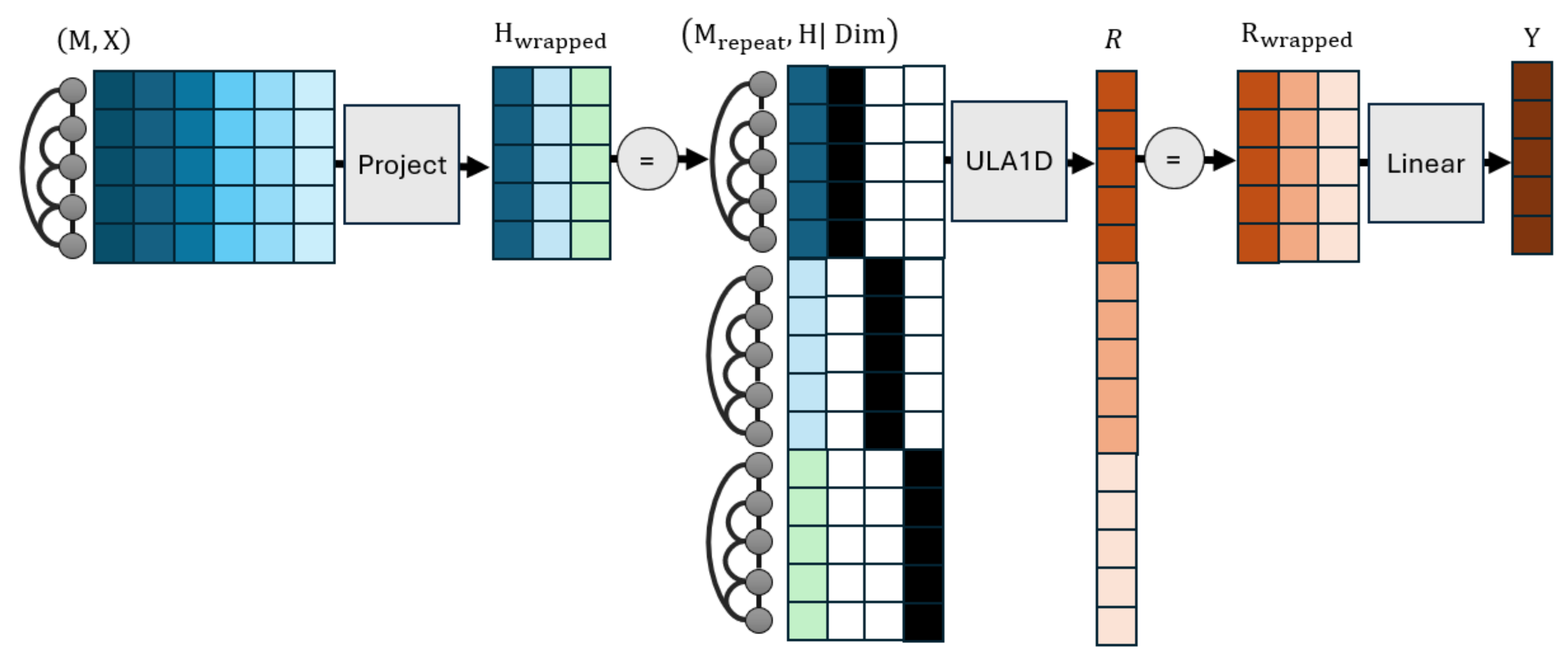
Figure 4.
The one-dimensional universal local attractor (ULA1D) architecture; it obtains the outcome of diffusing the blue prior vector H through adjacency matrix M with a graph filter , and then refines the posteriors. The refinement consists of concatenating the prior, the node information contributing to the loss function (black and white ), and the original posteriors to provide them as inputs to an MLP that learns new priors . These in turn pass through the same graph filter to create new locally optimal posteriors R.
Theorem 1.
Take the setting of Lemma 2, where the loss’s Hessian matrix linearly approximates the gradients within the domain with error at most . Let us construct a node feature matrix whose columns are graph signals (its rows correspond to nodes v). If , , and all graph signals other than r involved in the calculation of are columns of , and it holds that:
for any , then for any there exists with relu activation, for which
Proof sketch.
Thanks to the universal approximation theorem (we use the form presented by [26] to work with non-compact domains and obtain sufficient layer widths), neural networks can produce tight enough approximations of the desired trajectory gradients. At worst, there will be two layers to form a two-layer perceptron. We also use a second set of neural layers on top of the first to compute their integration outcome. A full mathematical proof is provided in Appendix B. □
Theorem 2 shows that any twice differentiable loss can be optimized from points of a local area (i.e., this is a universal local attraction property), given that a sufficiently large L1 posterior regularization has been added to it. Therefore the architecture of Theorem 1 is a local attractor of some unobserved base architecture, an unobserved feature transformation, and an unobserved parameter subdomain that nonetheless creates a known attraction radius in the space of posteriors. Locally optimal posteriors cannot attract all optimization trajectories; the radius of the hypersphere domain from which ideal posteriors can always attract others is at worst .3
If attraction hyperspheres are overlapping between local minima, it is uncertain which is selected. This is why we want to impose local attractiveness in the first place; to minimize overlaps between deep and shallow minima so that optimization can permanently escape from the pull of the latter. Therefore, radii need to be large enough to enclose original posteriors within at least one hypersphere of nearby ideal ones, but not large enough to attract posteriors to shallow optima. For points farther away than the attraction radii from all local minima, it is unclear if any minimum would be found at all by a learning process.
A similar analysis to ours [27] points out that spectral graph theory research should move beyond low-pass filters and graphs with small eigenvalues; in this case, our worst attraction radius provides a rough intuition of which scenarios are easier to address. For example, we can explain why directly optimizing posteriors can lead to shallow optima [27]; direct optimization is equivalent to using the filter , which exhibits large optimization horizon radius , and is therefore likely to enclose many local minima as candidates towards which to adjust posteriors, including shallow ones. Conversely, filters that acknowledge the graph structure play the role of a minimum curation mechanism, which is a popular but previously unproven hypothesis [28,29] that we verify here.
Theorem 2.
There exists sufficiently large parameter for which
satisfies the properties needed by Theorem 1 within the following domain:
where is the ideal posteriors optimizing the regularized loss. If the second term of the max is selected, it suffices to have no regularization .
Proof sketch.
The area from which posteriors can be attracted to local optima is wider the closer to linear posterior objectives are. Furthermore, loss derivatives should also be large enough that, when their norm is multiplied with , they still push optimization trajectories towards minima from faraway points of the domain. Large enough L1 regularization translates to derivative magnitude at each dimension. That is, it introduces a constant push of posteriors towards zero that keeps gradients sufficiently large. A full mathematical proof is provided in Appendix B. □
In the next subsection, we select losses with Lipschitz gradients. This means that Theorem 2 can create constrained attraction radii for given a graph filter with small enough eigenvalue ratio, as long as , which means that the loss should not be exactly the square distance from the starting posteriors. Although we select this losses that satisfy the Lipschitz gradient property throughout the rest of analysis, we keep the more general version of the theorem to support future research directions, if needed.
3.3. Attraction across Multiple Graphs
In Lemma 3 and Theorem 3, we now show that ULA1D (i.e., the architecture of Equation 3) adheres to a universal minimization property over respectively finite and infinite collections of undirected unweighted attributed graphs with a bounded number of nodes. Both results can be applied for variation of the MLP component that use different universal approximation theorems, given that activation functions are still Lipshitz. The second theorem stipulates some additional conditions that let us generalize the architecture’s minimization to infinite sets of attributed graphs with one-dimensional node representations. We consider the conditions mild in that they are easy to satisfy. For example, node features may be (batch-)normalized to make them bounded.
Both theorems require a finite number of nodes of processed graphs to properly work with. This may be larger than the number of nodes in training graphs if similar substructures are encountered, but the theorems do not reveal an upper bound, and thus the latter should be empirically evaluated in practical applications. At the same time, during the proof of Theorem 3 we employ a graph with a non-polynomial number of nodes that represents an equivalently hard problem. Theoretically, this means that our architecture could require a non-polynomial (though bounded) number of training data samples to learn under the required local attraction concerns. This only affects generalization power given the number of samples, i.e., whether low training and validation losses translate to low test losses, and is easy to check for in practice. Importantly, the space ULA1D implementations (and, by extension, the ULA implementation when we extend results to multidimensional node representations) is not only dense on local attractors but can actually reach them given enough training samples.
A final caveat of Theorem 3 is that, for MLP activations that are not differentiable everywhere, the property of remaining in the local attraction area can theoretically be guaranteed only in probability. In particular there may exist points with “infinite” derivatives that may propel losses outside that area. In practice, though, activation functions are computed on finite machines where twice differentiable relaxations can be considered in areas smaller than the numerical tolerance without affecting computational results. In this case, the dense subset of the neighborhood coincides with the full neighborhood. The theorem’s version we present is geared towards future investigations of how limits in numerical tolerance could affect the local attraction property in practice.
Lemma 3.
Let a finite set of attributed graphs with undirected unweighted adjacency matrices M with up to a finite number of nodes v and one-dimensional node representations H be denoted as . Let loss be twice diffentiable with respect to r and take any . Then any selected that lets Equation 3 be local loss minimum on all attributed graphs of is contained in a connected neighborhood of for which:
Proof sketch.
We generate a larger graph that comprises all subgraph structures and vertically concatenates corresponding node features. Thus, by reframing the small derivative outcome as an objective on this new attributed graph, Theorem 2 lets us minimize it to arbitrarily small derivative. A full mathematical proof is provided in Appendix B. □
Theorem 3.
Consider infinite sets , bounded node feature values, Lipshitz loss gradients with respect to both h and r, and that has activation functions that are almost everywhere Lipshitz with Lipshitz derivatives (e.g., relu). Then, Lemma 3 holds for a dense subset of the neighborhood.
Proof sketch.
Given that both the architecture and loss gradients are Lipshitz, similar pairs of node features will create similar gradients for the same adjacency matrices. We thus create a discretization of the domain of node features with small numerical tolerance. In this discretization, there is a finite number of possible adjacency matrices given the bounded number of graph nodes, and a finite number of values for each feature given that we discretize a bounded Euclidean space. Therefore, we have a finite (albeit non-polynomial) number of adjacency matrix and node features combinations, and we can apply Lemma 3 to get small gradients, barring approximation errors that are related to the tolerance and can thus be controlled to also be small. Results hold for a dense subset of the neighborhood only to avoid points where activations are non-existing or non-Lipshitz derivatives. A full mathematical proof is provided in Appendix B. □
4. Universal Local Attractor
Previously, our analysis assumed one node feature and output dimension. We now create the ULA architecture, which generalizes the same analysis to any number of node feature and output dimensions. Our strategy for multidimensional universal attraction starts in Section 4.1 by considering settings where the number of node features and output dimensions are the same. In Section 4.2 we then add linear transformation layers to map actual node features X to lower-dimensional representations (this helps reduce computational costs), and from optimized feature representations to architectural outputs Y with potentially different dimensions. A visualization of this scheme is presented in Figure 5, and in Section 4.3 we point to finer details that implementations should pay attention to. In Section 4.4 we finally discuss running time and memory complexity.
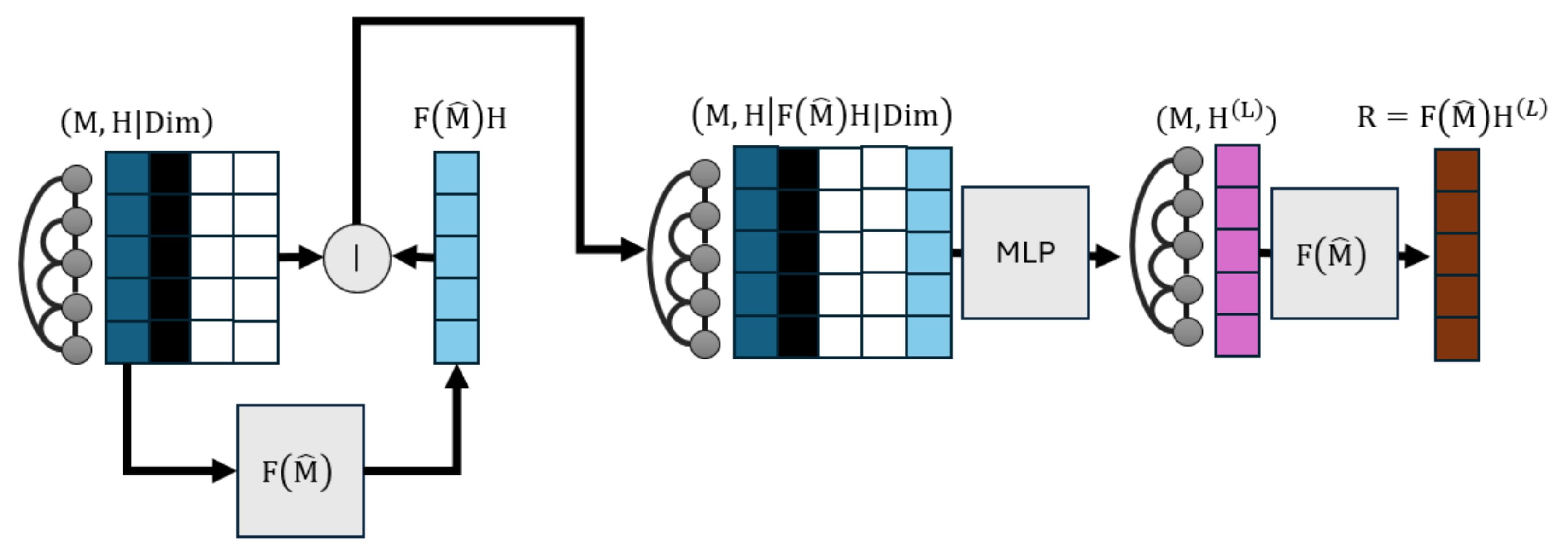
Figure 5.
The ULA architecture pipeline based on its one-dimensional counterpart (ULA1D in Figure 4) that produces posteriors given prior representations . The priors are unwrapped into a vector, and concatenated with an embedding of features dimension identifiers that each unwrapped row is retrieved from. Unwrapping also creates repetitions of the graph into a larger adjacency matrix with M as its block diagonal elements. Outputs are rewrapped into matrix form. Linear layers change the dimensions of node feature at the beginning and and of outputs at the end.
4.1. Multidimensional Universal Attraction
First, we tackle the problem of multiple node feature dimensions to be diffused. Our strategy involves treating each node feature dimension as a separate graph signal defined on copies of the graph stacked together in a supergraph. We then optimize all dimensions by creating a supergraph of them. This also creates a signal that stacks all dimensions on top of each other. The methodology of this section is similar to the proof of Lemma 3 in that it vertically concatenates representations and creates an underlying supergraph. However, if we blindly performed an unwrapping of tensor H to an one-dimensional counterpart holding all its information, any computed loss function would not be symmetric with respect to feature dimensions, as different dimensions require different outputs. This would mean that computations would not be invariant with respect to node features, as a permutation of features would create a different loss for different nodes.
To address this issue, we look back at Theorem 1, which stipulates that all necessary information to compute the loss should be included as columns of H. In our case, the necessary information consists of which feature dimension identifiers (i.e., the column numbers of H) each entry corresponds to. We can capture this either via an one-hot encoding or via an embedding representation; we opt for the second approach to avoid adding too many new dimensions to the one-dimensional unwrapped H; it suffices to learn or fewer embedding dimensions for . Mathematically:
where is the ULA1D architecture, ; is vertical concatenation that vertically unwraps the representation matrix H, | is horizontal concatenation, is a matrix of zeroes of appropriate dimension, is a matrix of ones, and a trainable embedding mechanism from integer identifiers to a matrix. To understand this formula, are matrices that vertically repeat the corresponding embeddings times to differentiate the feature dimension each row refers to. The concatenated result has dimensions where is the number of nodes in the new supergraph.
We now make use of ULA1D’s theoretical properties to generate posteriors R that locally minimize the loss for every attributed graph . If the loss is equivariant, it is equivalent to defining an equivariant loss in terms of given an re-wrapping of R to matrix with K columns:
for vectors . We do not need additional theoretical analysis to show that any loss can be approximated, given that we reshaped how matrices are represented while leaving all computations the same and that therefore Theorems 1 and 2 still hold.
4.2. Different Node Feature and Prediction Dimensions
As a last step in designing our architecture, we introduce two additional layers as the first and last steps. In the former, we transform input features X to lower-dimensional representations of dimension that promote a computationally tractable architecture (Section 4.3). The output linear layer also maps from K representation dimensions to output dimensions.
Considering that R (and, equivalently, ) is the outcome of the intermediate ULA1D that guarantees local attractiveness, the input and output transformation components are essentially part of the loss minimized by the ULA1D architecture of Equation 3. In particular, a loss function defined over ULA’s multidimensional outputs Y is equivalent to minimizing the loss:
where , and and are the input and output transformations respectively. To enable an immediate application of local attractiveness results, the new loss needs to still have Lipschitz gradients, which in turn means that input and output transformations should not be able to approximate arbitrary functions, i.e., they cannot be MLPs. Furthermore, the input transformation needs to be invertible. Selecting both transformations as linear layers and setting satisfies both properties. For ease of implementation, we make transformation trainable, but they may also be extrapolated from informed ad-hoc strategies, like node embeddings for matrix factorization.
4.3. Implementation Details
Implementations of the ULA architecture should take care to follow a couple of points requisite for either theoretical analysis or common machine learning principles to apply. Ignoring any of these suggestions may cause ULA to get stuck at shallow local minima:
- a.
- The output of ULA1D should be divided by 2 when the parameter initialization strategy of relu-activated layers is applied everywhere. This is needed to preserve input-output variance, given that there is an additional linear layer on top. This is not a hyperparameter. Contrary to the partial robustness to different variances exhibited by typical neural networks, having different variances between the input and output may mean that the original output starts from “bad” local minima, from which it may even fail to escape. In the implementation we experiment with later, failing to perform this division makes training get stuck near the architecture’s initialization.
- b.
- Dropout can only be applied before the output’s linear transformation. We recognize that dropout is a necessary requirement for architectures to generalize well, but it cannot be applied on input features due to the sparsity of the representation, and it cannot be applied on the transformation due to breaking any (approximate) invertibility that is being learned.
- c.
- Address the issue of dying neurons for ULA1D. Due to the few feature dimensions of this architecture, it is likely for all activations to become zero and make the architecture stop learning from certain samples from the beginning of training with randomly initialized parameters. In this work, we address this issue by employing leaky relu as the activation function in place of . This change does not violate universal approximation results that we enlist. Per Theorem 3, activation functions should remain Lipschitz and have Lipschitz derivatives almost everywhere; both properties are satisfied by .
- d.
- Adopt a late stopping training strategy that repeats training epochs until both train and validation losses do not decrease for a number of epochs. This strategy lets training overcome saddle points where ULA creates a small derivative. For a more thorough discussion of this phenomenon refer to Section 6.2.
- e.
- Retain linear input and output transformations, and do not apply feature dropout. We previously mentioned the necessity of the first stipulation, but the second is also needed to maintain Lipschitz loss derivatives for the internal ULA1D architecture.
4.4. Running Time and Memory
In Appendix C we analyse the proposed architecture’s running time and memory consumption in big-O complexity notation. These are:
where N is the number of the graph filter’s parameters, and the number of hidden node feature dimensions. Both complexities grow slightly worse than linearly as we choose more hidden dimensions, but our architecture remains computationally tractable; it is worse than linear increase by a logarithmic scale on a well-controlled quantity, and incomparable to the exponential increase in compute that would be needed to add more tensor dimensions, as happens for GNNs satisfying univeral approximation.
Still, in terms of absolute orders of magnitute the logarithmic scale inside running time analysis is ; for selected in experiments there is a 6-fold increase in running time and memory compared to simply running an APPNP architecture for graph diffusion. Factoring in that propagation through graph filters runs twice (once to get initial posteriors, and then to refine them again) and we obtain an approximate factor of 12-fold increase in running time compare to APPNP. This means that large graphs residing at the limits of existing computing resources could be hard to process with ULA. Still, our architecture runs faster and consumes less memory than GCNII of those we compare with in Section 5.2.
In experiments, we employ GPUs that let us parallelize feature dimensions, and hence reduce the number of hidden dimension multiplications from to for the purposes of running time analysis. That is, the running time complexity under this parallelization is divided by K. Performant implementation of sparse matrix multiplication is not achievable by existing GPU frameworks, and for graphs with few enough nodes that can fit the adjacency matrix in GPU memory we prefer dense matrices and corresponding operations. In this case, instead of diffusion requiring computations it should be substituted with in the above complexities. We also adopt this to speed up experiments given that we train hundreds of architectures for hundreds of training epochs each, but in larger graphs the sparse computational model is both faster and more memory-efficient.
5. Experiments
In this section we use ULA to approximate various AGFs, and compare it against several popular architectures. In Appendix D we show that ULA can be represented with an appropriate MPNN; it essentially adds constraints to which parameter combinations can be learned to satisfy the local attraction property. Consequently, our architecture’s expressive power is at most WL-1 and we compare it with well-performing alternatives of at most as much expressive power described in Section 5.2. We also perform an investigative comparison against an MPNN enriched with random node representations for greater expressive power. Tasks we experiment on are described in Section 5.1, and span graph analysis algorithms and node classification. Experimentation code is based on PyTorch Geometric [30], and is available online as open source.4 We conduct all experiments on a machine with 16GB RAM and 6GB GPU memory.
5.1. Tasks
For our evaluation, we created a collection of synthetic and real-world tasks. Of these, synthetic tasks present various degrees of expressive power and difficulty in being optimized by GNN architectures (including ULA). Each comprises a set of a 500 synethetically generated graphs of uniformly chosen numbers of nodes. There is a uniformly random chance of linking each pair of nodes, with an added line path across all nodes in each graph to make them connected. The tasks we compute for these graphs are the following, where 4Clique and LongShort require more than WL-1 expressive power to be densely approximated:
- Degree. Learning to count the number of neighbors of each node. Nodes are provided with an one-hot encoding of their identifiers within the graph, which is a non-equivariant input that architectures need to learn to transfer to equivariant objectives. We do not experiment with variations (e.g., other types of nodes encodings) that are promising for the improvement of predictive efficacy, as this is a basic go-to strategy and our goal is not—in this work— to find the best architectures but instead assess local attractiveness. To simplify experiment setup, we converted this discretized task into a classification one, where node degrees are the known classes.
- Triangle. Learning to count the number of triangles. Similarly to before, nodes are provided with an one-hot encoding of their identifiers within the graph, and we convert this discretized task into a classification one, where the node degrees observed in the training set are the known classes.
- 4Clique. Learning to identify whether each node belongs to a clique of at least four members. Similarly to before, nodes are provided with an one-hot encoding of their identifiers within the graph. Detecting instead of counting cliques yields a comparable number of nodes between the positive and negative outcome, so as to avoid complicating assessment that would need to account for class imbalances. We further improve class balance with a uniformly random number of chance of linking nodes. Due to the high computational complexity of creating the training dataset, we restrict this task only to graphs with a uniformly random number of nodes.
- LongShort. Learning the length of the longest among shortest paths from each node to all others. Similarly to before, nodes are provided with an one-hot encoding of their identifiers within the graph, and we convert this discretized task into a classification one, where path lengths in training data are the known classes.
- Propagate. This task aims to relearn the classification of an APPNP architecture with randomly initialized weights and uniformly random (the same for all graphs) that is applied on nodes with 16 feature dimensions, uniformly random features in the range and 4 output classes. This task effectively assesses our ability to reproduce a graph algorithm. It is harder than the node classification settings bellow in that features are continuous.
- 0.9Propagate. This is the same as the previous task with fixed . Essentially, this is perfectly replicable by APPNP, which means that that any failure of the latter to find deep minima for it should be attributed to the need for better optimization strategies.
- Diffuse. This is the same task as above, with the difference that the aim to directly replicate output scores in the range for each of the 4 output dimensions (these are not soft-maximized).
- 0.9Diffuse. This is the same as the previous task with fixed . Similarly to 0.9Propagate, this task is in theory perfectly replicable by APPNP.
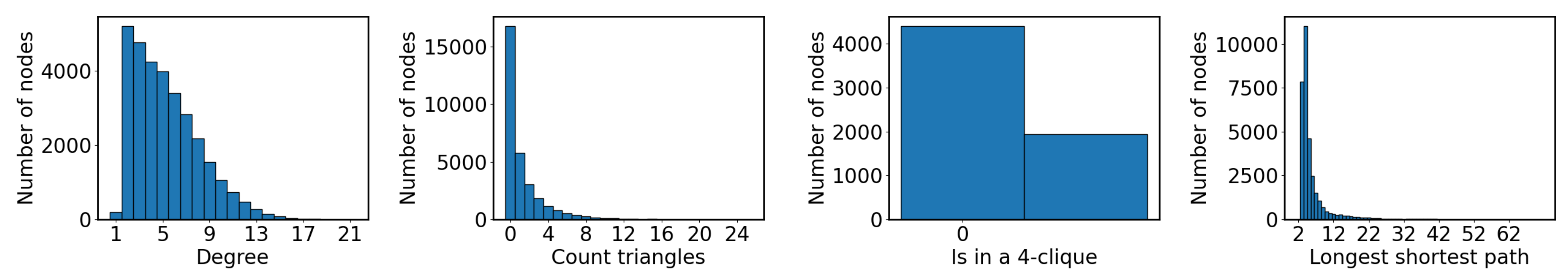
Figure 6.
Distributions (in that order) of degrees, triangle counts, existence of 4-cliques, and longest shortest path distances in synthetic graphs.
Figure 6.
Distributions (in that order) of degrees, triangle counts, existence of 4-cliques, and longest shortest path distances in synthetic graphs.
In addition to the above, we also conduct node inference experiments across the following three real-world attributed graphs. These are used for the evaluation of GNNs for node classification, and we point out that they run on only one graph. In general, WL-1 architectures are accepted as the best-performing on these datasets, as there is no need to distinguish between different graphs:
- Cora [31]. A graph that comprises nodes and edges. Its nodes exhibit feature dimensions and are classified in one among 7 classes.
- Citeseer [32]. A graph that comprises nodes and edges. Its nodes exhibit feature dimensions and are classified in one among 6 classes.
- Pubmed [33]. A graph that comprises nodes and edges. Its nodes exhibit 500 feature dimensions and are classified iin one among 3 classes.
5.2. Compared Architectures
We select architectures that are conceptually similar to ours in that they employ graph diffusion mechanisms. All experimented architectures are MPNNs, which means that they exhibit at most WL-1 expressive power. Therefore we may safely attribute differences in predictive efficacy as the hardness of optimizing them.
- MLP. A two-layer perceptron that does not leverage any graph information. We use this as a baseline to measure the success of graph learning.
- GAT [13]. A gated attention network that learns to construct edge weights based on the representations at each edge’s ends, and uses the weights to aggregate neighbor representations.
- GCNII [34]. An attempt to create a deeper variation of GCN that is explicitly design to be able to replicate the diffusion processes of graph filters, if needed. We employ the variation with 64 layers.
- APPNP [8]. The predict-then-propagate architecture with ppr base filter. Switching to different filters lets this approach maintain roughly similar performance, and we opt for its usage due to it being a standard player in GNN evaluation methodologies.
- ULA [this work]. Our universal local minimizer presented in this work. Motivated by the success of APPNP on node classification tasks, we also adopt the first 10 iterations of personalized PageRank as the filter of choice, and leave further improvements by tuning the filter to future work.
Additionally, we compare our approach with one of greater expressive power:
- GCNNRI. This is the GCN-like MPNN introduced by Abboud et al. [24]; it employs random node representations to admit greater (universal approximation) expressive power and serves as a state-of-the-art baseline. We adopt its publicly available implementation, which first transforms features through two GCN layers of Equation 2 and concatenates them with a feature matrix of equal dimensions sampled anew in each forward pass. Afterwards, GCNNRI applies three more GCN layers and then another three-layered MLP. The original architecture max-pooled node-level predictions before the last MLP to create an invariant output (i.e., one prediction for each graph), but we do not do so to accommodate our experiment settings by retaining equivariance, and therefore create a separate prediction for each node. We employ the variation that replace half of node feature dimensions with random representations.
5.3. Evaluation Methodology
Training process. For synthetically generated datasets, we create a -- train-validation-test split across graphs, of which training and validation graphs are respectively used to train the architecture, and to avoid overtraining by selecting parameters with minimal validation loss. For real-world graphs, we create an evaluation split that avoids class imbalance in the training set, and for this reason we perform stratified sampling to obtain 50, 50 validation, and 100 test nodes. In all settings, training epochs repeat until neither training nor validation loss decrease for a patience of 100 consecutive epochs. We retain parameter values corresponding to the best validation loss.5 For classification tasks, including counting tasks where the output is an integer, the loss function is categorical cross-entropy after applying softmax activation on each architecture’s outputs. For regression tasks, the loss function is the mean absolute error.
Predictive performance. For all settings, we measure either accuracy (acc—larger is better) or mean absolute error (mabs—smaller is better) and compute their average across 5 experiment repetitions. We report these quantities instead of the loss because we aim to create practically useful architectures that can accurately approximate a wide range of AGF objectives. Evaluation that directly considers loss function values is even more favorable for our approach (see Section 6), though of limited practical usefulness. Since we are making a comparison between several architectures, we also compute Nemenyi ranks; for each experiment repetition, we rank architectures based on which is better (rank 1 is the best, rank 2 the second best, and so on) and average these across each task’s repetition, and afterwards across all tasks. In the end, we employ the Friedman test to reject the null hypothesis that architectures are the same at the p-value level, and then check for statistically significant differences at the p-value level between every architecture and ULA with the two-tailed Bonferroni-Dunn test [35], which Demsar [36] sets up as a stronger variation of the Nemenyi test [37]. For our results of comparisons and 7 compared methods, the test has critically difference rounded up; rank differences of this or greater value are considered statistically significant. We employ the Bonferroni-Dunn test because it is both strong and easy to intuitively understand.
Assessing minimization capabilities. To check whether we succeed in our main goal of finding deep minima, we also replicate experiments by equalizing training, validation, and test sets and investigating how well architectures can replicate the AGFs they are meant to reproduce. That is, we investigate the ability of architectures to either overtrain, as this is a key property of universal approximation, or -failing that- to univerally minimize objectives. Notice that success in this type of evaluation (i.e., success in overtraining) is the property we are mainly interested in this work, as it remains an open question for GNNs, contrary to traditional neural networks for which it is well-established. We measure predictive performance above only to get a sense of how well the learned AGFs generalize.
Hyperparameter selection. To maintain a fair comparison between compared architectures, we employ the same hyperparameters for the same conceptually similar choices by repeating common defaults across GNN literature. In particular, we use the same number of 64 output dimensions for each trained linear layer, and dropout rate for node features and for all outputs of 64-layer representations except for ULA’s input and output layers (which do not accept dropout). For GAT, we use the number of attention heads tuned on the Cora dataset, which is 8. All architectures are also trained using the Adam optimizer with learning rate (this is the commonly accepted default for GNNs) and default other parameters. For all other choices, like diffusion rates, we defer to architecture defaults.We initialize dense parameters with Kaiming initilization [38]. Due to already high computational demands, we did not perform extensive hyperparameter tuning, other than a simple verification that statistically singificant changes could not be induced for both the Degree and Cora tasks (we selected these as conceptually simple) by modifying parameters or injecting or removing layers, and in Section 6.4 we explain why this is not a substantial threat to the validity of evaluation outcomes.
5.4. Experiment Results
Table Table 2 summarizes experiment results across all tasks. In the case of generalization, ULA remains close to the best-performing architectures, which vary across experiments. This corroborates its universal minimization property, i.e., minimizing a wide breadth of objectives. There are certain tasks in which our approach is not the best, but this can be attributed to intrinsic shortcomings of cross-entropy as a loss function that at best approximates accuracy; even in cases where accuracy was not the highest, losses were smaller during experimentation (Section 6.1). Even better, experiment results reveal that ULA successfully finds deep local minima, as indicated by its very ability to overtrain, something which other architectures are not always capable of.
A somewhat unexpected finding is that ULA outperforms GCNNRI in almost all experiments despite the significantly worse theoretical expressive power. We do not necessarily expect this outcome to persist across all real-world tasks and experiment repetitions, but it clearly indicates that (universal) local attraction may be a property far more useful than universal approximation. Overall, the Friedman test asserts that at least one approach is different than the rest, and differences between ULA and all other architectures are statistically significant by the Bonferroni-Dunn test when all tasks are considered, both when generalizing and when attempting to overtrain.
From high-level point of view, we argue that there is no meaning to devising GNNs with rich expressive power without also accompanying training strategies that can unlock that power. For example, ULA exhibiting imperfect but over 95% accuracy in overtrained node classification on one graph could be an upper limit for our approach’s expressive power, but it is a limit that is henceforth known to be achievable. Furthermore, overtrained ULA, and in some cases GCN and GCNNRI, outperform overtrained MLP on these tasks, where the latter essentially identifies node based on their features, which reflects its ability to leverage the the graph structure for finding deeper minima. Another example of expressive power not being the limiting factor of predictive performance is that APPNP is always outperformed by ULA—and often by other architectures too—in the 0.9Diffusion and 0.9Propagation tasks, despite theoretically modeling them with exact precision (the two tasks use APPNP itself to generate node scores and labels respectively).
6. Discussion
In this section we discuss various aspects of ULA with respect to its practical viability. In Section 6.1 we observe that our architecture being occasionally outperformed by other methods stems from the gap between accuracy and usage of the categorical cross-entropy loss for training; ULA always finds deeper local optima for the latter. Then, in Section 6.2 we describe the convergence speed and observe the existence of groking phenomena that are needed to escape from shallow local minima. Finally, in Section 6.3 we summarize the mild requirements needed for practical usage of ULA, and in Section 6.4 we point out threats to this work’s validity.
6.1. Limitations of Cross-Entropy
In the generalization portion of Table 2, ULA is not always the best-performing architecture. This happens because, when minimization reaches minima of similarly low loss values, other architectures incorporate implicit assumptions about the form of the final predictions that effectively regularize it to a favorable choice. For example, the smoothness constraint imposed by APPNP and GCNII layers often establish them as the most accurate methods for the node classification datasets, which are strongly homophilic (i.e., when neighbors tend to have similar labels). This happens at the cost of the same assumptions drastically failing to induce deep minima in other tasks. Therefore, there is still merit in architectures curated for specific types of problems, as these may be enriched with hypotheses that let shallows losses generalize better. On the other hand, ULA should be preferred for solving unknown (black box) problems. Experimental validation is still required though, because expressive power is also a limiting factor of our approach and hard problems could require a lot of data and architecture parameters to train (Section 6.4 includes a more in-depth discussion of this concern).
Even when ULA is not the best approach, accuracy differences with the best approach are small and—importantly—we empirically verified that it still finds deeper minima for the optimized loss functions. For example, in Table 3 we show train, validation, and test losses and accuracies of all trained architectures in a Cora experiment (at the point where best validation loss is achieved) and the minimum train loss achieved throughout training; ULA indeed finds the deepest validation loss minimum. Thus, the lesser predictive ability compared to alternatives comes both from differences between validation and test losses, and discrepancy between minimizing the cross-entropy loss and actual accuracy.
It is standard practice to employ categorical cross-entropy as a loss function in lieu of other accuracy maximization objectives, as a differentiable relaxation. However, based on our findings, following the same practice for node classification, at least for inductive learning with a few number of samples, warrants further investigation. For example, adversarial variations of the loss function could help improve generalization to true accuracy when classification outcome is not too certain. Finally, MLP being able to reach relative deep losses on the train but not on valid or test splits is an indication that node features can largely reconstruct node labels, but the way to do so should be dependent on the graph structure.
6.2. Convergence Speed and Late Stopping
Universal attraction creates regions of small gradient values. However, some of these could form around saddle points through which optimization trajectories pass. These could also be shallow local minima that optimization strategies like Adam’s momentum can overcome. To let learning strategies overcome such phenomena, in this work we train GNNs by employing a late stopping criterion. In this, we stop training only if neither training nor validation loss has decreased for a set number of epochs, called the patience. Early stopping at the point where validation losses no longer decrease with a patience of 100 epochs is already standard practice in GNN literature, but in this work we employ late stopping with the same patience to make a fair comparison between architectures by not underestimating the efficacy of the literature.
Late stopping comes at the cost of additional computational demands, as training takes place over more (e.g., a couple of thousand instead of a couple of hundred) epochs. However, in Figure 7 we demonstrate that this practice is necessary, at least for ULA, by investigating the progress of losses in the first of the LongShort experiments; there is a shallow loss plateau early on that spans hundreds of epochs, in which early stopping may have erroneously halted training.
6.3. Requirements to Apply ULA
Here we summarize the conditions needed to employ ULA in new settings while benefiting from its local attraction property. We consider these mild in that they are already satisfied by many settings. In addition to checking these conditions in new settings, make sure to follow necessary implementation details of Section 4.3, as we do in our publicly available implementation at the experiment repository.
- a.
- The first condition is that processes graphs should be unweighted and undirected. Normalizing adjacency matrices is accepted (we do this in experiments—in fact it is necessary to obtain the spectral graph filters we work with), but structurally isomorphic graphs should obtain the same edge weights after normalization. Otherwise, Theorem 3 cannot hold in its present form. Future theoretical analysis can consider discretizing edge weights to obtain more powerful results.
- b.
- Furthermore, loss functions and output activations should be twice differentiable and each of their gradient dimensions Lipschitz. Our results can be easily extended to differentiable losses with continuous non-infinite gradients by framing their linearization needed by Theorem 1 as a locally Lipschitz derivative. However, more rigorous analysis is needed to extend results to non-differentiable losses, even to those that are differentiable “almost everywhere”.
- c.
- Lipschitz continuity of loss and activation derivatives is typically easy to satisfy, as any Lipschitz constant is acceptable. That said, higher constant values will be harder to train, as they will require more finegrained discretization. Notice that the output activation is considered part of the loss in our analysis, which may simplify matters. Characteristically, passing softmax activation through a categorical cross-entropy loss is known to create gradients equal to the difference between predictions and true labels, which is a 1-Lipschitz function and therefore accepts ULA. Importantly, having no activation with mabs or L2 loss is admissible in regression strategies, for example because the L2 loss has a 1-Lipschitz derivative, but using higher powers of score differences or KL-divergence is not acceptable, as their second derivatives are unbounded and thus not Lipschitz.
- d.
- Finally, ULA admits powerful minimization strategies but requires positional encodings to exhibit stronger expressive power. To this end, we suggest following progress on respective literature.
6.4. Threats to Validity
Before closing this work, we point to threats to validity that future researcher based on this work should account for. To begin with, we introduced local attraction as a property that induces deep loss minima thanks to allowing training losses to escape from shallow local minima. This claim is a hypothesis that we did not verify through analysis; results discussed above, like ULA’s efficicacy in finding smaller loss values in all cases and the groking behavior, align with our hypothesis. However, it also requires theoretical justification that we left for future work. For example, further investigation is needed between our objective of creating plateaus and how valleys and or local maxima are affected. We reiterate the importance of this work as a first demonstration that GNNs with the local attraction property actually exist.
In terms of experimental validation, we did not perform hyperparameter tuning due to the broad range of experiment settings we visited. This is a threat to interpreting exact assessment values of provided architectures, as improved alternatives could exist. However, our main point of interest was to understand substantial qualitative differences between architectures that can not be bridged by hyperparameter tuning. For example, ULA exhibits close to double the predictive accuracy compared to the similarly powerful GCN in some tasks of Table Table 2. When applying the same common defaults on hyperparameter values, we also verified that minor adjustments (including adding additional layers) did not improve predictive efficacy for the Degree and Cora settings by any noticeable amount, but more principled exploration can be conducted by benchmarking papers.
Choosing paper defaults could err in favor overestimating the abilities of existing GNNs on the non-synthetic graphs in that we select only architecturs and parameters that are both tuned and known to work well. We employ this practice because it does not raise concerns over our approach’s viability, and given that computationally intensive experimentation is needed to tune hyperparameters in all settings.
Finally, experiment results were evaluated on synthetic graphs with a small number 100 of nodes (up to 500), mainly due to computational constraints of larger-scale experimentation. This number of graphs was empirically selected as sufficient for small predictive differences between training and validation sets across all experiments. For graphs with more nodes, ULA could require a non-polynomial number of hidden layer dimensions, as this was an intermediate step in our proofs. Thus, for harder tasks and without sufficient training data or number of parameters, other architectures could reach deeper minima. Furthermore, we can not necessarily extrapolate efficacy to an unbounded number of nodes because theoretical results do not hold in that scenario; at the very least include graphs with the number of nodes that will be seen in practice to validation set. Finally, if an insufficient number of training samples is provided, overtraining—even with validation precautions—persists as a risk that should be investigated for an approach tailored to deep minimization.
7. Conclusions and Future Directions
In this work we introduced the local minimization property as a means of creating GNN architectures that can find deep minima of loss functions, even when they can not express the best fit. We then created the ULA architecture that refines the predict-then-propagate scheme to become a local attractor for a wide range of losses. We experimentally corroborated that this architecture can find deep local minima in a collection of several tasks compared to architectures of similar or greater expressive power. Thus, local attraction and, in general, properties that improve the deepness of learned minima warrant closer scrutiny by the literature, especially when it is difficult to make assumptions about the predictive task (e.g., whether it can be best supported by homophilous diffusion) are not known a-priori and universally promising options are sought out.
Future works need to properly analyze the benefits of local attraction beyond the empirical understanding gleaned from our experiments. In particular, our results can combined with optimization theory and loss landscape analysis results of traditional neural networks [3]. Furthermore, local attractors with controlled attraction areas could serve as an alternatives to GNN architecture search [39]. Furthermore, ULA could be combined with architectures with greater expressive power, especially FPGNN [15], which exhibits WL-3 and while also applying MLPs on all node feature dimensions. Moreover, concerns over a potentially large breadth or width of intermediate layers can be met by devising mechanisms that create (coarse) invariant representations of each graph’s structure. Finally, compatibility or trade-offs between universal AGF approximation and local attractiveness should be investigated.
Author Contributions
Conceptualization, Emmanouil Krasanakis and Symeon Papadopoulos; Data curation, Emmanouil Krasanakis; Formal analysis, Emmanouil Krasanakis; Funding acquisition, Symeon Papadopoulos and Ioannis Kompatsiaris; Investigation, Emmanouil Krasanakis; Methodology, Emmanouil Krasanakis; Project administration, Symeon Papadopoulos and Ioannis Kompatsiaris; Resources, Symeon Papadopoulos and Ioannis Kompatsiaris; Software, Emmanouil Krasanakis; Supervision, Symeon Papadopoulos; Validation, Emmanouil Krasanakis, Symeon Papadopoulos and Ioannis Kompatsiaris; Visualization, Emmanouil Krasanakis; Writing – original draft, Emmanouil Krasanakis; Writing – review & editing, Symeon Papadopoulos.
Funding
This work and the APC was partially funded by the European Commission under contract number H2020-951911 AI4Media, and by the European Union under the Horizon Europe MAMMOth project, Grant Agreement ID: 101070285. UK participant in Horizon Europe Project MAMMOth is supported by UKRI grant number 10041914 (Trilateral Research LTD).
Data Availability Statement
Experiments, datasets, and implemented architectures can be found online at: https://github.com/MKLab-ITI/ugnn.
Conflicts of Interest
The authors declare a conflict of interest with regards to the Centre for Research & Technology Hellas: Employment.
Appendix A. Terminology
For the sake of completeness, in this appendix we briefly describe several properties that we mention in the course of this work.
Boundedness. This is a property of quantities that admit a fixed upper numerical bound, matrices whose elements are bounded, or functions that output bounded values.
Closure. Closed sets are those that include all their limiting points. For example, a real-valued closed that contains open intervals also includes their limit points .
Compactness. We use the sequential definition of compactness, for which compact sets are closed and bounded.
Connectivity. This is a property of sets cannot be divided into two disjoint non-empty open subsets. Equivalently, all continuous functions from connected sets to are constant.
Density. In the text we often claim that a space A is dense in a set B. The spaces often contain functions, in which case we consider a metric the worst deviation under any input, which sets up density as the universal approximation property of being able to find members of A that lie arbitrarily close to any desired elements of B.
Lipshitz continuity. We refer to multivariate multivalue functions as c-Lipshitz if they satisfy the property for some chosen p-norm . Throughout this work, we consider this property for the norm , which computes the maximum of absolute values. If a Lipshitz function is differentiable, then it is c-Lipshitz only if . If two functions are Lipshitz, their composition and sum are also Lipshitz. If they are additionally bounded, their product is also Lipshitz.
Appendix B. Theoretical Proofs
Lemma 1.
For a positive definite graph filter and differentiable loss over graph signal domain , update graph signals over time per:
where are the smallest positive and largest eigenvalues of respectively. This leads to if posteriors remain closed in the domain, i.e., if .
Proof.
For non-negative posteriors , and non-zero loss gradients, the Cauchy-Shwartz inequality in the bilinear space determined by the positive definite graph filter yields:
where is the matrix transposition symbol. Therefore, the loss asymptotically converges to a locally minimum point. □
Lemma 2.
Let a differentiable graph signal generation function6 on compact connected domain Θ admit some parameters such that . If, for any parameters , the Jacobian has linearly independent rows (each row corresponds to a node) and satisfies:
then there exist parameters such that .
Proof.
Let us consider a differentiable trajectory for parameters for times that starts from and (asymptotically) arrives at some . For this trajectory, it holds that . Let us also consider the posteriors arising from the graph signal generation function at times t for parameters , as well the least square problem of minimizing the projection of the loss’s gradient to the row space of :
The closed form solution to this problem can be found by:
Thus, as long as (we will call this Proposition P.I), this lemma’s first precondition can be written for posteriors and as:
We now set as the derivatives of some parameters across their trajectory, that is:
Therefore, from Lemma 1 we obtain that our system asymptotically arrives at locally optimal posteriors, i.e., with for .
As a final step, we now investigate the priors signal editing converges at. To do this, we can see that the update rule leads to the selection of priors at times t for which:
For some parameters . We can similarly show that Proposition P.I holds true. Hence, there exists an optimization path of prior editing parameters (not necessarily the same as the one followed by the optimization algorithm used in practice) that arrives at the edited priors that let posteriors exhibit local optimality. □
Theorem 1.
Take the setting of Lemma 2, where the loss’s Hessian matrix linearly approximates the gradients within the domain with error at most . Let us construct a node feature matrix whose columns are graph signals (its rows correspond to nodes v). If , , and all graph signals other than r involved in the calculation of are columns of , and it holds that:
for any , then for any there exists with relu activation, for which
Proof.
Let be the Hessian matrix of with respect to node values of the graph signal of a domain . Given that its rank is , there exists a decomposition with fixed inner dimensions . That is, has dimensions and has dimensions where counts the dimensions of the parameter space (i.e., is the number of parameters). When , the decomposition even becomes unique for the particular r.
We now select a prior generation model with linearly independent rows and a Jacobian that is a function (e.g., an MLP) approximating well the first of the decomposition elements. That is, for any chosen small enough but non-negligible constant within the domain it holds that:
Throughout this proof, r is a function of , but we do not write for simplicity. The Jacobian does not need to have linearly independent rows; small perturbations (with cumulative effect that, when added to the actual approximation error, makes it smaller than ) can be injected in each row to make the rows of its approximation linearly independent. Additionally, we use the Hessian as a linear estimator of gradients per:
We now rewrite the loss’s gradient as a linear transformation of a factor with an error term :
where the factor is , and the error term admits a small bound:
At this point, we choose , which yields
Applying the linear estimation obtained above on the quantities of Lemma 2 we obtain:
However, the matrix is indempondent (that is, it holds ) and therefore its eigenvalues are either 0 or 1. Thus:
Given that we showed the existence of a (deep neural network) function, , we integrate it to retrieve and then approximate the integral with a new deep neural network. Given the universal approximation theorem’s form described by [26] the latter can be the architecture described by this theorem, used to produce error less than . In this case:
We could not immediately assume the existence of that final network, because we needed to verify that the Jacobian’s properties for the function it approximates and “hide” methods of tracking equal partial derivatives of different nodes behind the term .
As a final remark, one of the preconditions for Lemma 2’s application is for posteriors r to remain within the domain enclosing . Effectively, this stipulates that is implicitly injected into the loss function as a choice on which direction to follow. One way to achieve this is demonstrated in Theorem 2. □
Theorem 2.
There exists sufficiently large parameter for which
satisfies the properties needed by Theorem 1 within the following domain:
where is the ideal posteriors optimizing the regularized loss. If the second term of the max is selected, it suffices to have no regularization .
Proof.
For ease of notation, during this proof we define . Without loss of generality, consider to be a twice differentiable closure of the sign function on the optimization trajectory, i.e., a tight enough approximation of the element-by-element sign operator. If and are the maximum derivative approximation error of and respectively, it suffices to select such that:
where the first case needs to come alongside the condition
but in the second case it suffices to select any . Given an appropriate selection, we obtain the necessary criterion:
□
Lemma 3.
Let a finite set of attributed graphs with undirected unweighted adjacency matrices M with up to a finite number of nodes v and one-dimensional node representations H be denoted as . Let loss be twice diffentiable with respect to r and any . Then any selected that lets Equation 3 be local loss minimum on all attributed graphs of is contained in a connected neighborhood of for which:
Proof.
Let us write and create the block-diagonal matrix:
and the feature matrix , where ; is the vertical concatenation symbol (don’t forget that this lemma refers to the one-dimensional setting where are vectors, and therefore H is also a vector.
By Theorem 2, the ULA1D architecture of Equation 3 admits parameters that reproduce gradient norm up to for any twice differentiable loss, including the loss such that
It also holds that:
given that adjacency normalization is considers only row and column degrees for each node, and potentially adding self-loops that add the unit matrix on the diagonal. Given this result, we now concatenate vertically all parts of our predictive pipeline to obtain that: . Thus, for any element i of , we obtain:
As a final remark, we stress that previous theoretical results were obtained for a finite number of nodes, and for this reason this proof only works on a set with a finite number of elements, which set up M as the adjacency matrix of a graph with a finite number of nodes (the sum of all nodes in the set of graphs). Handling an infinite number of graphs is tackled in the proof of Theorem 3 that follows. □
Theorem 3.
Consider infinite sets , bounded node feature values, Lipshitz loss gradients with respect to both h and r, and that has activation functions that are almost everywhere Lipshitz with Lipshitz derivatives (e.g., relu). Then, Lemma 3 holds for a dense subset of the neighborhood.
Proof.
Our chosen is -Lipshitz with respect to H for some value , as it is composed from Lipshitz functions (activations and linear matrix multiplications and additions). Consider that has a -Lipshitz derivative. We can now write:
where obtains the maximum absolute value of vector elements. Similarly, for the quantity
is -Lipshitz with respect to for some constant , i.e., . Note that above all loses have as the second argument. We also have that the quantity
is -Lipshitz with respect to for some constant , i.e.,
.
At the same time, consider the discretization of the feature space H that creates a collection for numerical precision whose exact value will be selected later on:
For the discretization it holds that, for every and there exists the closest element in , for which:
Having established bounds for the error of replacing elements of with their discretized equivalents, we now move on to the main proof. Consider any , select a fixed with appropriate value (we will see how to determine this later). Now, the discretization has a number of elements upper bounded by a finite number:
where is a finite number due to bounded feature values, i.e., it is the maximum difference of values across all feature dimensions. Therefore, per Lemma 3 there exists compact domain around with more than one elements for which given that . From this we obtain that, for any in a new connected subset (this new set still has more than two elements and is compact and connected as an interesection of compact and connected sets):
where the last equality holds for the choice . As a final remark, is -Lipschitz almost everywhere, given that it is is composed by a finite number of almost-everywhere Lipschitz derivatives. Therefore, there exists a subset of that is dense on the latter, for which -Lipschitz. Thus, our choice for exists and is finite, because the denominator is positive and is finite, which in turn holds true given that is compact and the L2 norm continuous. □
Appendix C. Algorithmic Complexity
Let us annotate the embedding dimension and entertain a scenario with no parallelization. The generation time of embedding matrix is proportional to its number of elements and therefore . Linear node feature transformations also require time and the output linear layer requires time . Inside ULA1D, for sparse matrix-vector multiplication on each filter parameter we require time:
assuming that self-loops are added, so that , where L is the number of the employed filter’s parameters and is the number of nodes of the base graph, i.e., the number of non-zero elements of the adjacency metric M and not of . This is because we perform a premature re-wrapping of into vector form (this is just a computational rearrangement) before passing it through the filter , effectively going back to left-multiplying each feature dimension with the normalized adjacency matrix.
However, MLP layers within ULA1D multiply the combined graph attributes with dense transformations with parameter dimensions, and the outcome of the latter with dense transformation of dimensions (since is a column matrix). This requires total time . In the end, summing all these running times, we obtain the following time needed to run one forward pass:
In terms of memory complexity, for graph filter propagation we iteratively compute matrices for all by left-multiplying the outcome for with an aggregate them into one matrix with the same dimensions of . This requires memory that is independent of N, and becomes given that ULA1G parses nodes with dimensions each. Additionally, we need to store adjacency matrices in memory, and layer parameters that similarly to before consume at worst memory for ULA1D. Input and output linear transformations consume and memory respectively. Overall, summing these requirements we have the following memory needs:
Appendix D. ULA as an MPNN
Here we explain that any trained ULA architecture can be written as an MPNN. To begin with, both MLPs and propagation of node representation matrices one hop away constitute message passing layers. For example, predict-then-propagate architectures like APPNP are also MPNNs. At the same time, passing the unwrapped H through an MLP is equivalent to passing through a different MLP’ the wrapped version holding the same values:
for corresponding layer representations with MPNN layers:
where and . In this variation, the rewrapped version of is equal to .
References
- Loukas, A. What graph neural networks cannot learn: Depth vs width. arXiv arXiv:1907.03199 2019.
- Nguyen, Q.; Mukkamala, M.C.; Hein, M. On the loss landscape of a class of deep neural networks with no bad local valleys. arXiv arXiv:1809.10749 2018.
- Sun, R.Y. Optimization for deep learning: An overview. Journal of the Operations Research Society of China 2020, 8, 249–294. [Google Scholar] [CrossRef]
- Bae, K.; Ryu, H.; Shin, H. Does Adam optimizer keep close to the optimal point? arXiv arXiv:1911.00289 2019.
- Ortega, A.; Frossard, P.; Kovačević, J.; Moura, J.M.; Vandergheynst, P. Graph signal processing: Overview, challenges, and applications. Proceedings of the IEEE 2018, 106, 808–828. [Google Scholar] [CrossRef]
- Page, L.; Brin, S.; Motwani, R.; Winograd, T.; et al. The pagerank citation ranking: Bringing order to the web 1999.
- Chung, F. The heat kernel as the pagerank of a graph. Proceedings of the National Academy of Sciences 2007, 104, 19735–19740. [Google Scholar] [CrossRef]
- Gasteiger, J.; Bojchevski, A.; Günnemann, S. Predict then propagate: Graph neural networks meet personalized pagerank. arXiv, arXiv:1810.05997 2018.
- Agarap, A.F. Deep learning using rectified linear units (relu). arXiv, arXiv:1803.08375 2018.
- Gilmer, J.; Schoenholz, S.S.; Riley, P.F.; Vinyals, O.; Dahl, G.E. Neural message passing for quantum chemistry. In Proceedings of the International conference on machine learning. PMLR; 2017; pp. 1263–1272. [Google Scholar]
- Balcilar, M.; Héroux, P.; Gauzere, B.; Vasseur, P.; Adam, S.; Honeine, P. Breaking the limits of message passing graph neural networks. In Proceedings of the International Conference on Machine Learning. PMLR; 2021; pp. 599–608. [Google Scholar]
- Kipf, T.N.; Welling, M. Semi-supervised classification with graph convolutional networks. arXiv arXiv:1609.02907 2016.
- Velickovic, P.; Cucurull, G.; Casanova, A.; Romero, A.; Lio, P.; Bengio, Y.; et al. Graph attention networks. stat 2017, 1050, 10–48550. [Google Scholar]
- Cai, J.Y.; Fürer, M.; Immerman, N. An optimal lower bound on the number of variables for graph identification. Combinatorica 1992, 12, 389–410. [Google Scholar] [CrossRef]
- Maron, H.; Ben-Hamu, H.; Serviansky, H.; Lipman, Y. Provably powerful graph networks. Advances in neural information processing systems 2019, 32. [Google Scholar]
- Morris, C.; Ritzert, M.; Fey, M.; Hamilton, W.L.; Lenssen, J.E.; Rattan, G.; Grohe, M. Weisfeiler and leman go neural: Higher-order graph neural networks. In Proceedings of the Proceedings of the AAAI conference on artificial intelligence, 2019, Vol. 33, pp. 4602–4609.
- Zaheer, M.; Kottur, S.; Ravanbakhsh, S.; Poczos, B.; Salakhutdinov, R.R.; Smola, A.J. Deep sets. Advances in neural information processing systems 2017, 30. [Google Scholar]
- Keriven, N.; Peyré, G. Universal invariant and equivariant graph neural networks. Advances in Neural Information Processing Systems 2019, 32. [Google Scholar]
- Maron, H.; Fetaya, E.; Segol, N.; Lipman, Y. On the universality of invariant networks. In Proceedings of the International conference on machine learning. PMLR; 2019; pp. 4363–4371. [Google Scholar]
- Xu, K.; Hu, W.; Leskovec, J.; Jegelka, S. How powerful are graph neural networks? arXiv arXiv:1810.00826 2018.
- Wang, H.; Yin, H.; Zhang, M.; Li, P. Equivariant and stable positional encoding for more powerful graph neural networks. arXiv arXiv:2203.00199 2022.
- Keriven, N.; Vaiter, S. What functions can Graph Neural Networks compute on random graphs? The role of Positional Encoding. Advances in Neural Information Processing Systems 2024, 36. [Google Scholar]
- Sato, R.; Yamada, M.; Kashima, H. Random features strengthen graph neural networks. In Proceedings of the 2021 SIAM international conference on data mining (SDM). SIAM, 2021; pp. 333–341.
- Abboud, R.; Ceylan, I.I.; Grohe, M.; Lukasiewicz, T. The surprising power of graph neural networks with random node initialization. arXiv arXiv:2010.01179 2020.
- Krasanakis, E.; Papadopoulos, S.; Kompatsiaris, I. Applying fairness constraints on graph node ranks under personalization bias. In Proceedings of the Complex Networks & Their Applications IX: Volume 2, Proceedings of the Ninth International Conference on Complex Networks and Their Applications COMPLEX NETWORKS 2020. Springer, 2021, pp. 610–622.
- Kidger, P.; Lyons, T. Universal approximation with deep narrow networks. In Proceedings of the Conference on learning theory. PMLR; 2020; pp. 2306–2327. [Google Scholar]
- Hoang, N.; Maehara, T.; Murata, T. Revisiting graph neural networks: Graph filtering perspective. In Proceedings of the 2020 25th International Conference on Pattern Recognition (ICPR). IEEE; 2021; pp. 8376–8383. [Google Scholar]
- Huang, Q.; He, H.; Singh, A.; Lim, S.N.; Benson, A.R. Combining Label Propagation and Simple Models Out-performs Graph Neural Networks. arXiv arXiv:2010.13993 2020.
- Zhou, D.; Bousquet, O.; Lal, T.; Weston, J.; Schölkopf, B. Learning with local and global consistency. Advances in neural information processing systems 2003, 16. [Google Scholar]
- Fey, M.; Lenssen, J.E. Fast graph representation learning with PyTorch Geometric. arXiv arXiv:1903.02428 2019.
- Bojchevski, A.; Günnemann, S. Deep gaussian embedding of graphs: Unsupervised inductive learning via ranking. arXiv arXiv:1707.03815 2017.
- Sen, P.; Namata, G.; Bilgic, M.; Getoor, L.; Galligher, B.; Eliassi-Rad, T. Collective classification in network data. AI magazine 2008, 29, 93. [Google Scholar] [CrossRef]
- Namata, G.; London, B.; Getoor, L.; Huang, B.; Edu, U. Query-driven active surveying for collective classification. In Proceedings of the 10th international workshop on mining and learning with graphs; 2012; Volume 8, p. 1. [Google Scholar]
- Chen, M.; Wei, Z.; Huang, Z.; Ding, B.; Li, Y. Simple and deep graph convolutional networks. In Proceedings of the International conference on machine learning. PMLR; 2020; pp. 1725–1735. [Google Scholar]
- Dunn, O.J. Multiple comparisons among means. Journal of the American statistical association 1961, 56, 52–64. [Google Scholar] [CrossRef]
- Demšar, J. Statistical comparisons of classifiers over multiple data sets. The Journal of Machine learning research 2006, 7, 1–30. [Google Scholar]
- Hollander, M.; Wolfe, D.A.; Chicken, E. Nonparametric statistical methods; John Wiley & Sons, 2013.
- He, K.; Zhang, X.; Ren, S.; Sun, J. Delving deep into rectifiers: Surpassing human-level performance on imagenet classification. In Proceedings of the IEEE international conference on computer vision, 2015; pp. 1026–1034.
- Nunes, M.; Fraga, P.M.; Pappa, G.L. Fitness landscape analysis of graph neural network architecture search spaces. In Proceedings of the Genetic and Evolutionary Computation Conference, 2021; pp. 876–884.
| 1 | If we replaced GNNs with independent optimization for each node when only one graph is analysed, we would not be able to impose structural properties that let the predictive performance generalize to validation and test data; this is demonstrated by experiment results for the MLP architecture in Section 5. |
| 2 | In Lemma 2, the subscript is the function’s input. |
| 3 | Larger radii can be obtained for near-quadratic objectives, for which is small. In practice, this can be imposed by also adding a large enough L2 regularization, but we leave theoretical study of this option to future work. |
| 4 | |
| 5 | We allow decreases in training losses to reset the stopping patience in order to prevent architectures from getting stuck at shallow minima, especially at the beginning of training. This increases the training time of architectures to requiring up to 6,000 epochs in some settings, but in return tends to find much deeper minima when convergence is slower. A related discussion is presented in Section 6.2. |
| 6 | In Lemma 2, the subscript is the function’s input. |
Figure 1.
Different types of minima for a loss of one-dimensional prediction r of one data sample.
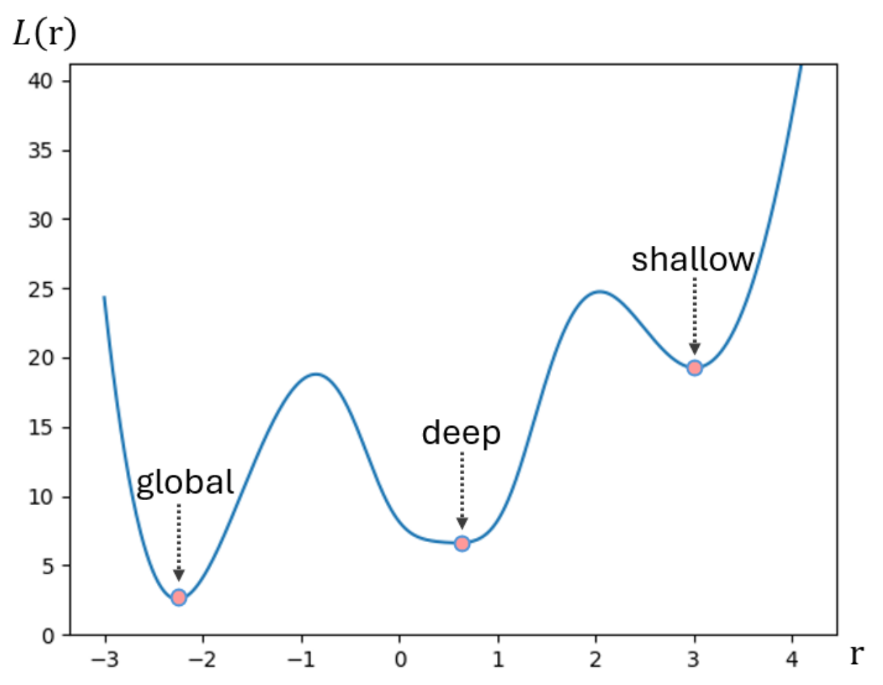
Figure 2.
Landscape of a loss for values of pairwise linked nodes produced for and ideal selection of z (left), and landscape of the same loss produced by a GNN architecture (right), where are trainable parameters and are column vectors.
Figure 2.
Landscape of a loss for values of pairwise linked nodes produced for and ideal selection of z (left), and landscape of the same loss produced by a GNN architecture (right), where are trainable parameters and are column vectors.
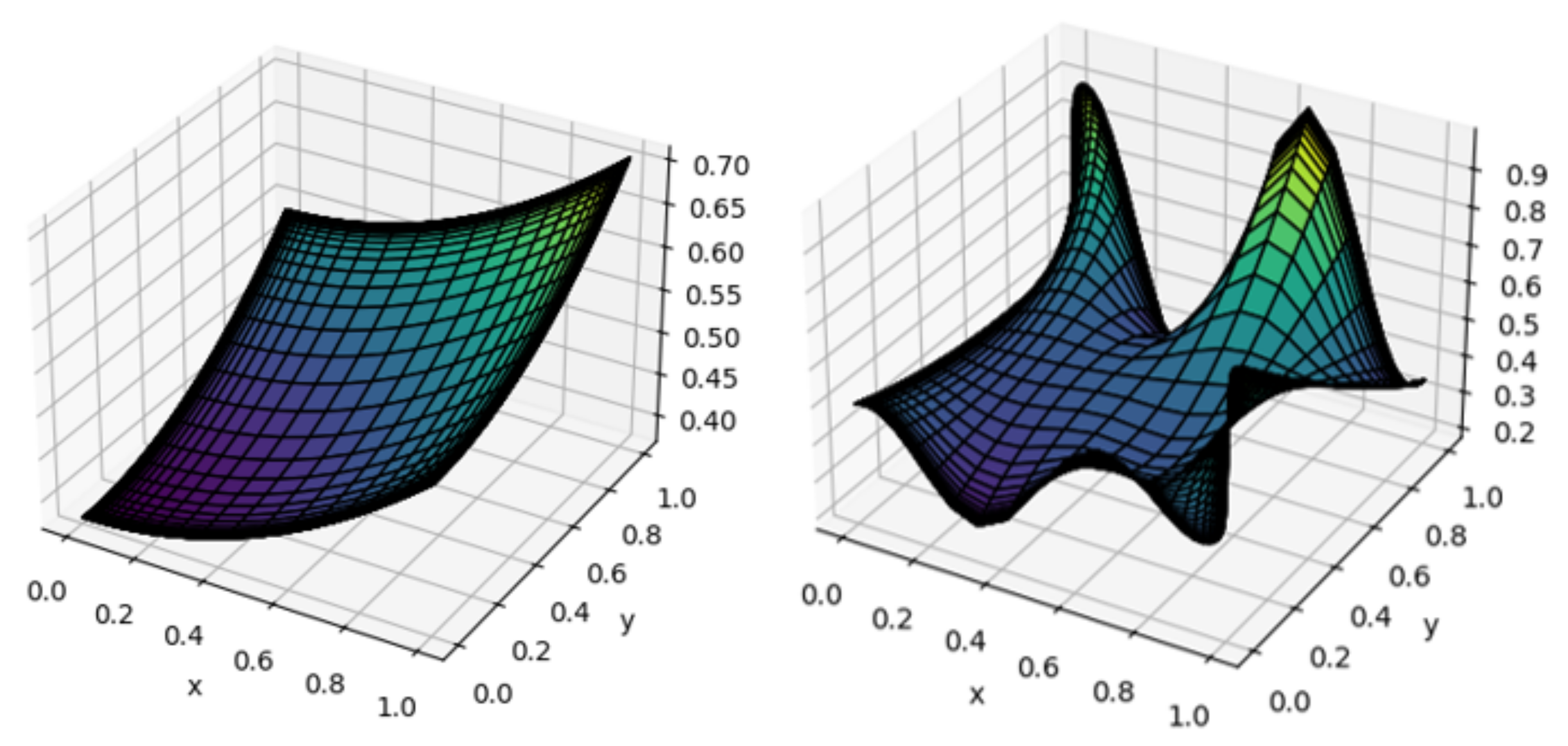
Figure 3.
Two non-isomorphic graphs that can be distinguished by FWL-2 but not by WL-1 or WL-2.
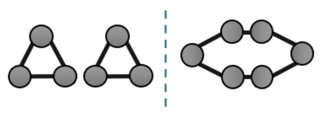
Figure 7.
Convergence of train, validation, and test set losses of ULA (left) and GCNRNI (right).
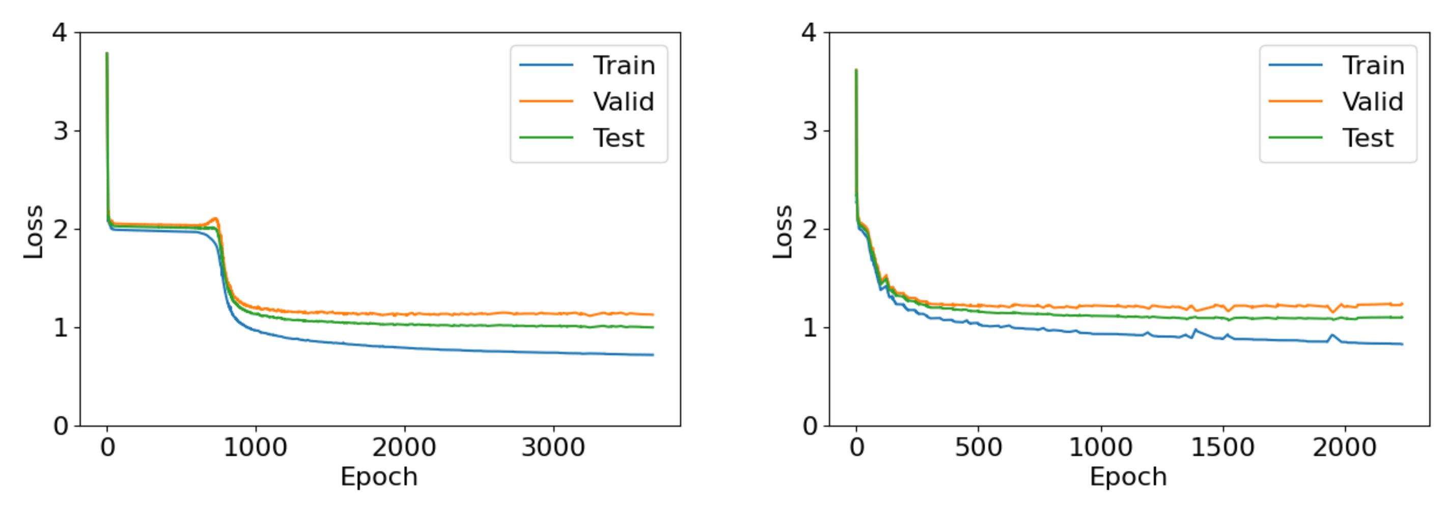
Table 2.
Evaluations of predictive performance and their Nemenyi ranks in parentheses across 5 repetitions of each task. For each task, best performance is in bold.
Table 2.
Evaluations of predictive performance and their Nemenyi ranks in parentheses across 5 repetitions of each task. For each task, best performance is in bold.
| Task | Eval. | MLP | GCN [12] | APPNP [8] | GAT [13] | GCNII [34] | GCNNRI [24] | ULA |
|---|---|---|---|---|---|---|---|---|
| Generalization | ||||||||
| Degree | acc ↑ | 0.162 (5.6) | 0.293 (2.8) | 0.160 (6.2) | 0.166 (5.6) | 0.174 (4.6) | 0.473 (2.0) | 0.541 (1.2) |
| Triangle | acc ↑ | 0.522 (5.2) | 0.523 (3.6) | 0.522 (5.2) | 0.522 (5.2) | 0.522 (5.2) | 0.554 (2.4) | 0.568 (1.2) |
| 4Clique | acc ↑ | 0.678 (4.9) | 0.708 (4.1) | 0.677 (6.2) | 0.678 (4.9) | 0.678 (4.9) | 0.846 (2.0) | 0.870 (1.0) |
| LongShort | acc ↑ | 0.347 (5.8) | 0.399 (3.0) | 0.344 (6.4) | 0.350 (4.2) | 0.348 (5.6) | 0.597 (2.0) | 0.653 (1.0) |
| Diffuse | mabs ↓ | 0.035 (4.0) | 0.032 (2.8) | 0.067 (7.0) | 0.035 (5.0) | 0.037 (6.0) | 0.030 (2.2) | 0.012 (1.0) |
| 0.9Diffuse | mabs ↓ | 0.021 (4.6) | 0.015 (3.0) | 0.034 (7.0) | 0.021 (4.4) | 0.021 (6.0) | 0.009 (1.8) | 0.007 (1.2) |
| Propagate | acc ↑ | 0.531 (2.6) | 0.501 (4.0) | 0.510 (3.6) | 0.455 (6.1) | 0.443 (6.9) | 0.503 (3.8) | 0.861 (1.0) |
| 0.9Propagate | acc ↑ | 0.436 (5.3) | 0.503 (3.0) | 0.452 (4.0) | 0.418 (5.8) | 0.401 (6.7) | 0.546 (2.2) | 0.846 (1.0) |
| Cora | acc ↑ | 0.683 (6.6) | 0.855 (4.2) | 0.866 (1.4) | 0.850 (4.1) | 0.863 (2.4) | 0.696 (6.4) | 0.859 (2.9) |
| Citeseer | acc ↑ | 0.594 (6.0) | 0.663 (3.9) | 0.676 (2.3) | 0.661 (4.0) | 0.679 (1.8) | 0.443 (7.0) | 0.669 (3.0) |
| Pubmed | acc ↑ | 0.778 (6.4) | 0.825 (3.7) | 0.835 (2.0) | 0.821 (4.0) | 0.835 (2.1) | 0.747 (6.6) | 0.829 (3.2) |
| Average (CD=1.1) | (5.2) | (3.5) | (4.7) | (4.8) | (4.7) | (3.5) | (1.6) | |
| Deepness (overtraining capability) | ||||||||
| Degree | acc ↑ | 0.172 (5.7) | 0.331 (3.0) | 0.170 (6.6) | 0.175 (5.7) | 0.186 (4.0) | 0.632 (1.2) | 0.571 (1.8) |
| Triangle | acc ↑ | 0.510 (4.7) | 0.510 (4.2) | 0.510 (4.7) | 0.510 (4.7) | 0.510 (4.7) | 0.536 (3.8) | 0.568 (1.2) |
| 4Clique | acc ↑ | 0.665 (5.0) | 0.779 (3.0) | 0.657 (6.4) | 0.665 (5.0) | 0.663 (5.6) | 0.898 (1.4) | 0.894 (1.6) |
| LongShort | acc ↑ | 0.347 (6.0) | 0.391 (3.0) | 0.347 (6.0) | 0.351 (4.0) | 0.347 (6.0) | 0.588 (2.0) | 0.688 (1.0) |
| Diffuse | mabs ↓ | 0.032 (4.4) | 0.028 (3.0) | 0.061 (7.0) | 0.032 (4.6) | 0.033 (6.0) | 0.026 (2.0) | 0.012 (1.0) |
| 0.9Diffuse | mabs ↓ | 0.021 (4.6) | 0.015 (3.0) | 0.034 (7.0) | 0.021 (4.4) | 0.021 (6.0) | 0.009 (1.8) | 0.007 (1.2) |
| Propagate | acc ↑ | 0.477 (4.2) | 0.502 (2.4) | 0.454 (4.4) | 0.461 (4.9) | 0.413 (6.6) | 0.503 (4.5) | 0.844 (1.0) |
| 0.9Propagate | acc ↑ | 0.493 (4.8) | 0.527 (2.8) | 0.534 (3.2) | 0.444 (6.3) | 0.451 (6.5) | 0.534 (3.4) | 0.873 (1.0) |
| Cora | acc ↑ | 0.905 (5.6) | 0.914 (3.2) | 0.905 (5.4) | 0.911 (3.8) | 0.864 (7.0) | 0.930 (2.0) | 0.996 (1.0) |
| Citeseer | acc ↑ | 0.865 (2.2) | 0.818 (3.8) | 0.794 (6.0) | 0.808 (5.0) | 0.767 (7.0) | 0.849 (3.0) | 0.959 (1.0) |
| Pubmed | acc ↑ | 0.868 (3.8) | 0.871 (2.0) | 0.862 (5.2) | 0.855 (6.8) | 0.859 (6.0) | 0.869 (3.2) | 0.956 (1.0) |
| Average (CD=1.1) | (4.2) | (3.0) | (5.6) | (5.0) | (6.0) | (2.6) | (1.2) | |
Table 3.
Differences between accuracy maximization and categorical cross-entropy minimization on one Cora experiment. The best value of each column is in bold.
Table 3.
Differences between accuracy maximization and categorical cross-entropy minimization on one Cora experiment. The best value of each column is in bold.
| loss (↓) | acc (↑) | |||||
|---|---|---|---|---|---|---|
| Train | Valid | Test | Train | Valid | Test | |
| MLP | 0.113 (min 0.103) | 1.061 | 1.059 | 1.000 | 0.657 | 0.659 |
| GCN | 0.198 (min 0.194) | 0.541 | 0.564 | 0.986 | 0.863 | 0.860 |
| APPNP | 0.288 (min 0.284) | 0.544 | 0.563 | 0.971 | 0.869 | 0.860 |
| GAT | 0.261 (min 0.254) | 0.546 | 0.574 | 0.983 | 0.866 | 0.854 |
| GCNII | 0.425 (min 0.423) | 0.656 | 0.668 | 0.951 | 0.866 | 0.849 |
| GCNNRI | 0.262 (min 0.015) | 0.839 | 0.936 | 0.929 | 0.789 | 0.759 |
| ULA | 0.161 (min 0.007) | 0.479 | 0.890 | 0.974 | 0.854 | 0.846 |
Disclaimer/Publisher’s Note: The statements, opinions and data contained in all publications are solely those of the individual author(s) and contributor(s) and not of MDPI and/or the editor(s). MDPI and/or the editor(s) disclaim responsibility for any injury to people or property resulting from any ideas, methods, instructions or products referred to in the content. |
© 2024 by the authors. Licensee MDPI, Basel, Switzerland. This article is an open access article distributed under the terms and conditions of the Creative Commons Attribution (CC BY) license (http://creativecommons.org/licenses/by/4.0/).
Copyright: This open access article is published under a Creative Commons CC BY 4.0 license, which permit the free download, distribution, and reuse, provided that the author and preprint are cited in any reuse.


