
Submitted:
18 April 2024
Posted:
18 April 2024
You are already at the latest version
Abstract
In this paper, the entire downhole fluid sucker rod pump system is replaced with a viscoelastic vibration model, namely a third-order differential equation with an inhomogeneous forcing term. Both Kelvin and Maxwell viscoelastic models can be implemented along with the dynamic behaviors of a mass point attached to the viscoelastic model. By employing the time-dependent polished rod force measured with a dynamometer as the input to the viscoelastic dynamic model, we have obtained the displacement responses, which match closely with the experimental measurements in actual operations, through an iterative process. The key discovery of this work is the feasibility of the so-called inverse optimization procedure which can be utilized to identify the equivalent scaling factor and viscoelastic system parameters. The proposed Newton-Raphson iterative method with some terms in the Jacobian matrix expressed with averaged rates of changes based on perturbations of up to two independent parameters provides a feasible tool for optimization issues related to complex engineering problems with mere information of input and output data from either experiments or comprehensive simulations. The same inverse optimization procedure is also implemented to model the entire fluid delivery system of a very viscous non-Newtonian polymer modeled as a first-order ordinary differential system similar to the transient entrance developing flow. The convergent parameter reproduces transient solutions which match very well with those from full-fledged computational fluid dynamics models with the required inlet volume flow rate and the outlet pressure conditions.
Keywords:
inverse
; optimization
; viscoelastic
; computation
Towards the end of typical petroleum reservoir’s productive life, natural lift force due to fluid pressure tends to decay and diminish. Thus, it is common to use artificial lift methods to transfer the oil and gas from the underground formation to the surface [1,2,3]. Sucker rod pumping systems, as the most popular artificial lift means, are widely utilized along with hydraulic and electric submersible pumping system [4,5,6,7]. Teaming with such pumping systems, various four-bar linkage based horse-head pump jacks have also been invented to support and to drive the entire artificial lift system [31]. As one of the earliest inventions for oil industries, these sucker rod pump systems have been proved to be efficient and adaptable [8,9,10,11,29]. Over of the wells worldwide still depend on this traditional and most extensively used mechanism [12,13]. Nevertheless, contemporary computational tools have been introduced in recent research efforts on leakage, safety, and reliability and shed light on these popular artificial lift systems [14,15,18,19].
The so-called relaxation time which can be derived numerically based on the Bessel function of the first kind and the second kind for cylindrical coordinates and Fourier series for Cartesian coordinates, is confirmed to be less than a tenth of the typical sampling period, which corresponds to a sampling frequency, normally ranging from 30 to 60 samples per second, used in oil industries with comparable physical dimensions [20,32]. The issues related to the leakage also exposed an imminent desire and need in engineering practice that sophisticated perturbation methods and analytical approaches continue to be essential to derive information from full-fledge computational simulations and, in some cases, to help the establishment of viable and more insightful simulation setups [21,22,23,24,25,26,27]. In fact, through the exercises of applying full-fledged computational fluid dynamics (CFD) and finite element method (FEM) to sucker rod pump systems, it is becoming clear that even for a simple developing viscous fluid within sucker rod pump systems with extreme aspect ratios, for example, the the so-called clearance, namely, the difference between the outer diameter of the plunger and the inner diameter of the barrel, is often measured in mills, one-thousandth of an inch, whereas, the plunger system length is often measured in feet [16,17,30]. To follow up with the ideas reported in Ref. [28], in which the entire downhole sucker rod pump systems are modeled with Kelvin or Maxwell viscoelastic systems, in this paper, we focus more on the iterative procedure to identify the optimal choice of needed parameters in these models with a so-called Inversed Optimization Method. The preliminary results do confirm that the parameters derived with the Inversed Optimization Method yield virtually identical results in comparison with the dynamometer measurement of the polished rod load and the displacement in the field, which consists of a moving contact area between the traveling unit (plunger), a chamber with a so-called traveling valve, and the tube or barrel with a so-called standing valve [29,33,34]. The same inverse optimization procedure is also implemented to model the entire fluid delivery system of a very viscous non-Newtonian polymer as a mere first-order ordinary differential system. The convergent parameter matches very well with that identified with the full-fledged computational fluid dynamics model with the required pressure drop as the input and the flow rate as the output.
1. Theory and Modeling
Let’s consider a lumped mass linked with either Maxwell or Kelvin models as illustrated in Figure 1. A sudden displacement is applied to the Maxwell model whereas a sudden load is introduced to the Kelvin model [28]. Consequently, the Maxwell model will yield a stiffness function or relaxation function to relate the responding force with the sudden imposed displacement as shown in Figure 2. Likewise, the Kelvin model will produce a compliance function or creep function to relate the resulting displacement with the suddenly imposed force also shown in Figure 2. For the Maxwell model, we also introduce the displacement where is the Heaviside function. The total force function can be expressed as the combination of the location force and for the stiffness and dashpot couple with the relaxation time . Furthermore, using the same force or stress for the series component and the same displacement or strain for the parallel component, we obtain the following governing equations for the Maxwell model:
Hence, using the concepts we have been discussing for the first-order ODE, we obtain:
namely, by using integration by parts,
Finally, we have and the total force for the Maxwell model. Likewise, denote the sudden load as where is a Heaviside function, the total displacement function can be expressed as the combination of the location displacement and for the stiffness and dashpot couple with the relaxation time . Using the same force or stress for the series component and the same displacement or strain for the parallel component, we obtain the following governing equations for the Kelvin model:
Thus, using the concepts we have been discussing for the first-order ODE, we obtain:
Finally we have the local displacement and the total displacement function can be expressed as for the Kelvin model. To further the discussion with relaxation and creep functions, we can also introduce a general Kelvin viscoelastic model as elaborated in Ref. [35]. Similar approaches are also implemented for the viscoelastic vibration model with a mass m and a concentrated load . We introduce first the Kelvin viscoelastic model in a dynamic case as shown in Figure 9, essentially a typical Kelvin viscoelastic setup for creep test combined in series with a spring with a stiffness k and a mass m. The displacement of the parallel section of the stiffness and the dashpot share the same displacement , whereas the displacement of the stiffness k is denoted as . Since the mass m is connected with the stiffness k in series, the total displacement of the mass is a combination of the two displacements and . In general, the external load is applied to the mass m. We can imagine that in the creep test, we can simply add a dead weight in addition to the weight of the mass .
Use the same procedure, consider each section in series and the consequent continuity of axial forces, we have
Using the kinematic relationship , we obtain the following third-order governing equation for ,
In this paper, for simplicity, in the implementation of the inverse optimization approaches, Eq. (9) is directly applied with adjusted parameters k, m, , and . The measured force is introduced to derive the closest which matches with the measured displacement. As validated in Ref. [28], with no dashpot, namely, , Eq. (8) yields
hence
Finally, the governing equation (9) yields the familiar spring-mass vibration system
Notice the effective stiffness of two springs in series. Moreover, the infinitely stiff spring k, namely, , consequently, and . Finally, we recover the familiar spring-mass-dashpot vibration system
Finally, in order to facilitate the solution, introduce the state variable , we can rewrite the third-order viscoelastic vibration system with a dynamical system format,
Let’s consider the Maxwell viscoelastic model in a dynamic case as shown in Figure 9, essentially a typical Maxwell viscoelastic setup for relaxation test combined a mass m connecting in series with two parallel branches, one with a stiffness k and another one with a stiffness and a dashpot in series. The displacement of the parallel section shares the same displacement , whereas the displacement of the stiffness is denoted as and the dashpot as . Since the displacement of the stiffness k is , naturally, the total displacement of the mass is a combination of the two displacements and within one of the parallel branches. In general, the external load is applied to the mass m. We can imagine that in a relaxation test, we can simply add a dead weight in addition to the weight of the mass . Using the same procedure, assuming the force in the dashpot and stiffness series as , consider each section in series and the consequent continuity of axial forces, we have
Using the kinematic relationship as well as , we obtain the following third-order governing equation for ,
Again, with no dashpot, namely, . Equation (8) yields , hence the governing equation (11) yields the familiar spring-mass vibration system
Likewise, as the infinitely stiff spring , namely, , consequently, and we recover the familiar spring-mass-dashpot vibration system
As presented in Ref. [28], in numerical solutions, we rewrite the third-order viscoelastic vibration system with a dynamical system format,
with the state variable , and
As shown in Figure 3 and Figure 4, for such a viscoelastic model representing the down-hole sucker rod system and starting from the zero position with zero velocity and zero acceleration, we employ , , , , and . The external force is a deadweight . Based on the Matlab simulation, it is clear that the vibration eventually settles down to an equilibrium position due to the dashpot damping. Of course, we will replace the deadweight with the actual dynamometer load measurements and compare the displacement solutions with the actual polish rod displacements. As shown in Figure 5, even with a very preliminary Kelvin model, we can still recreate the hysteresis loop of load and displacement for the sucker rod pump system. In the simulation, the magnification factor is 85 for both Maxwell and Kelvin models to match the actual motion of the sucker rod with the viscoelastic model in the simulation. Notice that the load used in the viscoelastic model is the exact load measurement recorded in TAM software examples. In general, by reducing the parameter m, the peak of the displacement will decrease and shift to the left which corresponds to the increase of the natural frequency. In addition, the end point will also decrease accordingly. Moreover, by reducing the parameter k, the peak of the displacement will increase and the end point will also be elevated accordingly. By increasing the parameter , the viscous damping is increased and both the displacement peak and the ending points will be increased. Finally, by increasing the stiffness parameter , both the displacement peak and the end displacement tend to decrease. Notice that here the magnification factor C along with the parameters m, , and are chosen with intuition through trial and error methods and human interventions as reported in Ref. [28]. However, in this paper, with the initial guesses of these parameters, we will implement a so-called Inversed Optimization Method to identify with iterations in the steepest decents the optimal set of parameters. With this Newton-Raphson iteration-based approach, these parameters will be searched and improved automatically. An improvement Kelvin viscoelastic vibration system with adjusted parameters m, , and demonstrates a much closer displacement response with the measured force as shown in Figure 5, which demonstrates the potential of inverse optimization approaches with the Newton-Raphson iterations.
2. Inverse Optimization
In engineering practice, there are many complex systems that are impossible to characterize with a simple physical and mathematical model, therefore, an implicit matrix-free iterative method is very useful in providing better guidance to the optimum operation conditions with only the availability of the input and output data. The inverse optimization based on the Newton-Raphson iterations can be used to search more strategically for the optimal system parameters. It can be used to search without knowing the true relationship between the optimal material compositions to achieve the best mechanical properties or any type of property. Of course, similar acceleration methods commonly employed in the Newton-Raphson iterations can also be available for the design of more efficient and purposeful search processes.
In inverse optimization approaches, in order to identify these intrinsic viscoelastic properties with the consideration of different physical units, we also introduce a scaling factor C. We set up an inverse engineering problem to minimize the difference measured by the following variational indicator
where N represents the number of time stations, is the displacement evaluated with the viscoelastic model with the stiffness k, m, , and , whereas is the experimental measurement of the displacement in question at the same time intervals. For the minimized error, cost function, or variational indicator E, we have
This estimate evaluated with finite difference schemes will be directly coupled with the system parameters, for example, k, m, , and ,
It is clear that we must introduce the Newton-Raphson iterative procedures to obtain the solution of the nonlinear and implicit set of equations. In general, the Newton-Raphson iterative method should be used for this type of nonlinear set of equations. The nonlinear and implicit governing equation about the unknown vector , can be rewritten as
where the given right-hand side vector .
It is very important to point out that the initial guess must be fairly close to the actual solution for the unknown to ensure the convergence of the Newton-Raphson iteration scheme. In practice, we often start with a few tryouts and narrow down the true solution neighborhood. With an educated guess of the initial set of parameters , not too far from the converged solution, the Jacobian matrix can be defined and evaluated. Assume we have all the information before the iteration, namely, and the corresponding as well as the so-called Jacobian matrix with all entities defined as
Furthermore, the off-diagonal terms for the Jacobian matrix with can also be elaborated as
It is straightforward to confirm that the Jacobian matrix is indeed symmetric. After the solution of the following incremental linear system of equations for the unknown
with the following update,
The iteration identified in Eq. (15) will stop with the relative incremental error smaller than prescribed small number ,
In the actual implementation, since we do not the analytical expressions for , , , and , a central-difference-based numerical scheme is introduced. Assume the increment , we will complete the numerical integration of the dynamic response of the viscoelastic model for three sets of parameters, namely, , , , and obtain the numerically the approximations as follows
As the most complicated term, the second partial derivative with respect to and with , namely, is evaluated as follows
In the implementation, we can always use a sufficiently small increment for the partial derivatives of as a function of .
3. Implementation and Improvement
In order to verify this proposed inverse optimization procedure, we start with a simple first-order differential equation with one parameter, a so-called relaxation time , expressed as
where is a time dependent inhomogenous term.
Instead of the actual experimental measurement, in the validation process, we employ the actual analytical solution , expressed as
with the initial solution and the convolution term with the so-called Green’s function for impulse
Note that although we have the analytical solution as a continuous function, in engineering practice, the experimental measurements often exist in discrete form. Therefore, a proper number of time steps N must be taken before we start the inverse optimization process for the search of the system parameter which yields the solution with In the initial implementation, the maximum number of iterations is set to be 200 and the time station number is 2001. In addition, the finite difference approximation of some of the implicit terms of the Jacobian matrix is based on the perturbation of the parameter and the scaling factor C. The analytical solution is based on the relaxation time . As shown in Table 1, the only system parameter, namely the relaxation time , does converge to a value very close to 5 within approximately range. Moreover, the scaling factor C is also simultaneously converged to 1. The quadratic convergence rate towards the end of the iteration processes is evident in Table 1.
It is well accepted that there is no guarantee for the Newton-Raphson iteration to converge in particular when the initial guess is very far away from the desired solution. Moreover, it is often possible that different initial solutions will lead to different branches of solutions [35,36]. Different acceleration procedures have been proposed to improve the convergence behaviors of these nonlinear iterative solution procedures such as line search methods [37]. In this paper, based on the understanding of the possible solution key features, we can also start the optimization procedure from the very beginning. For example, for the first-order ordinary differential equation exponential solutions, rather than connection with the solution itself, we can choose to connect with the logarithmic of the solution. In this way, the nonlinear system can be less challenging which can fundamentally change the basin of convergence in the Newton-Raphson iterative procedures. Hence, we set up an inverse engineering problem to minimize the difference measured by the following variational indicator
where N represents the number of time stations, is the displacement evaluated with the system parameter, in this case, the relaxation time , is the experimental measurement of the displacement in question at the same time intervals, and D stands for the new constant which is related to the initial scaling factor C with .
Similarly, to the minimized error, cost function, or variational indicator E, we have
Note that the scaling constant D still has an explicit expression, the derivative with respect to D will be evaluated directly unlike the system parameter which must be evaluated with finite difference schemes. This estimate of the scaling factor D will be directly coupled with the system parameter and form the unknown vector with , with the nonlinear set of equations expressed as
In order to effectively carry out the Newton-Raphson iterative procedures for the nonlinear and implicit governing equation about the unknown vector , the so-called Jacobian matrix must be properly evaluated,
Furthermore, the off-diagonal terms for the Jacobian matrix can also be elaborated as
Again, it is straightforward to confirm that the Jacobian matrix is indeed symmetric. In the actual implementation, since we do not the analytical expressions for , , and , central difference schemes similar to Eq. (17) will be employed by replacing with . It has been discovered that the range of the system parameter is much wide for the Newton-Raphson iteration procedures with the logarithmic modification. In Table 2, the converged solutions for the parameter and the scaling factor which is equivalent to are listed with a similar quadratic rate near the solution and system error due to the finite difference approximations with the perturbation of about of the system parameter.
The same implementation has also been extended to a more complicated second-order differential equation with three parameters, namely, the mass m, the damping c, and the stiffness k, expressed as
where is again a time dependent inhomogenous term.
Denote the natural frequency with , the damping ratio with and the damped natural frequency Instead of the actual experimental measurement, in the validation process, we employ the actual analytical solution , expressed as
with the initial displacement and the initial velocity along with the convolution term with the so-called Green’s function for impulse
In the second implementation, the maximum number of iterations is again set to be 200 and the time station number is 2001. In addition, the finite difference approximation of some of the implicit terms of the Jacobian matrix is based on the perturbation of the parameters m, c, and k along with the scaling factor C. The analytical solution is based on the set of parameters , , and . As shown in Table 3, the system parameters , namely m, c, and k, do converge to the set of values very close to the true system parameters, again within approximately range. Moreover, the scaling factor C is also simultaneously converged to 1. The quadratic convergence rate towards the end of the iteration processes, when the solutions are very close to the targets, is again evident in Table 3, which also indicates proper programming and implementation of the Newton-Raphson iteration procedures.
Finally, we use the experimentally measured data from V11 well documented in Echometer Co and utilized in Ref. [28] as the analytical solution of the equivalent viscoelastic vibration system modeled with the Kelvin model. With the same inverse optimization procedures, we obtain the system parameters with , , , and , and the scaling factor . The displacement and force/displacement loop match very well with the experimental data documented by Echometer Co as shown in Figure 5.
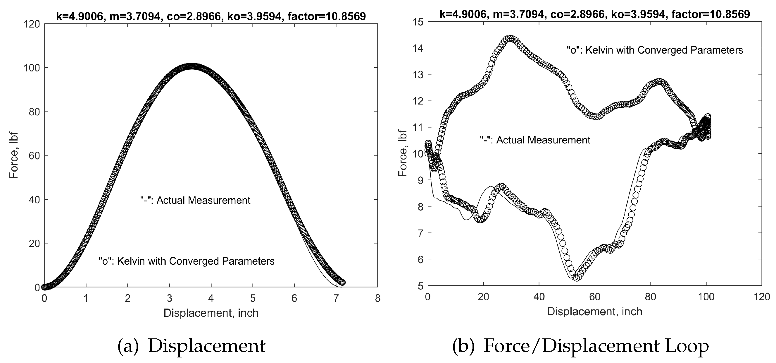
To validate the inverse optimization approach further and to test our hypothesis that the entire downhole sucker rod pump system can be approximated with the viscoelastic model, we employ the same procedures for another set of dynamometer measurements taken from the same V11 well at 7:14:19 am on August 7, 2019 Stroke 17, the exact load measurement recorded in TAM software examples, and obtain a different but similar set of system parameters with , , , and , and the scaling factor .
The convergence information is listed in Table 4. It is clear that the viscoelastic model does not match exactly with the sucker rod pump system. In addition, unlike the previous mathematical models from which the numerical or analytical solutions are derived, the data from the experiments are heuristic. Thus, the quadratic convergence properties of the Newton-Raphson iterative procedures are replaced with an oscillatory convergence with a rate much slower than the typical quadratic one observed for the Newton-Raphson iteration when the iterative solutions are within the neighborhood. Again, since the numerical evaluation of some of the Jacobian matrix entities has a truncation error around the converged system parameters will hover around that relative error range.
Again, the displacement and force/displacement loop match very well with the experimental data documented by Echometer Co as shown in Figure 5. Interestingly, the same system parameters have been applied to Stroke 18 and demonstrate a remarkable match with the actual experimental measurement.
Figure 6.
V11 well dynamometer measurement at 7:14:19 am on August 7, 2019 Stroke 17 and 18.
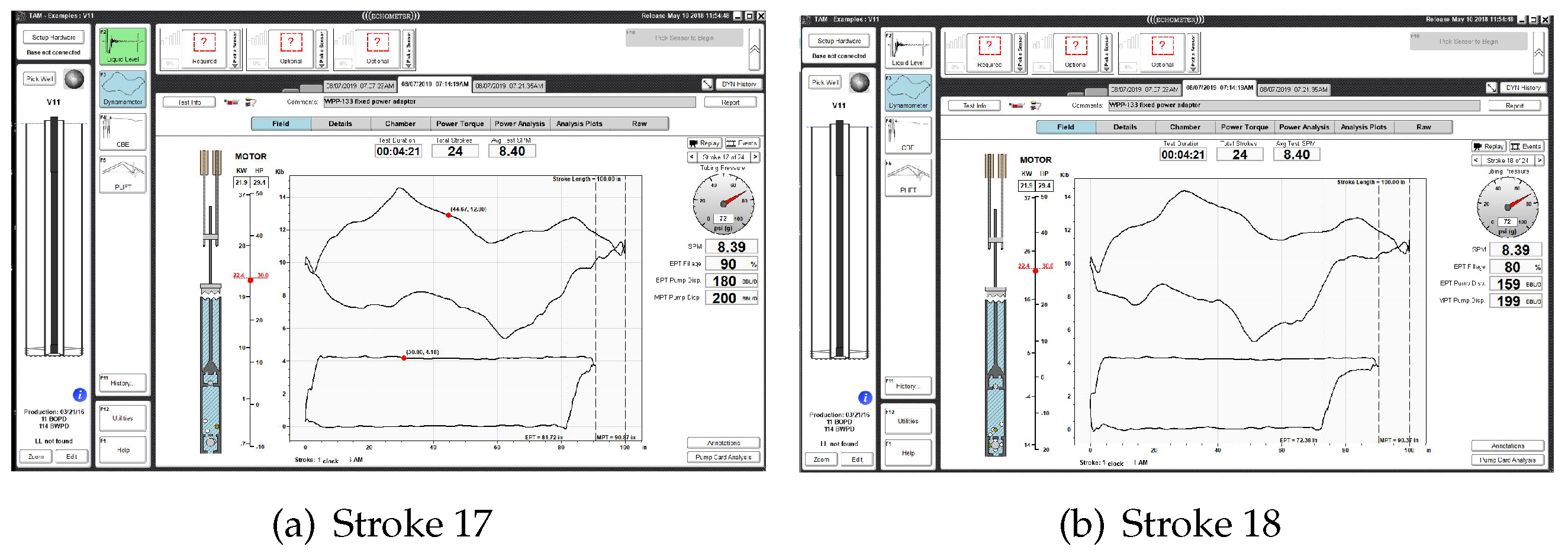
Figure 7.
Kelvin model analytical solutions with converged parameters in comparison with experimental measurements for Stroke 17.
Figure 7.
Kelvin model analytical solutions with converged parameters in comparison with experimental measurements for Stroke 17.
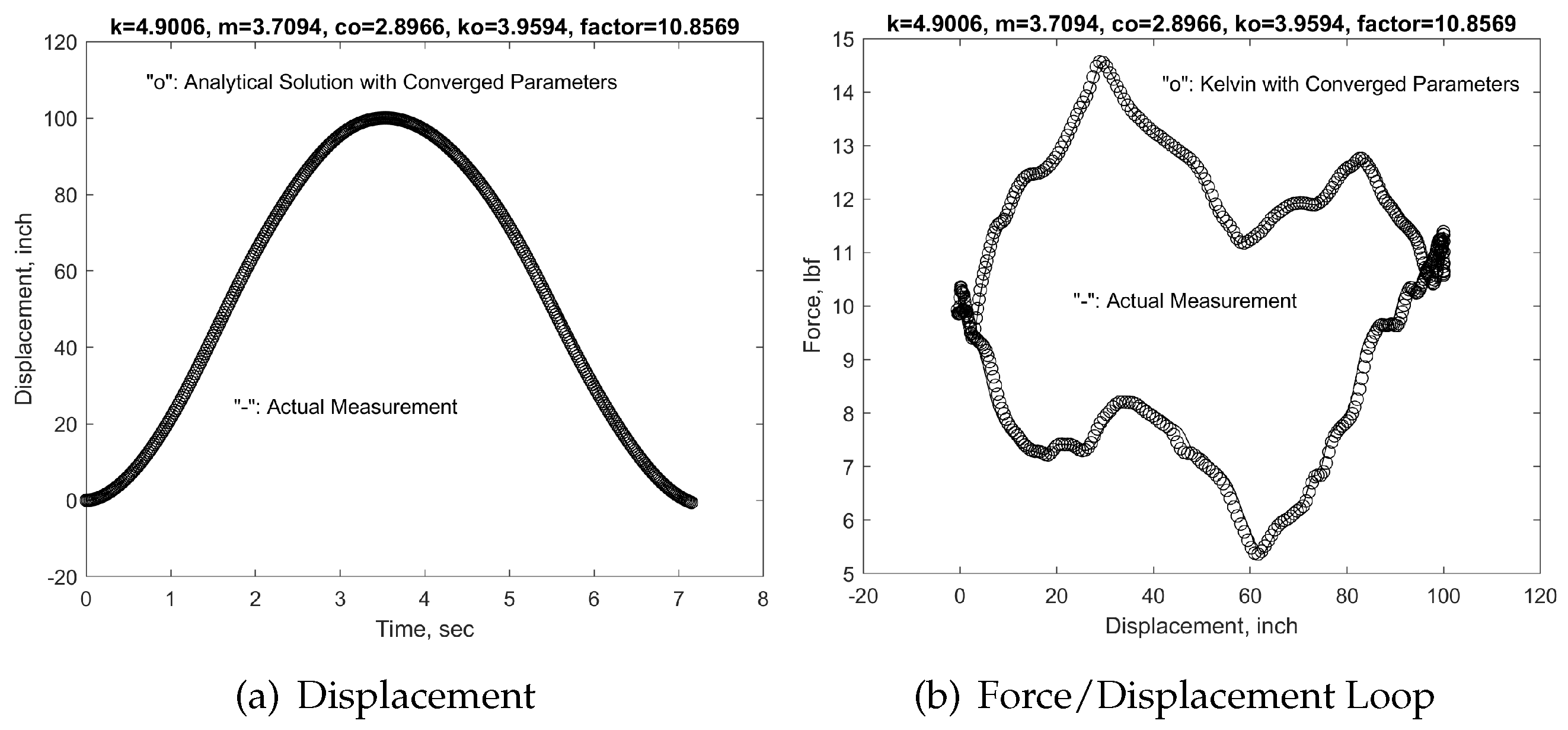
Figure 8.
Kelvin model analytical solutions with converged parameters in comparison with experimental measurements for Stroke 18.
Figure 8.
Kelvin model analytical solutions with converged parameters in comparison with experimental measurements for Stroke 18.
4. Conclusions
In the petroleum industry, it is very difficult to quantify the dynamical behaviors of the downhole sucker rod pump systems. The proposed inverse optimization method and the viscoelastic vibration model does shed light on the understanding of the reciprocal nature of the intricate relationship between the displacement of the polish rod and the total force exerted through the pump jack. The optimal parameters of the proposed viscoelastic model for the down-hole sucker rod pump system yield almost identical results in comparison with the experimental measurements in the oil filed. With this confirmation, the same approach will be implemented for the delivery system of a very viscous non-Newtonian fluid in EV manufacturing as well as other complex engineering systems. It is promising that even one- or two- parameters can be utilized to approximate complicated relationship between the required pressure drop and the flow rate with non-Newtonian internal fluid modeled with a power law distribution and bypass full-fledge computational models which normally require a lot of resources and experiences.
Author Contributions
Conceptualization, S.W. and D.G.; methodology, S.W.; software, S.W., D.G., A.W., K.B.; validation, S.W. and D.G.; formal analysis, S.W. and D.G.; investigation, S.W., D.G., A.W., K.B., S.E., C.T.; resources, S.W. and D.G.; data curation, S.W. and D.G.; writing—original draft preparation, S.W. and D.G.; writing—review and editing, S.W., D.G., A.W., K.B., S.E., C.T.; visualization, S.W.; supervision, S.W. and D.G.; project administration, S.W. and D.G.; funding acquisition, S.W. and D.G. All authors have read and agreed to the published version of the manuscript.
Funding
This research was partially supported by GM Research Grant.
Institutional Review Board Statement
Not applicable.
Informed Consent Statement
Not applicable.
Data Availability Statement
Not applicable.
Acknowledgments
The financial supports from the Midwestern State University, A Member of Texas Tech University System and Manufacturing Systems Research Lab, GM R&D are greatly appreciated
Conflicts of Interest
The authors declare no conflict of interest.
References
- Romero, O.J.; Almeida, P. Numerical simulation of the sucker-rod pumping system. Ing. Inv. 2014, 34, 4–11. [Google Scholar] [CrossRef]
- Karhan, M.K.; Nandi, S.; Jadhav, P.B. Design and optimization of sucker rod pump using prosper. International Journal of Interdisciplinary Research and Innovations 2015, 3, 108–122. [Google Scholar]
- Takacs, G. Improved designs reduce sucker-rod pumping costs. Oil & Gas Journal 1996, 94, 5. [Google Scholar]
- Yu, Y.; Chang, Z.; Qi, Y.; Xue, X.; Zhao, J. Study of a new hydraulic pumping unit based on the offshore platform. Energy Science & Engineering 2016, 4, 352–360. [Google Scholar]
- Anderson, G.; Liang, B.; Liang, B. The successful application of new technology of oil production in offshore. Foreign Oilfield Engineering 2001, 17, 28–30. [Google Scholar]
- Takacs, G. Modern sucker-rod pumping. In PennWell Books; Tulsa Oklahoma: location, 1993. [Google Scholar]
- Takacs, G. Sucker-rod pumping handbook - production engineering fundamentals and long-stroke rod pumping; Elsevier: location, 2015. [Google Scholar]
- Lea, J.F. What’s new in artificial lift?. World Oil, May 2012; pp. 79–85. Part I.
- Lea, J.F. What’s new in artificial lift?. World Oil, June 2012, pp. 85–94. Part II.
- Bommer, P.M.; Podio, A.L. The Beam Lift Handbook; PETEX: location, 2012. [Google Scholar]
- Podio, A. Artificial lift. Encyclopedia of Life Support Systems 2013, 1–9. [Google Scholar]
- Takacs, G. Sucker rod pumping manual; PennWell Corporation: Tulsa, 2003. [Google Scholar]
- Dong, Z.; Zhang, M.; Zhang, X.; Pang, X. Study on reasonable choice of electric submersible pump. Acta Petrolei Sinica 2008, 29, 128–131. [Google Scholar]
- Karpuz-Pickell, P.; Roderick, R. From failure to success: A metallurgical story on sucker rod pump barrels. In Proceeding of the Sixty Second Annual Meeting of the Southwestern Petroleum Short Course. Lubbock, Texas, 22–23 April 2015. [Google Scholar]
- Nampoothiri, M.P. Evaluation of the effectiveness of api-modified goodman diagram in sucker rod fatigue analysis. Texas Tech MS Thesis, 2001. [Google Scholar]
- Wang, S.; Yang, Y.; Wu, T. Model studies of fluid-structure interaction problems. Computer Modeling in Engineering and Sciences 2019, 119, 5–34. [Google Scholar] [CrossRef]
- Wang, S.; Grejtak, T.; Moody, L. Structural designs with considerations of both material and structural failure. ASCE Practice Periodical on Structural Design and Construction 2017, 22, 1–8. [Google Scholar] [CrossRef]
- Li, Z.; Song, J.; Huang, Y. . Design and analysis for a new energy-saving hydraulic pumping unit. Proc IMechE, Part C: Journal of Mechanical Engineering Science, 2017. [Google Scholar]
- Rowlan, O.L.; McCoy, J.N.; Lea, J.F. Use of the pump slippage equation to design pump clearances. Private Communication, 2012. [Google Scholar]
- Nouri, J.M.; Whitelaw, J.H. . Flow of newtonian and non-newtonian fluids in a concentric annulus with rotation of the inner cylinder. ASME Journal of Fluids Engineering 1994, 116, 821–827. [Google Scholar] [CrossRef]
- Fakher, S.; Khlaifat, A.; Hossain, M.; Nameer, H. A comprehensive review of sucker rod pumps’ components, diagnostics, mathematical models, and common failures and mitigations. J. Pet. Explor. Prod. Technol. 2021, 11, 3815–3839. [Google Scholar] [CrossRef]
- Patterson, J.; Chambliss, K.; Rowlan, L.; Curfew, J. Fluid slippage in down-hole rod-drawn oil well pumps. Proceedings of the 54th Southwestern Petroleum Short Course 2007, 11, 45–59. [Google Scholar] [CrossRef]
- Patterson, J.; Williams, B. . Fluid slippage in down-hole rod-drawn oil well pumps. Proceedings of the 45th Southwestern Petroleum Short Course 1998, 11, 180–191. [Google Scholar]
- Zhao, R.; Zhang, X.; Liu, M.; Shi, J.; Su, L.; Shan, H.; Sun, C.; Miao, G.; Wang, Y.; Shi, L.; Zhang, M. Production optimization and application of combined artificial-lift systems in deep oil wells. SPE Middle East Artificial Lift Conference(1-10), November. 2016, SPE-184222-MS.
- Patterson, J.; Dittman, J.; Curfew, J.; Hill, J.; Brauten, D.; Williams, B. Fluid slippage in down-hole rod-drawn oil well pumps. Proceedings of the 46th Southwestern Petroleum Short Course 1999, 11, 96–106. [Google Scholar]
- Patterson, J.; Curfew, J.; Brock, M.; Brauten, D.; Williams, B. . Fluid slippage in down-hole rod-drawn oil well pumps. Proceedings of the 47th Southwestern Petroleum Short Course 2000, 11, 117–136. [Google Scholar]
- Pons, V. Modified everitt-jennings: A complete methodology for production optimization of sucker rod pumped wells. Proceeding of the Sixty Second Annual Meeting of the Southwestern Petroleum Short Course, Lubbock, Texas, 22–23 April 2015. [Google Scholar]
- Wang, S.; Rowlan, L.; Henderson, A.; Aleman, S.T.; Creacy, T.; Taylor, C.A. Viscoelastic representation of the operation of sucker rod pumps. Fluids 2021, 7, 1–12. [Google Scholar] [CrossRef]
- Bommer, P.M.; Podio, A.L.; Carroll, G. . The measurment of down stroke force in rod pumps. Proceeding of the Sixty Third Annual Meeting of the Southwestern Petroleum Short Course, Lubbock, Texas, 20–21 April 2016. [Google Scholar]
- Wang, S. Scaling, complexity, and design aspects in computational fluid dynamics. Fluids 2021, 6, 1–17. [Google Scholar] [CrossRef]
- Wang, S.; Rowlan, L.; Cook, D.; Conrady, C.; King, R.; Taylor, C. Dynamics of pump jacks with theories and experiments. Upstream Oil and Gas Technology 2023, 11, 1–7. [Google Scholar] [CrossRef]
- Wang, S.; Rowlan, L.; Elsharafi, M.; Ermila, M.; Grejtak, T.; Taylor, C. On leakage issues of sucker rod pumping systems. ASME Journal of Fluids Engineering 2019, 141, 111201–111207. [Google Scholar] [CrossRef]
- Copeland, C. Fluid extractor. Proceeding of the Sixty Second Annual Meeting of the Southwestern Petroleum Short Course, Lubbock, Texas, 22–23 April 2015. [Google Scholar]
- Ermila, M. Critical evaluation of sucker-rod string design practices in the hamada field libya. University of Miskolc MS Thesis, 1999. [Google Scholar]
- Wang, S. Essentials of Mathematical Tools for Engineers; Sentia Publishing: location, 2022. [Google Scholar]
- Wang, S. Fundamentals of Fluid-Solid Interactions-Analytical and Computational Approaches; Elsevier Science: location, 2008. [Google Scholar]
- Bathe, K. Finite Element Procedures; Prentice Hall: location, 1996. [Google Scholar]
Figure 1.
Typical viscoelastic models.
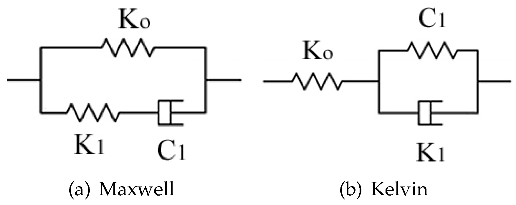
Figure 2.
Typical responses for Maxwell and Kelvin models.
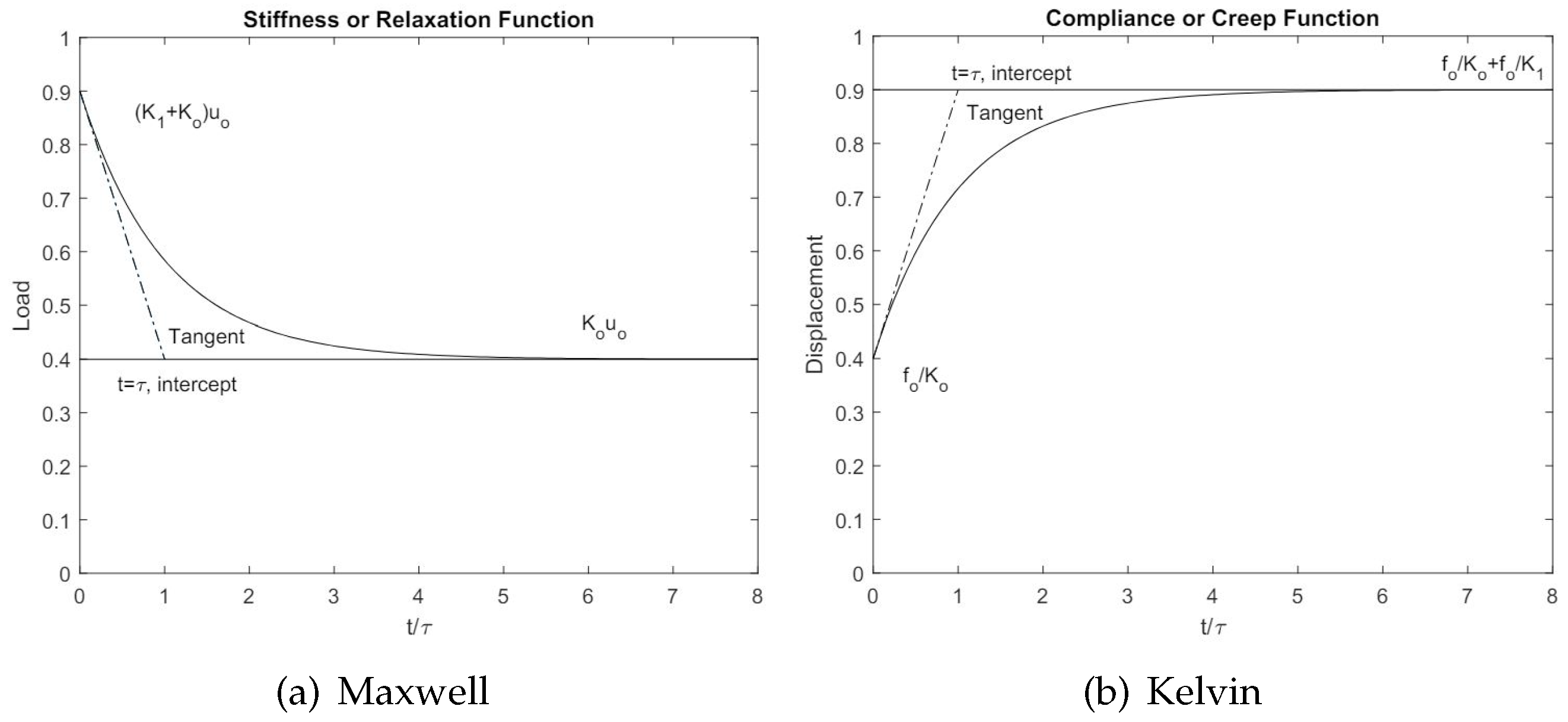
Figure 3.
Kelvin viscoelastic vibration system response.
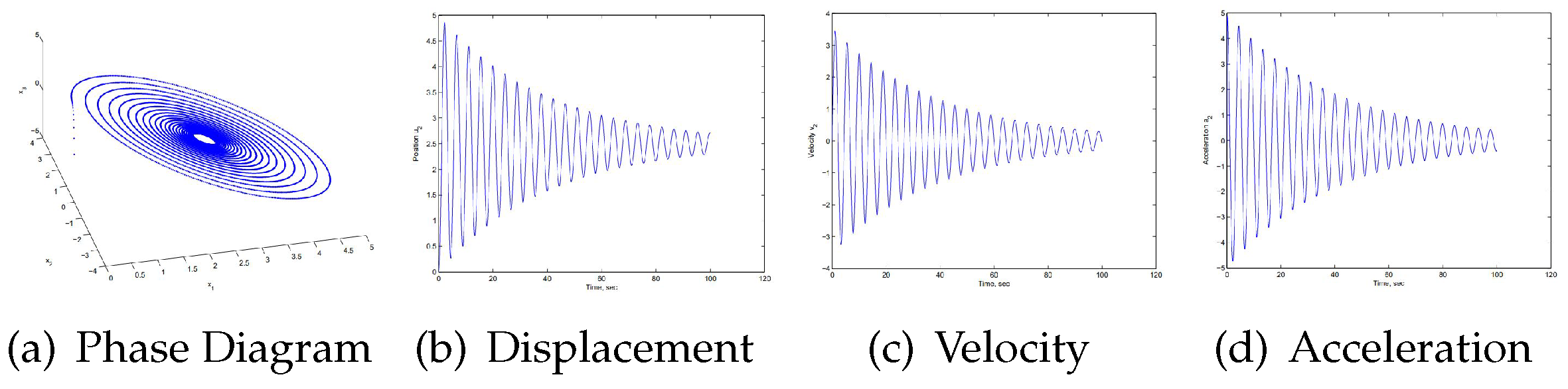
Figure 4.
Maxwell viscoelastic vibration system response.
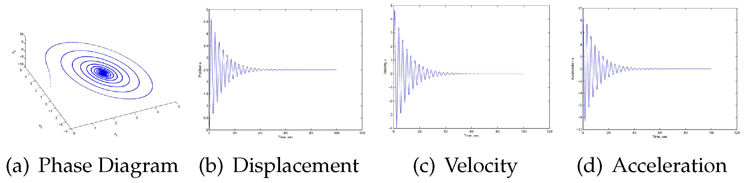
Figure 5.
A Kelvin viscoelastic vibration system with the converged parameters.
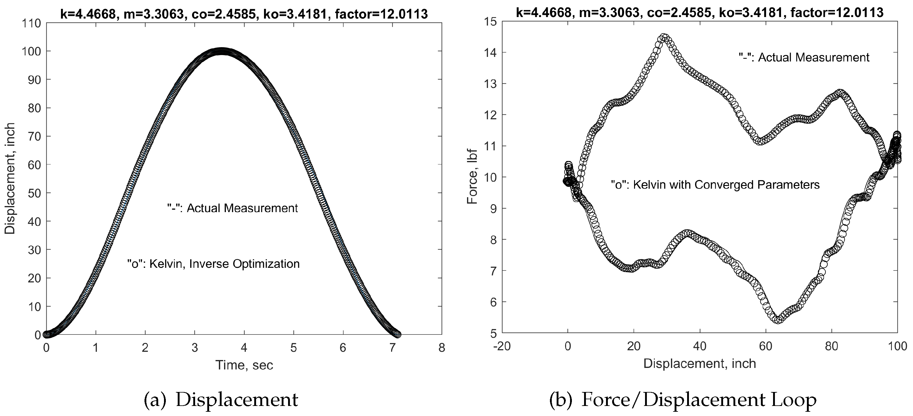

Table 1.
Newton-Raphson iteration convergence of the relaxation time , the scaling factor C, and the relative incremental error as defined in Eq. (16) with the logarithmic modification.
Table 1.
Newton-Raphson iteration convergence of the relaxation time , the scaling factor C, and the relative incremental error as defined in Eq. (16) with the logarithmic modification.
| No. | C | ||
|---|---|---|---|
| 24 | 4.113353577899 | 1.108643414669 | 0.8481099309715 |
| 25 | 4.808147443754 | 1.012180228335 | 0.3507291199584 |
| 26 | 4.991132754710 | 1.001324920436 | 0.0916535074825 |
| 27 | 5.004938782496 | 1.000004471816 | 0.0069345149036 |
| 28 | 5.005001665203 | 1.000000000128 | 0.0000315207506 |
| 29 | 5.005001666667 | 1.000000000000 | 0.0000000007343 |
Table 2.
Newton-Raphson iteration convergence of the relaxation time , the scaling factor D, and the relative incremental error as defined in Eq. (16) with the logarithmic modification.
Table 2.
Newton-Raphson iteration convergence of the relaxation time , the scaling factor D, and the relative incremental error as defined in Eq. (16) with the logarithmic modification.
| No. | D | ||
|---|---|---|---|
| 7 | 5.3502492856171 | 0.1709734105086 | 0.3327036938013 |
| 8 | 5.7906235191341 | 0.0500242875435 | 0.2283408394767 |
| 9 | 5.9764971771645 | 0.0062271928244 | 0.0954819384169 |
| 10 | 6.0044277938157 | 0.0001228805887 | 0.0142949464357 |
| 11 | 6.0050011491776 | 0.0000000513466 | 0.0002931822785 |
| 12 | 6.0050013888888 | 0.0000000000000 | 0.0000001225744 |
Table 3.
Newton-Raphson iteration convergence of the system parameters m, c, and k, the scaling factor C, and the relative incremental error as defined in Eq. (16).
Table 3.
Newton-Raphson iteration convergence of the system parameters m, c, and k, the scaling factor C, and the relative incremental error as defined in Eq. (16).
| No. | m | c | k | C | |
|---|---|---|---|---|---|
| 2 | 14.0088697014 | 38.8505562741 | 252.2630700 | 4.4695001143 | 7.5404751904 |
| 3 | 9.8962841404 | 14.3998130515 | 260.9769377 | 1.4358822096 | 0.8809455612 |
| 4 | 9.8402652289 | 7.0242940976 | 247.2775516 | 1.0914951778 | 0.5182224546 |
| 5 | 9.8739033983 | 5.2106554463 | 247.1593685 | 1.0123649473 | 0.0605886943 |
| 6 | 9.8798105710 | 4.9450642071 | 246.9998836 | 1.0002193760 | 0.0103258241 |
| 7 | 9.8799373442 | 4.9399706629 | 246.9979158 | 1.0000000949 | 0.0001820245 |
| 8 | 9.8799373906 | 4.9399686098 | 246.9979147 | 1.0000000016 | 0.0000000768 |
Table 4.
Newton-Raphson iteration convergence of the system parameters k, m, , and , the scaling factor C, and the relative incremental error as defined in Eq. (16).
Table 4.
Newton-Raphson iteration convergence of the system parameters k, m, , and , the scaling factor C, and the relative incremental error as defined in Eq. (16).
| No. | k | m | C | |||
|---|---|---|---|---|---|---|
| 10 | 4.8145200 | 3.7227113 | 3.0371959 | 4.0113022 | 9.9459747 | 0.0583832 |
| 11 | 4.8157944 | 3.7250974 | 3.0323557 | 4.0186058 | 9.9727830 | 0.0336033 |
| 12 | 4.8769304 | 3.71661320 | 2.9368406 | 3.9800812 | 10.5630007 | 0.0518076 |
| 13 | 4.8762824 | 3.7159651 | 2.9388687 | 3.9795838 | 10.5762036 | 0.0011525 |
| 14 | 4.8948972 | 3.7115266 | 2.9074872 | 3.9649666 | 10.7825937 | 0.0180758 |
| 15 | 4.8951385 | 3.7107580 | 2.9057328 | 3.9636912 | 10.7948712 | 0.0010746 |
| 16 | 4.8989279 | 3.7098281 | 2.8993963 | 3.9606940 | 10.8378530 | 0.0037609 |
| 17 | 4.8999700 | 3.7095979 | 2.8977176 | 3.9599161 | 10.8495151 | 0.0010198 |
| 18 | 4.9004231 | 3.7094863 | 2.8969610 | 3.9595585 | 10.8546888 | 0.0004526 |
| 19 | 4.9005655 | 3.7094541 | 2.8967290 | 3.9594508 | 10.8562851 | 0.0001396 |
| 20 | 4.9006119 | 3.7094470 | 2.8966611 | 3.9594212 | 10.8567655 | 0.0000420 |
| 21 | 4.9006292 | 3.7094476 | 2.8966428 | 3.9594152 | 10.8569094 | 0.0000126 |
Disclaimer/Publisher’s Note: The statements, opinions and data contained in all publications are solely those of the individual author(s) and contributor(s) and not of MDPI and/or the editor(s). MDPI and/or the editor(s) disclaim responsibility for any injury to people or property resulting from any ideas, methods, instructions or products referred to in the content. |
© 2024 by the authors. Licensee MDPI, Basel, Switzerland. This article is an open access article distributed under the terms and conditions of the Creative Commons Attribution (CC BY) license (http://creativecommons.org/licenses/by/4.0/).
Copyright: This open access article is published under a Creative Commons CC BY 4.0 license, which permit the free download, distribution, and reuse, provided that the author and preprint are cited in any reuse.


