
Submitted:
11 April 2024
Posted:
15 April 2024
You are already at the latest version
Abstract
In Indonesia, types of meat are still identified manually due to increasing prices for beef and buf-falo ahead of Idul Fitri. Traders mix beef with pork to thwart the beef scam. Haar wavelet and GLCM, GLCM with angles of 0°, 45°, 90°, and 135°, as well as matrices using contrast, correlation, energy, homogeneity, and entropy, are used in feature extraction. The following are the results of meat image classification testing using k-NN, Haar wavelet, and GLCM: The k-NN algorithm shows superiority in identifying fresh (99%), frozen (99%), and rotten (96%) meat texture images with the most fantastic accuracy results in every situation. Meanwhile, GLCM routinely provides good results, especially regarding the texture image of fresh meat (183.21) and rotten meat (115.79). However, despite delivering less throughput than k-NN and GLCM, Haar wavelets are still helpful, especially when dealing with fresh meat texture images (89,96).
Keywords:
meat type texture image classification
; image processing
; wavelet haar
; Gray level Cooccurrence Matrix (GLCM)
; K-Nearst Neighbor (K-NN)
1. Introduction
One food that is high in animal protein is meat. Indonesia's population and the country's need for meat is growing. Many traders purposefully combine pig and beef to earn significantly [1]. Beef sales in Indonesia are declining ahead of Eid al-Fitr due to rising beef prices. In anticipation of this, some traders blend pork and beef. The pork was used because it was less expensive and had a comparable colour and texture to meat. It's challenging for the average person to distinguish between beef and pig with unaided eyes [2]. The Indonesian National Standards Agency (2018) states that the colour, texture, tenderness, and marbling of the fat and meat are the primary factors used to evaluate the physical quality of beef [3]. For the development of human resources, public nutrition is crucial in Indonesia, and beef is one type of animal protein. Bright red, shiny but not pallid, elastic but not sticky, and with a distinct aroma are all signs of healthy meat [4]. The quality of beef is determined by various factors such as the flesh's size, texture, colour, and aroma. These days, meat quality is determined by its colour and shape. Nevertheless, this method still has certain shortcomings because of subjectivity and human judgment, which aren't always reliable [5].
Since food authenticity is a trendy topic, food fraud is a global issue that has drawn attention in recent decades. The most popular meats, significant for culture and religion, economics, and nutrition, are beef, buffalo, chicken, duck, goat, sheep, and pork. Both their raw and processed forms are frequently discovered to be contaminated [6]. Concerns against meat are numerous, ranging from religious to legal to economic to medical. To shield customers from deceit and poor marketing practices, several analytical approaches have been proposed to identify meat species separately or in combined samples [7]. Meat product species substitution is a prevalent issue that has been documented globally. Using low-value meat resources to create high-value meat products is known as food fraud, and it is typically done to profit financially. Financial, health, and religious issues are among the repercussions [8].
Adulteration of meat, primarily for commercial gain, is pervasive and poses significant threats to public health as well as moral and religious offences. Technology for fast, precise, and dependable detection is essential for efficiently tracking meat adulteration. Given the significance and quick development of meat adulteration detection technology, it would be beneficial to thoroughly analyse recent developments in this area and recommend future paths for advancement [9]. Cattle, buffalo, and pigs are familiar sources of tainted ingredients, so their calculations may preserve social, religious, economic, and health purity [10]. Choosing an adequate image texture quality is one of the primary issues with texture classification [11]. To ascertain if raw meat texture traits are a reliable indicator of tenderness in beef [12]. A technique for differentiating between turkey and pig ham grades was created by utilizing wavelet texture and colour characteristics [13]. These researchers used practical procedures to evaluate various texture analysis techniques and regression methods to predict multiple physico-chemical and sensory attributes of distinct cuts of Iberian pork. Statistical methods like Haralick descriptors, local binary patterns, fractal features, and frequency descriptors like Gabor or wavelet features are examples of texture descriptors [14]. Experiments evaluating pork quality indicate that the two-dimensional Gabor wavelet transform is a more effective method for extracting the textural properties of pork [15].
This study suggests using long short-term memory (DWTLSTM) with a discrete wavelet transform to mitigate noise contamination of e-nose signals during beef quality monitoring. Our approach performs well, with an average accuracy of 94.83% and an average F-measure of 85.05% in classifying beef quality [16]. The technique is based on clustering, and Haar filters are used carefully to extract features in the wavelet transform domain. First, second, and third-level decomposition in the wavelet domain was performed, and the coefficients produced at each level were examined to forecast the freshness of fish samples [17]. Sheep muscle classification was achieved using wavelet analysis of near-infrared (NIR) hyperspectral imaging data. To determine the optimal wavelet features for classifying sheep muscles, apply wavelet transform [18].
To get 64-dimensional characteristics of excellent quality, eight picture texture features are extracted under each of the final eight wavelengths using a two-dimensional Gabor wavelet transform [15]. A half-pig carcass can be accurately depicted by utilizing the capabilities of wavelet spectral graphics, referred to as SpectralWeight. Next, SpectralWeight was applied as a prediction model to weigh different pieces of pork and determine the tissue composition [19]. Discrete Wavelet Transform and Long Short-Term Memory (DWTLSTM) are suggested to be used in conjunction with interference to prevent e-nose signal contamination for evaluating beef quality [20]. To forecast TVB-N values in cooked beef during storage, this study examines the integration of spectral and image data from visible and near-infrared hyperspectral imaging. Nine ideal wavelengths were chosen using the sequential projection algorithm (SPA) and variable no elimination (UVE). Discrete wavelet transform (DCT) extracted 36 single values as texture features [21].
This study uses picture preprocessing, data set training, and classification to assess the quality of tuna flesh classes according to colour space. Cropping, converting RGB images to HSV, and employing wavelets to extract features are the three main steps in the preprocessing of images. The findings demonstrate that Symlet wavelets yield a higher correlation coefficient between feature extraction levels than Haar wavelets. Wavelet Symlet and k-NN classify 65 test picture datasets with a higher accuracy of 81.8% than wavelet Haar k-NN's 80.3% [22]. The amount of intramuscular fat (IMFAT) in beef ribeye muscle has been predicted using multiresolution texture analysis techniques utilizing wavelet transformation. Several features are computed from the 2-D wavelet decomposed ultrasound image using the Haar wavelet as a basis function to create a fast wavelet transform [23]. A new technique for local thresholding that uses weighted detail coefficients in wavelet synthesis to generate a multiscale thresholding function for picture segmentation. The fast wavelet technique can implement this local wavelet-based threshold method, which adjusts to the local environment and size. We used X-ray imaging to apply this method to detect physical contamination in chicken inspections [24].
The features are carefully extracted using Haar filters in a domain wavelet transform. First, second, and third-level decomposition in the wavelet domain was performed, and the coefficients produced at each level were examined to forecast the freshness of fish samples [25]. The amount and percentage of intra-muscular fat (IMFAT) is the primary element in determining beef quality. Texture analysis was used on B-mode ultrasound pictures of live beef calf muscle ribeyes to predict their IMFAT. We apply the gray-level co-occurrence matrix (GLCM) method to multiresolution analysis of textures and second-order statistics using wavelet transform (WT) [26]. The purpose of this study is to use digital photographs to distinguish the distinctions between beef and pork. For texture analysis, colour features use the Gray Level Co-Occurrence Matrix to calculate a first-order statistical average of colour values [27]. A technique has been created to extract the texture of beef, which is a crucial component in the classification of beef. Utilizing Discrete Wavelet Transform (DWT) frequency domain and Gray Level Co-occurrence Matrix (GLCM) statistics, texture feature analysis extraction is performed [28].
This study aims to determine the freshness levels of chickens by analyzing their colour and texture. The gray-level co-occurrence matrix (GLCM) is the texture property utilized [29]. We incorporate and apply its contrast, energy, and homogeneity properties into CNN learning for GLCM's capacity to identify patterns with significant variances, robustness to geometric distortion, and straightforward transformation [30]. This study aimed to categorize and distinguish between sizable groups of distinct cattle accurately. The gray level co-occurrence matrix (GLCM) was employed to extract picture features [31]. In this study, we used the Support Vector Machines classifier to create a system that can identify beef quality based on its colour and texture characteristics. Statistical techniques and the Gray Level Co-Occurrence Matrix (GLCM) method are employed for feature extraction [32]. This study aims to identify the grade of beef that is fit for human consumption. The K-NN algorithm is used to categorize photos of meat using the co-occurrence matrix. Based on colour and texture, this research can be utilized to distinguish between different varieties of meat [33]. To extract texture properties (contrast, correlation, energy, and homogeneity), the grey-level co-occurrence matrix (GLCM) was used for the hyperspectral image's first-principle component image, which had a 98.13% variance [34].
This study aims to evaluate the precision of tilapia fish computations made with the K-Nearest Neighbor (K-NN) algorithm and digital image processing techniques. Customers can use a smartphone as a visualization to determine whether the fish is fit for ingestion [35]. This study attempts to assess the freshness of fish using fish-eye image-based Naïve Bayes (NB) and k-nearest neighbour (K-NN) classification techniques. These findings indicate that the K-NN approach outperforms NB, with average values for accuracy, precision, recall, specificity, and AUC of 0.97, 0.97, 0.97, 0.97, and 0.97 [36]. A mutton image classification model is created using several practical modelling algorithms, such as k-nearest neighbour (KNN), to determine the authenticity of fresh and cooked food. Kebab is made of mutton [37].
The suggested approach uses preprocessed meat marbling picture segments with contrast enhancement and illumination normalization. The fat pixels are described intramuscularly, and attribute scores are determined by the learning step's definition of the required meat standards. The learning method is an instance-based system that assigns scores to segmentation outcomes using the k-Nearest Neighbors (k-NN) algorithm [38]. This study not only identifies the kind of meat but also, for the first time, distinguishes between distinct body parts and meat. The outcomes of the suggested approach are juxtaposed with other machine learning algorithms employed in prior investigations, including k-nearest neighbours (k-NN) and fundamental deep learning [39]. Pork sausages were classified using linear and non-linear techniques, including k-nearest neighbours (k-NN), to distinguish between them [40]. This paper provides an innovative and reliable biometrics-based method for identifying cow tails. Two additional classifiers, Fuzzy-k-Nearest Neighbor (Fk-NN) and K-Nearest Neighbor (k-NN), were utilized to validate the findings produced by this classifier [41]. By gathering and evaluating olfactory data, the electronic nose—a non-destructive detection method—can determine the freshness of meat. In contrast to traditional machine learning techniques like K Nearest Neighbors (KNN), pre-drilled AlexNet, GoogLeNet, and ResNet models are re-drilled in the last three layers [42].
This study examined how well the MicroNIR device (VIAVI, Santa Rosa, CA) could use distance to K-Nearest Neighbor (K-NN) cluster analysis and multivariate data analysis to coordinate the fermentation process of dry sausage [43]. With 97.4% accuracy, the k-nearest neighbour (KNN) model learns and categorizes the features of ApSnet segmented images [44]. The first derivative spectrum is used in K-nearest-neighbors (KNN) classification [45]. The new cattle recognition system uses hybrid textures and muzzle point pattern features to identify and categorise cow breeds. K-nearest neighbour (K-NN) and other classification models are used in the classification of cows [46]. The k-nearest neighbour technique is used to construct the model [47].
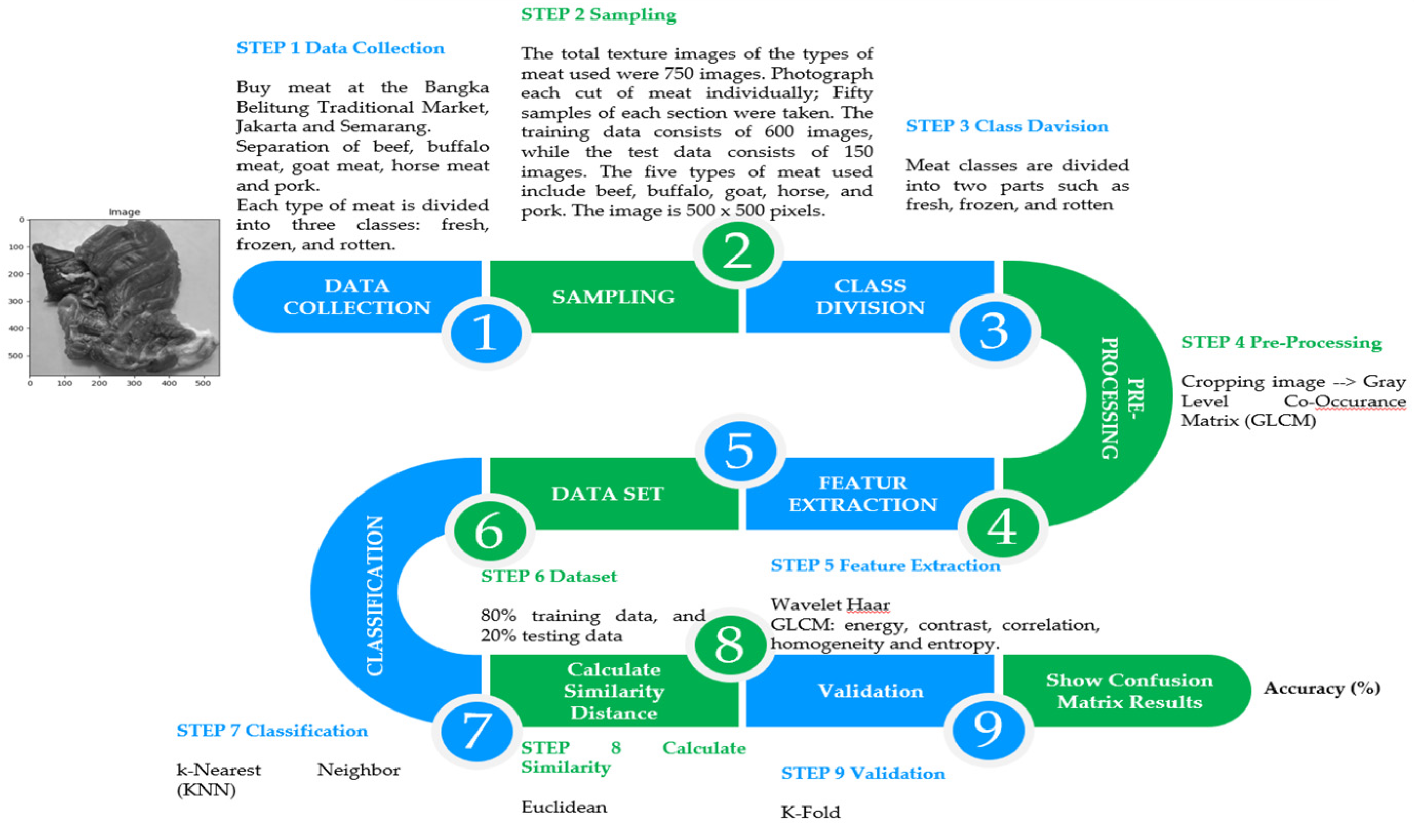
Figure 1.
Steps in the process of classifying meat texture images.
2. Materials and Methods
2.1. Data Retrieval
This study used five different kinds of meat: bacon, buffalo, goat, horse, and cattle. The meat is cut around 15 × 15 cm into pieces by slicing it lengthwise or against the grain. Three categories exist for one sort of meat: fresh beef, frozen beef, and rotten beef. We collected as many as fifty pieces of fresh meat, fifty pieces of frozen beef, and fifty pieces of decaying beef with each sample. Thus, 150 pieces of fresh, frozen, and rotten meat samples were taken. One hundred fifty pieces times five different types of beef are 750 samples if five different varieties of meat are used. Texture photographs of the various meat types were captured using a digital camera. Perpendicular image acquisition was accomplished by adjusting the image-taking distance. The distances to take pictures were 10, 20, 30, and 40 cm. Here, the room illumination is provided by illumination Emitting Diode (LED) bulbs, which come in wattages of 3, 5, 7, 9, 11, and 13 respectively.
2.2. Pre-Processing
Texture image features of meat types are obtained using an image feature extraction approach. There are several pre-processing steps in image processing before features are extracted. GLCM is a feature used to extract images of meat texture. The purpose of image cropping is to remove labels on images that have a texture similar to meat. Texture image features of meat types are obtained using an image feature extraction approach. There are several pre-processing steps in image processing before features are extracted. GLCM is a feature used to extract images of meat texture. The purpose of image cropping is to remove labels on images that have a texture similar to meat.
2.3. Feature Extraction
The final stage of image processing is extracting image characteristics as attributes of the classification process. The GLCM (Gray Level Co-occurrence Matrices) and Wavelet Haar features are two examples of this feature. Five features are included in the histogram feature: energy, contrast, homogeneity, correlation, and entropy. Meanwhile, energy, contrast, correlation, homogeneity and entropy are the five GLCM properties used in this research.
2.4. Meat Sample Collection
Extracting image properties as attributes for the classification process is the final step in the image processing process. Two examples of these features are the Wavelet Haar feature and GLCM (Gray Level Co-occurrence Matrices). The histogram feature consists of the following five features: entropy, energy, contrast, homogeneity, and correlation. Meanwhile, the five GLCM qualities used in this research are energy, contrast, correlation, homogeneity and entropy.
2.5. Sampling
Seven hundred fifty images show various types of meat textures. Take separate pictures of each cut of meat. Each type of beef has been tried fifty times. Are 600 photos in the training set and 150 in the test set? Beef, buffalo, goat, horse and pork are the five types of meat used. Images were taken at a resolution of 500×500 pixels.
2.6. k-Nearest Neighbor (k-NN)
The results indicate that the k-nearest neighbour algorithm has the highest accuracy among algorithms for categorizing and comparing k-nearest neighbour patterns based on accuracy [48]. The k-nearest neighbours (k-NN) method is employed to process data [49]. In classification tasks, the class majority of K's nearest neighbours are used by k-NN to derive the class label of an input data point. When utilizing the k-NN approach for classification, the new data's class is determined by comparing it to most of the K nearest neighbours' courses in the training dataset. The K-Nearest Neighbour approach is used to classify things using learning data near the object and the number of nearest neighbours, or the k value. Using the Euclidian distance method, the following formula is typically used to determine a neighbour's proximity or distance.
With:
| : euclidien distance between vector x and y | |
| : distance testing data to training data | |
| : testing data -j, with j = 1,2,..., n | |
| : training data -j, with j = 1,2,...., n | |
| : amount of feature. |
The distance between each data point in the training dataset and the data point to be predicted is measured as part of the k-NN computation. The following are the primary steps in k-NN calculations:
- The distance metric used to calculate the proximity between data points should be chosen. Euclidean distance is the distance metric that is employed.
- Using the Euclidean distance metric, determine the distance to each data point in the training dataset and the distance for each test data point.
- After computing the distance, find the k-nearest neighbours; see the test data points' k-nearest neighbours based on the most negligible distance value. Sorting the calculated distances and choosing the lowest K value will do this.
- Predicting a class (classification) As the class prediction for the test data point, if the task involves classification, ascertain the majority class of the k-nearest neighbours.
Figure 2.
Classification of texture images of meat types using the k-Nearest Neighbor (k-NN) approach.
Figure 2.
Classification of texture images of meat types using the k-Nearest Neighbor (k-NN) approach.
2.6.1. Performance Evaluation of Classification Results
The confusion matrix is a valuable tool for assessing classification models' performance in predicting the proper class. The confusion matrix consists of four primary components: False Positive (FP), True Negative (TN), True Positive (TP), and False Negative (FN). As a result of classifying texture photos of several meat varieties, Table 1 displays the classification performance in Confusion matrix form. There are four options based on Table 1 of the confusion matrix: a true positive (TP) is an instance that is positive and classed as positive; a false negative (FN) is an instance that is grouped as unfavourable. A true negative (TN) is an instance that has been declared hostile; a false positive (FP) is an instance that has been declared positive.True Positive (TP): The number of positive observations correctly predicted by the model.
- True Negative (TN): The number of negative observations correctly predicted by the model.
- False Positive (FP): The number of negative observations incorrectly predicted as positive by the model (Type I error).
- False Negative (FN): The number of positive observations incorrectly predicted as negative by the model (Type II error).
2.6.2. Validation
The possibility that a picture is considered to be of good quality and that the image is indeed of good quality is known as sensitivity. Equation 2 can be used to compute sensitivity.
Specificity is the likelihood that a picture is perceived as being of low quality and actually of low quality. Equation 3 is used to calculate specificity.
By dividing the number of classifications by the number of correct classifications, as shown in Equation 4, one can describe the accuracy of the classification success.
2.7. Wavelet Haar
The Discrete Wavelet Transform (DWT), which is based on the Haar wavelet basis function, was used to reduce the dimensionality of the data. The algorithm coefficients and prediction time consumption are better with DWT (wavelet basis function and number of transformation layers are Haar-4, respectively) [50]. One kind of wavelet function utilized in wavelet analysis is the Haar wavelet. The wavelet function is a mathematical tool for simultaneously analyzing and representing texture images of different meat types or data in the time and frequency domains. The Dutch mathematician Alfréd Haar, who first presented this function in 1910, is honoured with the Haar wavelet.
The Haar wavelet is one of the simplest wavelets to comprehend and use because of its discrete and straightforward character. The Haar wavelet function is a local segment function frequently used in data compression, image processing, and image analysis because it can quickly identify variations in texture photographs of different types of meat. The image is separated into smaller intervals for the Haar wavelet transform, and each interval is then subjected to the Haar wavelet. This procedure enables depicting pictures on distinct signal components at varying resolutions. Since Haar wavelets' primary benefit is their ability to deliver high-frequency information effectively, they are frequently employed in applications where quickly identifying edges or changes in the signal is crucial. An approximation coefficient and details-based mathematical formula can be used to explain the Haar wavelet transform. For a discrete signal with length approximation coefficient and detail coefficients at level k can be calculated as follows:
- Approximation Coefficient:
- Detailed Coefficients:
This process can be repeated at each transformation level by replacing with for the next level. Basic steps to perform the Haar wavelet transform:
- Intervals for texture photos of different kinds of meat are divided into smaller intervals. A convolution operation on neighbouring intervals or the average of two successive values can accomplish this.
- Once the intervals have been separated, compute the approximation coefficient (A) and the detail coefficient (D). The ap-proximation coefficient represents the finer details or low-frequency components in a meat type's texture image. Detail coefficients represent high-frequency elements or information that is coarser or changes more quickly.
- Normalize the coefficient values to suit the requirements of a particular use case. Scale adjustments or weight assignments could be part of this process.
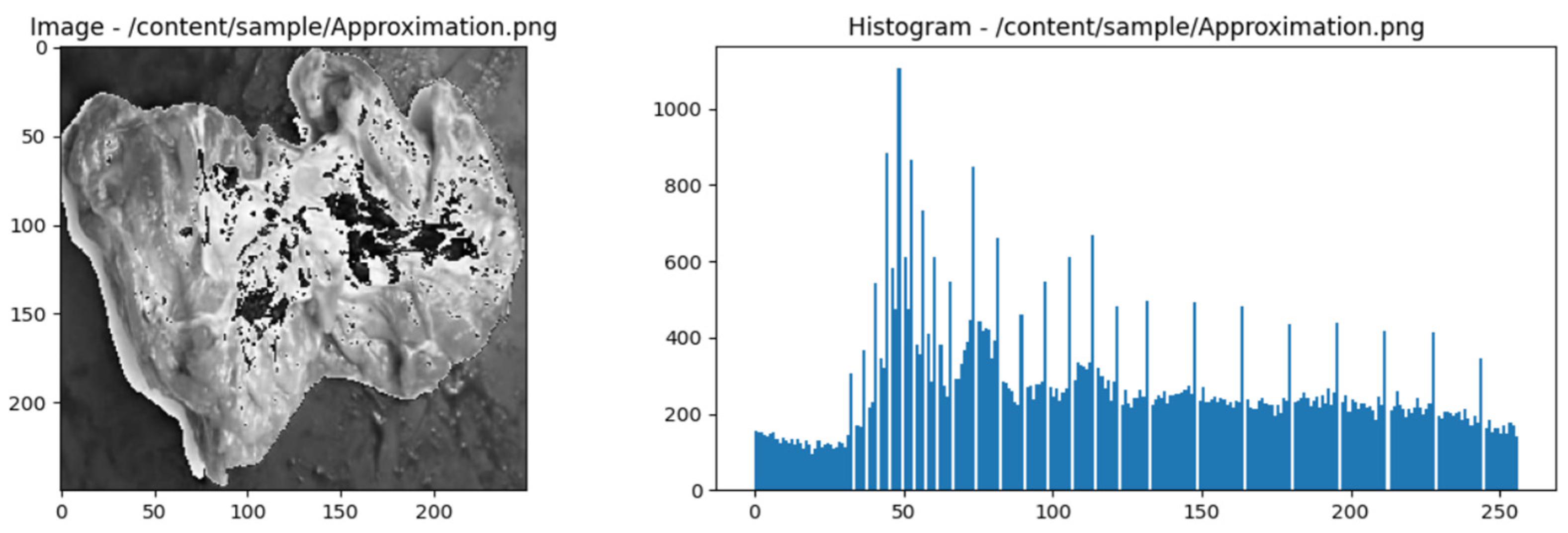
Figure 3.
Approximation Haar wavelet of the image of fresh beef types and histogram.
2.8. Gray Level Co-Occurrence Matrix (GLCM)
Selecting GLCM features is essential for improving sample differentiation. [51]. The Gray Level Co-Occurrence Matrix (GLCM) is a texture analysis tool used in digital image processing. GLCM looks at the spatial connection between grayscale image pixel intensities to extract information about image patterns and textures. GLCM measures the frequency at which pairs of pixels with a given intensity appear together at a given distance and direction. By calculating these matrices and analyzing the texture of meat texture photos, numerous statistics can be produced, such as energy, contrast, correlation, homogeneity, and entropy. For a GLCM element C (i, j) with horizontal direction and distance 1, the general formula is:
Where:
- is the image's pixel intensity at coordinates (m, n).
- is a delta function that returns one if the statement in parentheses is accurate and 0 otherwise.
- M is the number of image rows.
- N is the number of image columns.
Basic GLCM computation for the horizontal direction at a distance of one from the grayscale image that follows:
The calculation steps are as follows:
- Select horizontal direction and distance 1.
-
Count the pairs of pixels that appear together:
- Scan the image to identify pairs of pixels with matching intensities.
- Pixel pairs that appear together are: (1, 1), (1, 2), (2, 3), (3, 4), (2, 2), (3, 3), (4, 4 ), (1, 1), (1, 2), (2, 3), (3, 4), (2, 2), (3, 3), (4, 4).
-
Create GLCM Matrix:
- Count the occurrences of pixel pairs and insert them into the GLCM matrix.
-
GLCM Matrix Normalization:
- Normalize the matrix to obtain a probability distribution.
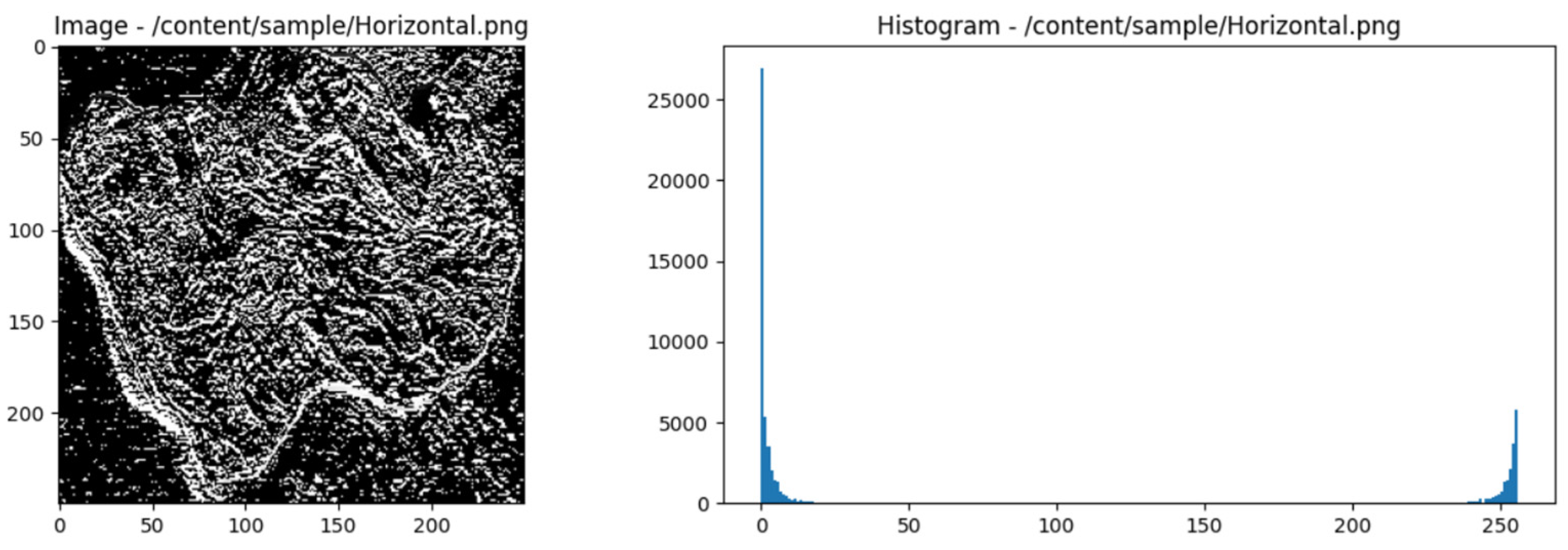
Figure 4.
GLCM horizontal of the image of fresh beef types and histogram.
For a GLCM element C (i, j) with vertical direction and distance 1, the general formula will depend on the definition of the GLCM matrix and the specific direction used. Assume we are working with grayscale images with intensity levels between 0 and where L is the number of intensity levels. The general formula for calculating GLCM elements C (i, j) with vertical direction and distance 1 is:
Where:
- is the image's pixel intensity at coordinates (m, n).
- is a delta function that returns one if the statement in parentheses is accurate and 0 otherwise.
- M is the number of image rows.
- N is the number of image columns.
Simple GLCM calculation for the vertical direction with a distance of 1 from the following grayscale image:
The calculation steps are as follows:
- Select horizontal direction and distance 1.
-
Count the pairs of pixels that appear together:
- Scan the image to identify pairs of pixels with matching intensities.
- Pixel pairs that appear together are: (1, 1), (2, 2), (1, 1), (3, 4), (2, 2), (1, 1), (4, 4), (2, 2), (2, 2), (3, 3), (4, 4), (2, 2), (2, 2), (4, 4).
-
Create GLCM Matrix:
- Count the occurrences of pixel pairs and insert them into the GLCM matrix.
-
GLCM Matrix Normalization:
- Normalize the matrix to obtain a probability distribution.
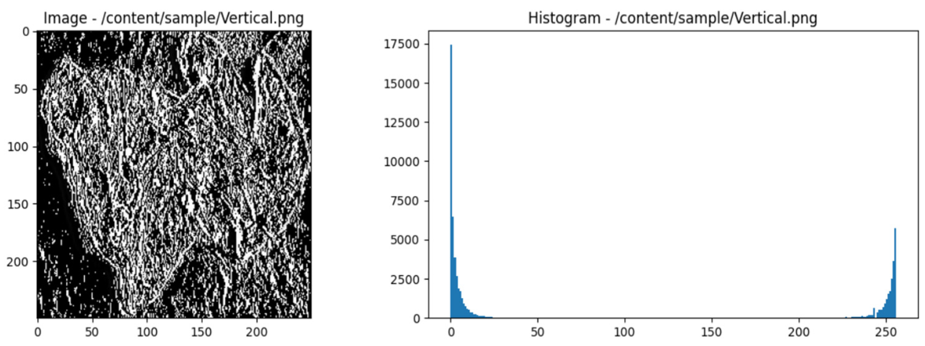
Figure 5.
GLCM vertical of the image of fresh beef types and histogram.
For GLCM elements C (i, j) with diagonal direction and distance 1, the general formula can be formulated as follows:
Where:
- is the image's pixel intensity at coordinates (m, n).
- is a delta function that returns one if the statement in parentheses is accurate and 0 otherwise.
- M is the number of image rows.
- N is the number of image columns.
Simple GLCM calculation for the diagonal direction with a distance of 1 from the following grayscale image:
The calculation steps are as follows:
- Select horizontal direction and distance 1.
-
Count the pairs of pixels that appear together:
- Scan the image to identify pairs of pixels with matching intensities.
- Pixel pairs that appear together are: (1, 1), (1, 1), (2, 2), (3, 3), (2, 2), (3, 3), (4, 4), (1, 1), (1, 1), (2, 2), (3, 3), (2, 2), (3, 3), (4, 4).
-
Create GLCM Matrix:
- Count the occurrences of pixel pairs and insert them into the GLCM matrix.
-
GLCM Matrix Normalization:
- Normalize the matrix to obtain a probability distribution.
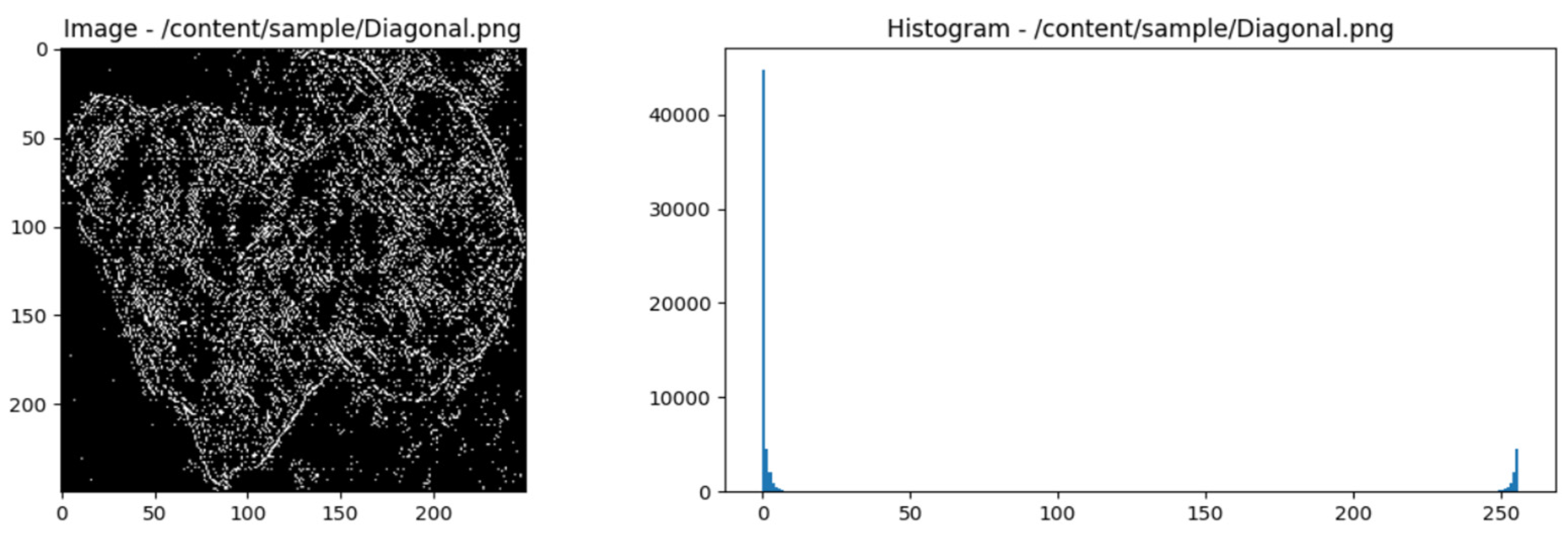
Figure 6.
GLCM diagonal of the image of fresh beef types and histogram.
A clear explanation of how the Gray Level Co-Occurrence Matrix (GLCM) matrix is utilized to explain the relationships between pixels in meat texture photos may be found in your analysis of the GLCM computation stages. Here are a few more points:
-
Direction and Distance SelectionThe selection of direction and distance holds significance as it influences the measurement of the relationship between pixels. This has an impact on the texture information that is taken from the picture.
-
GLCM Matrix CalculationCounting the occurrences of particular pairs of pixel intensities at specific distances and directions is necessary to calculate a GLCM matrix. The end product is a matrix displaying the frequency of particular pairs of pixels occurring together.
-
Matrix NormalizationMatrix normalisation is applied to determine the probability distribution of pixel pair appearances. This probability distribution can calculate the likelihood that a pair of pixels will appear about the image's overall size.
-
Feature Extraction from Matrix NormalizationAfter normalisation, numerous texture properties, including energy, contrast, correlation, homogeneity, and entropy, can be retrieved from the matrix. Every element offers distinct details regarding the textural characteristics of the picture
-
Texture Statistics and CharacteristicsEnergy calculations can see the degree to which pixel intensity approaches a given value. The difference in the intensities of neighbouring pixels is referred to as contrast. The degree of correlation between pixel brightness within a specific distance and direction is reflected in correlation. The degree of uniformity in pixel intensity distribution across the image is known as homogeneity. The degree of uncertainty in the pixel intensity distribution is measured by entropy.
Following these procedures creates a set of attributes that can be utilized to identify or describe meat texture photographs more accurately. This method has several uses in pattern recognition and image analysis, particularly in image processing for meat type identification and classification.
Figure 7.
Texture image classification of types of meat using k-NN, Wavelet Haar, and GLCM approaches.
Figure 7.
Texture image classification of types of meat using k-NN, Wavelet Haar, and GLCM approaches.
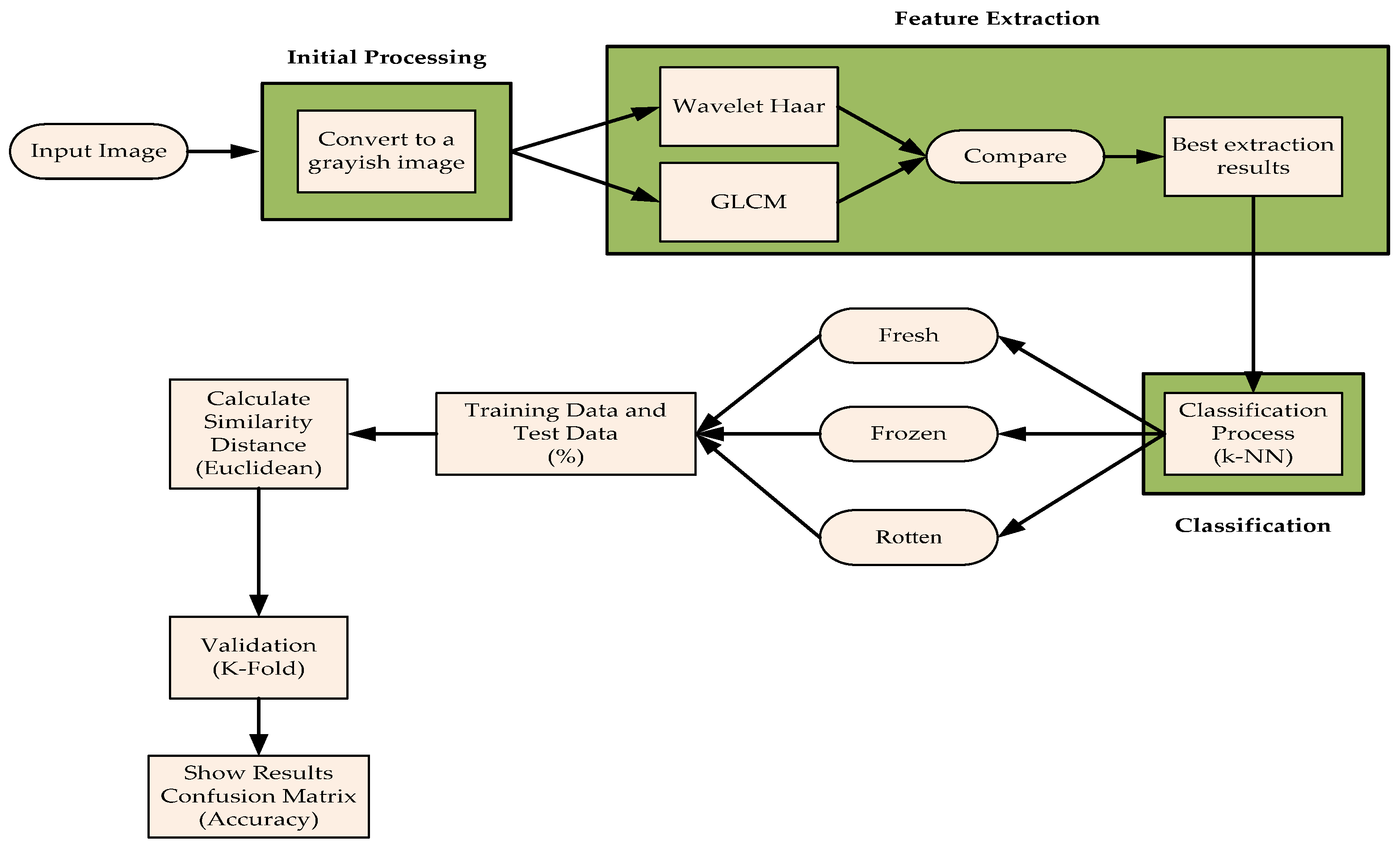
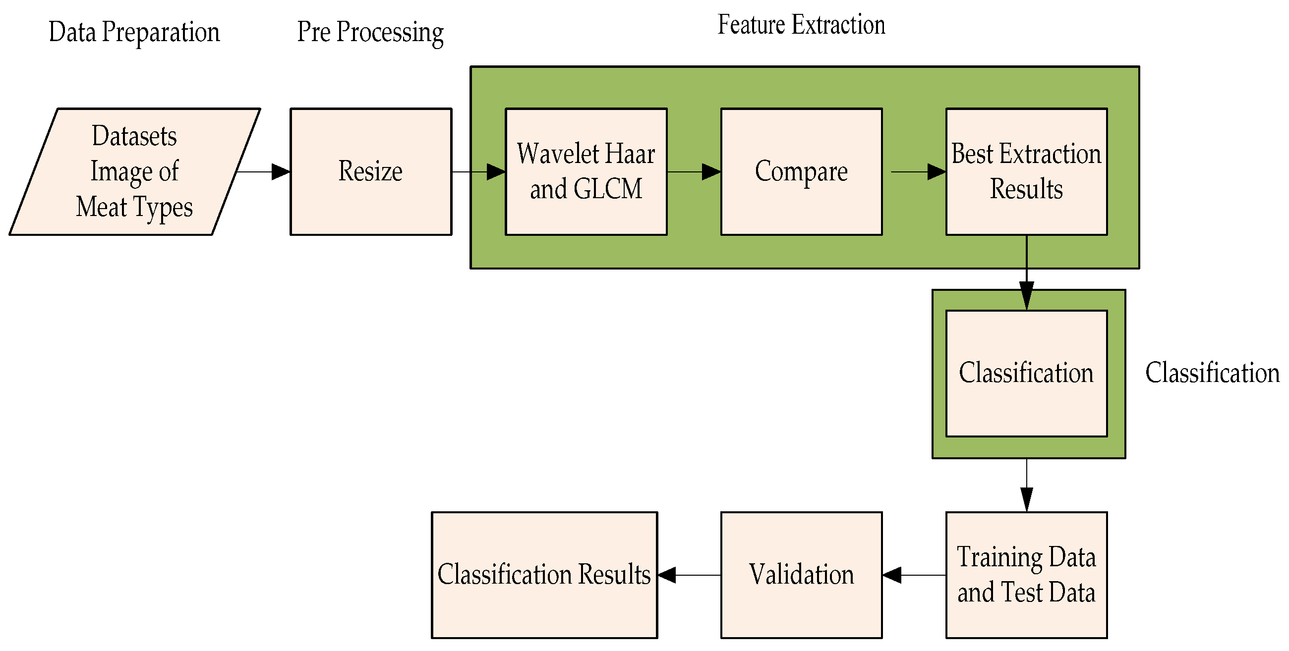
The k-NN, Wavelet Haar, and GLCM methodologies can be used to identify several stages and procedures in the classification of textural photographs of different varieties of meat. First, the colour photos of the various beef types were transformed to grayscale as the first step in the processing procedure. Image decomposition utilizing Haar wavelets with smoothing and reduction on lines and columns constitutes the second feature extraction stage using GLCM and Haar wavelets. Creates four images: HH (detail components), LH, HL, and LL (approximation). Each detailed element's average, standard deviation and tendency are computed statistically on deconstructed images. For every deconstructed image, GLCM normalization produces a normalized GLCM. GLCM analysis, or GLCM, to extract features or textural properties, including energy, contrast, correlation, homogeneity, and entropy, is the third feature extraction method from GLCM. Sorting texture photos of different kinds of meat into fresh, frozen, and rotten categories is the fourth classification procedure. Class or label predictions are made using Euclidean and confusion matrices. The final method involves assessing performance using evaluation metrics, i.e., determining how effectively the model can predict the proper class on test data using measures like accuracy. Its accuracy is how closely a prediction resembles the actual or expected value. The six classification outcomes are based on picture classification. Precisely, fresh, frozen, and rotting are the three categories into which different meat varieties' texture picture categorization findings are divided. Using this method, the model can comprehend and identify patterns or characteristics that distinguish different meat varieties' textures in pictures. Metrics like accuracy are used in performance evaluation to show how effectively the model predicts the proper class on test data. Using the classification results, meat varieties can subsequently be categorized according to their conditions.
2.9. System Implementation and Testing
-
Number of samples and classificationSeven hundred and fifty images show various types of meat textures. Every kind of meat has three categories: fresh, frozen and rotten. There are fifty texture images for each class of beef and 150 images per type of meat.
-
Dataset divisionThe 600 images in the training set and the 150 in the testing set form the two main parts of the dataset. Sharing these datasets is essential so that models can be trained and their performance can be tested objectively.
-
Type of meat testedFive different kinds of meat were tested: pork, goat, horse, buffalo, and beef. Each sort of meat has three texture grades: fresh, frozen, and rotten.
-
Use of digital camerasA digital camera with the same light intensity and distance takes images that form a meat texture data set. This is important to guarantee constant shooting conditions.
-
Image sizeThere are 500x500 pixels in the image. This site offers enough resolution to allow for detailed texture investigation.
-
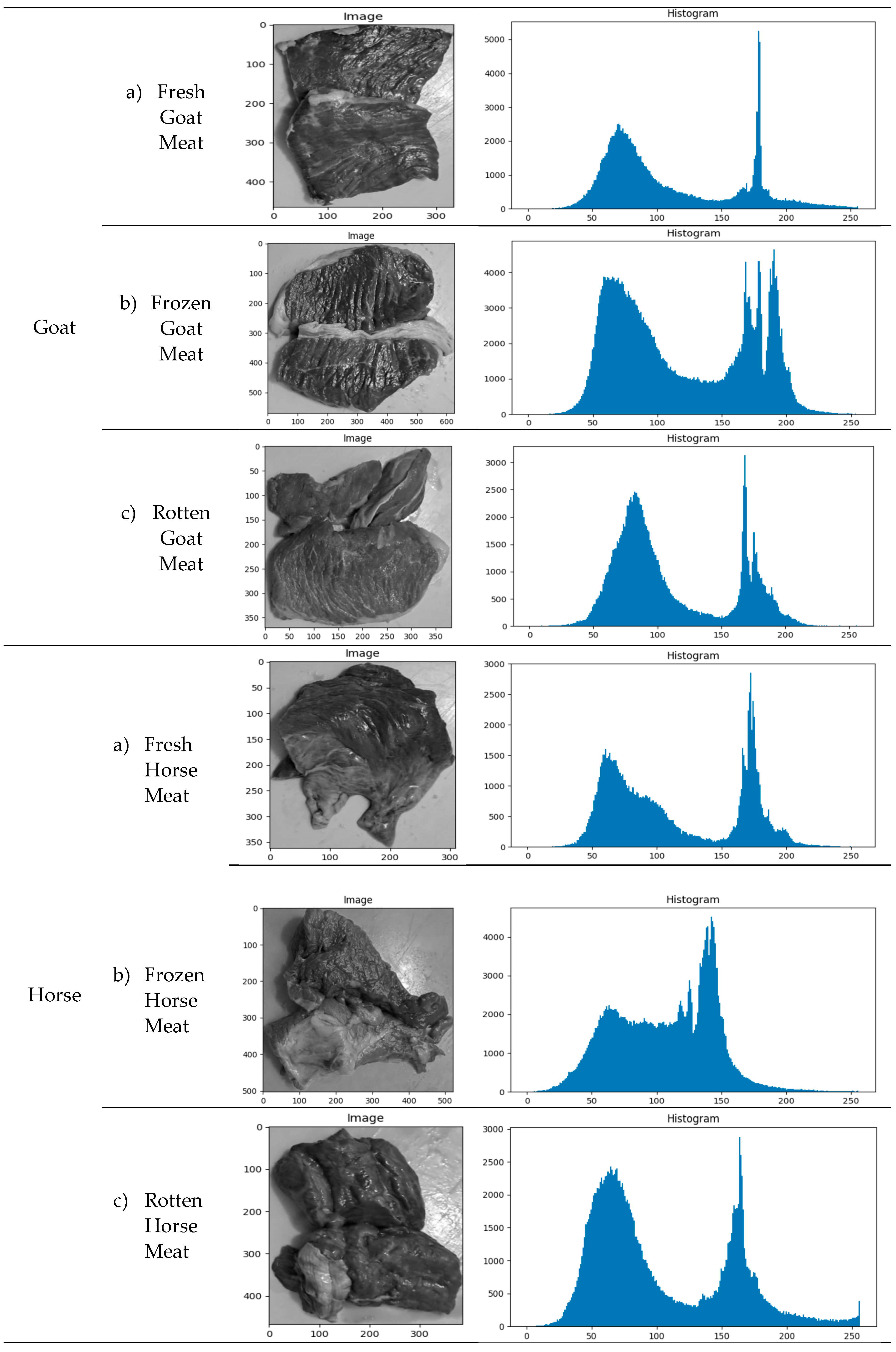
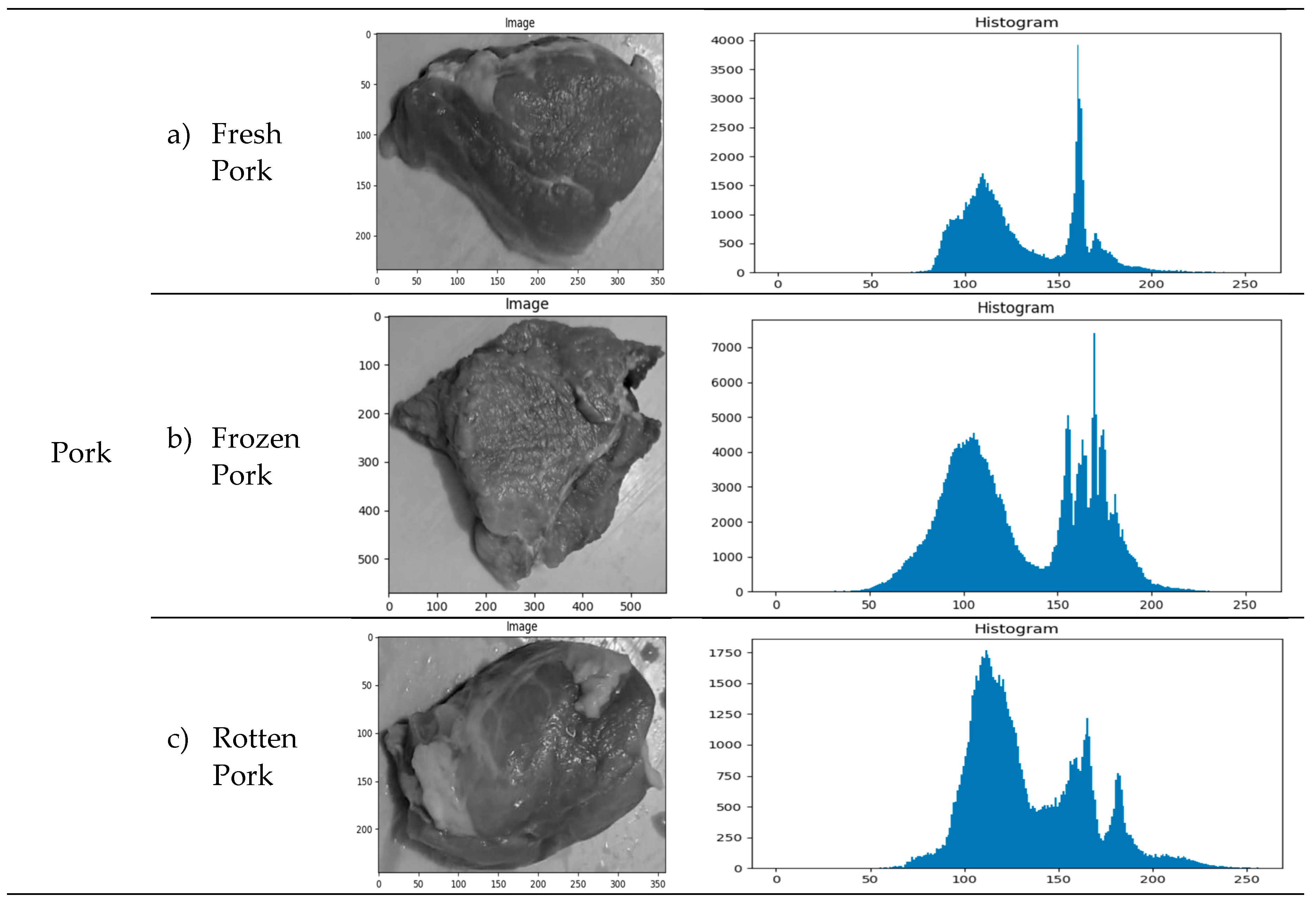
Example of image acquisition resultsExamples of the results of taking texture photos for each class of meat are shown in Table 2. Understanding the range of images tested and used in the categorization process is crucial.
-
Distribution of GLCM ValuesThe distribution of GLCM values based on the meat-type image histogram is shown in Table 2. This examination makes understanding textural characteristics that can be retrieved and applied to the classification process possible.
The implementation and testing of meat-type classification systems have a strong foundation thanks to the experimental setting, which includes well-divided datasets, consistent camera use, and an in-depth examination of the distribution of GLCM values. All of these procedures are crucial to guarantee the classification model's dependability and strong generalization on never-before-seen data (test data).
3.0. Classification
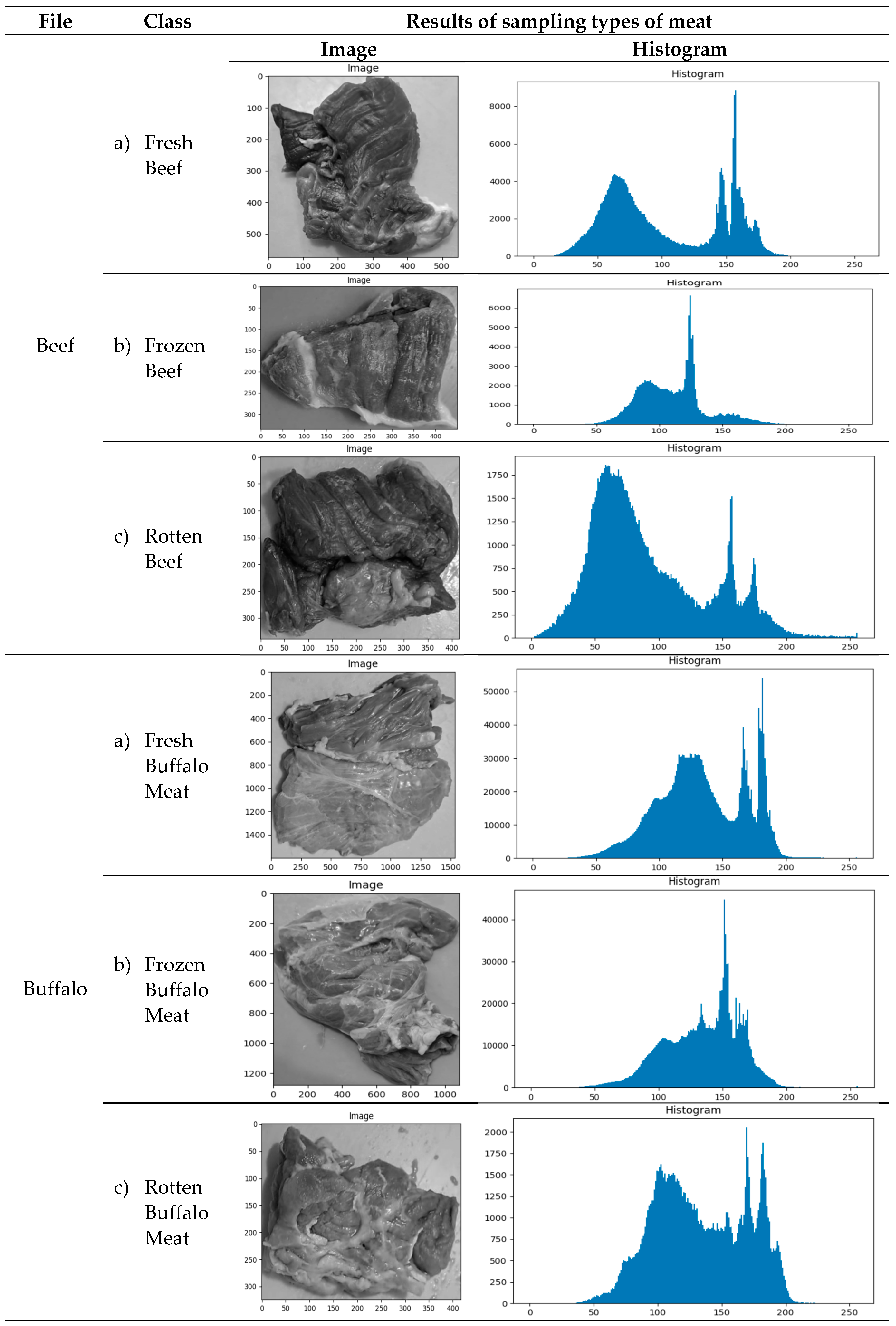
Based on a combination of characteristics, k-nearest neighbour (k-NN) categorization results. Table 2 shows the image of the results of the meat texture experiment related to class (a) fresh meat, class (b) frozen meat, and class (c) rotten meat, as well as the histogram distribution.
As can be seen in Table 7, this study sampled texture photos from five different meat kinds (beef, buffalo, goat, horse, and hog), each of which was available in three other states: fresh, frozen, or rotting. An examination of the tables mentioned is provided below: Starting with beef, there are 150 samples of textural photos available, 50 samples each representing fresh, frozen, and rotting situations. One hundred fifty beef samples in all were used in the investigation. Second, 150 photos showing the texture of buffalo meat—50 samples each for frozen, rotting, and fresh states. For the duration of the investigation, 150 samples of buffalo meat were collected. Goat flesh was the third. Specifically, 150 goat flesh texture image samples were collected: 50 for frozen and 50 for fresh circumstances. For the duration of the investigation, 150 samples of goat flesh were examined. There were 150 texture picture samples total for the four-horse flesh samples—50 for fresh, frozen, and snowy situations. For the duration of the investigation, 150 samples of horse flesh were examined. There were 150 texture picture samples total from the five pig flesh samples, with 50 samples each from fresh, frozen, and rotten states. One hundred fifty pork samples in all were used in the investigation. With 150 samples of each sort of meat, the total sample, or the number of samples for the entire study, was 750. Partitioning the dataset: the 600 samples of training data and the 150 samples of testing data comprise the two halves of the dataset. Research can better depict different meat types and situations by categorizing data in this way. Reliable assessment of the models or techniques applied to feature extraction and analysis of meat texture photos is further supported by the dataset's separation into training and testing subsets.
3.1. Histogram
Figuring out how many pixels are in the image at each intensity level is part of the algorithm used to calculate the histogram. Here's the fundamental formula to calculate the histogram assuming the image is monochromatic or has one intensity level:
For example:
is the number of pixels in the image,
is the number of possible intensity levels (e.g., for a grayscale image, ,
Hence the histogram can be calculated using the formula:
Where:
- is the frequency of occurrence of the pixel intensity to-
- is the number of pixels with intensity to-
- is the total number of pixels in the image.
The result of the calculation above is a normalized value, which indicates that the total of all histogram items is 1. Furthermore, the following formula can be used to get the cumulative histogram:
is the cumulative distribution function for pixel intensities to-
is the histogram value of the pixel intensity to-
The cumulative distribution function represents the proportion of total pixels with an intensity less than or equal to a specific value (PDF). Histogram computations are crucial in several domains, including image processing, colour analysis, and image data processing.
3. Results and Discussion
3.1. Experiment Results
The size of each fresh, frozen, and rotten meat class was confirmed by analyzing 750 meat texture samples from five different types of goat, horse, pork, and beef images. The pixels in each meat image are unique. The absence of scaling when taking meat samples results in variations in pixel size between images. Especially in high-resolution photography, scaling can result in visual distortion, reduced image quality, and increased computational effort [52,53]. Experiments were conducted to ensure that different pixel sizes for each type and meat quality were carefully studied to provide consistency and accuracy in test results and avoid distortion or conflict due to variations in image quality. Based on pixel intensity and pixel frequency, it is simulated that the sample size and histogram distribution in class (a) datasets are, on average, more significant and more dominant than in class (b) and class (c) datasets. The frequency and intensity distribution of pixels in an image, as well as the histogram distribution, determine the image's appearance, and this is the main focus of the analysis performed by various algorithms.

Table 2.
An illustration of the histogram distribution and the meat texture experiment findings for classes (a) fresh meat, class (b) frozen meat, and class (c) rotten meat. There are 50 samples of fresh meat, 50 samples of frozen meat, and 50 samples of rotten meat for each type of meat in each class.
This research K-NN was created using the Google Colab platform. A GPU, or graphics processing unit, was used in each experiment. Two approaches are usually taken. In the first stage, two techniques—GLCM and the Haar wavelet algorithm—are used to extract features used to identify meat images. In the second approach, meat images are determined directly from tracked meat features (feature extraction) using k-NN, which has been trained on various image domains. The feature set is then fed into a k-NN model to see if the classification performance is sufficient to separate texture images (a) from texture images (b) and texture images (c).
3.2. Feature Selection Result
Five different types of meat images, beef, buffalo, goat, horse, and pork, were used to test the feature selection findings. Each type of meat image was classified into three classes: fresh, frozen, and rotten. Each meat is described in Table 3 using GLCM metrics, including homogeneity, contrast, correlation, energy, and entropy. It's crucial to remember that every flesh texture image has the same pixel size, which is 500x500 [56,57]. The choice to employ uniform pixel sizes across all flesh texture images may have been made with an eye toward optimizing computer power. It can lower the computing load and expedite the data analysis process by employing a consistent pixel size. This choice has a number of drawbacks, though, including a lack of spatial resolution and difficulty accurately capturing any scale variations that might exist among the photos. The texture of each meat image can still be learned a great deal by using GLCM metrics, which include contrast, correlation, energy, homogeneity, and entropy. When comparing the textural properties of fresh, frozen, and rotten meat from different kinds of animals under observation, this GLCM measure can be helpful. Thus, despite limitations in spatial resolution, GLCM analysis can still provide valuable insights into meat texture recognition and classification. Therefore, GLCM analysis can still offer valuable insights into the detection and classification of flesh texture despite its limitations in spatial resolution.
Table 3 illustrates how well all feature sets distinguish between the three classes (a), (b), and (c). For fresh meat images, the average ranges from 51.52% to 183.21%, while for frozen meat images, the average ranges from 78.25% to 185.75%. Rotten meat images, on the other hand, have an average range of 34.62% to 115.79%.
The picture of fresh meat demonstrates how fresh pigs have a less diverse texture than other meats. In contrast, higher averages for all recorded GLCM measurements suggest that the intensity variation of fresh goat meat was more significant. Significant variations in the intensity and texture structure of fresh meat images from various meat varieties were shown by this experiment. These differences are crucial for categorizing and identifying pictures and understanding the textural characteristics of various meat kinds.
In the meantime, the frozen meat image reveals that the frozen pork texture image has the lowest average. This indicates that the texture of frozen pig has less variation in intensity than that of frozen goat meat. Frozen goat meat, on the other hand, displayed more notable intensity differences. This report provides a summary of the textural characteristics of frozen goat flesh. This information can be helpful in both learning more about the differences between different slices of meat and identifying or classifying images of frozen beef.
However, the picture of the rotting meat demonstrates that, in most cases, the texture difference between rotten pork and rotten beef is less severe. The intensity difference was more significant for the decaying flesh. This study advances our knowledge of the textural characteristics of pictures of rotting beef. This information can distinguish between various states of meat and identify or classify the stages of rotten meat [58,59].
Table 4 presents the validation results for all aspects of class (a), (b), and (c) using k-NN classification. It is expected that (A) sensitivity, (B) specificity, (C) accuracy, and (D) Matthews correlation function well. For fresh meat images, the coefficients have percentages ranging from (A): 97.959% to 100%; (B): 96.078% to 100%; (C): 97% to 99%; and (D): 94.019% to 98.02%. Meanwhile, images of frozen beef with percentages ranging between 96.078% to 100% in (A), 97.959% to 100% in (B), 97% to 99% in (C), and 94.019% to 98.02% in ( D)). Meanwhile, the percentage of rotten meat images is as follows: (A): 92.308% to 96%; (B): 95.833% to 97.917%; (C): 94% to 96%; and (D): 88.07% to 92.074%) [60,61]. Findings from analyses of (A), (B), (C), and (D) fresh, frozen, and rotten meat images offer essential information about how well k-NN classification models can categorize meat states. Based on the texture image.
Fresh Meat: The model can correctly detect fresh meat images for both categories, as evidenced by (A) having the most significant proportion and being more dominant in fresh goat and fresh horse meat texture images. (B) have different quality percentages. With the highest accuracy images for fresh meat texture, the model can correctly differentiate fresh beef from frozen or rotten beef. This shows how well the model can differentiate fresh meat images from other settings. C) The model can classify fresh meat images correctly; fresh beef and fresh horse meat texture images are the most accurate. This shows how well the model can recognize fresh meat images and differentiate them from other conditions. Images of fresh beef and fresh horse meat (D) are more common in texture images and have the highest percentage (D). This shows a good agreement between the feature model and the actual classes in the fresh meat environment for the classification results. On the other hand, the percentage (D) in the texture image of fresh buffalo meat shows worse performance.
Frozen Meat: The tendency of the model to accurately recognize frozen pork images is demonstrated by the fact that the model has (A) the highest percentage of predominance over frozen buffalo meat texture images. On the other hand, the texture image of frozen buffalo meat has (A) the lowest rate, indicating a problem with identifying frozen buffalo meat. The decreasing tendency of the model to correctly classify frozen buffalo meat photos is shown by (B), which displays the lowest percentage of all frozen buffalo meat texture images. In contrast, the texture images of frozen beef and frozen horse meat received the most significant percentage (B), indicating that the model performs better in accurately classifying these images. (C) The frozen buffalo meat texture image has the lowest accuracy, while the frozen pork texture image has the best dominant accuracy. This shows that the model classifies frozen pork images more accurately than buffalo meat images. However, this algorithm performed very well when classifying frozen meat images. When comparing the texture images of frozen goat meat and frozen pork, the percentage of frozen beef with (D) is the highest. This shows how well and accurately the algorithm can classify texture images of frozen mutton and pork. On the other hand, (D) the percentage of frozen buffalo meat texture images shows worse performance.
Rotting Meat: shows the model's skill in identifying images of rotting goat meat, with (A) the highest percentage being more dominant in texture images. However, in the picture, the texture of rotten buffalo meat has (A) the lowest percentage, so it is challenging to distinguish rotten buffalo meat. (B) has the lowest rate for texture images of rotten buffalo meat and rotten horse meat; this shows the difficulty of effectively recognizing the images of these two types of Meat. However, the texture images of rotten beef and rotten pork have (B) the highest percentage, which shows that the model is more accurate in classifying images of rotten Meat and rotten pork. (C) The texture image of rotten goat meat, rotten pork and rotten buffalo meat has the highest accuracy, while the texture image of rotten beef has the lowest accuracy. This shows that for the model to accurately classify images of rotting buffalo meat, the model must be more precise. However, the images of rotten beef, rotten goat meat, and rotten pork can be recognized correctly through this experiment. But overall, this system works well in categorizing cases of rotting flesh. (D) texture description of rotten pork, rotten goat meat, and rotten beef. Rotten Meat is more common and has the best percentage (D). The model performs well in classifying images of rotting flesh; however, the lowest rate of images was associated with the texture of rotting horse meat (D).
Table 5 shows how well the three models compare in terms of comparison results of performance measurements of the k-nearest neighbor (k-NN) algorithm, the Haar Wavelet algorithm, and the Gray Level Co-occurrence Matrix (GLCM) for the three classes (fresh, frozen, and frozen). Frozen). Rotten). (A) k-NN, (B) Wavelet Haar and (C) GLCM assumed. First, for the fresh meat texture image class, (A): 97% to 99%; (B): 89.25% to 89.96%; and (C): 51.52% to 183.21%. The percentage of frozen meat in both images is 97% to 99% in (A), 87.56% to 88.25% in (B), and 78.25% to 185.75% in (C), third, with the percentage ranges from 94%. Up to 96% in (A), 86.26% to 87.97% in (B), and 34.62% to 115.79% in (C) for the rotting flesh image.
The performance results of algorithms (A), (B), and (C) on fresh, frozen, and rotten meat images provide valuable insight into the performance of algorithm models in determining the condition of Meat based on texture images. Fresh Meat First: (A) The k-NN algorithm gives the best results on texture images of fresh goats, horses and cattle. It also has the most significant standout score (99%). This shows how well the k-NN algorithm performs when classifying fresh meat images. Regarding the texture image of fresh buffalo meat, k-NN has the worst performance, with a score of 97%. Meanwhile, (B) the texture image of fresh pork shows that the performance of the Haar Wavelet algorithm is worse (89.25%) than k-NN. However, when it comes to fresh beef texture images, our algorithm performs well (89.96%). Meanwhile, for the texture image of fresh pork (C), the GLCM method gave inconsistent results, with the lowest application percentage (51.52%). However, GLCM data can still be used for classification. However, GLCM has the most significant proportion of fresh goat meat texture images (183.21%). Of the three algorithms studied, the GLCM, Wavelet Haar, and k-NN models performed the best in categorizing fresh meat texture images into meat categories. This shows that the k-NN technique is more suitable for applications that organize texture images of Fresh Meat.
Second Frozen Meat: (A) Using the k-NN method, the texture image of frozen pork gives the most prominent value (99%), while the texture image of frozen buffalo meat gives the lowest result (97%). This shows how well the k-NN algorithm classifies frozen meat images. However, compared with k-NN, the Haar Wavelet algorithm performs worst (87.56%) on frozen beef texture images. However, the algorithm continues to produce good results. 88.25 per cent) is the highest performance in frozen beef texture images. Based on the GLCM algorithm, the texture image of frozen pork (C) has the lowest value, 78.25%. However, GLCM results can still be used to classify frozen meat images. After three rounds of testing, k-NN maintained its top ranking in frozen meat texture image classification, with Wavelet Haar and GLCM ranking second and third. This shows that applications that require frozen meat texture image classification are more suitable for using the k-NN technique. GLCM was the best model in performance testing, with an accuracy of 185.75%.
Third, Rotten Meat: (A) has the lowest percentage (94%), although the texture images of rotten beef, rotten goat, and rotten pig have the highest k-NN values (96%). This demonstrates how effectively the k-NN algorithm classifies pictures of rotting flesh. While (B) k-NN outperforms the Haar Wavelet algorithm (86.26%), there is an image of decaying buffalo flesh. However, the algorithm continues to yield good results. Conversely, (C) The GLCM approach yields erratic results; the textural image of rotten pork has the lowest performance % (34.62). However, GLCM data can still be used to categorize images of rotting flesh. However, the rotten beef texture image had the highest performance percentage (115.79%). After testing three different algorithms, k-NN, GLCM, and Wavelet, Haar continued to produce the best classification results for images containing rotting meat textures. This shows that when classifying rotting meat texture images, the k-NN approach is more suitable.
Table 6.
Classification accuracy based on meat texture analysis.
| Author | Structure | Texture Analysis Method (Features) | Method | Accuracy (%) |
|---|---|---|---|---|
| Yudhana, Anton Umar, Rusydi Saputra, Sabarudin[36] | Fish | RGB colors and GLCM features | k-NN | 94% |
| Don Africa, Aaron M Claire Alberto, Stephanie T Evan Tan, Travis Y[62] | Beef and pork | Skewness, Kurtosis, Mean, and Std Deviation | k-NN | 98.6% |
| Wijaya, Dedy Rahman Sarno, Riyanarto Zulaika, Enny[63] | beef | Regression results (black: actual, blue: prediction, red: prediction with error | Discrete Wavelets Transform and Long Short-Term Memory (DWTLSTM) dan k-nearest neighbour (k-NN) | 85,05% |
| Kiswanto, Hadiyanto, and Eko Sediyon[2] | Beef, buffalo, goat, horse and pork | RGB, GLCM and HSV | Haar wave algorithm | 76.72% |
| Ayaz, Hamail Ahmad, Muhammad Mazzara, Manuel Sohaib, Ahmed[64] | Meat | HSI | k-NN | 82% |
5. Conclusions
Fresh Meat: With a very high-performance percentage, the k-NN algorithm performs best in categorizing fresh meat texture images, especially fresh goat, horse, and beef textures. However, GLCM also does an excellent job of classifying texture images of fresh meat, especially fresh goat meat. Frozen Meat: With a high percentage of performance on frozen pork texture images, the k-NN algorithm also excels in categorizing frozen meat texture images. In performance testing, GLCM has the advantage because it can classify frozen beef texture images with very high accuracy. Rotting meat: The k-NN algorithm demonstrated its efficacy in this work by again standing out in categorizing texture images of rotting meat. Even so, GLCM can still be used to classify pictures of rotting flesh, but with uncertain results. Based on the comprehensive examination, the k-NN technique is generally more appropriate for applications that classify images of meat texture, particularly when differentiating between fresh, frozen, and rotting meat. However, GLCM also yields some quite impressive results, particularly when it comes to classifying frozen beef. While k-NN and GLCM typically perform better in this scenario, the Haar Wavelet algorithm tends to perform worse despite producing appropriate results.
Author Contributions
H.R.: Conceptualization, Data Curation, Formal Analysis, Investigation, Methodology, Software, Validation, Visualization, Writing—original draft, Writing—review & editing. A.S.: Validation, Visualization, Writing—original draft preparation, Writing—review & editing. D.B.: Funding acquisition, Investigation, Project administration, Resources, Supervision, Validation, Writing—original draft preparation. A.M.: Conceptualization, Methodology, Funding Acquisition, Investigation, Project Administration, Resources, Supervision, Writing—preparatory original draft, Writing—review & editing. All authors have read and approved the published version of the manuscript.
Funding
This research received no external funding.
Acknowledgments
The Information Systems Doctoral Program Graduate School supported this research, as did Diponegoro University and the Atma Luhur Pangkalpinang Institute of Science and Business.
Conflicts of Interest
The authors declare no conflict of interest.
References
- S. Ayu Aisah, A. Hanifa Setyaningrum, L. Kesuma Wardhani, and R. Bahaweres, “Identifying Pork Raw-Meat Based on Color and Texture Extraction Using Support Vector Machine,” 2020 8th Int. Conf. Cyber IT Serv. Manag. CITSM 2020, no. c, 2020. [CrossRef]
- and E. S. Kiswanto, Hadiyanto, Modification of the Haar Wavelet Algorithm for Texture Identification of Types of Meat Using Machine. Springer Nature Singapore, 2024. [CrossRef]
- H. H. H, S. Madenda, and S. Widiyanto, “Comparison of Beef Marbling Segmentation by Experts towards Computational Techniques by Using Jaccard , Dice and Cosine Comparison of Beef Marbling Segmentation by Experts towards Computational Techniques by Using Jaccard , Dice and Cosine,” vol. 12, no. 13, pp. 623–627, 2021.
- H. H. Handayani and A. F. N. Masruriyah, “Determination of beef marbling based on fat percentage for meat quality,” Int. J. Psychosoc. Rehabil., vol. 24, no. 1, pp. 8394–8401, 2020. [CrossRef]
- K. Adi, S. Pujiyanto, O. D. Nurhayati, and A. Pamungkas, “Beef quality identification using color analysis and k-nearest neighbor classification,” Proc. - 2015 4th Int. Conf. Instrumentation, Commun. Inf. Technol. Biomed. Eng. ICICI-BME 2015, pp. 180–184, 2016. [CrossRef]
- S. M. K. Uddin, M. A. M. Hossain, Z. Z. Chowdhury, and M. R. Bin Johan, “Short targeting multiplex PCR assay to detect and discriminate beef, buffalo, chicken, duck, goat, sheep and pork DNA in food products,” Food Addit. Contam. - Part A Chem. Anal. Control. Expo. Risk Assess., vol. 38, no. 8, pp. 1273–1288, 2021. [CrossRef]
- V. Sciences et al., “Review Article Identiication of Diferent Animal Species in Meat and Meat Products: Trends and Advances,” vol. 3, no. 6, pp. 334–346, 2015.
- L. S. Dalsecco, R. M. Palhares, P. C. Oliveira, L. V. Teixeira, M. G. Drummond, and D. A. A. de Oliveira, “A Fast and Reliable Real-Time PCR Method for Detection of Ten Animal Species in Meat Products,” J. Food Sci., vol. 83, no. 2, pp. 258–265, 2018. [CrossRef]
- Y. C. Li et al., “Comparative review and the recent progress in detection technologies of meat product adulteration,” Compr. Rev. Food Sci. Food Saf., vol. 19, no. 4, pp. 2256–2296, 2020. [CrossRef]
- M. A. M. Hossain et al., “Quantitative Tetraplex Real-Time Polymerase Chain Reaction Assay with TaqMan Probes Discriminates Cattle, Buffalo, and Porcine Materials in Food Chain,” J. Agric. Food Chem., vol. 65, no. 19, pp. 3975–3985, 2017. [CrossRef]
- F. M. Albkosh, M. S. Hitam, W. N. J. H. Wan Yussof, A. A. K. Abdul Hamid, and R. Ali, “Optimization of discrete wavelet transform features using artificial bee colony algorithm for texture image classification,” Int. J. Electr. Comput. Eng., vol. 9, no. 6, pp. 5253–5262, 2019. [CrossRef]
- X. Sun et al., “Predicting beef tenderness using color and multispectral image texture features,” Meat Sci., vol. 92, no. 4, pp. 386–393, 2012. [CrossRef]
- P. Jackman, D. W. Sun, P. Allen, N. A. Valous, F. Mendoza, and P. Ward, “Identification of important image features for pork and turkey ham classification using colour and wavelet texture features and genetic selection,” Meat Sci., vol. 84, no. 4, pp. 711–717, 2010. [CrossRef]
- M. M. Ávila et al., “Magnetic Resonance Imaging, texture analysis and regression techniques to non-destructively predict the quality characteristics of meat pieces,” Eng. Appl. Artif. Intell., vol. 82, no. March, pp. 110–125, 2019. [CrossRef]
- L. Chen, “Accepted manuscript to appear in IJWMIP Accepted Manuscript International Journal of Wavelets, Multiresolution and Information Processing,” 2017. [CrossRef]
- R. Wijaya, “Noise filtering framework for electronic nose signals: An application for beef quality monitoring,” Comput. Electron. Agric., vol. 157, pp. 305–321, 2019. [CrossRef]
- M. Kishore, A. Issac, N. Minhas, and B. Sarkar, “Image processing based method to assess fi sh quality and freshness,” J. Food Eng., vol. 177, pp. 50–58, 2016. [CrossRef]
- H. Pu, A. Xie, D. W. Sun, M. Kamruzzaman, and J. Ma, “Application of Wavelet Analysis to Spectral Data for Categorization of Lamb Muscles,” Food Bioprocess Technol., vol. 8, no. 1, pp. 1–16, 2015. [CrossRef]
- M. Masoumi, M. Marcoux, L. Maignel, and C. Pomar, “Weight prediction of pork cuts and tissue composition using spectral graph wavelet,” J. Food Eng., vol. 299, no. January, p. 110501, 2021. [CrossRef]
- R. Wijaya, R. Sarno, E. Zulaika, and S. I. Sabila, “Development of mobile electronic nose for beef quality monitoring,” Procedia Comput. Sci., vol. 124, pp. 728–735, 2017. [CrossRef]
- K. Song, S. hui Wang, D. Yang, and T. yu Shi, “Combination of spectral and image information from hyperspectral imaging for the prediction and visualization of the total volatile basic nitrogen content in cooked beef,” J. Food Meas. Charact., vol. 15, no. 5, pp. 4006–4020, 2021. [CrossRef]
- I.G. Sujana and E. Putra, “Classification of Tuna Meat Grade Quality Based on Color Space Using Wavelet and k-Nearest Neighbor Algorithm,” no. November, pp. 2–4, 2023.
- V. Amin, D. Wilson, G. Rouse, and S. Udpa, “Multiresoi , Utional Texture Analysis for Ultrasound Tissue,” vol. 14, pp. 201–215, 1998.
- Y. Tao, “Wavelet-based adaptive thresholding method for image segmentation,” Opt. Eng., vol. 40, no. 5, p. 868, 2001. [CrossRef]
- M. K. Dutta, A. Issac, N. Minhas, and B. Sarkar, “Image processing based method to assess fish quality and freshness,” J. Food Eng., vol. 177, pp. 50–58, 2016. [CrossRef]
- N. D. Kim, V. Amin, D. Wilson, G. Rouse, and S. Udpa, “Ultrasound image texture analysis for characterizing intramuscular fat content of live beef cattle,” Ultrason. Imaging, vol. 20, no. 3, pp. 191–205, 1998. [CrossRef]
- R. A. Asmara et al., “Classification of pork and beef meat images using extraction of color and texture feature by Grey Level Co-Occurrence Matrix method,” IOP Conf. Ser. Mater. Sci. Eng., vol. 434, no. 1, 2018. [CrossRef]
- S. Widiyanto, “Texture Feature Extraction Based On GLCM and DWT for Beef Tenderness Classification,” 2018 Third Int. Conf. Informatics Comput., pp. 1–4.
- R. A. Asmara et al., “Chicken meat freshness identification using colors and textures feature,” 2018 Jt. 7th Int. Conf. Informatics, Electron. Vis. 2nd Int. Conf. Imaging, Vis. Pattern Recognition, ICIEV-IVPR 2018, pp. 93–98, 2019. [CrossRef]
- M. M. Santoni, D. I. Sensuse, A. M. Arymurthy, and M. I. Fanany, “Cattle Race Classification Using Gray Level Co-occurrence Matrix Convolutional Neural Networks,” Procedia Comput. Sci., vol. 59, no. Iccsci, pp. 493–502, 2015. [CrossRef]
- M. E.-H. . H. M. E. . H. M. . & N. M. Ibrahim, “Muzzle feature extraction based on gray level co-occurrence matrix,” Isr. J. Vet. Med., vol. 01, pp. 16–24, 2016.
- R. Farinda, Z. Firmansyah, C. Sulton, I. G. P. S. Wijaya, and F. Bimantoro, “Beef Quality Classification based on Texture and Color Features using SVM Beef Quality Classification based on Texture and Color Features using SVM Classifier,” no. September, 2018. [CrossRef]
- S. Agustin and R. Dijaya, “Beef Image Classification using K-Nearest Neighbor Algorithm for Identification Quality and Freshness,” J. Phys. Conf. Ser., vol. 1179, no. 1, 2019. [CrossRef]
- B. Jia, W. Wang, S. C. Yoon, H. Zhuang, and Y. F. Li, “Using a combination of spectral and textural data to measure water-holding capacity in fresh chicken breast fillets,” Appl. Sci., vol. 8, no. 3, 2018. [CrossRef]
- S. Suhadi, P. Dina Atika, S. Sugiyatno, A. Panogari, R. Trias Handayanto, and H. Herlawati, “Mobile-based fish quality detection system using k-nearest neighbors method,” 2020 5th Int. Conf. Informatics Comput. ICIC 2020, 2020. [CrossRef]
- A.Yudhana, R. Umar, and S. Saputra, “Fish Freshness Identification Using Machine Learning: Performance Comparison of k-NN and Naïve Bayes Classifier,” J. Comput. Sci. Eng., vol. 16, no. 3, pp. 153–164, 2022. [CrossRef]
- H. Jiang, W. Yuan, Y. Ru, Q. Chen, J. Wang, and H. Zhou, “Feasibility of identifying the authenticity of fresh and cooked mutton kebabs using visible and near-infrared hyperspectral imaging,” Spectrochim. Acta - Part A Mol. Biomol. Spectrosc., vol. 282, no. July, 2022. [CrossRef]
- A.P. A. da C. Barbon et al., “Development of a flexible Computer Vision System for marbling classification,” Comput. Electron. Agric., vol. 142, no. November, pp. 536–544, 2017. [CrossRef]
- S. I. Sabilla, R. Sarno, K. Triyana, and K. Hayashi, “Deep learning in a sensor array system based on the distribution of volatile compounds from meat cuts using GC–MS analysis,” Sens. Bio-Sensing Res., vol. 29, no. July, 2020. [CrossRef]
- J. A. Matera et al., “Discrimination of Brazilian artisanal and inspected pork sausages: Application of unsupervised, linear and non-linear supervised chemometric methods,” Food Res. Int., vol. 64, pp. 380–386, 2014. [CrossRef]
- T. Gaber, A. Tharwat, A. E. Hassanien, and V. Snasel, “Biometric cattle identification approach based on Weber’s Local Descriptor and AdaBoost classifier,” Comput. Electron. Agric., vol. 122, pp. 55–66, 2016. [CrossRef]
- Y. Xiong et al., “Non-Destructive Detection of Chicken Freshness Based on Electronic Nose Technology and Transfer Learning,” Agric., vol. 13, no. 2, 2023. [CrossRef]
- A. González-Mohino, T. Pérez-Palacios, T. Antequera, J. Ruiz-Carrascal, L. S. Olegario, and S. Grassi, “Monitoring the processing of dry fermented sausages with a portable NIRS device,” Foods, vol. 9, no. 9, pp. 1–12, 2020. [CrossRef]
- A. Varghese, S. Jain, M. Jawahar, and A. A. Prince, “Auto-pore segmentation of digital microscopic leather images for species identification,” Eng. Appl. Artif. Intell., vol. 126, no. PC, p. 107049, 2023. [CrossRef]
- V. Fernández-Ibáñez, T. Fearn, A. Soldado, and B. de la Roza-Delgado, “Development and validation of near infrared microscopy spectral libraries of ingredients in animal feed as a first step to adopting traceability and authenticity as guarantors of food safety,” Food Chem., vol. 121, no. 3, pp. 871–877, 2010. [CrossRef]
- S. Kumar, S. K. Singh, R. Singh, and A. K. Singh, “Animal biometrics: Techniques and applications,” Anim. Biometrics Tech. Appl., pp. 1–243, 2018. [CrossRef]
- T. Chen, X. Qi, M. Chen, and B. Chen, “Gas Chromatography-Ion Mobility Spectrometry Detection of Odor Fingerprint as Markers of Rapeseed Oil Refined Grade,” J. Anal. Methods Chem., vol. 2019, 2019. [CrossRef]
- Najam ul Hasan, N. Ejaz, W. Ejaz, and H. S. Kim, “Meat and fish freshness inspection system based on odor sensing,” Sensors (Switzerland), vol. 12, no. 11, pp. 15542–15557, 2012. [CrossRef]
- A.V. Shik et al., “Rapid Testing of Irradissation Dose in Beef and Potatoes by Reaction-Based Optical Sensing Technique,” J. Food Compos. Anal., vol. 127, no. August 2023, p. 105946, 2023. [CrossRef]
- Z. S. Jiang, Rongchang, Rongchang Jiang, Jingxin Shen, Xinran Li, Rui Gao, Qinghe Zhao, “Detection and recognition of veterinary drug residues in beef using hyperspectral discrete wavelet transform and deep learning,” Int. J. Agric. Biol. Eng., vol. 15, no. 1, pp. 224–232, 2022. [CrossRef]
- C. Malegori, L. Franzetti, R. Guidetti, E. Casiraghi, and R. Rossi, “GLCM , an image analysis technique for early detection of bio fi lm,” J. Food Eng., vol. 185, pp. 48–55, 2016. [CrossRef]
- P. P. S. Parsania and D. P. V.Virparia, “A Review: Image Interpolation Techniques for Image Scaling,” Int. J. Innov. Res. Comput. Commun. Eng., vol. 02, no. 12, pp. 7409–7414, 2015. [CrossRef]
- Fedorov, T. Utkina, O. Nechyporenko, and Y. Korpan, “Development of technique for face detection in image based on binarization, scaling and segmentation methods,” Eastern-European J. Enterp. Technol., vol. 1, no. 9–103, pp. 23–31, 2020. [CrossRef]
- C. DeCarli, D. G. M. Murphy, D. Teichberg, G. Campbell, and G. S. Sobering, “Local histogram correction of MRI spatially dependent image pixel intensity nonuniformity,” J. Magn. Reson. Imaging, vol. 6, no. 3, pp. 519–528, 1996. [CrossRef]
- S. H. Bae and M. Kim, “A novel SSIM index for image quality assessment using a new luminance adaptation effect model in pixel intensity domain,” 2015 Vis. Commun. Image Process. VCIP 2015, pp. 5–8, 2015. [CrossRef]
- J. J. Ã and W. C. Ro, “Data processing and image reconstruction methods for pixel detectors The first transmission radiogram was measured by,” vol. 576, pp. 223–234, 2007. [CrossRef]
- H. Wu and Z. Li, “Scale Issues in Remote Sensing: A Review on Analysis, Processing and Modeling,” pp. 1768–1793, 2009. [CrossRef]
- Y. Yang, W. Wang, H. Zhuang, S. C. Yoon, and H. Jiang, “Fusion of spectra and texture data of hyperspectral imaging for the prediction of the water-holding capacity of fresh chicken breast filets,” Appl. Sci., vol. 8, no. 4, 2018. [CrossRef]
- B. Park, M. Kise, W. R. Windham, K. C. Lawrence, and S. C. Yoon, “Textural analysis of hyperspectral images for improving contaminant detection accuracy,” Sens. Instrum. Food Qual. Saf., vol. 2, no. 3, pp. 208–214, 2008. [CrossRef]
- N. Ali, D. Neagu, and P. Trundle, “Evaluation of k - nearest neighbour classifier performance for heterogeneous data sets,” SN Appl. Sci., no. September, 2019. [CrossRef]
- A.J. Gallego, J. R. Rico-juan, and J. J. Valero-mas, “Efficient k -nearest neighbor search based on clustering and adaptive k values,” Pattern Recognit., vol. 122, p. 108356, 2022. [CrossRef]
- A.M. Don Africa, S. T. Claire Alberto, and T. Y. Evan Tan, “Development of a portable electronic device for the detection and indication of fireworks and firecrackers for security personnel,” Indones. J. Electr. Eng. Comput. Sci., vol. 19, no. 3, pp. 1194–1203, 2020. [CrossRef]
- D.R. Wijaya, R. Sarno, and E. Zulaika, “DWTLSTM for electronic nose signal processing in beef quality monitoring,” Sensors Actuators, B Chem., vol. 326, no. September 2020, p. 128931, 2021. [CrossRef]
- H. Ayaz, M. Ahmad, M. Mazzara, and A. Sohaib, “Hyperspectral imaging for minced meat classification using nonlinear deep features,” Appl. Sci., vol. 10, no. 21, pp. 1–13, 2020. [CrossRef]
Table 1.
Confusion Matrix.
| Classification | |||
|---|---|---|---|
| Positive | Negative | ||
| Actual Classification | Positive | TP | FN |
| Negative | FP | TN | |
Table 7.
Feature subsets.
| No | Type of meat | Feature Subsets | Sample |
|---|---|---|---|
| 1 | Beef | Fresh Beef | 50 |
| Frozen Beef | 50 | ||
| Rotten Beef | 50 | ||
| 2 | Buffalo | Fresh Buffalo Meat | 50 |
| Frozen Buffalo Meat | 50 | ||
| Rotten Buffalo Meat | 50 | ||
| 3 | Goat | Fresh Goat Meat | 50 |
| Frozen Goat Meat | 50 | ||
| Rotten Goat Meat | 50 | ||
| 4 | Horse | Fresh Horse Meat | 50 |
| Frozen Horse Meat | 50 | ||
| Rotten Horse Meat | 50 | ||
| 5 | Pork | Fresh Pork | 50 |
| Frozen Pork | 50 | ||
| Rotten Pork | 50 |
Table 3.
Comparison of GLCM feature extraction results for contrast, correlation, energy, homogeneity, entropy metrics.
Table 3.
Comparison of GLCM feature extraction results for contrast, correlation, energy, homogeneity, entropy metrics.
| Type of meat | Class | Metrics GLCM | Minimal | Maximum | Average | ||||
|---|---|---|---|---|---|---|---|---|---|
| Contrast | Correlation | Energy | Homogeneity | Entropy | |||||
| Beef | Fresh Beef | 686,14 | 0,466 | 0,016 | 0,055 | -72,23 | -72,23 | 686,14 | 122,89 |
| Frozen Beef | 552,35 | 0,454 | 0,014 | 0,063 | -72,15 | -72,15 | 552,35 | 96,15 | |
| Rotten Beef | 651,1 | 0,86 | 0,014 | 0,058 | -73,09 | -73,09 | 651,1 | 115,79 | |
| Buffalo | Fresh Buffalo Meat | 656,57 | 0,68 | 0,01 | 0,056 | -72,66 | -72,66 | 656,57 | 116,93 |
| Frozen Buffalo Meat | 551,83 | 0,644 | 0,012 | 0,056 | -73,53 | -73,53 | 551,83 | 95,80 | |
| Rotten Buffalo Meat | 583,98 | 0,056 | 0,018 | 0,053 | -72,43 | -72,43 | 583,98 | 102,33 | |
| Goat | Fresh Goat Meat | 988,17 | 0,28 | 0,015 | 0,056 | -72,48 | -72,48 | 988,17 | 183,21 |
| Frozen Goat Meat | 999,097 | 0,474 | 0,012 | 0,05 | -70,90 | -70,90 | 999,097 | 185,75 | |
| Rotten Goat Meat | 545,43 | 0,304 | 0,017 | 0,064 | -71,60 | -71,60 | 545,43 | 94,84 | |
| Horse | Fresh Horse Meat | 716,54 | 0,278 | 0,012 | 0,055 | -72,82 | -72,82 | 716,54 | 128,81 |
| Frozen Horse Meat | 624,06 | 0,488 | 0,013 | 0,06 | -73,25 | -73,25 | 624,06 | 110,28 | |
| Rotten Horse Meat | 458,32 | 0,332 | 0,02 | 0,079 | -72,17 | -72,17 | 458,32 | 77,32 | |
| Pork | Fresh Pork | 329,53 | 0,376 | 0,025 | 0,056 | -72,37 | -72,37 | 329,53 | 51,52 |
| Frozen Pork | 462,78 | 0,392 | 0,024 | 0,051 | -71,99 | -71,99 | 462,78 | 78,25 | |
| Rotten Pork | 244,98 | 0,34 | 0,029 | 0,064 | -72,30 | -72,30 | 244,98 | 34,62 | |
Table 4.
Validation results using k-NN classification for all class (a), class (b), and class (c) features.
Table 4.
Validation results using k-NN classification for all class (a), class (b), and class (c) features.
| Number of neighbors (k) | Class | Sensitivity | Specificity | Accuracy | Matthews Correlation Coefficient |
|---|---|---|---|---|---|
| 1 | Fresh Beef | 98.039% | 100% | 99% | 98.02% |
| Frozen Beef | 96.154% | 100% | 98% | 96.077% | |
| Rotten Beef | 94.231% | 97.917% | 96% | 92.074% | |
| 2 | Fresh Buffalo Meat | 97.959% | 96.078% | 97% | 94.019% |
| Frozen Buffalo Meat | 96.078% | 97.959% | 97% | 94.019% | |
| Rotten Buffalo Meat | 92.308% | 95.833% | 94% | 88.07% | |
| 3 | Fresh Goat Meat | 100% | 98.039% | 99% | 98.02% |
| Frozen Goat Meat | 98% | 98% | 98% | 98% | |
| Rotten Goat Meat | 96% | 96% | 96% | 92% | |
| 4 | Fresh Horse Meat | 100% | 98.939% | 99% | 98.02% |
| Frozen Horse Meat | 96.154% | 100% | 98% | 96.077% | |
| Rotten Horse Meat | 94.118% | 95.918% | 95% | 90.018% | |
| 5 | Fresh Pork | 98% | 98% | 98% | 96% |
| Frozen Pork | 100% | 98.039% | 99% | 98.02% | |
| Rotten Pork | 94.231% | 97.917% | 96% | 92.074% |
Table 5.
Comparison results of performance measurements of the k-nearest neighbor (k-NN) algorithm, the Haar Wavelet algorithm, and the Gray Level Co-occurrence Matrix (GLCM).
Table 5.
Comparison results of performance measurements of the k-nearest neighbor (k-NN) algorithm, the Haar Wavelet algorithm, and the Gray Level Co-occurrence Matrix (GLCM).
| File | Class | k-NN Accuracy % |
Haar Wavelet Accuracy % |
GLCM Accuracy % |
| Beef | Fresh Beef | 99 | 89,96 | 122,89 |
| Frozen Beef | 98 | 88,25 | 96,15 | |
| Rotten Beef | 96 | 87,97 | 115,79 | |
| Buffalo | Fresh Buffalo Meat | 97 | 89,75 | 116,93 |
| Frozen Buffalo Meat | 97 | 87,96 | 95,80 | |
| Rotten Buffalo Meat | 94 | 86,88 | 102,33 | |
| Goat | Fresh Goat Meat | 99 | 89,47 | 183,21 |
| Frozen Goat Meat | 98 | 86,73 | 185,75 | |
| Rotten Goat Meat | 96 | 86,79 | 94,84 | |
| Horse | Fresh Horse Meat | 99 | 89,85 | 128,81 |
| Frozen Horse Meat | 98 | 87,56 | 110,28 | |
| Rotten Horse Meat | 95 | 86,26 | 77,32 | |
| Pork | Fresh Pork | 98 | 89,25 | 51,52 |
| Frozen Pork | 99 | 87,67 | 78,25 | |
| Rotten Pork | 96 | 86,36 | 34,62 |
Disclaimer/Publisher’s Note: The statements, opinions and data contained in all publications are solely those of the individual author(s) and contributor(s) and not of MDPI and/or the editor(s). MDPI and/or the editor(s) disclaim responsibility for any injury to people or property resulting from any ideas, methods, instructions or products referred to in the content. |
© 2024 by the authors. Licensee MDPI, Basel, Switzerland. This article is an open access article distributed under the terms and conditions of the Creative Commons Attribution (CC BY) license (http://creativecommons.org/licenses/by/4.0/).
Copyright: This open access article is published under a Creative Commons CC BY 4.0 license, which permit the free download, distribution, and reuse, provided that the author and preprint are cited in any reuse.


