
Submitted:
04 April 2024
Posted:
05 April 2024
You are already at the latest version
Abstract
Viscoelastic relaxation measurements on Stirene-Butadiene rubbers (SBR) doped with Carbon Nanotube (CNT) at different concentration show the time-temperature superposition (TTS). This process is described in terms of the Mode Coupling Theory (MCT) approaches to the viscoelasticity by considering the frequency behavior of the loss modulus E”(ω), and shown that the corresponding TTS is linked to a (ω)1/2 decay. From of the analysis of the obtained data we observe that the interaction between the SBR and CNT determine different decays different decays according to their concentration. The rubbers with the lowest CNT concentration are only characterized, in the studied T-range, by a fragile glass forming behavior. Whereas those at the highest ones instead show, at a specific temperature TL, a crossover towards a pure Arrhenius, that according to the MCT, indicates the presence of a kinetic glass transition (KGT); where the system response functions are characterized by scaling behaviors.
Keywords:
viscoelasticity
; relaxations
; polymeric gels
; dynamical arrest
1. Introduction
Liquids approaching transitions characterized by dynamic slowing down, like the sol-gel (typical of polymeric systems and solutions) or the liquid-glass, have together with the very long relaxation times, very high viscosities if compared to, e.g., room-temperature water. The investigation of these highly viscous materials is fascinating because ”independent of their chemical nature of the intermolecular bonds" they share a number of common features [1,2,3,4,5,6,7,8,9,10,11,12,13]. The most significant are a non-Arrhenius temperature dependence of the average relaxation time (before the transition), the non-Debye linear response functions, the energy landscape configuration and a fragile (non-Arrhenius) to strong (Arrhenius) dynamic crossover (FSDC). I.e. a change from a Vogel to an Arrhenius behavior at the temperature , observed by decreasing T and located before the dynamic arrest or transition glass temperature .
Linear response experiments are usually reported in terms of the frequency dependence (or alternatively the time) of the imaginary part (loss contribution) of the response function (susceptibilities) . When the shape of the loss peak in a log-log plot is T independent the liquid obeys to a time-temperature scaling (the so called time-temperature superposition principle or TTS), with respect to the response function. Mathematically, if T is temperature and is the average relaxation time, TTS is obeyed whenever functions N and exist such that .
It has been established that the TTS represents a useful tool for estimating changes in properties of polymer materials at long time or extreme temperatures. In particular, the viscoelastic behaviors of these systems show both time and temperature dependences not only above the glass temperature , but also below. Basically, TTS is related to the concept of equivalence between T and ; under these conditions it is possible to establish simple temperature functions that enable to translate isothermal segments of the considered response function (e.g. the elastic modulus) along the time scale and compose a master curve, registered as a reference temperature () [14].
When TTS applies, response functions are easily determined over many decades of frequency and the procedure works even if some decades are experimentally accessible. The T-shifting function, also called shifting factor, can be described by the Williams-Lendel-Ferry (WLF) equation for systems near and above [15,16] or Arrhenius type equation below it () [14]. It should be noted that the WLF is equivalent to the Vogel-Fulcher-Tamman-Hesse equation (VFTH) [17,18,19].
Despite the fact that TTS has been used intensively over the years it is not universal. TTS violations were not just exceptions for molecular liquids but, in fact, quite common. It has been initially assumed that these violations were due to the interference effects between relaxation process (e.g. and . With the relaxation often found at frequencies higher than those of the dominant relaxation. Nowadays, it is established that the process usually itself violates TTS. For these reasons, although for polymers it has been used continuously until now, there has been little interest in TTS for non-polymeric viscous liquids close to .
However, there is a strong connection between TTS and the Mode-Coupling theory, widely used by the scientific community to explain the dynamics and relaxation functions of glass forming materials in terms of accurate scaling laws. In the less viscous regime at higher temperatures where MCT is believed to apply, this theory’s TTS prediction has received some confirmation from both experiment and computer simulations [9]. From the MCT perspective, breakdowns of TTS in the very high viscosity regime correlates with the well-known breakdown of ideal MCT formalism.
This paper addresses in the behavior of highly viscous liquids (near ) and the motivation for reinvestigating the validity of TTS in this regime by integrating it with the general MCT approaches for the viscoelasticity. In particular, we have followed a suggestion proposed by a study, done on molecular liquids, dedicated to verifying the general validity of the TTS in thermodynamic conditions such that the two main relaxations ( and ) have no influence on each other [20]. In particular, this study, dealing with the data of on supercooled triphenyl phosphate (and other molecular liquids close to the calorimetric glass transition), shows that TTS is fully obeyed for the primary relaxation process, and is linked to an high-frequency decay of the loss (and wider frequency range on the right side of the relaxation peak). It therefore seems that, when the TTS holds, this last result is general, as predicted by some related theories [21,22].
Starting from these considerations, we have considered to give, in the present work, a new contribution to the TTS investigation by considering the dynamic mechanical analysis (DMA) to characterize the viscoelastic behavior of cross-linked Styrene-Butadiene rubbers (SBR) filled with Carbon Nanotubes (CNT) at different concentration, in the gel phase, and with 40 phr Carbon Black (CB). The data we analyze here have been previously published by some of the authors in cooperation with the National Institute of Industries and Technology (INTI, Argentina) [23]. The reader is referred to [23] for full experimental details. Furthermore, all this in consideration that CNT have a remarkable influence on the physical/chemistry properties of polymeric materials including, in particular, viscoelasticity and thermal characteristics. A tensile strength test was selected to evaluate the complex modulus .
A first step was to consider the MCT basic properties in the description of viscoelastic processes. After considering how this model describes the relaxation processes highlighted by the system response functions (susceptibility or specifically the shear modulus ), we then considered the idea of choosing as basic parameters for TTS the minimum in the response function () and its frequency value , both obtained by a proper MCT data fitting for each concentration and temperature. In this way appropriate TTS master curves were obtained for each different CNT concentration of the studied SBRs. The analysis of the properties of these latter suggests that the interactions between carbon nanotubes and styrene butadiene rubber strongly influence the chemical-physical properties of the entire system, determining its basic thermodynamics.
The temperature behaviors of the and shows that while the rubbers with the lowest CNT concentration are only characterized, in the studied T-range, by a fragile glass forming behavior, those with the highest concentration instead show a FSDC crossover at a specific . This, in terms of the MCT, is the evidence that the system, under these conditions, is characterized by a kinetic glass transition due to the effects of the CNTs on the polymeric rubber. In other words, the presence of carbon nanotubes shifts the of the mixture towards higher temperatures than that of the pure basic system.
2. Viscoelasticity Models
As demonstrated in polymer science the system viscoelasticity is well characterized by the dynamic complex viscosity and by the complex shear modulus (or the compliance ) [15]: . Being and the loss and storage (or elastic) moduli, respectively, and the zero frequency viscosity. In an oscillatory experiment, such as the one here performed, these moduli are obtained from the measurement of the time dependence of the stress, as:
where is the strain amplitude. The equation showing that the stress amplitude varies as , also proposes the connection between the stress/strain phase angle and the moduli as and : so that it is: .
In addition, shear (G) and the other elastic moduli (E, Young’s and K, bulk moduli) are related by means of the Poisson’s ratio: [15], so that, on considering the previous discussions in terms of the system susceptibility, their thermodynamic behavior can be described in terms of the MCT (in both the ideal and extended forms).
2.1. Mode Coupling Theory
Being the theory, in both the ideal [9] and extended [24,25] forms, developed by using cage effects, it was assumed that the time-dependent shear viscosity can be written, in terms of the structure factor (the space Fourier Transform of the local density correlation function ), as [26]:
with the complex shear modulus given by the corresponding Laplace transform:
When close to the kinetic glass transition (KGT), and to the lowest order in the control parameter (such as , P, or T; i.e. ), the behaves like the susceptibility by showing minima and scaling properties. According to this, the MCT equation holds for all correlators between variables which have an overlap with density fluctuations and depend singularly in two scales on and time by means, respectively of an amplitude or correlation scale and a time scale .
The exponent is: with and (both non-universal) determined by the so-called exponent parameter .
Being the data not accurate enough to allow fitting with MCT, usually are considered the measured values of using the amplitude parameters and ), the frequency and the exponent parameter . For the MCT the scaling in the correlation region implies the scaling of frequency and the loss modulus at the minimum. In particular, the position and the intensity of depend sensitively on the ; thus, it is easy to express the two scales and in terms of and so that we also expect and .
These susceptibility minima appear to be proposed in the left side of the Figure 1 where are reported the real and imaginary parts tensile moduli, measured by means of the DMA in the polymer of our interest SBR-Rubber filled with Carbon Nanotubes at the concentration of .
A form successfully used in the analysis of data, originally verified by dielectric relaxation or depolarized light scattering with which a MCT master curve can be found is:
This interpolation form (IF) is equivalent to the main MCT form for time correlators [26]. This is precisely the expression used to study the measured tensile loss moduli () to get an estimate of both and as the values the exponents a and b. An example of the corresponding data fitting is proposed on the top of the right side of the Figure 1.
It must be stressed that scaling laws used to describe viscoelasticity at the sol-gel transition threshold (percolation) have corresponding exponents; s, t and [27,28,29]; defined as: and . is the static shear elastic modulus (the monomers modulus at some microscopic time scale ). Near the threshold, instead, and have the following dependence: . In addition, near and above the threshold, the frequency power-law of has a remarkable consequence: have a universal critical value. More precisely, considering that in rheology the loss angle is defined just as, , one has: .
2.2. The TTS WLF-Approach
The shift factors above , obtained during the construction TTS master curves, were successfully described by the WLF equation [16]:
the factors and depend on and the material. In an expression that usually holds for polymers over the range and when is identified with and assume “universal” values close to and K, respectively [16]. As mentioned this equation is equivalent to the VFTH [17,18,19]:
where is a pre exponential factor with B and are adjustable parameters. These two models (WLF and VFTH) are the most familiar for describing the non-Arrhenius behavior, and their parameters are related by and .
For completeness it must be said that, while for (strong glass region) the relaxations are characterized by a pure Arrhenius behavior (time correlation described by a single exponential, i.e. a relaxation between two fixed energetic levels)), in the case, (fragile glass forming region), the relaxations are non-Arrhenius and from the energetically point of view the situation is much more complex. In this last case, in fact, the measured correlation functions are characterized by multi-relaxations occurring in a large distribution of energy configurations. In this condition it is customary to describe the relaxation processes by means of stretched exponential forms.
3. Results and Discussion
The material studied here consists of a "doped" Styrene Butadiene Rubber (SBR-rubbers) [23]. In particular, it is considered a rubber filled with Carbon Nanotubes (CNT) at different concentration and with 40 phr Carbon Black (CB). The relative CNT concentration (C) is reported as phr-parts per hundred rubber (phrCNT). Their viscoelasticity was measured through a series of DMA experiments evaluating by means of a tensile strength test the complex modulus in its parts: the shear , the loss and the relative loss angle (see for details [23]).
These polymers behave as very high viscous liquid and are characterized by both the calorimetric glass and a sol-gel transitions. Therefore, the experiments were made in the temperature range K (with successive steps of 5 K and a thermal stability of K), in the frequency interval from (). A strain elongation of was used for all the measurements, analyzing the following nanotube concentrations: SBR-0.5phrCNT, SBR-1phrCNT, SBR-5phrCNT), SBR-10phrCNT, SBR-40phrCB. By using the WLF approach for the data measured at these concentrations (similar in evolution to that illustrated for in the left side of Figure 1) a correct TTS was obtained. In particular, for the pure rubber the obtained values are respectively: K and for the factor , with K.
On considering that the susceptibility spectra of the relaxing system are characterized by peaks with maxima and minima, we adopt here the MCT method for the TTS by using the parameters, a, b to obtain and from the fitting of the isothermal spectra by means of the Eq. 4. We want in such a way to have more details on the system chemical-physics from its viscoelastic behavior as compared to those obtained with the classical methodology based only on the WLF formalism. Hence the TTS was made, in multiplicative terms by considering the measured temperature shifts of and . The results of this procedure are shown in Figure 1 (open symbols), as a log-log plot, for the concentration (which also shows the TTS of the storage modulus (full symbols) obtained by using the same values obtained by the data fitting - this is just for further information while being aware that the TTS only applies to the shear). As can be seen, the frequency range of the master curves covers seven orders of magnitude in , and about two in .
Figure 2 shows, as a function of , all the master curves obtained, through this procedure, for all the different studied concentrations ( and 40). A first visual analysis of these curves shows for the loss modulus a possible power law in the high frequency region before the maximum. Furthermore, there is a concentration dependent vertical shift factors.
Taking into consideration the finding of the cited dielectric relaxation analyses for the primary relaxation process near of molecular liquids that the TTS is linked to the decay [20], we considered the hypothesis of an extra background contribution (related to C and named ) in the obtained TTS master curves. Assuming that the corresponding value is the asymptotic one of at low , we subtracted it from the original data, obtaining for (see Figure 3) a complete power law behavior on about six orders of magnitude in .
The final result is that the corresponding index is, within the experimental errors, just . Such a result seems to suggest the TTS general validity.The inset of Figure 3 reports (in a lin-log plot) the dependence of the on concentration (C). The continuos curve is a fit with a logistic function indicating an underlying onset and growth mechanism dependent on the amount of the filler. The corresponding flex point is at about . We recall that, in the present case, just represents the zero frequency shear viscosity - or a quantity directly related to it. So the data of this inset show how develops with C: for the lowest concentrations of carbon nanotubes, , it is practically constant, then it grows and changes rate at and finally saturates for . On the basis of this result we can group, by considering these values, the different curves respect to that at . The obtained single master curve is proposed in the Figure 4.
In order to clarify the suggestions coming from the logistic function on the properties (dynamic end structural) of the studied SBR-CNT and SBR-CB mixture, let us first consider, in Figure 5, the evolution in frequency of the two measured moduli ( and at the two extreme temperatures (i.e. 238 K (blue circles) and 303 K (red circles)); the plots are reported at increasing values of C in a clockwise way. The corresponding (asterisks) are also reported.
From the proposed data it is easily observable that the moduli (full circles are and open circles are ) increase their absolute value by increasing T and C. While a substantial difference in the frequency dependence between the behaviors of the moduli measured at low concentrations ( and 1 phrCNT) and those at high concentrations ( phrCNT) is evident. In the first case all the reported quantities grow linearly with ; while in the second case (and at the highest 303 K) , and tan are practically constant. Such a data behavior offers, thus, the following suggestion: the mixtures with the highest concentration of nanotubes behave like a gel, while those with low C behave like a liquid solution.
This situation seems to suggest the existence, in these thermodynamic conditions, of a more structured phase due to the effect of the carbon nanotubes if compared to what happens at low T and C. A situation probably favored by the interaction at higher temperatures between the chains of the SBR copolymer and CNT nanotubes.
In addition, the nanotube-rubber interactions, and their local distributions, will affect the SBR molecular mobility, with considerable influences on the collective properties of the mixture, whether mechanical or thermodynamic. Among the most sensitive will certainly be the transport and viscoelasticity functions. The CNTs when mixed with other systems have remarkable effects on the common resulting properties, including in particular the value. Furthermore, SBR rubbers and CNT have the corresponding glass transition temperatures quite different from each other: 250 K for the rubber while that of CNTs is 338 K. Given this substantial difference between the respective ( K) it is reasonable to expect that the of the mixture increases as the CNT concentration increases.
In this context, we believe that the data obtained by fitting the by means of the Eq.4 of the MCT can provide adequate information. The obtained values of the non-universal exponents a and b are reported in the Figure 6, and, as can be observed, they show a specific dependence. For both of these exponents, the low CNT concentrations ( and 1) have a different evolution in temperature from the higher ones (). For the exponent a, although the numerical values are different, the T behavior is analogous: almost exponential, for all C, up to a certain temperature ( K) after which they tend to saturate towards a constant value. For the exponent b, instead, a sigmoidally behavior with T is observable: almost continuous for and 1, while for a marked discontinuity is evident just at K. Such a result, if on the one hand confirms the differences in the viscoelasticity of the system between the low and high concentrations of CNT, on the other suggests for the latter () the presence of some thermodynamic singularity strongly dependent on the temperature.
Such a hypothesis is fully confirmed from the thermal behavior of and ; the other two quantities obtained from the Eq. 4 fitting. Their Arrhenius representation (log vs ) is proposed in the Figure 7 ( on the top and on the bottom). Also in this case, different behaviors can be observed for the data thermal evolution at low and high CNT concentrations, respectively. For , both the quantities are slightly different in their numerical value and exhibit the same Super-Arrhenius behavior. At high concentrations, instead, both propose a FSDC at about K, with the difference that while the curves are C dependent, the corresponding , are C dependent only for temperatures below the crossover identified as .
In the extended MCT form [24,25], the FSDC crossover temperature is identified as the critical of the ideal model [9], with located above that of the kinetic glass transition [13], i.e. . These latter results therefore suggest that at high CNT concentrations the actual SBR-CNT system is explored in a temperature range in the vicinity of that of the dynamic arrest. This situation would confirm the original hypothesis of the effects of carbon nanotubes on the rubber . Specifically, by shifting this temperature to higher values proportional to C.
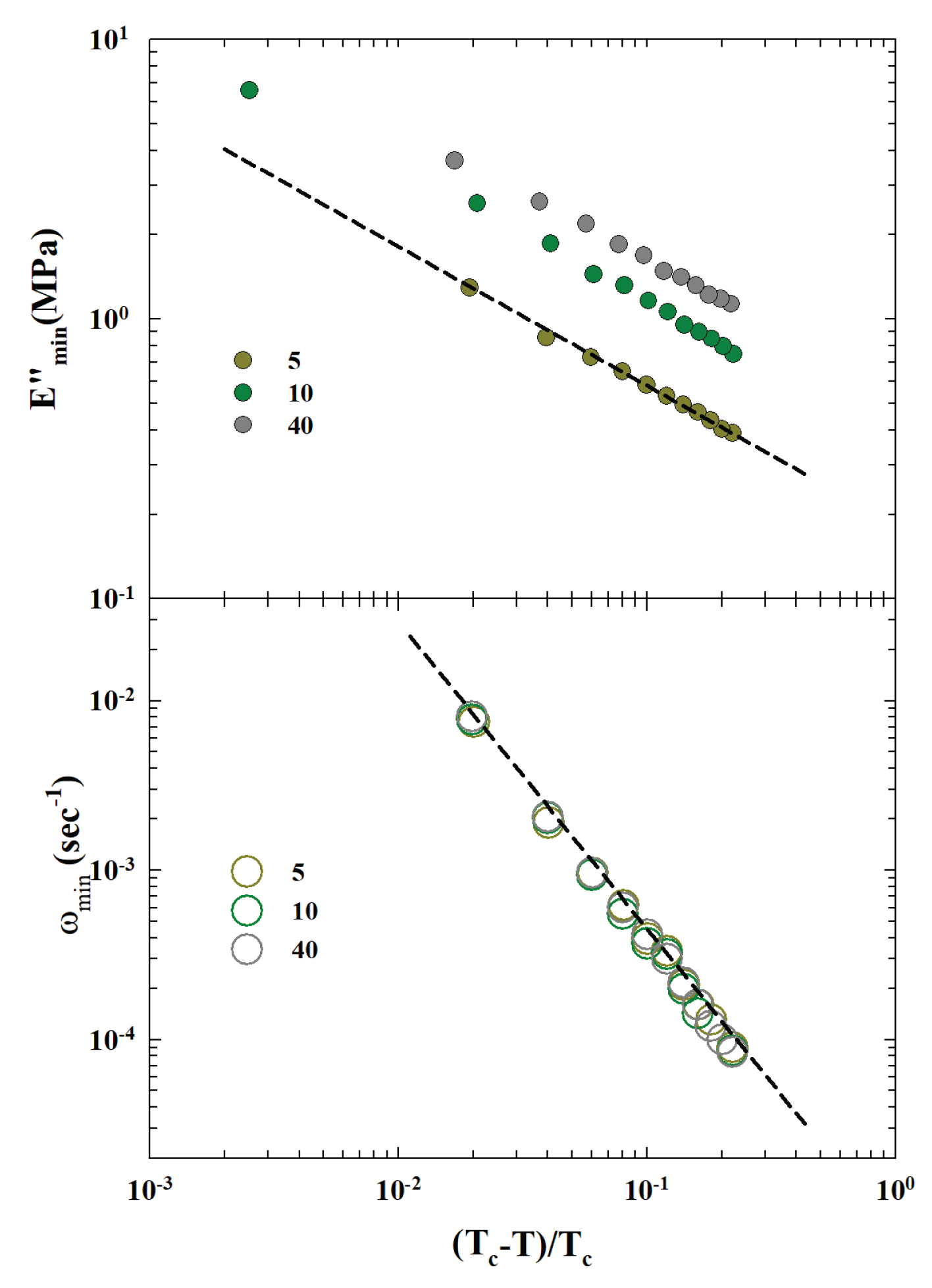
As previously proposed, being the MCT based on precise scaling laws (and the corresponding exponent values) of the measured physical quantities, respect to the control parameter we used some of these in order to confirm the validity of such a hypothesis on the of the studied materials. Hence, by considering, we explore the thermal behavior of the obtained and according to the corresponding MCT forms and .
Using the values 248 K (very close to the evaluated ) for the transition temperature, , we can check the power laws for the two relevant parameters and . The corresponding data behaviors, for , are proposed versus as a log-log plot in the Figure 8. As can be observed the two MTC scaling laws (for - bottom and - top) are well verified for that critical temperature. Both these obtained exponents are consistent with the MCT predictions on approaching ; in particular, we have that the exponent , whereas the predicted MCT value is .
This MCT scaling of and represents thus a new and important information on the dynamical properties of the studied SBR-CNT rubbers showing us what happens to their kinetic glass transition. In addition, this is a confirmation on the validity of the MCT approach not only for the analysis of the viscoelasticity parameters for the SBR-CNT rubbers in the region of the KGT, but in our opinion, also constitutes the proof that this theory represents a solid basis for dealing adequately with the complexity of the time temperature superposition process.
4. Concluding Remarks
By using the MCT model, developed for viscoelastic relaxation processes, we have verified the TTS validity instead of the best known and most used approach based on the Williams-Landel-Ferry equation (WLF) [16]. The main reason to operate by means of this fundamental model of statistical physics developed to clarify the basic and general phenomenon of the dynamic arrest (or glass transitions) by means of the scaling concepts typical of the universal critical transition [32] is that we can explore the chemical-physics processes underlying the TTS.
The studied system is Styrene-Butadiene rubbers (SBR) filled with Carbon Nanotubes (CNT) and Carbon Block (CB) whose elastic moduli have been evaluated at different concentrations and temperatures in the region of the sol-gel transtion.
In this frame, we have considered (it is usually done through the WLF) the measured frequency-dependent isotherms of the shear moduli . The starting idea is that the susceptibility spectra of the relaxing system are characterized by an evolution with maxima and minima. For the MCT description of the viscoelasticity the observed minima in loss moduli must scale according to the relation versus . In addition, MCT gives an interpolation form (equivalent to the main MCT form for correlators in the time regime) with which and can be evaluated [26]. Through the fitting of our experimental isotherms, with this form, it was possible for us to evaluate both and , together with the MCT exponents a and b.
Therefore, it was possible to operate the TTS by means of a multiplicative data shift of the obtained values of and . After which we considered a background contribution () in the resulting master curves which, subtracted, has evidenced for all the curves a precise frequency scaling () identical to the one previously suggested by the analysis of dielectric data [20]. In addition, these values have singular dependence with the filler (CNT) concentration, thus suggesting some dynamic effect due to the interaction between them and the SBR rubber.
Finally, considering this last fact, we studied the evolution in temperature of the obtained quantities from the fitting of the loss modulus isotherms. We first evaluated the evolution of the exponents a and b observing that also these quantities, especially b, show a significant dependence on the amount of the CNT. In particular, a grows with continuity, for all the studied C, up to a certain temperature ( K) after which they tend to saturate towards a constant value. The exponent b instead shows (at about this temperatures) a marked discontinuity for , whereas for and 1 its growth is moderate and continuous.
Much more significant for the dynamics of the system are the evolutions with T of both and . By means of an Arrhenius plot of the respective data it can be clearly seen that, while those of the two lowest concentrations, have over the entire studied T-range, a super-Arrhenius behavior; the others, show instead, by reducing T, a crossover on purely Arrhenius, around a certain temperature . In agreement with recent experimental observations, theoretical models of statistical physics and the MCT in its extended version, this is the evidence of the fragile to strong dynamic crossover characteristic of a kinetic glass transition, that just occurs near [13].
In conclusion, this result is the most significant, using MCT, to treat TTS of system response functions. In fact, it demonstrates that an interaction between the carbon nanotubes and the polymeric macromolecules of the rubber generates significant effects on the thermodynamics of the entire mixture. Specifically, it manages to change the temperature of its glass transition, bringing it to higher temperatures than that of the basic constituent (the pure SBR).
Result, this last one, confirmed by the MCT scaling behavior of and as a function of and the relative "critical" scaling as and are well verified for the critical temperature K; and the full consistence of the obtained exponents with the MCT predictions: in fact is , whereas the MCT predicted a value is .
Author Contributions
All authors contributed equally.
Data Availability Statement
The data that support the findings of this study are available from the corresponding author upon reasonable request.
Acknowledgments
The DM work was supported by the European Project H2020 A-LEAF - 732840.
References
- Kauzmann, W. The nature of the glassy state and the behavior of liquids at low temperatures. Chem. Rev. 1848, 43, 219–256. [Google Scholar] [CrossRef]
- Debenedetti, P. G. Metastable Liquids: Concepts and Principles; Princeton University Press: Princeton, 1996. [Google Scholar]
- Angell, C.A. Relaxation in liquids, polymers and plastic crystalsâ”strong/fragile patterns and problems. J. Non-Cryst. Solids 1991, 131-133, 13–31. [Google Scholar] [CrossRef]
- Stillinger, F.H. Supercooled liquids, glass transitions, and the Kauzmann paradox. J. Chem. Phys. 1988, 88, 7818. [Google Scholar] [CrossRef]
- Flory, P. Principles of Polymer Chemistry; Cornell University Press: Ithaca, 1953. [Google Scholar]
- Doi, M.; Edwards, S. F. Theory of Polymer Dynamics; Clarendon: Oxford, 1986. [Google Scholar]
- de Gennes, P.G. Scaling Concepts in Polymer Physics; Cornell University Press: Ithaca, 1979. [Google Scholar]
- Adam, G.; Gibbs, J.H. On the Temperature Dependence of Cooperative Relaxation Properties in Glass-Forming Liquids. J. Chem. Phys. 1965, 43, 139â–146. [Google Scholar] [CrossRef]
- Götze, W. Complex Dynamics of Glass-Forming Liquids A Mode-Coupling Theory; Oxford Univ. Press: Oxford, 2009. [Google Scholar]
- Dyre, J.C. The glass transition and elastic models of glass-forming liquids. Rev. Mod. Pys 2006, 78, 953–972. [Google Scholar] [CrossRef]
- Stillinger, F.H.; Debenedetti, P.G. Energy landscape diversity and supercooled liquid properties. J. Chem. Phys. 2002, 116, 3353. [Google Scholar] [CrossRef]
- Liao, A.; Parrinello, M. Escaping free-energy minima. Proc. Natl Acad. Sci. USA 2002, 99, 12562–12566. [Google Scholar] [CrossRef] [PubMed]
- Mallamace, F.; Branca, C.; Cosaro, C.; Leone, N.; Spooren, J.; Chen, S.-H.; Stanley, H.E. Transport properties of glass-forming liquids suggest that dynamic crossover temperature is as important as the glass transition temperature. Proc. Natl Acad. Sci. USA 2010, 28, 22457–22462. [Google Scholar] [CrossRef] [PubMed]
- Emri, I. Rheology of Solid Polymers. Rheol. Rev. 2005, 2005, 49. [Google Scholar]
- Ferry, J. D. Viscoelastic Properties of Polymers, 3rd ed.; John Wiley and Sons: New York, 1980. [Google Scholar]
- Williams, M.L.; Landel, R.F.; Ferry, J.D. The temperature dependence of relaxation mechanisms in amorphous polymers and other glass forming liquids. J. Am. Chem. Soc. 1955, 77, 3701–3707. [Google Scholar] [CrossRef]
- Vogel, H. Das temperaturabhangigkeitsgesetz der viskositat von flussigkeiten. Phys. Z. 1921, 22, 645. [Google Scholar]
- Fulcher, G.S. Analysis of recent measurements of the viscosity of glasses J. Am. Cer. Soc. 1925, 8, 339–355. [Google Scholar] [CrossRef]
- Tamman, S.; Hesse, W.Z. Die Abhangigkeit der Viscositat von der Temperatur bie unterkuhlten kussigkeiten Anorg. Allg. Chem. 1926, 156, 245. [Google Scholar] [CrossRef]
- Boye Olsen, N.; Christensen, T.; Dyre, J.C. Time-Temperature Superposition in Viscous Liquids. Phys. Rev. Lett. 2001, 86, 1721–1724. [Google Scholar]
- Barlow, A. J.; Lamb, J.; Matheson, A. J. Viscous behaviour of supercooled liquids. Proc. R. Soc. London A 1967, 298, 481. [Google Scholar]
- Montrose, C.J.; Litovitz, T.A. Structural Relaxation Dynamics in Liquids. J. Acoust. Soc. Am. 1970, 47, 1250. [Google Scholar] [CrossRef]
- Garcia, G.; Salzano de Luna, M.; Mensitieri, G.; Escobar, M.; Mansille, M.; Baldanza, A. Carbon nanotubes networking in Styrene-butadiene rubber: a dynamic mechanical and dielectric spectroscopic study. Macromol. Mater. Eng. 2023; 306, 2200514. [Google Scholar]
- Chong, S.H. Connections of activated hopping processes with the breakdown of the Stokes-Einstein relation and with aspects of dynamical heterogeneities. Phys. Rev. E 2008, 78, 041501. [Google Scholar] [CrossRef]
- Chong, S.H.; Chen, S.H.; Mallamace, F. A possible scenario for the fragile-to-strong dynamic crossover predicted by the extended mode-coupling theory for glass transition. J. Phys. Cond. Matter 2009, 21, 504101. [Google Scholar] [CrossRef]
- Bengtzelius, U.; Götze, W.; Sjolander, A. Dynamics of supercooled liquids and the glass transition. J. Phys. C 1984, 17, 5915–5934. [Google Scholar] [CrossRef]
- Essam, J. Percolation theory. Rep. Prog. Phys. 1980, 43, 833–912. [Google Scholar] [CrossRef]
- de Gennes, P.G. On a relation between percolation theory and the elasticity of gels. J.Phys.(France)Lett 1976, 37, L1. [Google Scholar] [CrossRef]
- Efros A., L.; Shkolovskii, B. I. Critical Behaviour of Conductivity and Dielectric Constant near the Metal-Non-Metal Transition Threshold. Phys. Status Solidi B, 1976; 76, 475–485. [Google Scholar]
- Chong, S.H. Connections of activated hopping processes with the breakdown of the Stokes-Einstein relation and with aspects of dynamical heterogeneities. Phys. Rev. E 2008, 78, 041501. [Google Scholar] [CrossRef] [PubMed]
- Chong, S.H.; Chen, S.H.; Mallamace, F. A possible scenario for the fragile-to-strong dynamic crossover predicted by the extended mode-coupling theory for glass transition. J. Phys. Cond. Matter 2009, 21, 504101. [Google Scholar]
- Stanley, H. E. Introduction to Phase Transition and Critical Phenomena; Oxford University Press: Oxford, 1971. [Google Scholar]
Figure 1.
The tensile moduli, storage () and loss (), measured by means of the DMA in Styrene Butadiene Rubber filled with Carbon Nanotubes (CNT) at the concentration (phrCNT, phr-parts per hundred rubber)), in the temperature range K, for frequencies () in the range to 100 () left side. In the top of right side, the data fitting of the loss moduli according to the MCT viscoelasticity model, whereas at the bottom are reported the corresponding MCT time-temperature superposition (TTS) curves. All the data are represented in a log-log plot. Data from [23].
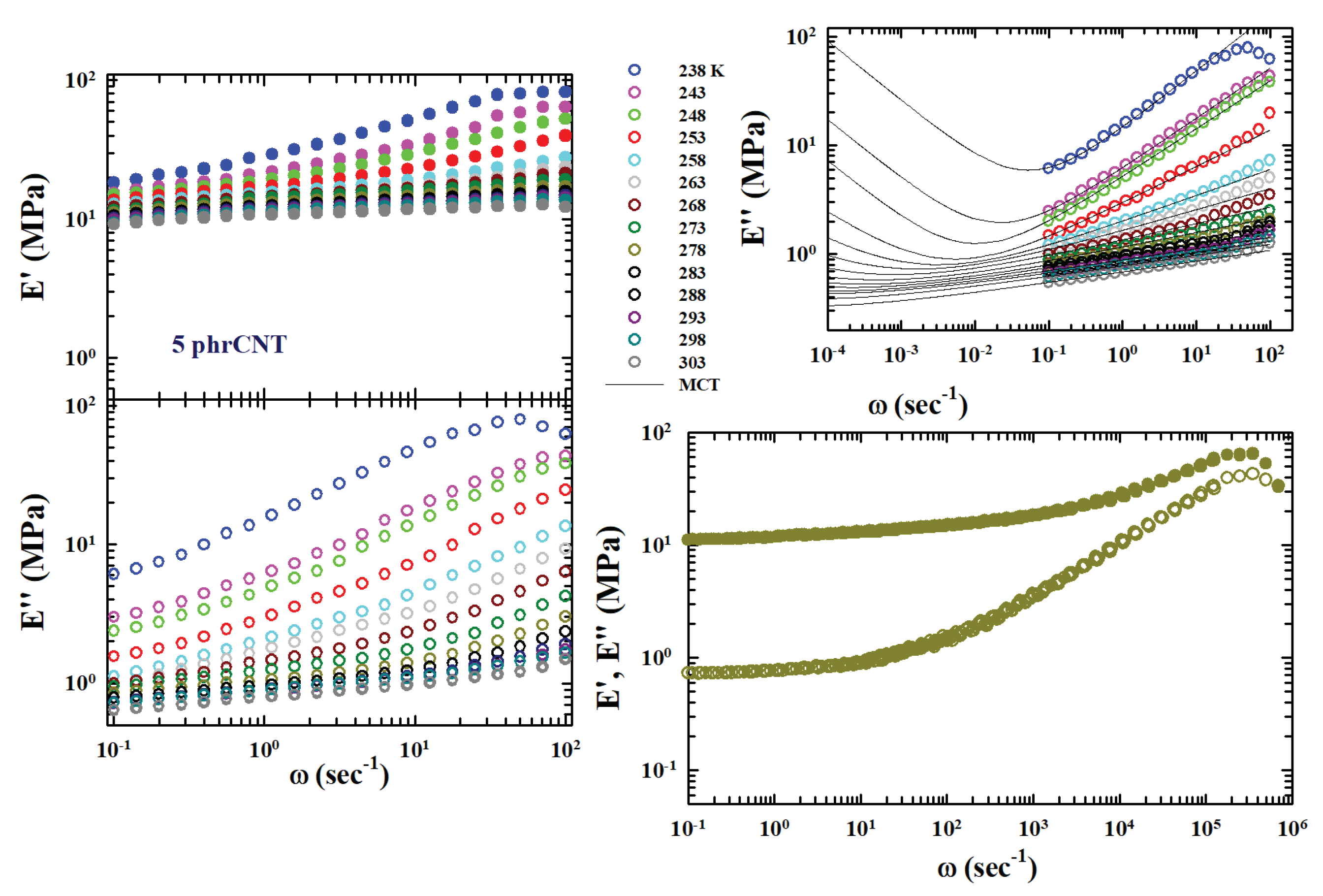
Figure 2.
The MCT time-temperature superposition (TTS) curves for storage () and loss () moduli, for the all the studied phrCNT concentrations and 40, in a log-log plot.
Figure 2.
The MCT time-temperature superposition (TTS) curves for storage () and loss () moduli, for the all the studied phrCNT concentrations and 40, in a log-log plot.
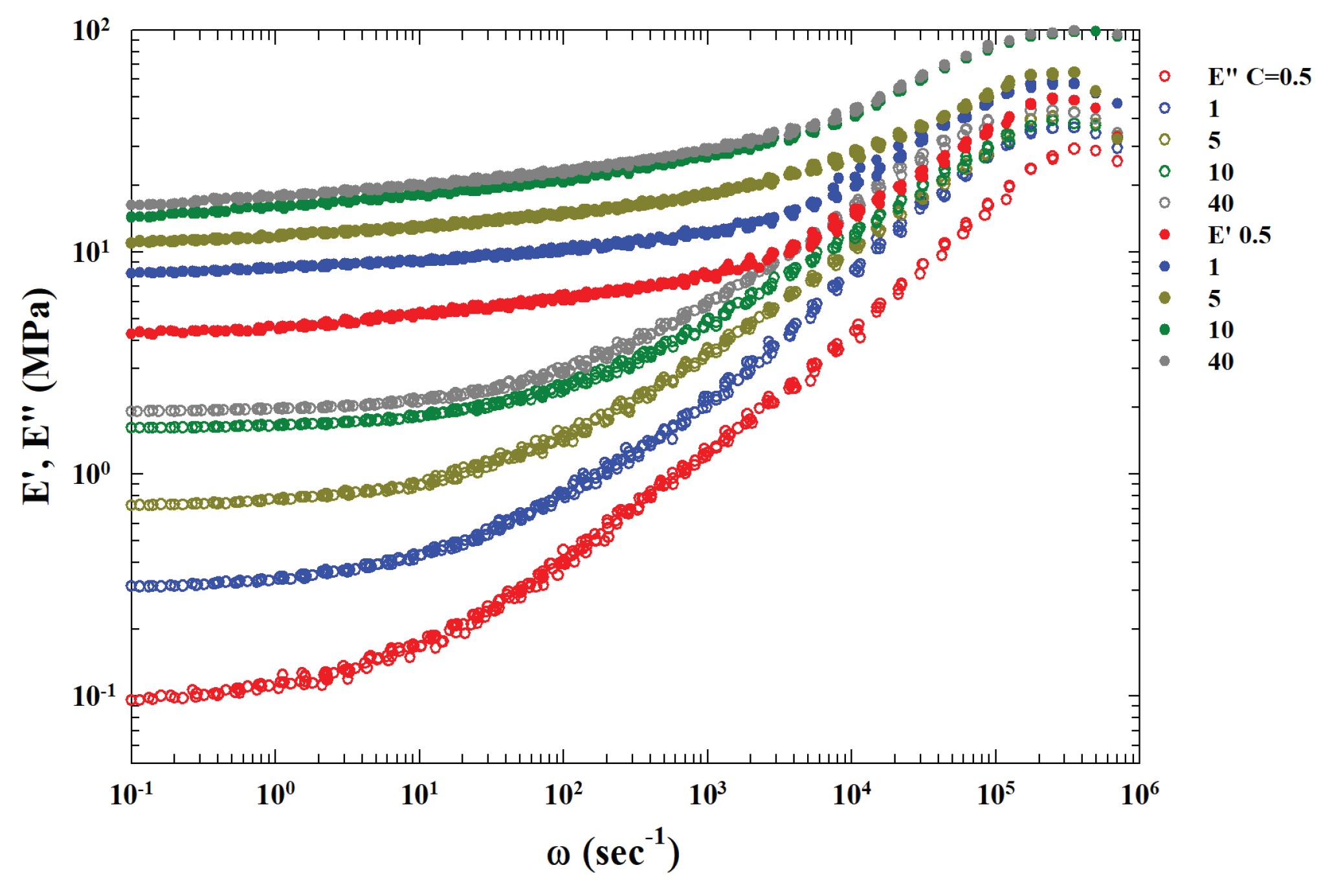
Figure 3.
The TTS master curves after the subtraction of an extra background . This, by assuming that is the asymptotic value of the moduli at low frequencies. The obtained and are thus reported as fully and open symbols, respectively. Of particular interest is in this log-log representation the resulting loss moduli behavior: a power-law behavior (the straight lines) with a slope of about . In the figure inset is proposed the contribution as a function of the concentration C, and the dotted line, as discussed in the text, is a data fitting in terms of a logistic function.
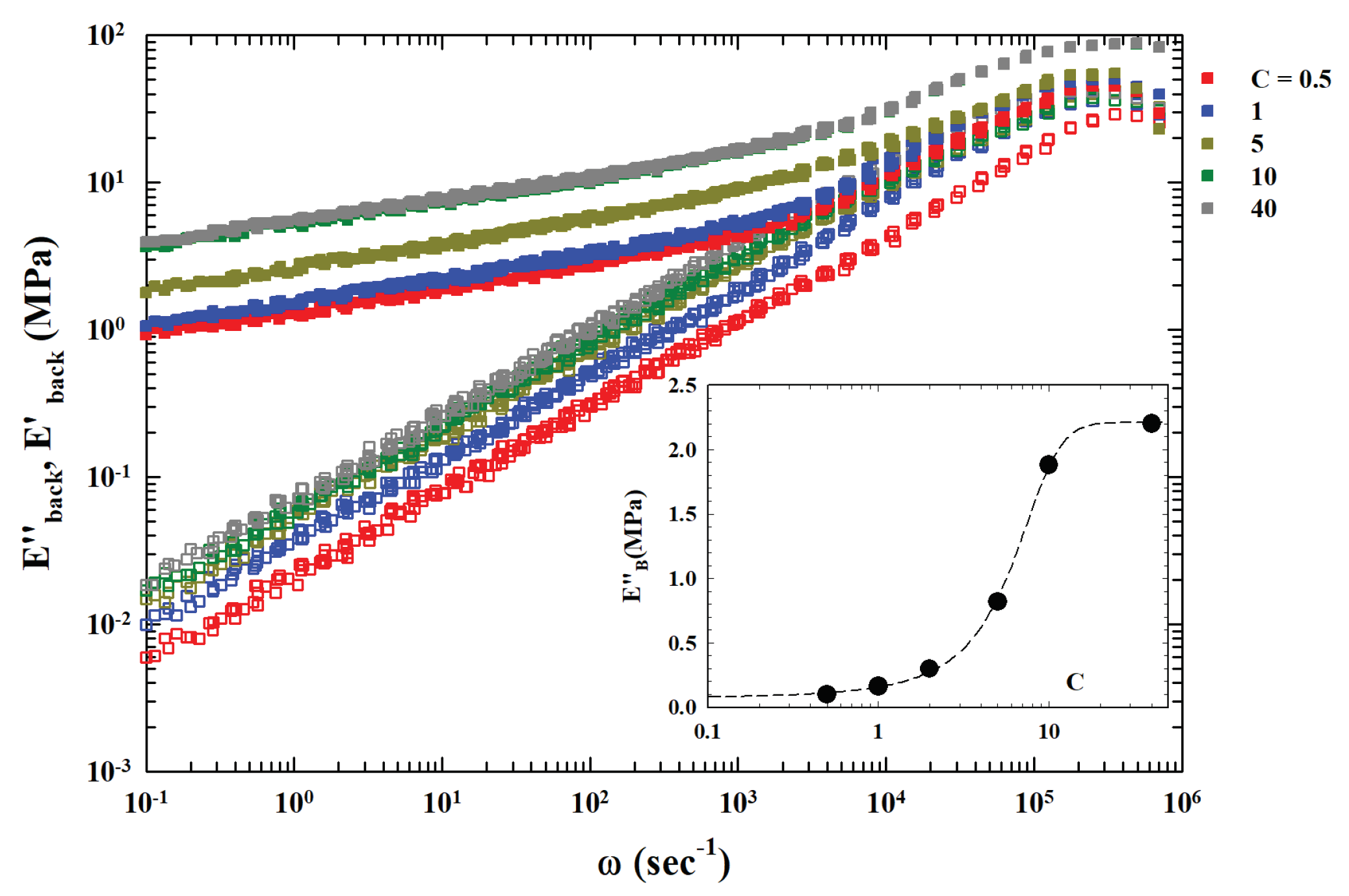
Figure 4.
The TTF master curves representing the , superimposed as , according to a simple procedure that considers the values.
Figure 4.
The TTF master curves representing the , superimposed as , according to a simple procedure that considers the values.
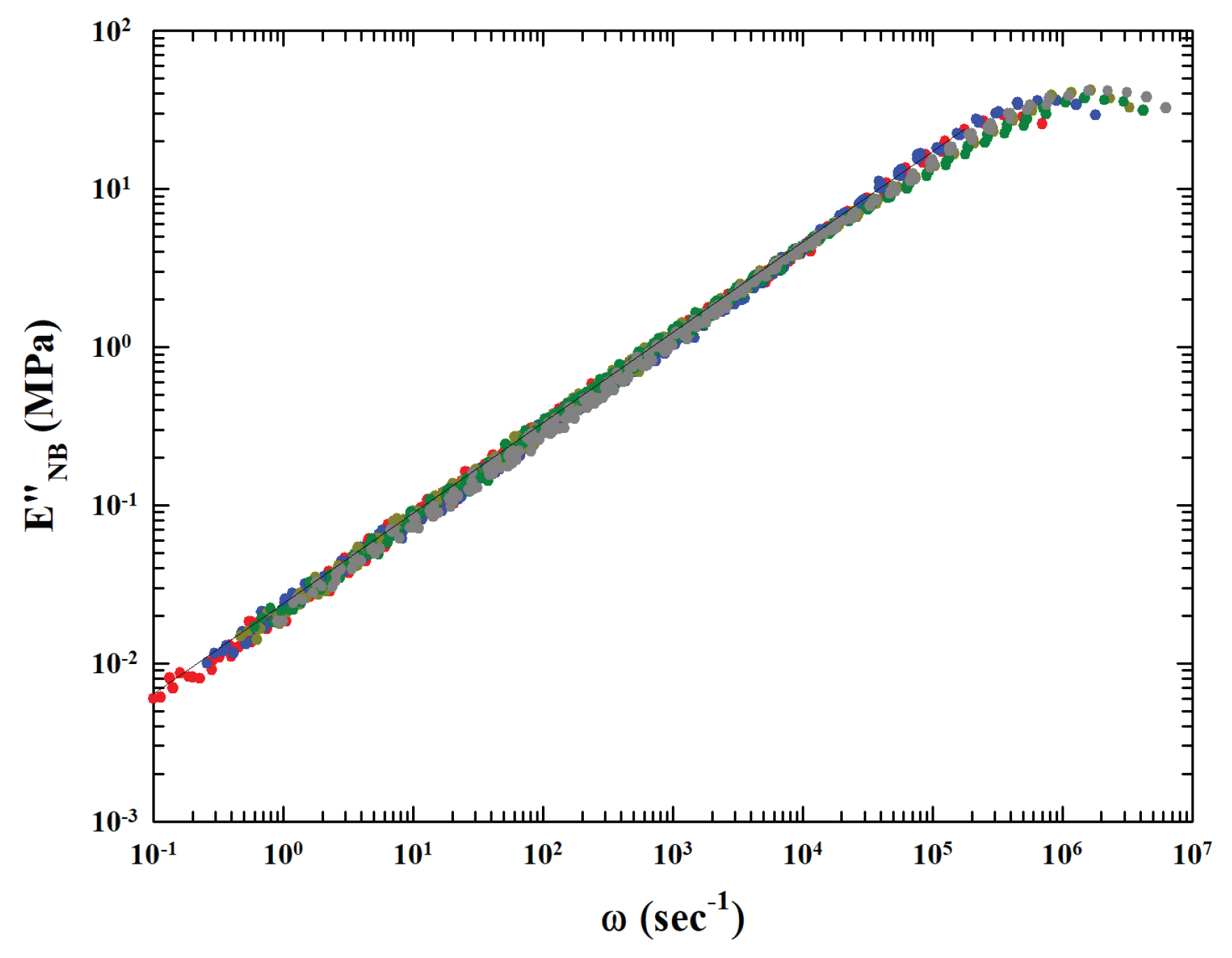
Figure 5.
The Figure report (at increasing value of C in a clockwise way) the storage and loss moduli, along with the loss angle tangent (), measured at the two extreme temperatures 238 and 303 K, for the several different used concentrations (). From the illustrated data it is easily observable that at the highest temperature (303) and for , and are essentially constant for all the explored range.
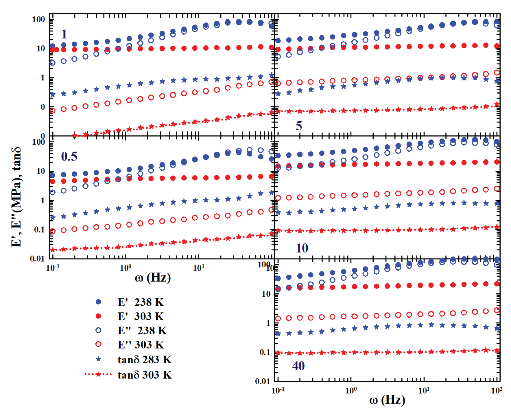
Figure 6.
The dependence of the MCT exponents a and b obtained from the loss moduli data fitting (the lines are a guide for the eyes). While a grows continuously (almost exponential), for all the concentrations, up to a certain temperature ( K) after which they tend to saturate towards a constant value, b instead shows (around the same T), for a marked discontinuity.
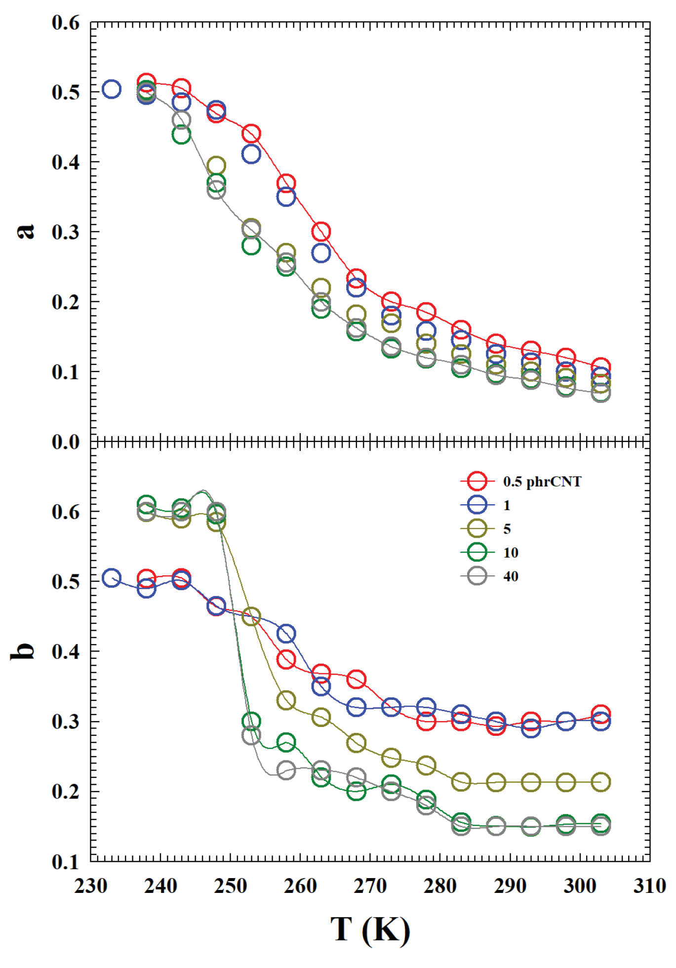
Figure 7.
The Arrhenius representation of and , showing a different a different dependence. While at the lower phrCNT ( and 1) the and are nearly equal and exhibit a super-Arrhenius behavior (dotted curve), for a SFDC crossover can be observed for both at K (dashed line). In this last case , unlike , show a strong C dependence.
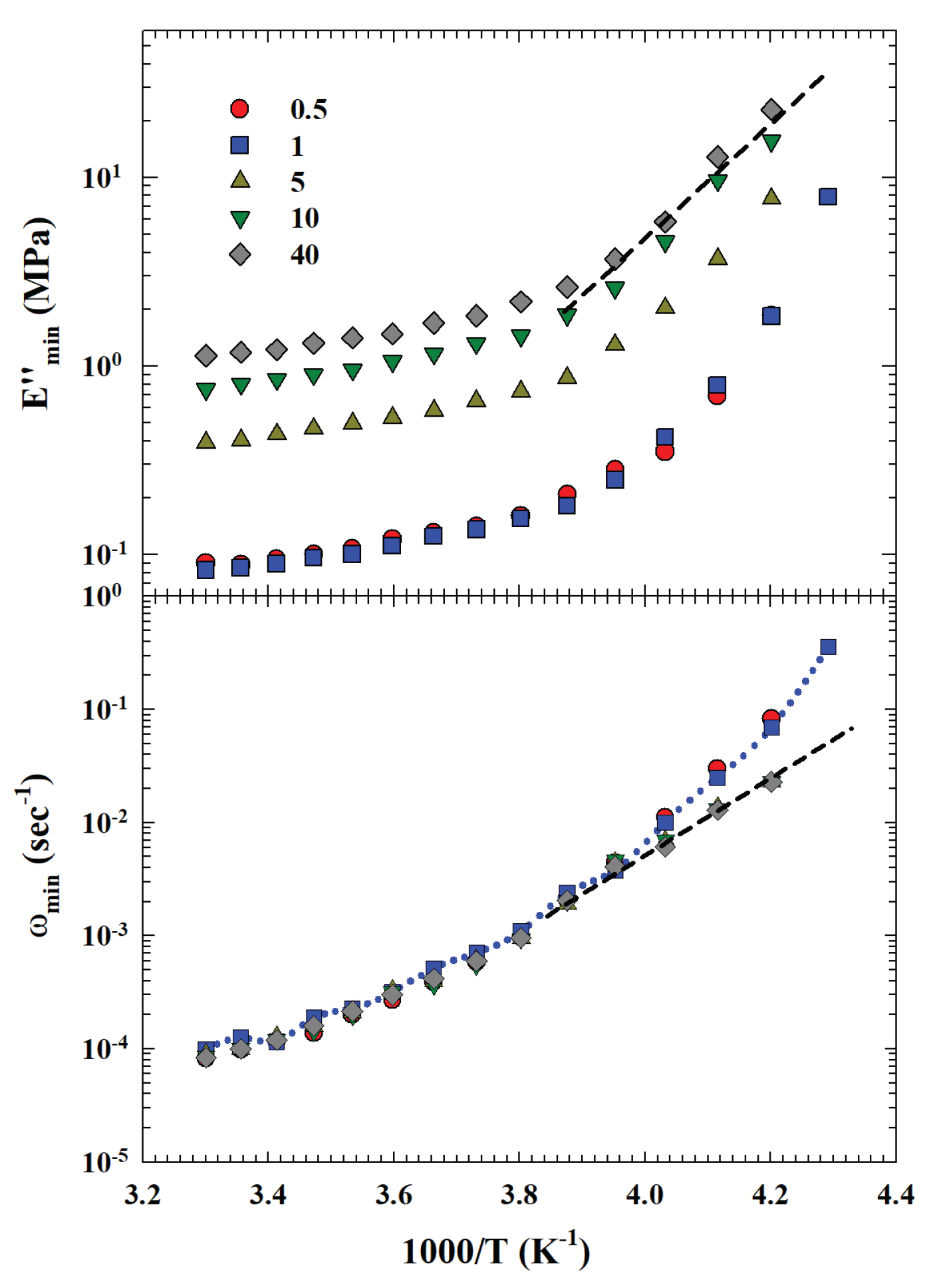
Figure 8.
The critical temperature behavior of and . The value of the MTC critical temperature is for both quantities 248 K. The plotted dashed straight lines give the corresponding critical index: for and for .
Figure 8.
The critical temperature behavior of and . The value of the MTC critical temperature is for both quantities 248 K. The plotted dashed straight lines give the corresponding critical index: for and for .
Disclaimer/Publisher’s Note: The statements, opinions and data contained in all publications are solely those of the individual author(s) and contributor(s) and not of MDPI and/or the editor(s). MDPI and/or the editor(s) disclaim responsibility for any injury to people or property resulting from any ideas, methods, instructions or products referred to in the content. |
© 2024 by the authors. Licensee MDPI, Basel, Switzerland. This article is an open access article distributed under the terms and conditions of the Creative Commons Attribution (CC BY) license (http://creativecommons.org/licenses/by/4.0/).
Copyright: This open access article is published under a Creative Commons CC BY 4.0 license, which permit the free download, distribution, and reuse, provided that the author and preprint are cited in any reuse.


