Multivariate Hydrologycal Modelling based on Long Short Term Memory Networks for Water Level Forecasting.

In this work, a novel approach is presented for the multivariate prediction of hydrological variables, employing a specialized type of recurrent neural network (RNN) known as the long-term memory network (LSTM).The central objective is to develop a flood prediction model using data collected from two hydrological stations situated along the Atrato River in the Choc´o Department, Colombia. The interconnected variables of water level, water flow, and water precipitation are analyzed in this model to enhance flood prediction accuracy. The LSTM model, integrated into an RNN structure, is designed to capture the complex dynamics and cross-correlations inherent in these hydrological variables. Validation involves a comparison with linear and nonlinear Nonlinear AutoRegressive with eXogenous input (NARX) models, considering factors such as estimation error and computational time. Additionally, the study conducts further analysis for water level prediction under two scenarios: utilizing only outflow and inflow measurements or predicting outflow alongside measuring inflow, with the objective of utilizing the proposed approach as a flood early warning system. † This article is a revised and expanded version of a paper entitled Multivariable NARX based Neural Networks Models for Short-term Water Level Forecasting, which was presented at International Conference on Time Series and Forecasting (ITISE-2023), Gran Canaria, Spain, 12th-14th July, 2023.

Keywords:

Subject: Engineering - Electrical and Electronic Engineering

1. Introduction

Precision in hydrological variable modeling is paramount for effective flood forecasting and the sustainable management of water resources. This importance is highlighted by the complex relationships between climatic elements, river discharge dynamics, and local environmental characteristics. Leveraging advanced techniques like Long Short Term Memory (LSTM) networks, adept at discerning intricate temporal patterns within multivariate datasets, this research seeks to elevate the accuracy and dependability of water level predictions. These strides are essential for fortifying resilience against hydrological risks and optimizing resource allocation in regions susceptible to such challenges in [1]. Two primary techniques are commonly employed for this purpose: white-box algorithms, rooted in mathematical modeling, and black-box algorithms, utilizing nonlinear neural network techniques based on Machine Learning models. Among neural network techniques, Long Short-Term Memory (LSTM) recurrent neural networks are notable, capable of analyzing sequences of input data and generating predictions [2]. As a type of recurrent neural network (RNN), LSTM can capture both long-term and short-term dependencies among sequential data time units [3]. The significance of LSTM neural networks in predicting future time instants is emphasized in [4], in which an LSTM model is suggested for Forecasting floods, Using the river discharge and daily precipitation as input data. examining features influencing model performance. In [5], The efficacy of multiple models, comprising LSTM, Convolutional Neural Network LSTM (CNN-LSTM), Convolutional LSTM (ConvLSTM), and Spatiotemporal Attention LSTM (STA-LSTM), is evaluated for flood prediction. Additionally, [6] presents the development of an urban flood forecasting and warning system in South Korea’s main flood risk area. This system utilizes a rainfall-runoff model and a deep learning model incorporating LSTM recurrent neural networks to mitigate potential damage.

In [7], proposes a precipitation forecasting model by extrapolating Cloud Top Brightness Temperature (CTBT) using advanced Deep Neural Networks, and applying the predicted CTBT to an efficient precipitation retrieval algorithm to obtain Quantitative Short-Term (0-6 h) Precipitation Forecasting. To achieve such tasks, we propose Long Short-Term Memory (LSTM) and Precipitation Estimation from Remotely Sensed Information using Artificial Neural Networks (PERSIANN), respectively, in [8], compares the performance of three deep and machine learning-based rainfall forecasting approaches, including a PSO-optimized hybrid support vector regression (PSO-SVR), a long-short term memory (LSTM), and a convolutional neural network (CNN). The approaches are used to develop 5- and 15-min forecast models of rainfall depth based on datasets from Niavaran station, Tehran, Iran, in[9], the main objective was to compare the accuracy of four data-driven techniques: linear regression (LR), multilayer perceptron (MLP), support vector machine (SVM) and long-term memory network (LSTM) in daily flow forecasting. For this purpose, three scenarios were defined based on 26-year historical series of precipitation and flow rates of the Kentucky River basin, located in eastern Kentucky (USA).In [10] this paper, we attempt to provide a new method to perform forecasting using the long-term memory deep learning model (LSTM), which targets the field of time series data.In addition, In the study conducted.In [11], a flood forecasting model aimed at predicting future flood occurrences is designed and assessed. This is achieved by creating a hybrid deep learning algorithm known as ConvLSTM, which combines the predictive capabilities of Convolutional Neural Network (CNN) and Long Short-Term Memory Network (LSTM).

In [12] the study concentrates on using a combined deep learning method, specifically a CNN-LSTM model, to predict both water level and water quality simultaneously. This hybrid architecture incorporates convolutional neural networks (CNN) for extracting spatial features and long short-term memory (LSTM) networks to capture temporal dependencies within the data, in [13]this paper focuses on integrating a hybrid CNN-LSTM deep learning model with a boundary-corrected maximal overlap discrete wavelet transform for multiscale lake water level forecasting in [14] this article focuses on water level forecasting using a spatiotemporal attention-based long short-term memory (LSTM) network, in [15]this paper introduces a hybrid method for basin water level prediction, utilizing Long Short-Term Memory (LSTM) networks and precipitation data.

Several studies within flood forecasting and monitoring have explored different Artificial Neural Network (ANN) techniques.[16], assessed the bias correction of real-time precipitation data to improve hydrological models, employing ANN bias correction for enhanced real-time flood forecasting.[17] focused on developing five distinct ANN models for flood forecasting and conducted a comparative analysis of their performance. In another study by [18], a multilayer perceptron was utilized to construct a flood prediction model with flow as input-output variables, demonstrating its effectiveness through comprehensive experiments.[19] designed a flood monitoring system integrating flow and water level sensors, employing a two-class neural network to predict flood status from database-stored data.[20] utilized a Convolutional Neural Network (CNN) to forecast time series variables like water level in a flood model, showcasing the versatility of CNNs beyond their conventional use in two-dimensional image classification with transfer learning.

This study explores and evaluates the implementation of a multivariate LSTM model based on recurrent neural networks (RNN) for predicting water levels in the Atrato River, located in the Chocó department, Colombia, over both short and long-term periods. The research utilizes data from two hydrological stations on the Atrato River, monitored by the Institute of Hydrology, Meteorology, and Environmental Studies (IDEAM). These data include measurements of flow rate, precipitation, and water level sampled every 12 hours over a span of 789 days.

In this study, a multivariate Long Short-Term Memory (LSTM) model with 4 inputs and 2 outputs is employed. This model is trained to predict water levels at each station, incorporating inputs such as water level, water flow, and precipitation. It considers the intrinsic dynamics and correlations within the hydrological process. The model’s performance is evaluated using metrics like root mean square error (RMSE) and the Nash-Sutcliffe efficiency coefficient (NSE), which compare the model’s predictions to actual data.

The primary contribution of this research involves formulation of a multivariate LSTM model based on recurrent neural networks for short and long-term water level prediction. It is noteworthy that LSTM networks have the ability to "remember" relevant information from the sequence and retain it over multiple time steps, resembling the way our brain analyzes sequences. For instance, when reading a buyer’s review to make decisions, the LSTM network mimics our approach by focusing on words deemed relevant and discarding non-essential information.

The structure of the work is outlined as follows: it begins with the presentation of the theoretical framework, introducing hydrological variables and the Nonlinear AutoRegressive with eXogenous input (NARX) model for their dynamic approximation. Following that, the experimental setup and detailed estimation results are provided, concluding with final observations and comments.

2. Theoretical Framework

2.1. LSTM (Long Short-Term Memory) Network

An LSTM is a special functional block of recurrent neural networks (RNN) with a short-term to long-term memory[21]. It is an evolution of RNNs and helps to solve the evanescent gradient problem, where during training the gradients of the weights become smaller and smaller and thus the network stops storing useful information[22]. LSTM cells have three types of gates - an input gate, a memory and forgetting gate, and an output gate - for storing memories of past experiences. Short-term memory is retained for a long time and network[23] behavior is encoded in the weights. LSTM networks are particularly well suited for making predictions based on time-series data, such as handwritten text recognition and speech recognition.

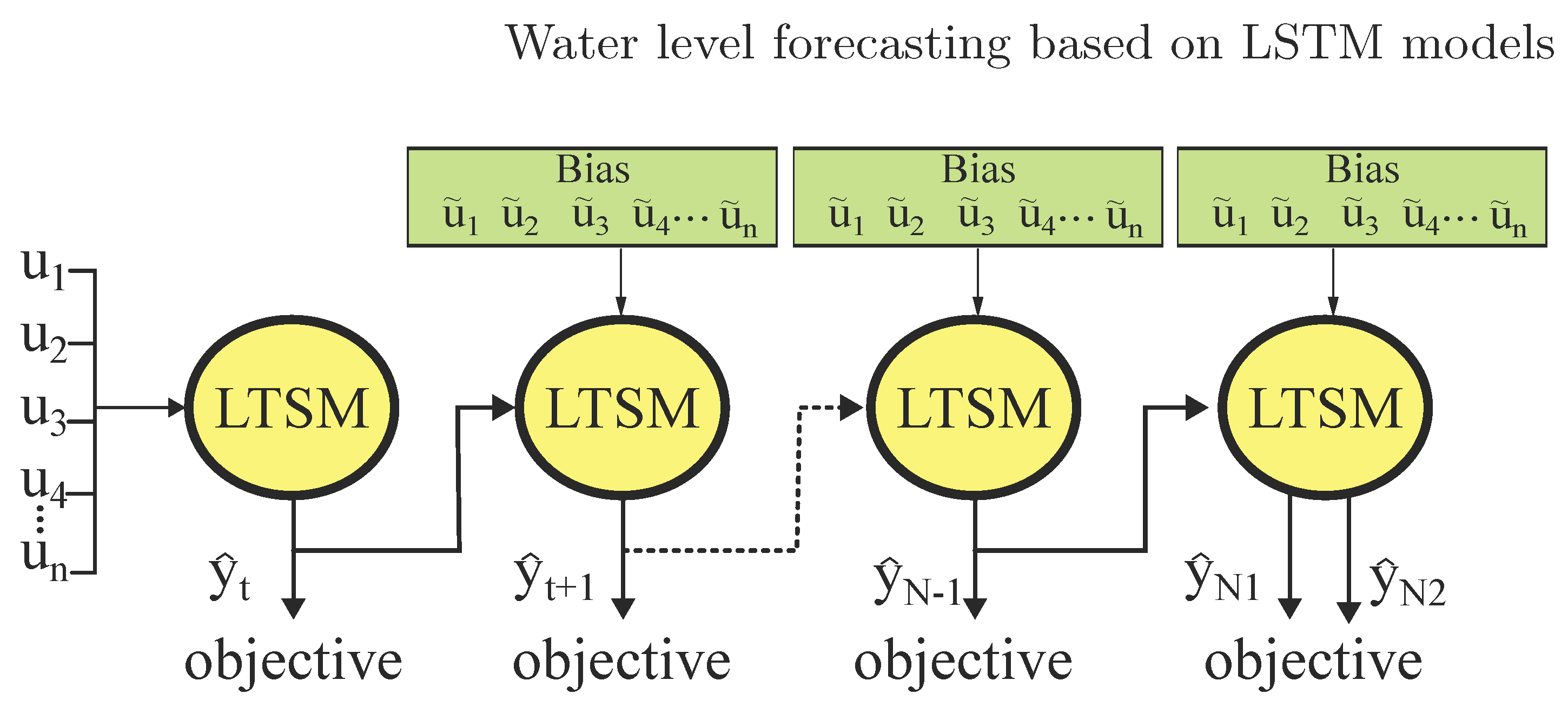
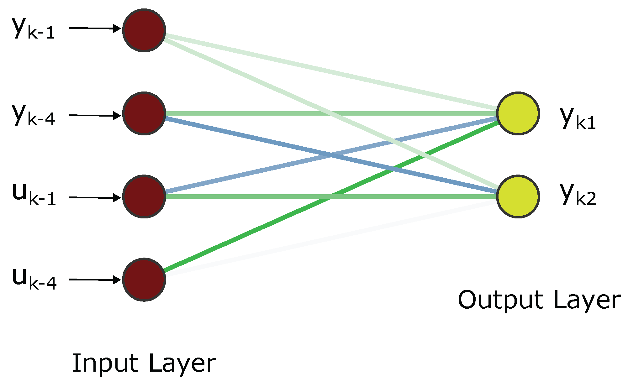
Furthermore, LSTM architecture has emerged to address these issues. Unlike traditional Recurrent Neural Networks (RNNs), where retaining past data for extended periods poses challenges, LSTM addresses this limitation effectively. With a total of six parameters and a four-gate structure, LSTM can manage both short-term and long-term memory effectively. for our multivariable model we employ the structure in Figure 1.

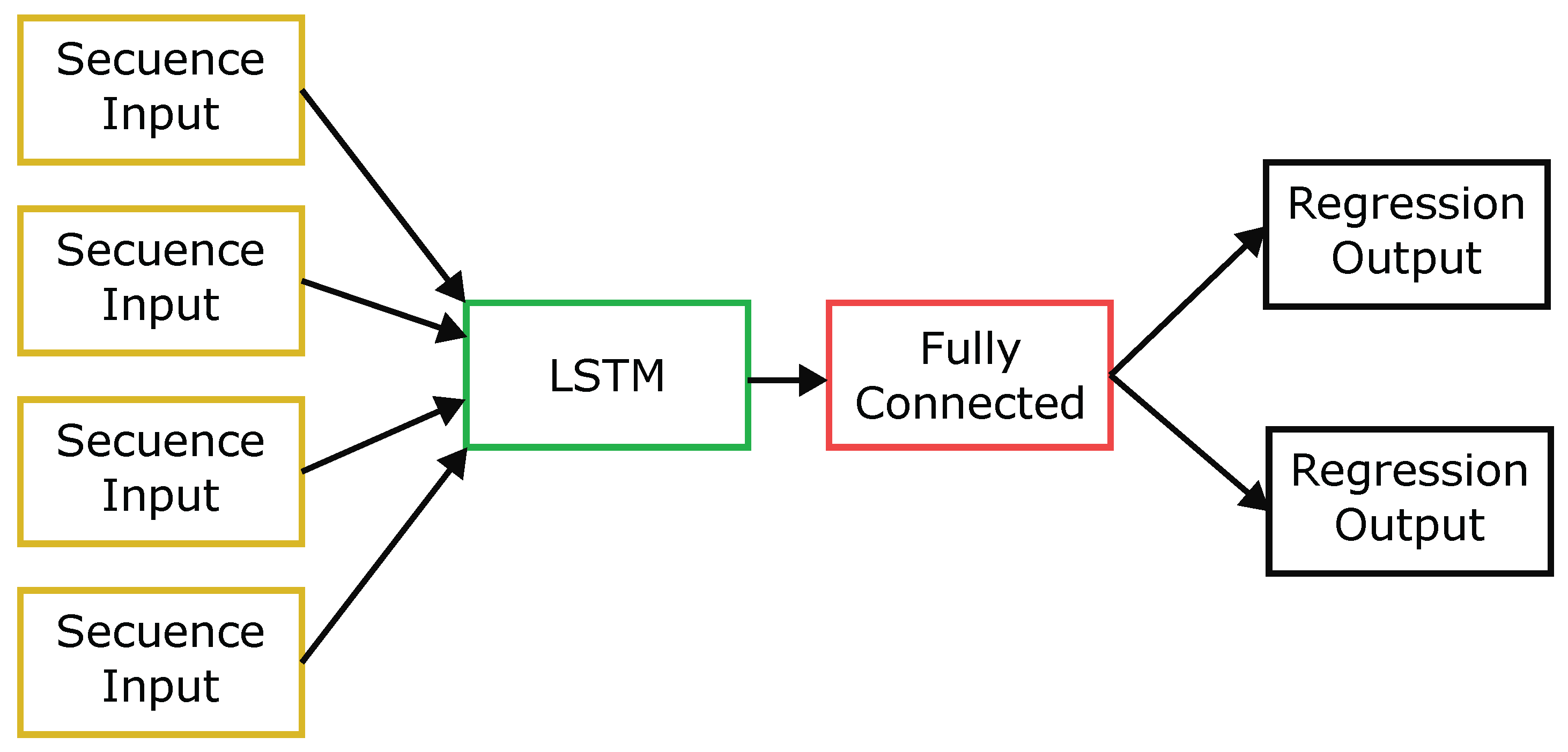
In Figure 2 the neural network starts with an input layer of sequences followed by an LSTM layer. The neural network ends with a fully connected layer and an output regression layer.

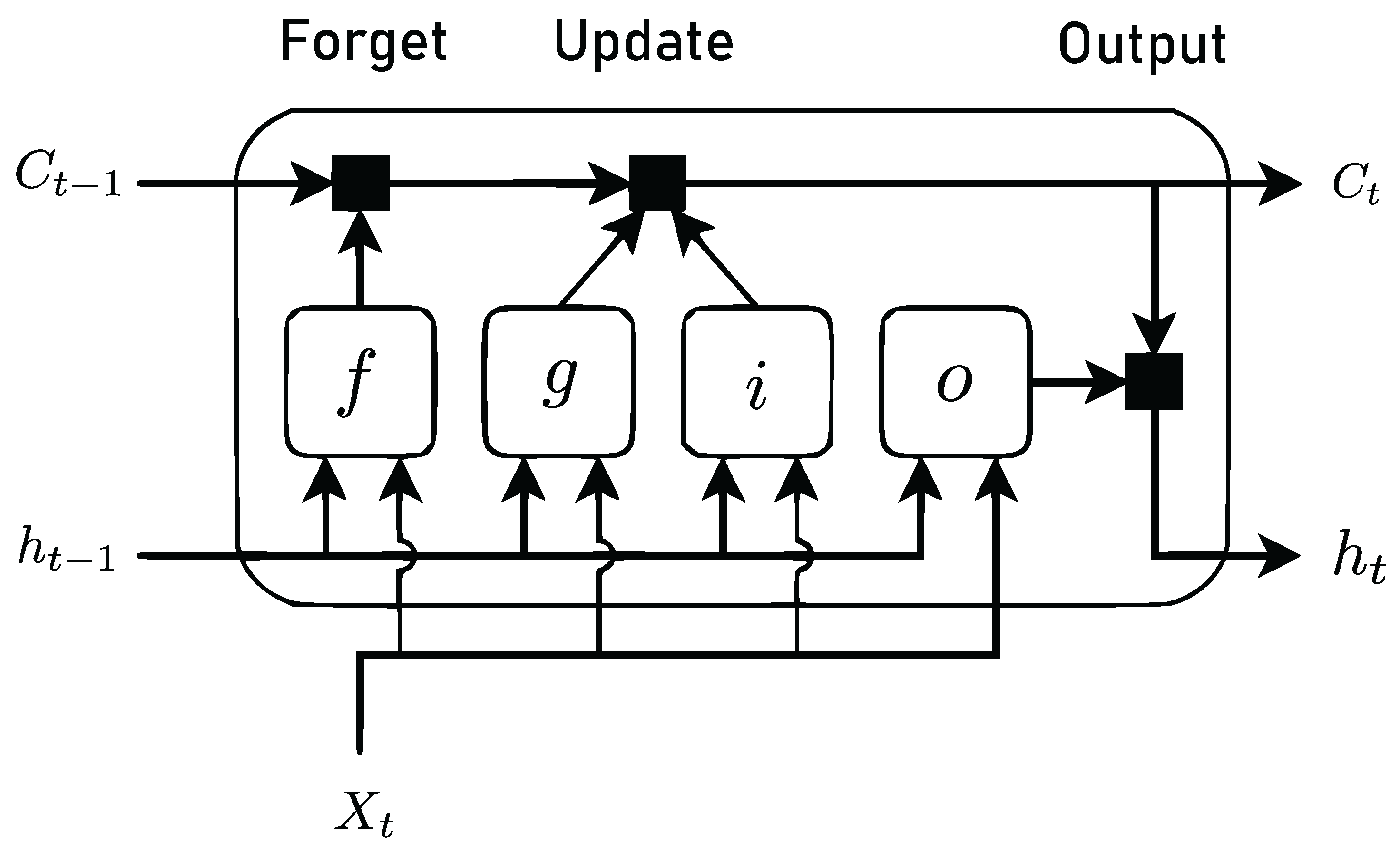
In Figure 3 the diagram shows how the gates forget, update and generate the cell and hidden states.These components control the state of the cell and the hidden state of the layer, among these are: entrance door (i), door of oblivion (f), Cell candidate (g), exit door (o).

The weights that can be learned from the LSTM layer are input weights W (InputWeights), recurrence weights R (RecurrentWeights) and bias b (Bias). The matrices W, R and b are the combination of input weights, cycle weights and offsets for each component, respectively. This layer connects matrices according to the following equation (1):

\begin{matrix} W = [\begin{matrix} W_{i} \\ W_{f} \\ W_{g} \\ W_{0} \end{matrix}], R = [\begin{matrix} R_{i} \\ R_{f} \\ R_{g} \\ R_{0} \end{matrix}], b = [\begin{matrix} b_{i} \\ b_{f} \\ b_{g} \\ b_{o} \end{matrix}] \end{matrix}

(1)

,where i, f, g and o determine the entry gate, forgetting gate, cell candidate and exit gate, respectively.

The cell state at time unit t is given by (2)

\begin{matrix} C_{t} = f_{t} ⊙ C_{t - 1} + i_{t} ⊙ g_{t}, \end{matrix}

(2)

,where ⊙ determines the Hadamard product (element-level vector multiplication).

The hidden state at time unit t is given by (3)

\begin{matrix} h_{t} = o_{t} ⊙ σ_{c} + C_{t}, \end{matrix}

(3)

,where

σ_{c}

determines the state activation function. By default, the lstmLayer function uses the hyperbolic tangent function (tanh) to calculate the state activation function.

The equations of the components in time unit t are described below.

in (4),we describe the gateway equation entrance door, in (5) oblivion door , in (6) cell candidate, in (7) open door.

\begin{matrix} i_{t} = σ_{g} (W_{i} X_{t} + R_{i} h_{t - 1} + b_{i}) \end{matrix}

(4)

\begin{matrix} f_{t} = σ_{g} (W_{f} X_{t} + R_{f} h_{t - 1} + b_{f}) \end{matrix}

(5)

\begin{matrix} g_{t} = σ_{c} (W_{g} X_{t} + R_{g} h_{t - 1} + b_{g}) \end{matrix}

(6)

\begin{matrix} o_{t} = σ_{g} (W_{o} X_{t} + R_{o} h_{t - 1} + b_{o}) \end{matrix}

(7)

2.2. Hydrological Variables

To forecast water levels based on river dynamics, two hydrological stations are strategically positioned along the river. To address the correlation among all system variables and their respective nonlinearities, a suggested nonlinear dynamical model is introduced. Equation (8) illustrates the inputs and outputs of the proposed model.

\begin{matrix} y [k] = [\begin{matrix} y_{L_{1}} [k] \\ y_{L_{2}} [k] \end{matrix}], u [k] = [\begin{matrix} u_{F_{1}} [k] \\ u_{P T_{1}} [k] \\ u_{F_{2}} [k] \\ u_{P T_{2}} [k] \end{matrix}] \end{matrix}

(8)

Therefore,

y_{L_{1}} [k]

y_{L_{2}} [k]

respond to the 2 level outputs of the model ,

u_{F_{1}} [k]

u_{F_{2}} [k]

u_{P T_{1}} [k]

u_{P T_{2}} [k]

set the 4 inputs of the LSTM recurrent neural network system..

The dynamics of hydrological variables are modeled by employing a recurrent neural network (RNN), a type of artificial neural network designed for sequential or time series data, utilizing Long Short-Term Memory (LSTM) architecture, as expressed below:

\begin{matrix} y [k] = f (y [k - 1], \dots, y [k - n], u [k - 1], \dots, u [k - n]) + η [k] \end{matrix}

(9)

being n the order of the LSTM model and

f (.)

the nonlinear function, and

η [k]

the additive noise at time instant k.

2.3. Narx Based Neural Network Structure

NARX model (equation (9)) with inputs selected as

u [k - j]

and

y [k - j]

, representing a 4-th order model (

n = 4

) based on an in [24] analysis. This choice, supported by the research, this entails 24 inputs and 2 outputs, accounting for the variables. in the equation (8).

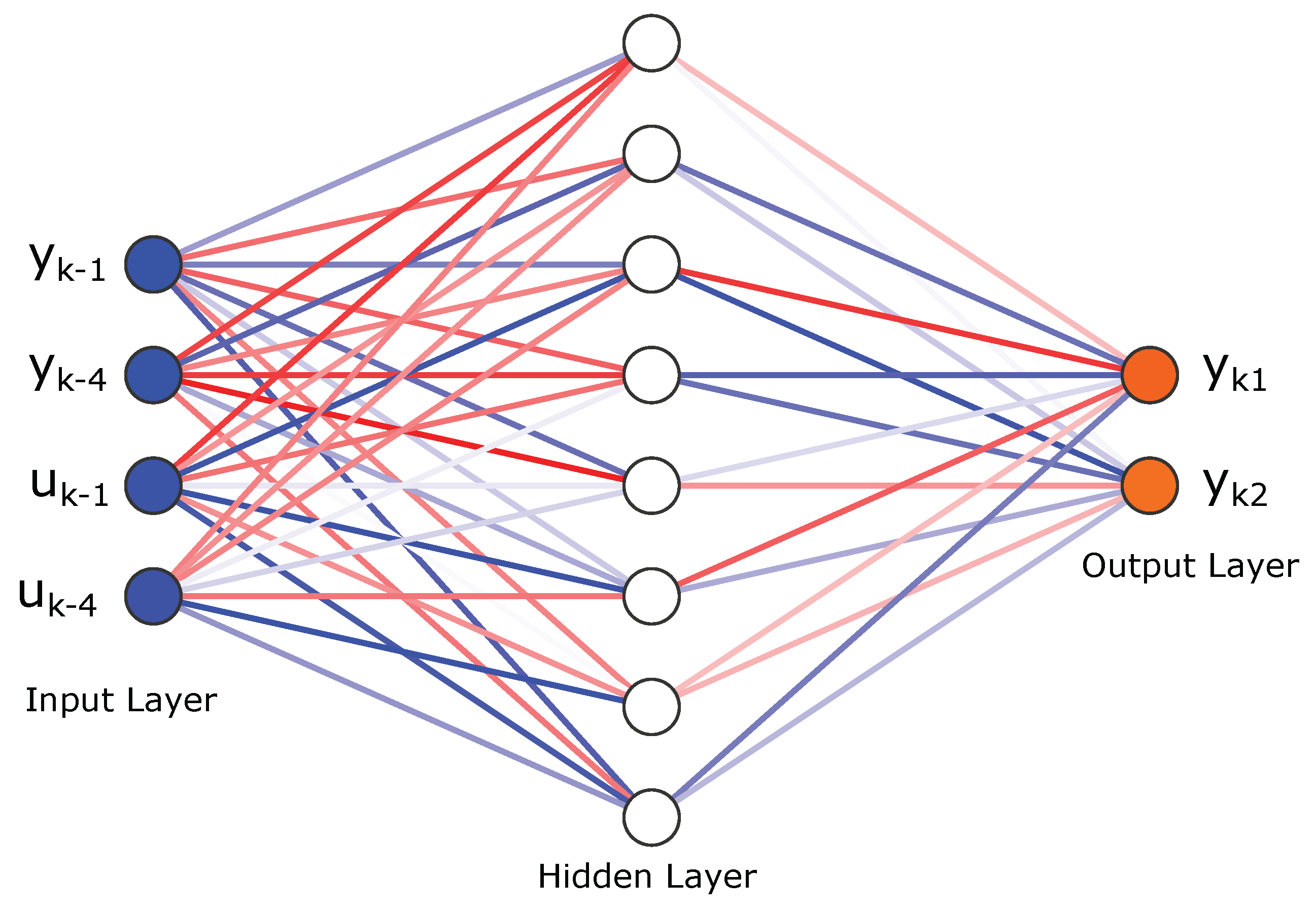
To approximate the nonlinear function in equation (9), a neural network structure

f^{*} (.)

is used as an approximation for the nonlinear function

f (.)

, depicted in Figure 4.

NARX model defined as follows:

\begin{matrix} y [k] = f^{*} (y [k - 1], \dots, y [k - n], u [k - 1], \dots, u [k - n]) + η [k] \end{matrix}

(10)

A linear AutoRegressive with eXogenous input (ARX) structure can be derived by omitting the hidden layer, as illustrated in the following Figure 5

The ARX model can be defined as follows:

\begin{matrix} y [k] = - \sum_{j = 1}^{4} a_{j} y [k - j] + \sum_{j = 1}^{4} b_{j} u [k - j] \end{matrix}

(11)

The equation involves parameters

A_{j}

and

B_{j}

for the model matrix, where y represents outputs, u signifies inputs, and

j = 1

denotes the system order. The variable p indicates the system order, while

e [k]

denotes noise, with m being the system’s number of outputs and inputs (

y [k] \in R^{m \times 1}

and

u [k] \in R^{m \times 1}

2.4. Hydrologycal Stations

The Atrato River, situated in Colombia, ranks as the third most navigable river in the country, following the Magdalena River and the Cauca River. Originating in the Cerro del Plateado, it traverses the Chocó department, serving as a vital means of transportation in the region and forming a natural border between Chocó and Antioquia. With a length of 750 km and a width fluctuating between 150 to 500 m, the river is a crucial component of the biogeographic Chocó, recognized for its remarkable biodiversity and considerable rainfall. Flowing into the Gulf of Urabá, it boasts 18 mouths forming the river delta and is acknowledged by the World Wildlife Fund as one of the world’s richest genetic banks.

Regarding meteorological data, the chosen information primarily encompasses flow rates, levels, and precipitation from two hydrological stations along the river. Each station provides measurements for these three variables, totaling 789 days of data sampling for each variable in both stations.

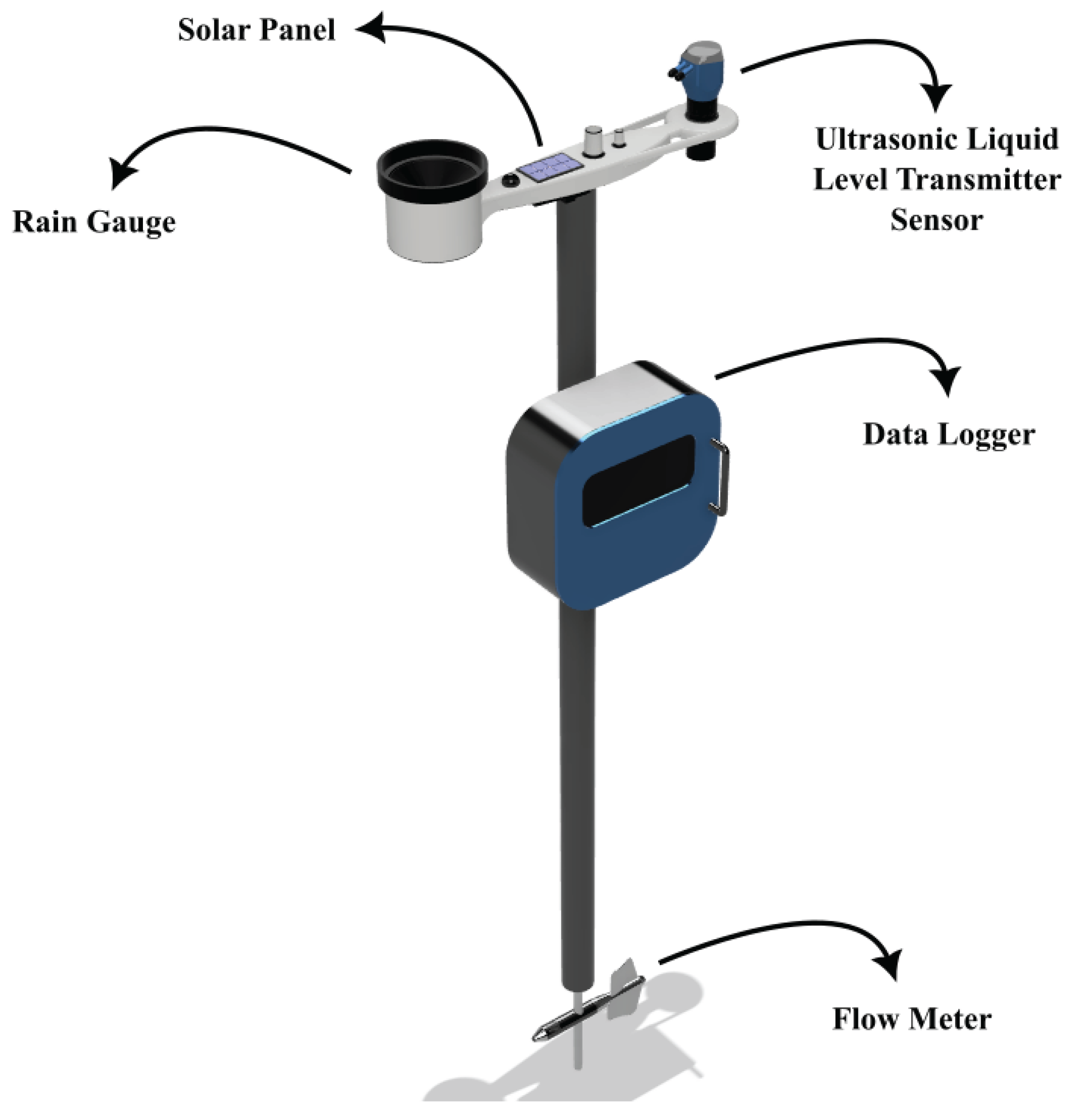
Figure 6 depicts the prototype station considered in the case study of this article, consisting of an ultrasonic level sensor, a water flow sensor, and a precipitation sensor.

Multiple measurement stations strategically placed along the river enable tracking variable dynamics at various locations, leading to the establishment of a multivariable coupled model due to the inherent interdependence of measured variables.Hydrological data from two stations, namely water flow and precipitation in the Atrato River, serve as input to the training model. Water level data from the two hydrological stations are used as the predicted output, resulting in a short- and long-term system with a training model structure comprising 24 inputs and 2 outputs for an order 4 system.

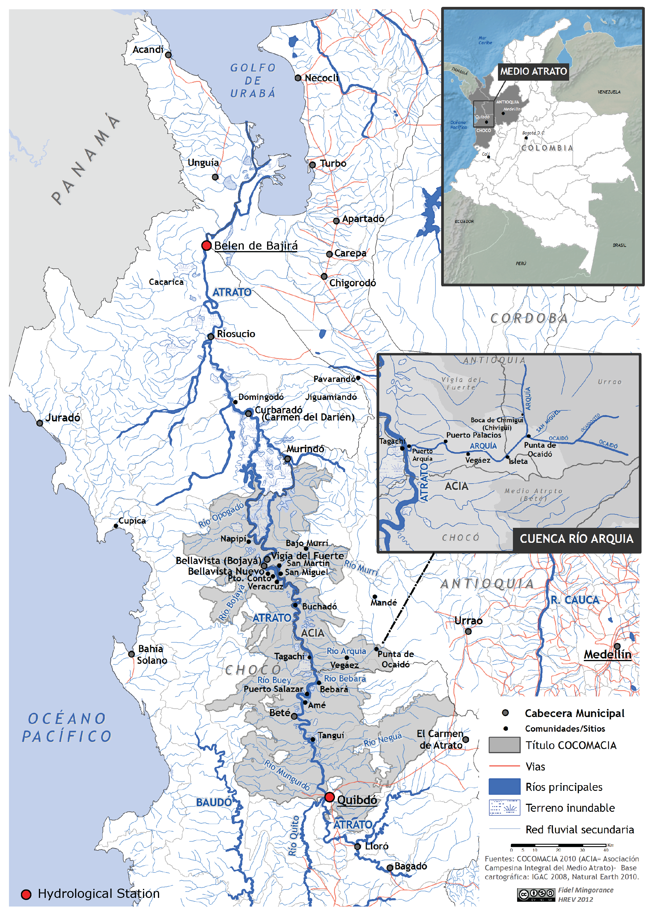
In Figure 7 shows the location of the hydrological stations and the exact place where the data collection of the proposed case study is carried out. Hydrological stations are located at Colombia, Department of Chocó .

2.5. Regression Metrics for the Estimation of the Quadratic Error

In this study, assessing prediction performance is crucial for gauging the model’s quality and optimizing efficiency. Two indicators are employed to evaluate the prediction performance of the outputs from the LSTM recurrent neural network model, further validating the proposed model against the non-linear NARX and linear ARX models. Regression metrics, including root mean square error (RMSE) and the Nash-Sutcliffe efficiency coefficient (NSE), are utilized to quantify the error in predictions.

The following are the mathematical formulas with which the error regression metrics[25] will be calculated.

\begin{matrix} \begin{matrix} R M S E = \sqrt{\frac{1}{n} \sum_{i = 1}^{n} {(y_{0_{i}} - y_{i})}^{2}} \end{matrix} \end{matrix}

(12)

\begin{matrix} \begin{matrix} N S E = 1 - \frac{\sum_{i = 1}^{n} {(y_{0_{i}} - y_{i})}^{2}}{\sum_{i = 1}^{n} (y_{0_{i}} - {\bar{y_{0})}}^{2}} \end{matrix} \end{matrix}

(13)

3. Results

3.1. Experimental Setup

To validate the proposed methodology, real-world data from two hydrological stations situated along the Atrato River in Colombia are utilized. The dataset comprises recorded variables such as water level, water flow, and precipitation. These actual data points serve as crucial inputs for testing the efficacy and accuracy of the developed model in predicting hydrological phenomena. The Atrato River, with a length of 750 km and a width varying between 150m and 500m, has depths ranging from 31m to

38 m

. The dataset covers 789 days, sampled every 12 hours, starting on January 1, 2021. The recurrent neural network LSTM model, designed for both short and long-term applications, is validated against a nonlinear NARX model and a linear ARX model.

In Table 1 are shown the geographical positions of the hydrological stations.

To validate the proposed approach, two analyses are conducted in this study. The first aspect involves comparing the short and long-term recurrent neural network (LSTM) approach for a 4th-order system. This validation includes a visual comparison of real and estimated signals using NARX and ARX methods, along with a quantitative evaluation based on root mean square error (RMSE) and the Nash-Sutcliffe efficiency coefficient (NSE). It is noteworthy that the long short-term memory (LSTM) recurrent neural network plays a pivotal role in deep learning, particularly in modeling sequences and temporal dependencies. In hydrology, LSTM is applied to predict river water levels, as implemented in this study. LSTM addresses the challenge of capturing short and long-term patterns in data, crucial for understanding the dynamics of hydrological variables over time. In this approach, LSTM is trained to forecast both short-term, considering immediate patterns, and long-term, considering dependencies across extensive sequences. The LSTM’s ability to retain relevant information over time makes it a valuable tool in modeling complex hydrological systems. The LSTM’s network structure comprises a hidden layer with 64 units, featuring the capability to remember previous states by introducing loops in the network diagram.The second aspect relates to a forecasting approach for future time steps based on predictions and measurements. It’s important to note that, for this analysis, 90% of the data sample is chosen to train the LSTM recurrent neural network (RNN), corresponding to 1417 out of 1578 total data points. This training is validated through a test, using the remaining 10%, equivalent to 158 data points from the total sample.

3.2. Estimation Results

This subsection showcases the outcomes of short- and long-term forecasting using the multivariate LSTM model for a system of order 4. Additionally, it examines the short-term response of the multivariate NARX and ARX models.

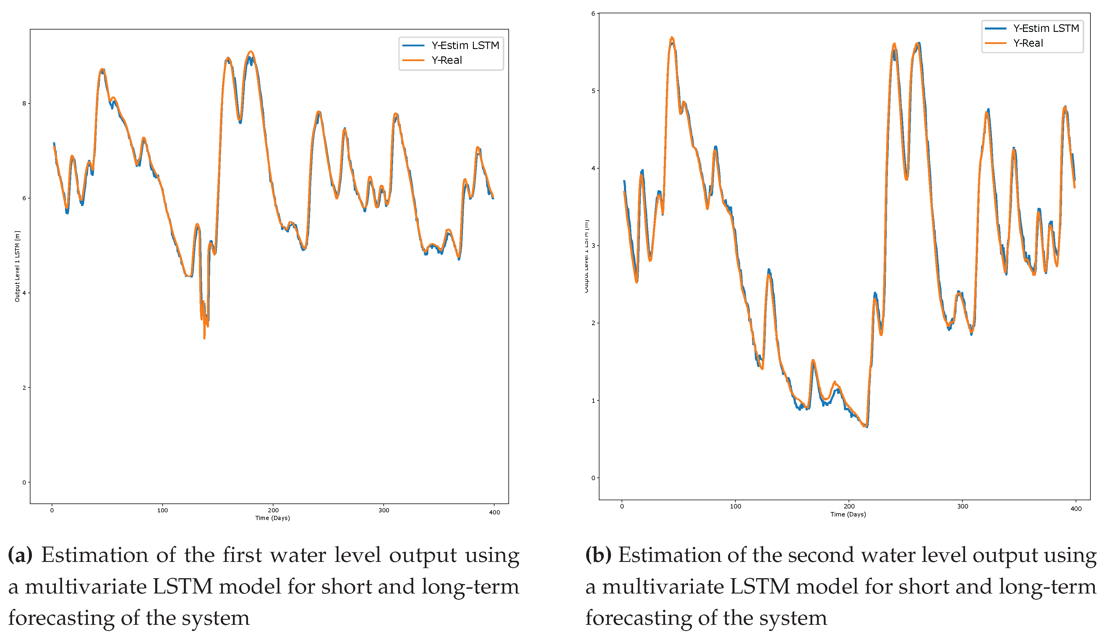
The outcomes of the LSTM method for both water level outputs are depicted in Figure 8. Specifically, Figure 8 displays the short-term estimation results for the first water level output, juxtaposed with the actual measurements. Similarly, Figure 8 exhibits the short-term forecasting outcomes for the second water level output, accompanied by the corresponding real measurements.

Figure 8a and Figure 8b demonstrate that the real measurements are effectively estimated through the utilization of the multivariate LSTM model.

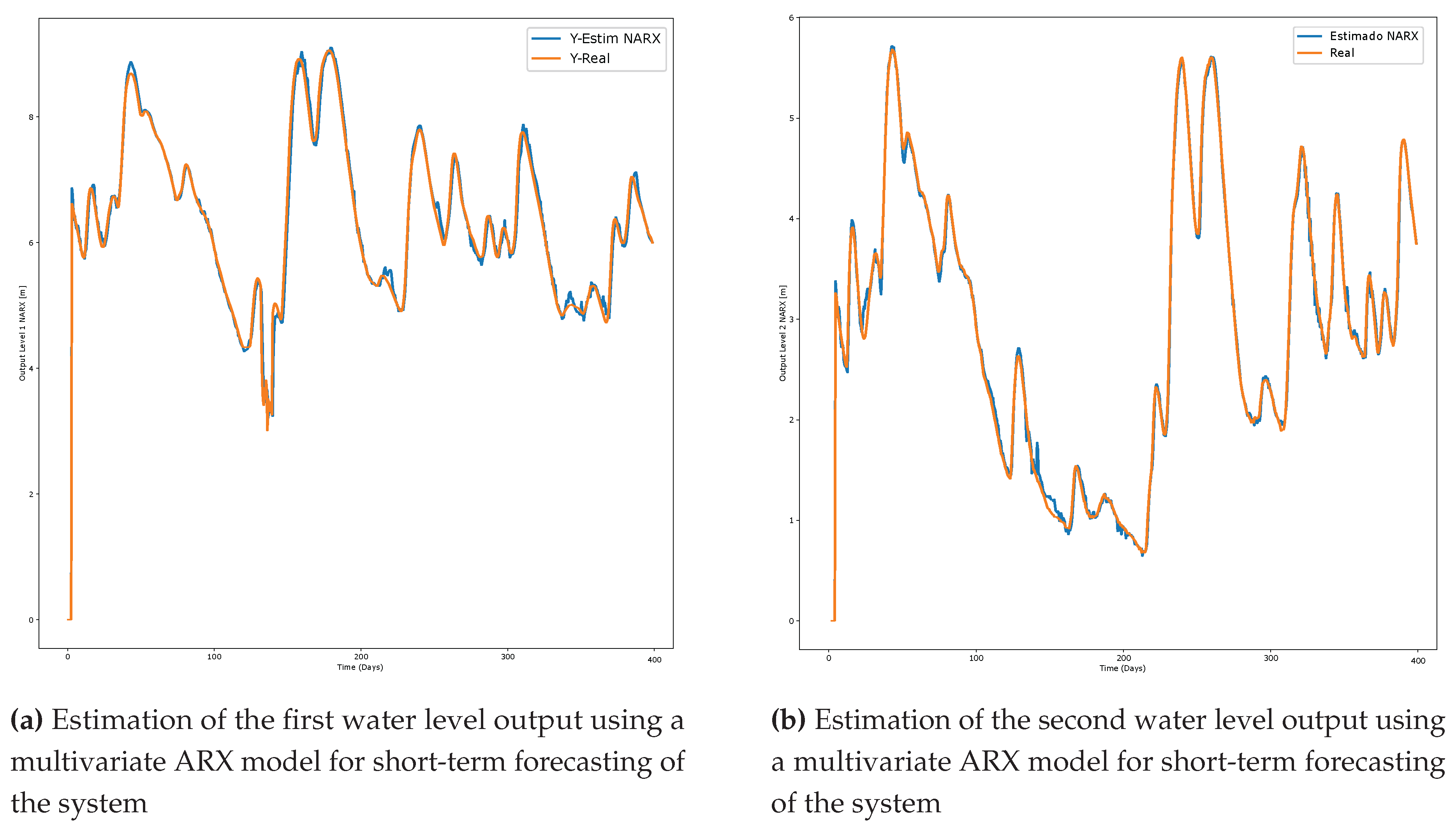
The outcomes of the multivariate NARX method for both water level outputs are presented in Figure 9, employing 64 nodes in the hidden layer, as specified in Table 3. Specifically, Figure 9 exhibits the short-term estimation of the first water level output, in comparison with the actual measurements. Additionally, Figure 9 illustrates the short-term water level forecasting for the second output, along with the corresponding real measurements.

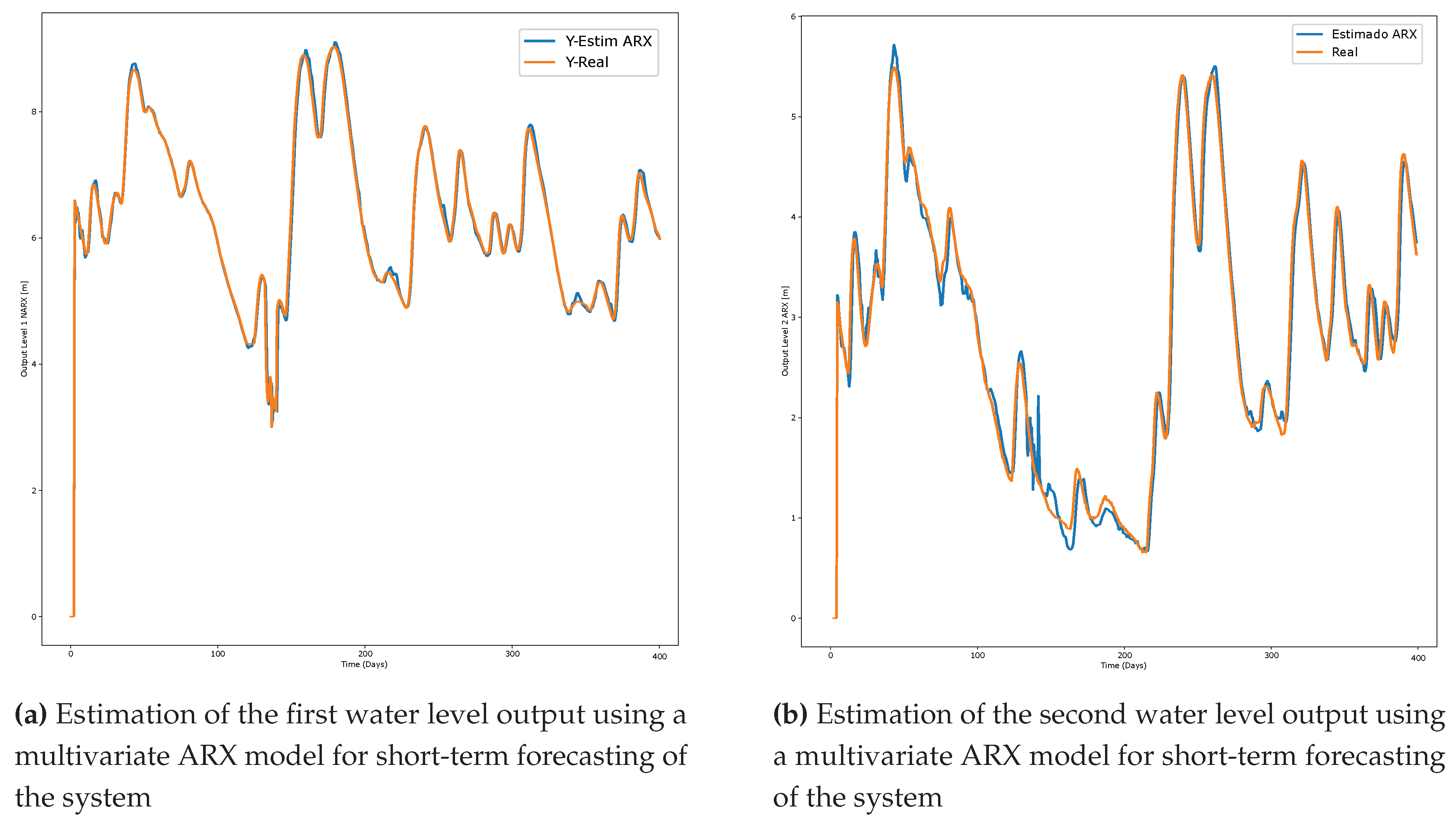
The results of the multivariate ARX method for both water level outputs are displayed in Figure 10, utilizing 64 nodes in the hidden layer according to the details in Table 3. Specifically, Figure 10 shows the short-term estimation of the first water level output, compared to the actual measurements. Furthermore, Figure 10 presents the short-term water level forecasting for the second output, along with the corresponding real measurements.

Evaluating the prediction outcomes depicted in Figure 8, Figure 9, and Figure 10, the proposed LSTM multivariate nonlinear neural network (NNN) exhibits satisfactory performance upon visual inspection, mathematical computation of root mean square error (RMSE), the Nash-Sutcliffe efficiency coefficient (NSE), and the computational runtime of the algorithm. To discern which approach most accurately captures the dynamics of the proposed model, a quantitative assessment is conducted. The mean square error is calculated for each considered method to compare actual measurements with their corresponding forecasts. The results of the mean square error for the multivariate LSTM approach are presented in the table. It is evident that the estimation error of the proposed LSTM model is lower than that of other models. Furthermore, the NSE coefficient value is closest to 1, aligning with the proposed theory that estimation is excellent when its value approaches 1.

In Table 2 is shown an analysis Regression metric data for the most relevant squared error estimates of the nonlinear recurrent neural network LSTM and the nonlinear neural network NARX.

Table 2. Mean squared Estimation (RMSE) and Nash-Sutcliffe efficiency coefficient (NSE) for a system long short-term.

Non-linear models	RMSE Output 1	RMSE Output 2	NSE Output 1	NSE Output 2
LSTM	0.0067	0.0028	0.9990	0.9991
NARX	0.0052	0.0060	0.9990	0.9983
ARX	0.0275	0.0071	0.9972	0.9980

From Table 2 It is observed that the total estimation error of the LSTM recurrent neural network is less than the estimation error of the NARX, and ARX neural network, furthermore it is observed that the Nash-Sutcliffe Efficiency coefficient of the LSTM recurrent neural network is closer to 1, which means that the proposed LSTM neural network model is better in terms of the other two neural networks with which the model validation is performed.

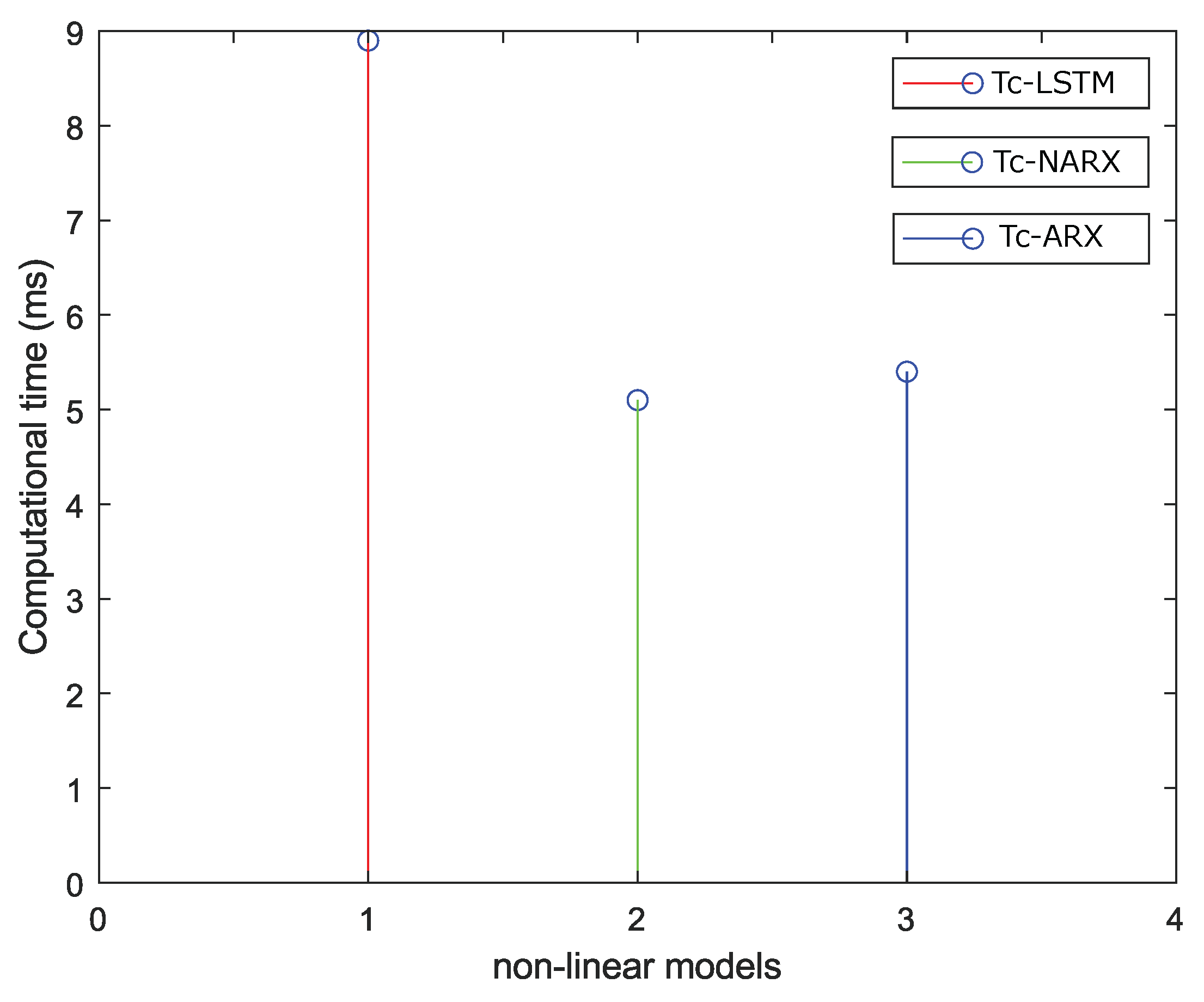
In Table 3 shows the computational execution time of the nonlinear neural network algorithm, in order to show that the LSTM recurrent neural network (RNN) model validated with the NARX and ARX neural networks do not require much computational work from the machine’s memory.

Table 3. computational execution time.

Non-linear models	Tic - Toc (s)
LSTM	0.0089
NARX	0.0051
ARX	0.0054

Figure 11 shows the response of the computed execution time for the (RNN) LSTM model in the short term, the computed time of the feed-forward neural network (NARX) and the computed time of the ARX model. It can be stated that for the (RNN) LSTM model, the algorithm requires more execution time due to its structure and operation of this type of networks since it is a long time, for the NARX model it requires less computation time due to its feed forward structure and the ARX model also in its execution time requires little time at the time of obtaining the results of the algorithm. For example, for the RNN LSTM the execution time is

0.0089

s, while for the NARX model the execution time is

0.0051

s, which means a reduction of the computational time of 57.3%. However, as shown in Figure 11, it can be seen that the computational time for all three models raised is quite low.

In Table 4 The model parameters of the nonlinear neural networks LSTM, NARX, ARX, used to train and test the models are shown.

3.3. Forecast Future Time Steps Based on the Predictions and Forecast of Future Time Steps Based on Measurements

Time series are used for chronologically ordered sequences of data, in principle equally spaced in time. Forecasting is the process of predicting future values of a time series based on previously observed patterns (autoregressive) or by including external variables and forecasting future time series values based on measurements from the LSTM recurrent neural network (RNN) model.

The results obtained for the two outputs of the proposed LSTM model are presented below in order to forecast future time steps based on the predicted and based on measurements RMSE and NSE metric regression measurements and estimation responses.

In Figure 12 forecasting future time series values of the LSTM recurrent neural network (RNN) model based on previously observed patterns (autoregressive), or including external variables. In Figure 12 the estimation of the first output of the water level of future time series values of the LSTM recurrent neural network (RNN) model is presented. In Figure 12 the estimation of the second output of the water level of future time series values of the LSTM recurrent neural network (RNN) model is presented.

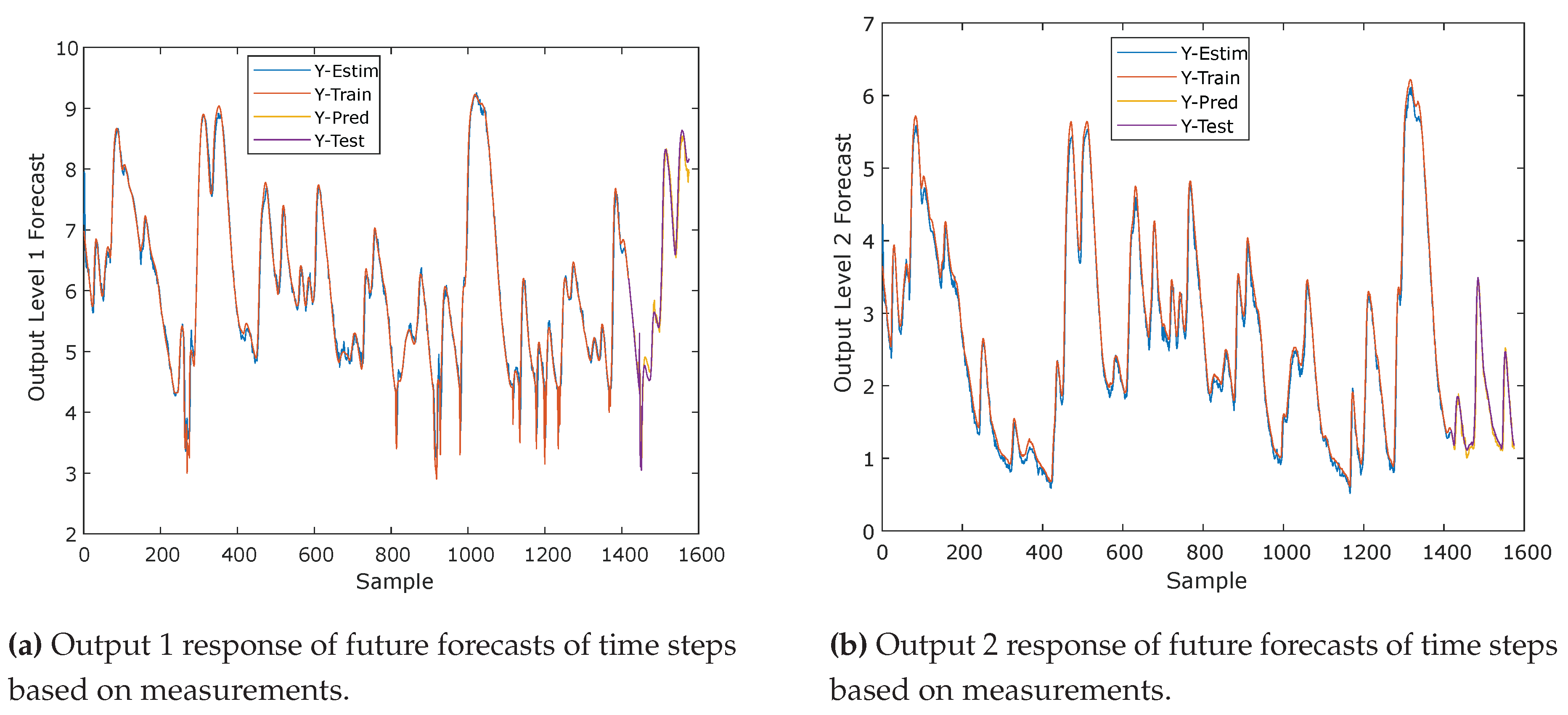
In Figure 13 Forecasting future time series values based on measurements from the LSTM recurrent neural network (RNN) model. In Figure 13 Output 1 forecasting response of future time steps based on measurements.In Figure 13 Output 2 forecasting response of future time steps based on measurements.

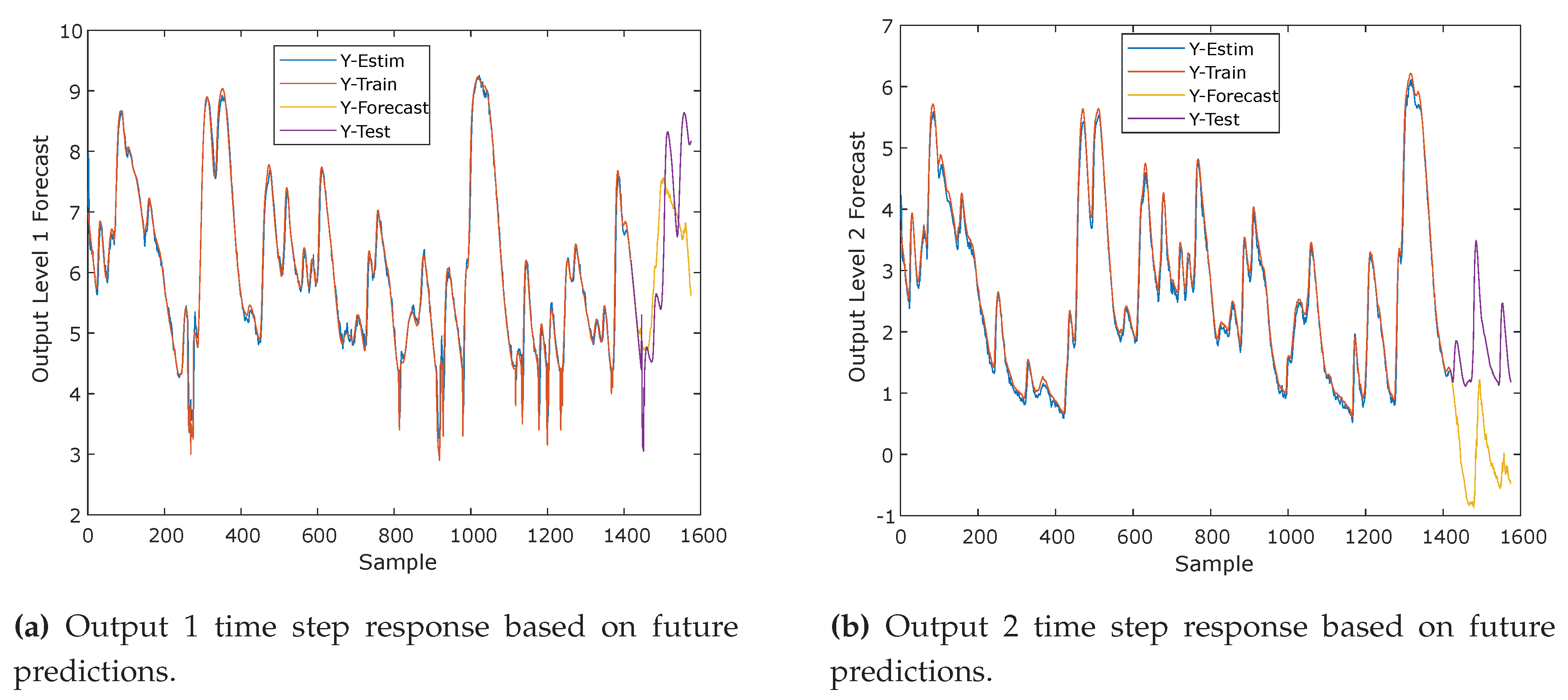
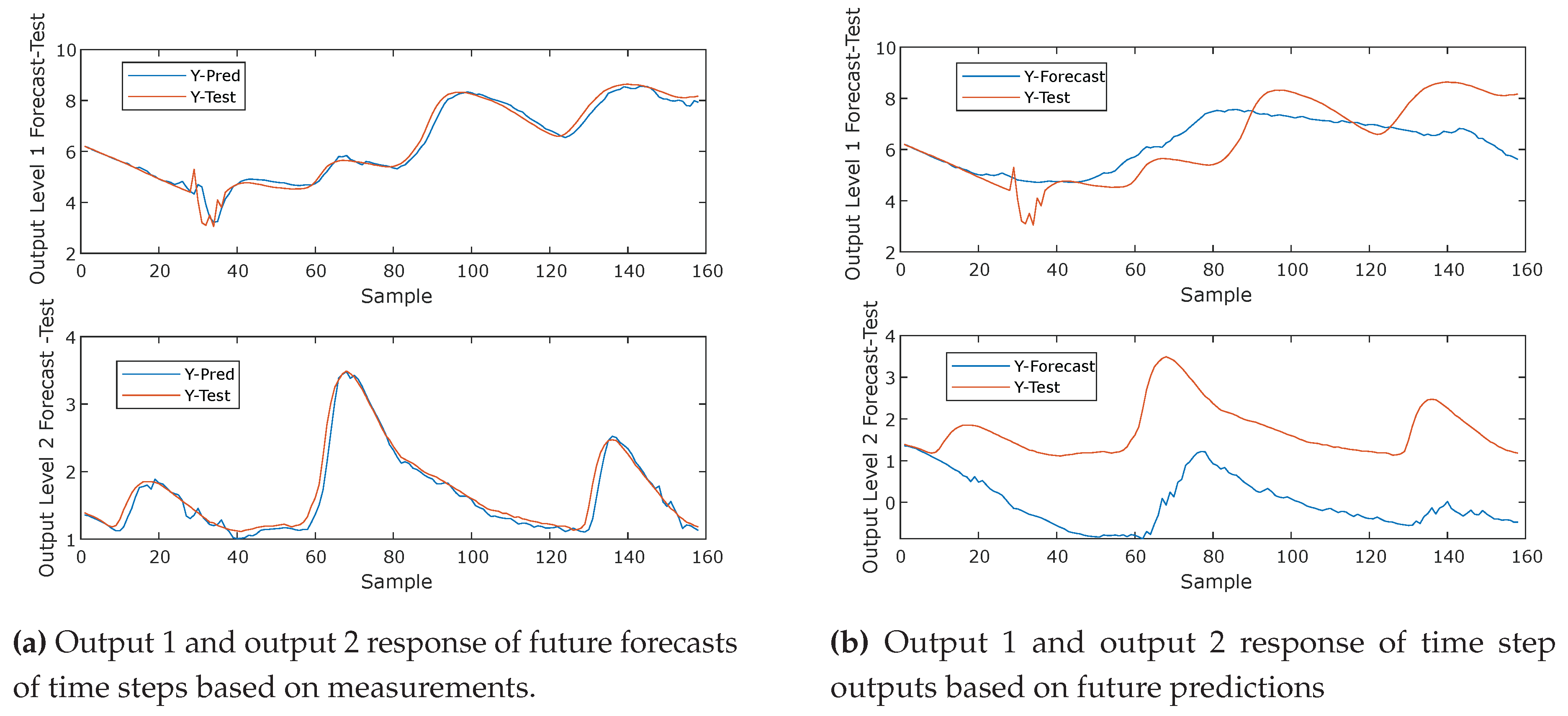
In Figure 14 Forecasting future time series values based on measurements from the LSTM recurrent neural network (RNN) model and response of time step based on future predictions. In Figure 14 Response of time step output 1 and output 2 based on future predictions.In Figure 14 Output 1 and output 2 forecasting response of future time steps based on measurements.

In Table 5 An analysis of two metric regression measures for the LSTM neural network of future forecasts and future forecasts based on the measurements is shown.

From Table 5 It is observed that the total estimation error of the LSTM recurrent neural network of future forecasts is larger than the estimation error of the LSTM neural network of future forecasts based on actual measurements, furthermore, it is observed that the Nash-Sutcliffe Efficiency coefficient of the LSTM recurrent neural network of future forecasts based on actual measurements closer to 1, which means that the proposed LSTM neural network model is very good for both short-term and long-term predictions.

4. Conclusions

The study at hand aims to develop a flood prediction model utilizing data collected from two hydrological stations situated along the Atrato River in the department of Chocó, Colombia. A meticulously constructed LSTM neural network model is employed to forecast the river level based on short-term models at these two hydrological stations. Unlike conventional hydrological models that require various input data such as flow, precipitation, and topography, the proposed algorithm solely utilizes measured data from the two hydrological stations on the Atrato River to predict future data regarding the river levels.

The LSTM model effectively learns the long-term dependencies between sequential data series and demonstrates reliable performance in flood forecasting, alongside two other neural network models evaluated in the research.

Parameters are defined to evaluate the model’s performance in predicting river levels at the two hydrological stations and to analyze the influence of input data characteristics on the model’s flood forecasting capability. Validation and testing of the proposed model are conducted using criteria such as the Nash-Sutcliffe Efficiency (NSE) value and the Root Mean Square Error (RMSE) value. The LSTM model is assessed for both short and long-term level forecasts using independent datasets for level, flow, and precipitation.

During both validation and testing phases, the LSTM model exhibits commendable performance. Notably, there are no significant differences in the simulation results for the three flow forecast cases with the LSTM model. However, concerning flood predictions, the NSE coefficient indicates slightly superior outcomes.

It is evident from Table 3 that the LSTM neural network necessitates more computational time compared to the other two nonlinear neural network models, NARX and ARX. This disparity arises because LSTM enables Recurrent Neural Networks (RNNs) to retain input information over prolonged durations. Unlike traditional RNNs, LSTMs possess the capability to store information in memory, allowing neurons to read, write, and erase data from their memory.

In conclusion, the presented LSTM multivariate model, based on recurrent neural networks (RNN), emerges as a valuable asset for predicting water levels, effectively capturing correlations among multiple hydrological variables and stations. The significant contribution of this study lies in the development of a versatile modeling framework that can be expanded to encompass various hydrological systems, incorporating additional stations and variables as needed.

Future research endeavors could delve into areas such as online training methodologies, white-box modeling approaches, or the application of more sophisticated nonlinear structures to enhance the model’s capacity in capturing the system’s inherent nonlinear behavior. These avenues hold promise for further advancing flood prediction capabilities and refining water resource management strategies.

The LSTM model employed in this study emerges as a robust tool for predicting water levels in hydrological systems, effectively addressing the complexities of correlated variables and multiple monitoring stations. The significance of this approach lies in its adaptable modeling structure, offering versatility for application to diverse hydrological systems with varying stations and variables. Future research directions may explore aspects such as real-time training, employing white-box models, or incorporating more sophisticated nonlinear structures to enhance the model’s capacity in capturing intricate nonlinear behaviors within the system.

References

Ciaburro, G.; Venkateswaran, B. Neural Networks with R: Smart models using CNN, RNN, deep learning, and artificial intelligence principles; Packt Publishing Ltd, 2017.
Muncharaz, J.O. Comparing classic time series models and the LSTM recurrent neural network: An application to S&P 500 stocks [Comparativa de los models clásicos de series temporales con la red neuronal recurrente LSTM: Una aplicación a las acciones del S&P 500]. Technical report, 2020.
Fleuret, F. The Little Book of Deep Learning. A lovely concise introduction 2023.
Le, X.H.; Ho, H.V.; Lee, G.; Jung, S. Application of long short-term memory (LSTM) neural network for flood forecasting. Water 2019, 11, 1387. [Google Scholar] [CrossRef]
Zhang, Y.; Gu, Z.; Thé, J.V.G.; Yang, S.X.; Gharabaghi, B. The Discharge Forecasting of Multiple Monitoring Station for Humber River by Hybrid LSTM Models. Water 2022, 14, 1794. [Google Scholar] [CrossRef]
Won, Y.M.; Lee, J.H.; Moon, H.T.; Moon, Y.I. Development and application of an urban flood forecasting and warning process to reduce urban flood damage: A case study of Dorim River basin, Seoul. Water 2022, 14, 187. [Google Scholar] [CrossRef]
Akbari Asanjan, A.; Yang, T.; Hsu, K.; Sorooshian, S.; Lin, J.; Peng, Q. Short-term precipitation forecast based on the PERSIANN system and LSTM recurrent neural networks. Journal of Geophysical Research: Atmospheres 2018, 123, 12–543. [Google Scholar] [CrossRef]
Adaryani, F.R.; Mousavi, S.J.; Jafari, F. Short-term rainfall forecasting using machine learning-based approaches of PSO-SVR, LSTM and CNN. Journal of Hydrology 2022, 614, 128463. [Google Scholar] [CrossRef]
Rahimzad, M.; Moghaddam Nia, A.; Zolfonoon, H.; Soltani, J.; Danandeh Mehr, A.; Kwon, H.H. Performance comparison of an LSTM-based deep learning model versus conventional machine learning algorithms for streamflow forecasting. Water Resources Management 2021, 35, 4167–4187. [Google Scholar] [CrossRef]
Hu, Y.; Yan, L.; Hang, T.; Feng, J. Stream-flow forecasting of small rivers based on LSTM. arXiv 2020, arXiv:2001.05681 2020. [Google Scholar]
Moishin, M.; Deo, R.C.; Prasad, R.; Raj, N.; Abdulla, S. Designing deep-based learning flood forecast model with ConvLSTM hybrid algorithm. IEEE Access 2021, 9, 50982–50993. [Google Scholar] [CrossRef]
Baek, S.S.; Pyo, J.; Chun, J.A. Prediction of water level and water quality using a CNN-LSTM combined deep learning approach. Water 2020, 12, 3399. [Google Scholar] [CrossRef]
Barzegar, R.; Aalami, M.T.; Adamowski, J. Coupling a hybrid CNN-LSTM deep learning model with a boundary corrected maximal overlap discrete wavelet transform for multiscale lake water level forecasting. Journal of Hydrology 2021, 598, 126196. [Google Scholar] [CrossRef]
Noor, F.; Haq, S.; Rakib, M.; Ahmed, T.; Jamal, Z.; Siam, Z.S.; Hasan, R.T.; Adnan, M.S.G.; Dewan, A.; Rahman, R.M. Water level forecasting using spatiotemporal attention-based long short-term memory network. Water 2022, 14, 612. [Google Scholar] [CrossRef]
Shuofeng, L.; Puwen, L.; Koyamada, K. LSTM based hybrid method for basin water level prediction by using precipitation data. Journal of Advanced Simulation in Science and Engineering 2021, 8, 40–52. [Google Scholar] [CrossRef]
Jabbari, A.; Bae, D.H. Application of Artificial Neural Networks for accuracy enhancements of real-time flood forecasting in the Imjin basin. Water 2018, 10, 1626. [Google Scholar] [CrossRef]
Tabbussum, R.; Dar, A.Q. Comparative analysis of neural network training algorithms for the flood forecast modelling of an alluvial Himalayan river. Journal of Flood Risk Management 2020, 13, e12656. [Google Scholar] [CrossRef]
Dtissibe, F.Y.; Ari, A.A.A.; Titouna, C.; Thiare, O.; Gueroui, A.M. Flood forecasting based on an artificial neural network scheme. Natural Hazards 2020, 104, 1211–1237. [Google Scholar] [CrossRef]
Abdullahi, S.I.; Habaebi, M.H.; Malik, N.A. Flood disaster warning system on the go. 2018 7th International Conference on Computer and Communication Engineering (ICCCE). IEEE, 2018, pp. 258–263.
Kimura, N.; Yoshinaga, I.; Sekijima, K.; Azechi, I.; Baba, D. Convolutional neural network coupled with a transfer-learning approach for time-series flood predictions. Water 2019, 12, 96. [Google Scholar] [CrossRef]
Graves, A.; Schmidhuber, J. Framewise phoneme classification with bidirectional LSTM and other neural network architectures. Neural networks 2005, 18, 602–610. [Google Scholar] [CrossRef]
Hochreiter, S.; Schmidhuber, J. Long short-term memory. Neural computation 1997, 9, 1735–1780. [Google Scholar] [CrossRef]
Cho, M.; Kim, C.; Jung, K.; Jung, H. Water level prediction model applying a long short-term memory (lstm)–gated recurrent unit (gru) method for flood prediction. Water 2022, 14, 2221. [Google Scholar] [CrossRef]
Renteria-Mena, J.B.; Plaza, D.; Giraldo, E. Multivariable NARX Based Neural Networks Models for Short-Term Water Level Forecasting. Engineering Proceedings 2023, 39. [Google Scholar] [CrossRef]
Kassambara, A. Machine learning essentials: Practical guide in R; Sthda, 2018.

Figure 1. Multivariable Structure of Long Short-Term Memory (LSTM).

Figure 2. Architecture of a regression LSTM neural network.

Figure 3. Data flow structure in time unit t.

Figure 4. Neural Network Architecture Utilizing the NARX Model.

Figure 5. ARX Structure.

Figure 6. Description of the Hydrological Station.

Figure 7. The location of hydrological stations in the Atrato River.

Figure 8. Multivariable LSTM forecasting results for two water level outputs for a system long short-term.

Figure 9. Multivariable NARX forecasting results for two water level outputs for a system short-term.

Figure 10. Multivariable ARX forecasting results for two water level outputs for a system short-term.

Figure 11. Computational time of model non-linear, LSTM, NARX , ARX.

Figure 12. Response of time step outputs based on future predictions.

Figure 13. Measurement-based future time step forecasting response.

Figure 14. Measurement-based future time step forecasting response outputs and response of time step outputs based on future predictions.

Table 1. Description of the hydrological station locations.

	Station 1 (E1)	Station 2 (E2)
Longitude	76° 40’ 10.75” W	76° 39’ 44.13" W
Latitude	5° 45’ 53.38” N	5° 41’ 52. 77" N
Altitude	20.579 M.A.S.L.	20.83 M.A.S.L.
City	Belén de Bajirá	Quibdó

Table 4. Model parameters of the nonlinear neural networks.

Non-linear models	Learning rate	# input nodes	# hidden nodes	# output nodes
LSTM	0.02	4	64	2
NARX	0.02	4	64	2
ARX	0.02	4	-	2

Table 5. Root mean square estimation (RMSE) and Nash-Sutcliffe coefficient of efficiency (NSE) for an LSTM system of future forecasts and future forecasts based on measurements

Non-linear model	RMSE Output 1	RMSE Output 2	NSE Output 1	NSE Output 2
LSTM Forecast-Future	1.2325	3.4520	0.3849	0.1234
LSTM Forecast-Measurements	0.0620	0.0160	0.9692	0.9894

Disclaimer/Publisher’s Note: The statements, opinions and data contained in all publications are solely those of the individual author(s) and contributor(s) and not of MDPI and/or the editor(s). MDPI and/or the editor(s) disclaim responsibility for any injury to people or property resulting from any ideas, methods, instructions or products referred to in the content.

© 2024 by the authors. Licensee MDPI, Basel, Switzerland. This article is an open access article distributed under the terms and conditions of the Creative Commons Attribution (CC BY) license (http://creativecommons.org/licenses/by/4.0/).

Copyright: This open access article is published under a Creative Commons CC BY 4.0 license, which permit the free download, distribution, and reuse, provided that the author and preprint are cited in any reuse.

MDPI Initiatives

Important Links

Choose an area of interest and we will send you notifications of new preprints at your preferred frequency.

Disclaimer