
Submitted:
02 April 2024
Posted:
03 April 2024
You are already at the latest version
Abstract
To understand how the thinning strategies impacts on wood quality and quantity for different purposes is of interest, considering that the management of plantations is carried out with parameters that have yet to be validated for different growth conditions. This work evaluated contrasting thinning regimes applied early at two moments of the crop cycle. With an initial population of 840 trees.ha-1, two thinning with populations ranging from 700 to 400, and from 400 to 100 trees.ha-1 were applied at 1.5 and 7.3 years, respectively. Growth analyses were carried out from the ages of 1.5 to 20.8 years considering: total height, diameter at breast height, individual volume, total and commercial volume per hectare, mean annual increase and current annual increase. At final age, contrasting populations of 100, 250 and 400 trees.ha-1 were sampled to assess wood density, and mechanical properties (bending and compression on small scale clear samples). The values of individual growth and wood properties are related to a Stand Density Index to understand the effect of competition on those values. The results allow us to identify the thinning schemes that record the most significant individual and per-hectare growth (both in thinning and clear felling) and the optimal harvest time under specific growth conditions. We assessed the proportions of commercial logs for sawmill and pulp uses, providing valuable inputs for a subsequent economic analysis of thinning regimes seeking for the most convenient combination of wood products. Wood's physical and mechanical properties assessed were barely affected by contrasting levels of competition between trees, therefore the decision of the silvicultural system to implement will depend on production and economic criteria.
Keywords:
Eucalyptus grandis
; thinning
; growth
; wood quality
; sawmill
1. Introduction
Management of even-aged stand requires setting production objectives according to required forest products. For many non-integrated foresters the aim is to manage plantations to obtain multiple products of higher and lower value for uses such as solid wood and pulp. Silvicultural decisions, including stand density management, need to be made considering cost/benefit relationships based on yield and wood quality, among other factors (e. g. markets and price). In the context of plantations in Uruguay the density ranges from 1000 to 1500 trees.ha-1 and is managed with thinnings up to 100 to 300 trees.ha-1 [1].
Reducing competition between individuals by removing smaller trees determines that growth factors such as water, light, and nutrients are concentrated in the individuals with the highest productive potential [2]. In thinned forests, individual growth increases due to a higher rate of photosynthesis in the middle and lower areas of the canopy associated with greater light penetration [3]. According to Medhurst and Beadle [4] this is particularly evident for species that are poorly tolerant to shading, although some authors claim that eucalyptus trees tolerate competition between individuals [5,6].
Having information on how these plantations should be managed to obtain high-quality products such as straight stems, large diameters and desirable wood properties (e.g. density, strength, fiber length) requires research for each situation [7]. High-quality wood is achievable by reducing competition between individuals by regulating the tree population. This determines that growth factors such as water, light, and nutrients are concentrated in the individuals with the highest productive potential [2]. The effects on growth are more evident in the diameter at breast height [8,9,10] and, therefore, in the basal area, compared to individual height, although the results reported on the latter indicate a variable response [11,12]. This effect on the growth rate of the remaining individuals tends to shorten the length of rotation, which is pursued from a financial point of view [13]. The economic income from the wood produced in commercial thinning, which essentially has a cellulosic destination must be considered of interest as well.
Site quality, age and size of the trees, and the proportion of trees removed are among the factors that have the most significant effect on the growth response to thinning [14,15,16,17]. Simultaneously, site quality is closely linked to the growth rate, which determines that the effects of a certain thinning are specific to each situation [18]. In sites of high forest quality, such as those in the northern area of Uruguay [19], it is expected that the response of the dominant trees will be high since they are more efficient than the smaller ones in the competition for light[18]. Considering the moment of thinning for commercial eucalypt species in general, it is observed that when this coincides with maximum growth rate (within the first five years), the most significant responses are achieved in terms of individual growth [15], considering the apparent absence of limiting factors such as water and nutrients [20]. According to Smith and Long [21] after a rapid initial growth, a decrease occurs due to a closure of the canopy, which coincides with the stage of maximum leaf area development. This occurs in the early years for many eucalypt species and represent an indicator of the moment to apply the first thinning to temporarily reduce the effects of competition between individuals.
Thinning intensity refers to the number of interventions carried out and the amount of trees removed in each operation expressed in terms of basal area, wood volume, or number of trees [22]. In most cases, very intense thinning leads to an unwanted increase in the size of the branches, which reduces the quality of the wood and a loss of volume per hectare, altering the tapering. On the other hand, light thinning determines an anticipated growth stagnation in addition to reduced diameters of little commercial value [9]. At both extremes, there is an underutilization of the potential of each site in terms of growth factors or some limitations for their expression [23]. As a tool to define density of stocking related to a maximum stocking capacity, Reineke [24] proposed a tool known as the stand density index (SDI). This index provides size-density relationships to help understanding the competition status of an even aged stand.
Wood properties for solid uses of eucalypt species in general are greatly influenced by the growth rate, which in turn depends on silvicultural practices [25,26], site characteristics such as temperature [27] and soil water availability [28]. However, some results show the lack of a relationship between wood quality and individual growth [29]. Wood density has been shown a very variable relationship with the growth rate with positive [30], negative [31], and neutral [32] associations between both parameters. The literature agrees in pointing out that the sapwood region of eucalyptus trees has greater density than the heartwood [25,33,34]. On the other hand, a positive relationship has been determined between the proportion of sapwood and the leaf area index [35]. As mentioned above, the leaf area index is directly related to the spacing between individuals. This depends on the shading tolerance shown by the different eucalyptus species [36]. However, contrary results were obtained by Wilkins [37] with very similar values of sapwood proportion in treatments without and with thinning at the age of 2.75 years (1089 and 479 trees.ha-1, respectively) in E. grandis.
The positive relationships between spacing and wood strength in eucalypt species are explained by the effect on wood density [38] and the microfibrillar angle [39,40]. Hein et al. [41] reported a combined and additive effect of the density and the microfibrillar angle (of the S2 wall) with a better capacity to predict the resistance properties of the wood than if they are considered individually. Lower values of the microfibrillar angle result in higher compressive strength, while higher values result in higher bending strength, which indicates that an ideal value will depend on the end use of the wood [42,43,44]. The variation in the angle of the microfibrils is associated with the proportion of late/early wood, juvenile/adult wood, and growth rate (among others). However, this is more evident in conifers than in broadleaf trees [43](Donaldson, 2008). The literature, in general, shows that high growth rates determine high values of the microfibrillar angle [28,44,45] and that an increase up to 16 degrees reduces density and MOE, while values above that have no appreciable effect [40]. This determines that the effects of thinning on the microfibril angle and the properties of the wood properties must be determined for each situation.
As a consequence of the above, we hypothesize that the different intensities of thinning affect productivity, harvest period, and wood properties in trees of harvest age. To understand the magnitude of this effect, the following objectives were proposed: i) to evaluate the response of different thinning combinations on individual and per hectare growth at rotation age, ii) to understand how thinning combinations affect the biologically optimum harvest age, iii) to quantify the impact effect of thinning on commercial wood, focusing on sawn and pulpwood and iv) evaluate the effect of contrasting stocking on physical and mechanical properties of the wood.
2. Materials and Methods
Our analysis is based on a thinning trial comprising 10 treatments. For analyzing the first and second objective we used thinning records and measures taken along the life of the trial to assess diameter breast height, total height, standard deviation of diameters, mortality, individual volume, volume per hectare, mean annual increment, and current annual increment. The third objective was assessed by applying a logging simulation model using information of each treatment at harvest age as inputs to quantify solid wood and pulp wood yielded by each treatment during commercial thinning and clear felling. For objective number four, we analyzed bending strength (b) and compression strength parallel to the fibers (c) by sampling trees from 3 of the 10 treatments. We extracted discs and specimens to measure modulus of elasticity (MOE), modulus of rupture (MOR) and wood basic density (ρ) in laboratory conditions. Stand Density Index (SDI) [24] were calculated for each treatment to understand the evolution of competition and its relationship with growth and wood properties. Finally, statistical comparisons of all the regimes regarding growth and wood properties were performed. Methodological details of those processes are shown below.
2.1. Study Area
The trial was installed in a commercial Eucalyptus grandis plantation (seminal origin) in December 2000 in northern Uruguay (Department of Rivera, 31°15' 30'' South latitude and 55° 40' 44" West longitude) (Figure 1).
Soils are reddish brown, sandy with high aluminum content, and very low natural fertility. Soil depth is greater than 1.2 m, providing a great water storage capacity [46]. Climate is temperate with average maximum and minimum temperatures of 24 and 12 °C, respectively. The average anually accumulated precipitation is 1600 mm [47]. Site index (key age = 10 years) is 31m, which corresponds to high growth rates.
Seeds to produce the seedlings were from Bañado de Medina Experimental Sation of the School of Agronomy, University of the Republic, in the department of Cerro Largo (northeast of Uruguay). For soil preparation, a clearing furrower (with symmetrical mouldboards), three chisels, and two hilling discs were used. Planting was carried out manually with a subsequent application of 100 and 120 g per plant of ammonium phosphate to both sides of the plant.
2.2. Experimental Design
The experiment comprised thinning regimes combining stocking densities during the first and second thinning applied at ages 1.5 and 7.3 years, respectively, ensuring that the remaining trees were homogeneously distributed in the plot (Table 1). The design was complete randomized blocks with 3 repetitions. Plots are composed of 8 rows of12 plants, planted at 4x2 m. In total 30 plots occupy 28,800 m (960 m2 each) with an initial stand density of 850 trees.ha-1 (See Figure S1 Supplementary material).
2.3. Growth and Competition
Diameter at breast height (DBH, cm, 1.3m) and total height (Ht, m) were measured for each tree. in 2002, 2005, 2007, 2008, 2009, 2011, 2015, 2018, 2019, and 2021. Total individual volume under bark (Vi, m3.tree) was estimated applying equation 1 [48], and the total volume per hectare (Vht, m3.ha-1) was calculated as the sum of individual volumes of each plot, related to one hectare.
Vht value extracted in the second thinning was estimated by multiplying the average Vi by the number of thinned trees in each plot.
Coeficient of variation of the diameters (CV, %) and the number of trees per hectare (N, trees.ha-1) were calculated to compare uniformity of individuals and mortality (Mo, %) dynamics along the rotation. Competition between individuals of each regime was assessed through Reineke’s SDI considering the slope of the self-thinning line as -1.605 as proposed by the author. The maximum SDI (SDImax) was set on 1200 trees per hectare according to Rachid (unpublished data), and relative density (RD) was calculated as (SDI/SDImax).100.
To estimate commercial volume per hectare (Vhc, m3.ha-1) for pulp and sawmilling uses, a simulation software was applied. The software initializes with stand characteristics and requirements of log dimensions for each category (pulp and sawmilling) to estimate diameter distributions and stems’ taper [48]. Log length considered was 5.3 m and small end diameters for pulp and sawmilling were 6 and 25 cm respectively.
2.4. Wood Properties
2.4.1. Weighted Basic Apparent Density
Basic density (Bd, g.cm-3) was analyzed at age 7.3 years (second thinning) and at 20.8 years. It was determined using the dry weight and green volume values of sampled stem discs according to the standard UNIT 237:2008 [49].
During the second thinning, 2 to 3 trees from each plot whose DBH was close to the mean of each plot were felled. Two discs were removed: one at breast height (1.3 m), and the second at 50% of the commercial height defined by a small end diameter of 6 cm over bark. Both discs were transported in closed nylon bags and placed in water on the same day to maintain saturation condition. Discs were kept submerged until a constant weight and the green volume of each piece was obtained by water displacement. Subsequently, discs were dried in an oven at 103 oC ± 2 until constant weight to obtain de dry weight.
For age 20.8 years 3 thinning regimes were selected to analyze the combination for the first and second thinning of 400-100, 550-250, and 700-400 remaining trees.ha-1, respectively. For all plots corresponding to those treatments, 4 individuals per plot were sampled according to DBH class: two trees corresponding to the mean class, one from the smaller class, and one from the largest class of each plot. A total of 36 individuals were sampled. Trees were felled and disc samples were extracted at heights of 3.3, 5.3, and 7.3 meters to determined Bd according to the same standard.
The weighted basic density (Bdw, g.cm-3) of each tree was estimated according to the following Eq. 2 [50]:
Where: Ai and Bdi are the surfaces and wood densities of the disks extracted at 3.3, 5.3, and 7.3 m, respectively.
2.4.2. Current Apparent Density
Current apparent density (Cd, g.cm-3), was assessed for age 21.8. From the same stems sampled for estimating Bdw, two logs of 1 m length located at 2.3 and 4.3 m height were extracted. Specimens from the intermediate position (50% in the radius) and from the north-south orientation were prepared of two dimensions: 25 * 25 * 100 mm and 25 * 25 * 400 mm (width, thickness, and length, respectively) (Figure 2). These samples were also used for bending and compression tests.
The 288 specimens (2 per log * 2 logs per tree * 2 dimensions * 36 trees) were conditioned at 20 °C and 65% of humidity for 20 days until constant mass was reached. The equilibrium moisture content was close to 12% at the end of conditioning. This moisture content was verified in 63 test specimens.
Each specimen's weight and volume were measured to determine the Cd according to the standard UNIT 237:2008 [49]. The Cd value of each tree was obtained as the average of the four specimens of each log.
2.4.3. Bending Strength
The mechanical tests were carried out on the 25x25x400 mm specimens in a universal testing machine with a maximum load capacity of 100 KN (Shimadzu AGS-100) with a load cell of accuracy of 0.5%. Procedure for estimating the static bending strength followed usual standards ASTM D 143-94; UNIT 1137:2007 [51,52].
Modulus of Elasticity (MOEb MPa) and Modulus of Rupture (MORb, MPa) were calculated, both in bending according to Eq. 3 and 4:
Where: ∆P = Range of load between two points of the elastic zone (N) typically 10 to 40% of maximum load were taken, L = span (mm), ∆d = Elongation (mm), I = moment of inertia (mm).
Where: P = maximum applied load (N), L = span (mm), b = width of the specimen (mm), h = height of the specimen (mm).
2.4.4. Compression Strength Parallel to the Fibers
Measurement of the compressive strength was carried out using the smallest specimens in the same equipment and according to the standards ASTM D 143-94; UNIT 1137:2007 [51,52]. Modulus of Elasticity (MOEc, MPa) and Modulus of Rupture (MORc, MPa) were calculated, both in compression according to Eq. 4 and 5:
Pmax is the maximum load attained during each test, ΔP/ΔL is the slope of the load-displacement curve between 10 and 40% of the maximum load reached during the test, Lo is the initial length of the specimen, and Ao is its initial cross section area.
2.5. Statistical Analysis
To assess the effect of the different regimes on the range of variables of interest an analysis of variance was undertaken according to the following model Eq. 6:
Where Y ij is the variable measured in the plot for each thinning I, in block j; μ is the overall mean of trial; ei is the effect of thinning (fixed effect); βj is the j effect of the block; and εij is the experimental error associated with each observation (assumed to be independent and with a normal distribution of mean 0 and variance σ2).
The variables analyzed were DBH, Ht, Vi, Vht, Bbp, Cd, MOFb, MORb, MOEc, and MORc at age of 20.8, and Vht and Bdw at the age of 7.3 years.
Normality of the residuals and homogeneity of the variances were verified with the Shapiro-Wilk and Brown-Forsythe tests, respectively, whereas the distribution of the errors was checked through graphic analysis. In cases where these assumptions were not verified, the Kruskal-Wallis test was used. Subsequently, comparisons of means were carried out using the Bonferroni and SNK tests or growth variables and Tukey tests for wood property variables.
Correlations between Cd/Bdw vs. MOFf, MORf, MOEc, and MORc were analyzed through the Pearson test using the values of each stem sampled.
3. Results
3.1. Individual Growth
The growth curve of DBH and Ht shows a change in the behavior of both variables from the moment of second thinning onwards, from which the differences between thinning schemes increase (Figure 3). This response is more significant compared to the first thinning at 1.3 years. The differences at rotation age (20.8) are comparatively greater in the DBH than in Ht, with maximum and minimum values at lowest and highest densities, respectively. The final populations of 200 and 300 trees.ha-1, whose initial densities were 400-550 and 550-700, respectively, show very similar growth at the end of the evaluation period. Vi follows DBH behaviour due to its greater weight compared to Ht (Figure 3). For the individual variables, a relative stagnation in growth rates is observed after 18 years of age. DBH variation (CV) observed differs between thinning regimes. Populations with more than 300 trees.ha-1 showed more variation (between 70 to 90 % of the mean). Whereas regimes with less than these population showed less variation in DBH. However, the most severe thinning regime showed higher variation as well at the final age. The analysis of variance at the age of 20.8 years indicates significant differences for the three mentioned variables (Table 2). However, densities with differences of 50 trees.ha-1 showed small variation in individual growth considering final densities of 100 to 150 trees.ha-1. For those stockings the mean DBH is greater than 50 cm. On the other hand, the smallest DBH and Vi are recorded in the population without thinning. At the same time, mean height remain similar in contrasting stockings such as300 and. 800 trees.ha-1.
3.2. Productivity per Hectare and Competition Level
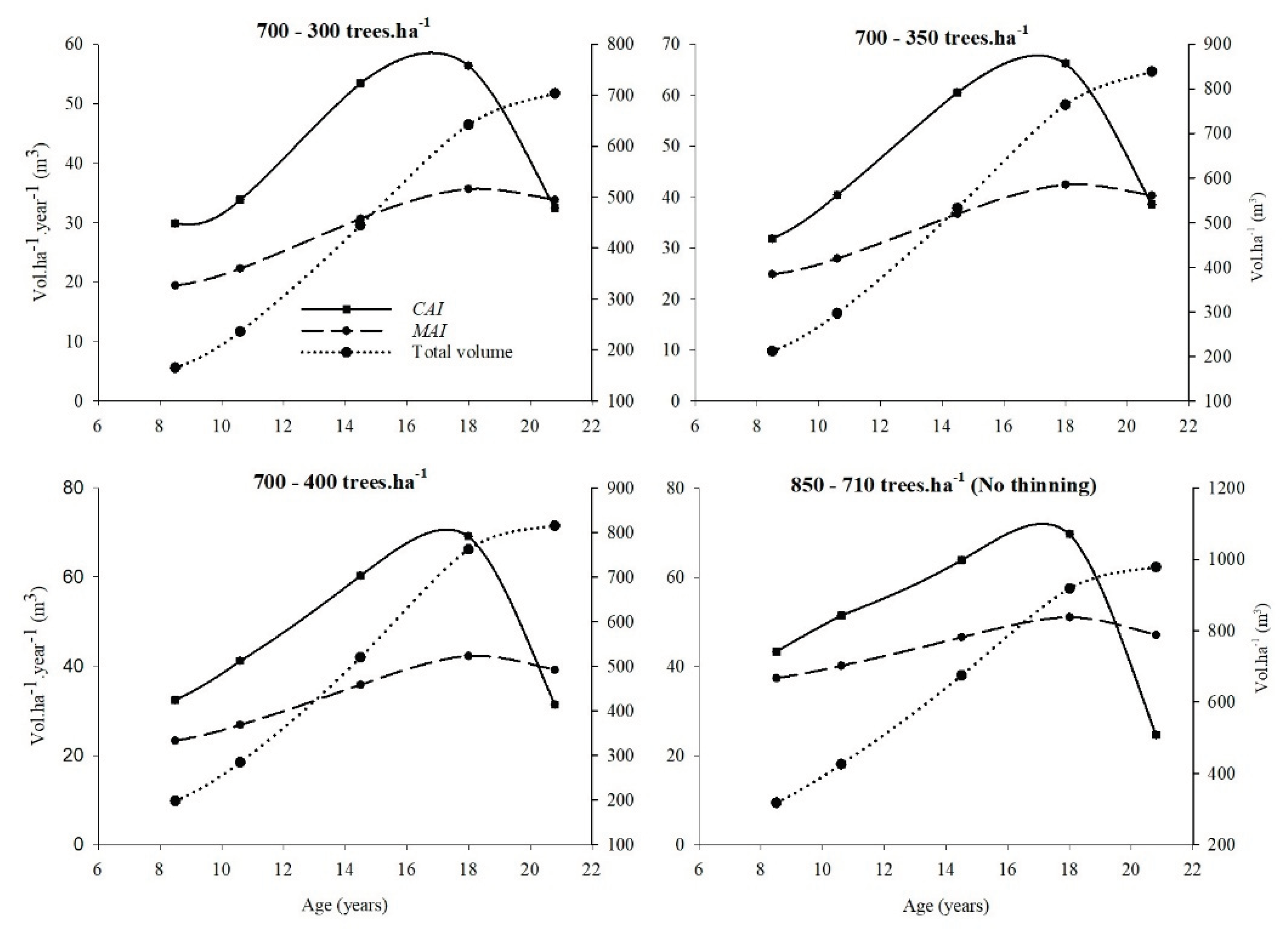
The evolution of the Vht shows that treatments with largest populations doubles the volume of regimes with smallest remaining populations A notable decrease in the growth rate after 18 years of age is also observed for all the regimes (Figure 4). The Mo showed increasing levels until the second thinning but without any relationship with the tree populations. The reduction in the number of trees that occurred in the second thinning determines a rapid drop in the loss of trees which subsequently recovers the levels prior to this moment. In all cases, relatively low values of Mo are observed except for populations with 400 – 100 trees.ha-1 and the control without thinning. The analysis of MAI-CAI curves indicates that the biologically optimal harvest age differs little between stockings and occurs around the age of 20 years (Figure 5a, 5b, and 5c).
Figure 4.
Vht and Mo for all the thinning regimes evaluated.
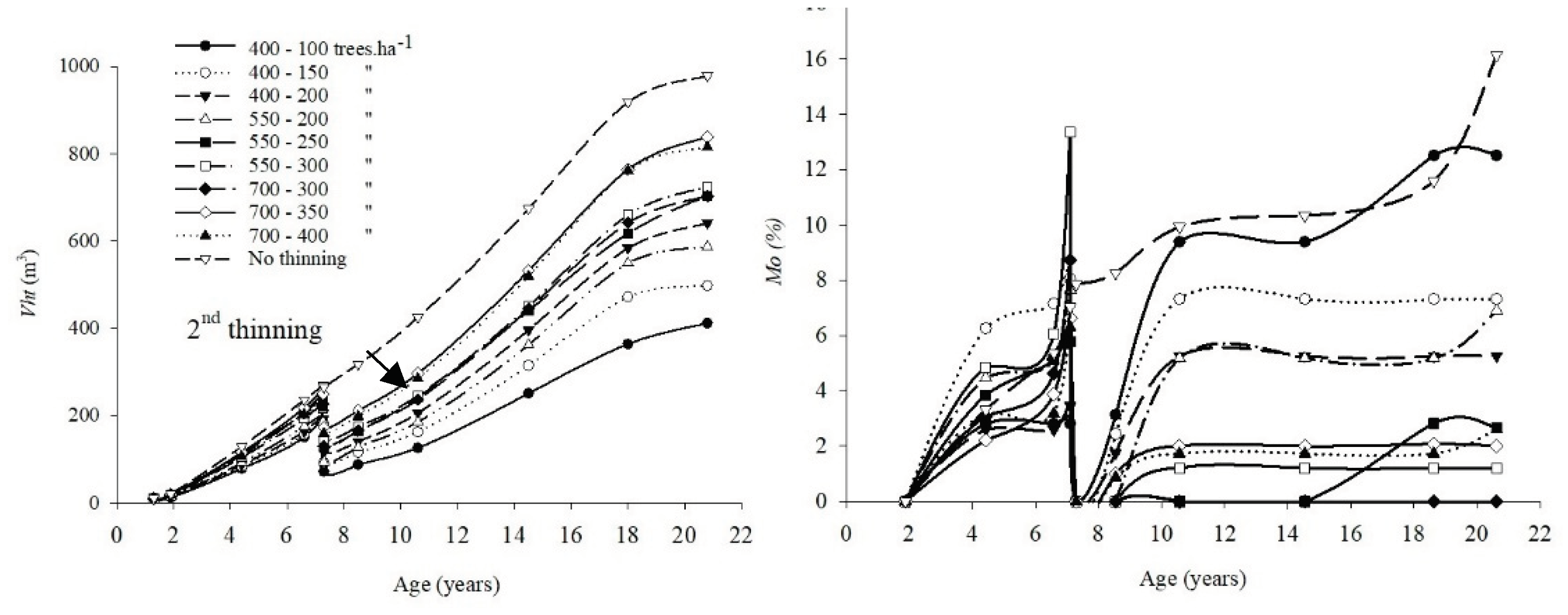
Figure 5a.
MAI-CAI curves and Vht of thinning regimes of 400-100, 400-150, and 400-200 trees.ha-1 until 20.8 years.
Figure 5a.
MAI-CAI curves and Vht of thinning regimes of 400-100, 400-150, and 400-200 trees.ha-1 until 20.8 years.
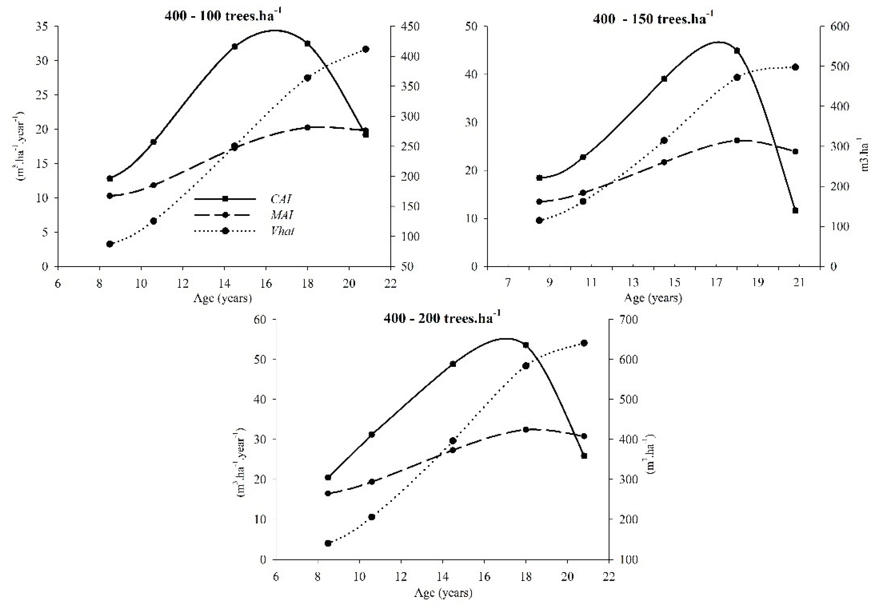
Figure 5b.
MAI-CAI curves and Vht of thinning regimes of 550-200, 550-250, and 550-300 trees.ha-1 until 20.8 years.
Figure 5b.
MAI-CAI curves and Vht of thinning regimes of 550-200, 550-250, and 550-300 trees.ha-1 until 20.8 years.
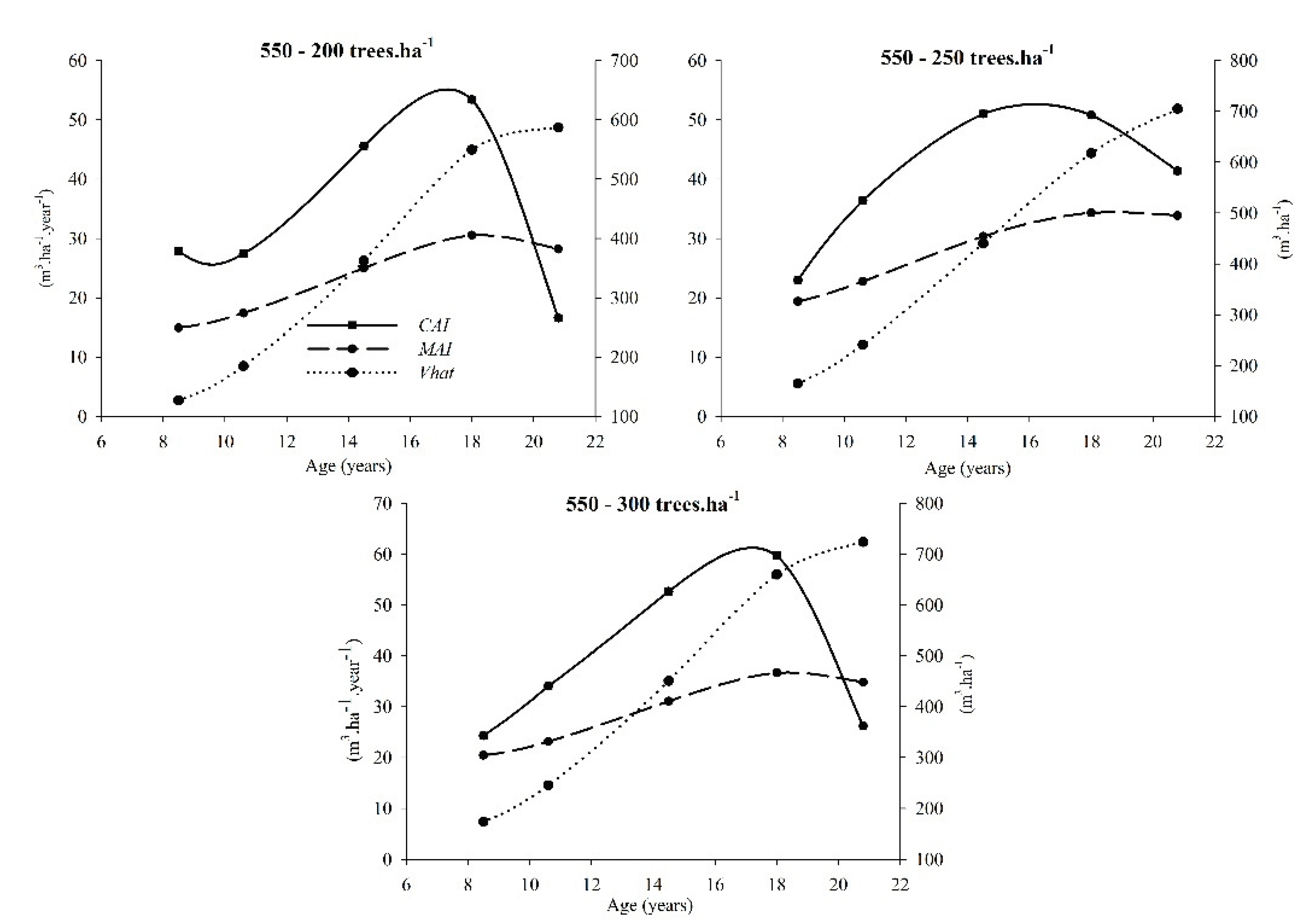
Figure 5c.
MAI-CAI curves and Vht of thinning regimes 700-300, 700-350, 700-400 trees.ha-1 and No thinning until 20.8 years.
Figure 5c.
MAI-CAI curves and Vht of thinning regimes 700-300, 700-350, 700-400 trees.ha-1 and No thinning until 20.8 years.
As expected, total volumes harvested in the second thinning were the larger in regimes with most significant reduction in the number of individuals, such as the regimes 400-100, 550-250/200, and 700-300. An inverse trend is recorded with the values obtained at harvest age and total wood harvested (Table 3). A joint plot of Vht and DBH is performed to understand the relationship between the total volume of wood, and trees fulfilling the requirement of large diameter for sawmilling industries. An inverse relationship between both variables was observed, with final densities of approximately 250 trees.ha-1, which would provide relatively high wood yields and diameter values (Figure 6).
Regarding competition, the first intervention was performed when the population was theoretically in free growth, suggesting it was an early thinning. At the age of the second thinning, two regimes with the lowest population were still in free growth, while the remaining regimes were in the stage corresponding to increasing competition. None of the regimes were fully stocked. At harvest age (20.8 years), only the regime 400-100 remained in theoretical free growth, the least severe regimes denoted fully stocked populations whereas the intermediate regimes where in increasing competition (Table 4).
Regarding to the Vhc for the second thinning, for all thinning regimes log dimensions fulfilled requirements only for pulpwood dimensions. (Table 5). The proportion of logs for cellulose and sawmill at harvest age is variable among thinning combinations. Regimes with final stand densities of 100 to 300 trees.ha-1 provided over 70% of wood for sawmilling. In the case of the treatment No thinning this proportion was close to 50%. Considering the total commercial volume (including thinning and harvest) very similar yields of wood for sawmilling are recorded comparing final densities of 100 and 200 trees.ha-1 (close to 70%).
3.3. Wood Properties
3.3.1. Basic Apparent Density and Current Apparent Density
The analysis of the Bdw and Cd variance shows significant differences between final densities of 100, 250, and 400 trees.ha-1 (Figure 7). Combination of thinning 400-100 trees.ha-1, recorded larger Bdw and Cd. The largest variability of the data is observed for this thinning, probably associated with the largest amount of specimens extracted from different positions in the logs.
The increase of Bdw from the second thinning to harvest age was similar in magnitude among lower final stockings (400-100 and 550-250 trees.ha-1), whereas Bdw remained unchanged for higher stockings (700-400 trees.ha-1) throughout the analyzed period (7.3 to. 20.8 years of age) (Figure 8).
3.3.2. Mechanical Properties
3.4. Relationship between Density and Mechanical Properties
The correlation values between Cd and Bdw and the mechanical properties of the wood indicate that the highest values (and in all cases significant) are obtained with the first of the mentioned densities except for MOEc (Table 6 y Figures S2-S4 Supplementary material). The lower values obtained with the Cd are explained since all the variables were measured in the identical specimens, unlike the Bdw measured in the discs. A strong correlation value was also obtained between the density of the wood measured in test pieces and in discs despite coming from different positions in the log.
4. Discussion
Our work was oriented to understand growth and wood properties of Eucalyptus grandis growing in excellent site conditions (SI=31m at 10 years) at different thinning regimes, that combine a wide range of stockings. The analysis was extended to the lifespan of the stand, allowing to visualize the optimal harvest age considering total and commercial volume (for sawmilling and pulp), along with wood quality for solid uses. To relate our results to state of competition of the stands, we used the SDI as applied by Reineke [24]. Results confirm the hypothesis that contrasting thinning combinations affect the growth and some properties of the wood of E. grandis. Implementing thinning regimes on a commercial scale will be subject to costs and projections of market prices for each type of product, particularly for the diameters of the basal logs. Therefore, it is necessary to identify regimes that combine individual growth and yield per hectare in search of the best economic result for each particular commercial scenario.
4.1. Individual Growth
The first thinning was performed at the age of 1.3 years when SDI values indicate the lack of competition between individuals. However, competition started at age 4 for regimes with 700 trees.ha-1, and two years later for regimes with 400 to 550 trees.ha-1 so that at the time of the second thinning, different levels of competition provided a first differentiation in DBH but no in Ht. Prior to the second thinning contrasting populations of 850 and 400 trees.ha-1 presented differences of 4.4 cm. After the second thinning, the large span thinning intensities applied provided a range of competition levels so that at harvest age the difference in the average DBH values between densities of 700 opposed to 100 trees.ha-1 was over 22 cm. A larger DBH at the end of the cycle obtained with lower stockings has been reported by several authors [10,53,54]. Ferraz Filho et al. [55] observed that the largest diameters were achieved with final densities of 150 trees.ha-1 (at age 11 years) and when the first thinning was applied sooner (at age 2.5 year) for the same species. However, in all treatments, a change in the growth rate was observed from year 11 onwards.
The analysis shows that with populations of 100 and 200 trees.ha-1 DBH values greater than 45 cm can be achieved,. Comparing different paths to final densities of 200 trees.ha-1, populations of 550 and 400 trees.ha-1 prior to thinning did not result in differences regarding individual diameters at harvest age. This range of final densities has also been evaluated for eucalyptus species, seeking to identify thinning combinations that allow high individual growth rates [11](J. Medhurst et al., 2001).
In our analysis we checked the little response of dominant trees to thinning due to a more significant relationship with site quality than with silvicultural practices. This determines that no statistical differences regarding DBHdom were detected between final populations of 100 and 400 trees.ha-1 (52.7 and 45.7, respectively). There is evidence that these trees have greater efficiency in capturing light and are little affected by competition with neighbors [56,57]. In this way, it is possible to obtain a certain number of trees with large diameters of trees growing at wide range of densities [18,58].
Growth of Ht prior to the second thinning shows a difference of 2.2 m between contrasting densities (800 and 400 trees.ha-1), representing a minor variation compared to DBH. The reduced variation in the different thinning schemes was reported by Schönau [59]. Smaller spacings promote the occurrence of dominated trees, which determines a reduction in their size [60]. However, in some cases, an inverse relationship occurs, explained by the high competition for light [61]. The latter probably occurs with closer spacings than in the ones analyzed in this work.
As opposed for the DBH, growth rate decreases from year 18 onwards for all treatments except for the treatment without thinning, which begins sooner. This is probably due to a greater competition for resources. From this age onwards, a certain reduction occurs, which may be due to stagnation in growth in Ht added to the intrinsic error in the measurement equipment for this variable since no tree death occurred. Lack of differences in Ht for final populations between 100 to 350 trees.ha-1 are consistent with the results of other authors evaluating similar thinning regimes for eucalypt species [11,12].
Behavior of Vi is very similar to DBH in terms of the differential response in time after the second thinning. However, the difference between the extreme densities is almost three times (1.5 vs 4.2 m 3.tree-1). These differences are due to more significant growth in diameter and height that occurs at larger spacings. Similar relationships were obtained by Scheeren et al. [23] and Trevisan [62] evaluating eucalypt species with final tree densities equivalent to this study's.
Considering the contrasting competition status at final age indicated by the SDI between No thinned populations (810 trees.ha-1, fully stocked and imminent mortality) and heavily thinned treatments (100 trees.ha-1, in transition between free growth and increasing competition), the differences recorded in individual growth are 1 to 3 times.
4.2. Productivity per Hectare
Due to the different reductions in tree populations in the first and second thinning, Vht differs substantially between treatments. As expected, the populations with the largest stocking register the largest volumes. A similar response was obtained by Trevisan [62] evaluating E. grandis at 18 years of age with final densities of 800 to 200 trees.ha-1. The results obtained in this study show that increases in tree densities do not translate in the same proportion to productivity per hectare, as reported in the literature [53,63]. In this case, population 8 times larger determines basal area 2.7 times larger and almost 2.5 times volume (412 vs 978 m3.ha-1).
For all thinning regimes a decrease in the growth rate is observed from 18 years onwards, indicating the proximity of the optimal harvest age. Considering Vht, this occurs at an age close to 20 years. The effect of competition between individuals is evident since the lowest tree densities produce the most significant individual growth, but this competition did not affect the harvest age, as no clear trends were observed throughout population densities. The relationship between spacing and optimal harvest age has been evaluated by several authors[63,64,65] observing varying responses, indicating the complexity of the association between silvicultural variables such as site quality or genetics.
The volume extracted in the second thinning depends on the reductions in the number of trees (400-100, 550-200, and 700-300 trees.ha-1). On the other hand, these levels do not affect the values obtained in clear felling, showing the latter's dependence on tree densities. The volumes obtained with both harvests are most directly related to final tree populations.
The thinning regime 550-250 trees.ha-1 maintain relatively high volume per hectare combined with individual growth in diameter. This is a relevant aspect when seeking to produce large volumes of wood and large diameters. Either for local markets or export, small end diameters larger than 30 cm over bark are required and attract better prices.
All wood obtained in the second thinning has a cellulosic destination, which has a low economic return due to the relatively low price of the wood and the cost of freight to the wood processing plants. The highest proportions of sawn wood in clear felling are obtained with the final densities of 100 and 250 trees.ha-1 (greater than 75%) at the same time that the proportion of pulpable wood is one-third for the higher densities. Actually, this type of wood show small variation ranging from 33 to 39%. When considering volumes of pulpable and sawn wood together, differences between the thinning regimes are minor respect to considering pulpable wood solely. This was also reported by Larocca et al. [66] who evaluated different thinning schemes in E.grandis in an area with similar soil and climate characteristics to the conditions of this trial.
Mortality is low in however it was larger and accumulated throughout lifespan of the stand up to 18.6 years for no-thinning treatment (16%). This was due to competition as the SDI denoted increasing competition from age 4 years and fully stocking from age 11. Higer mortality in higher stocking was also observed for the same species at a younger age by Ferraz Filho et al. [55]. However, the treatment with more severe extractions 400-100 trees.ha-1 showed high mortality in the first years after the second thinning (12%) and is probably related to the sudden exposure of trees to wind. Lower mortality was observed in the treatments where competition was controlled through mild thinning and final populations were larger than 250 trees.ha-1.
Considering variation of diameters, regimes with largest populations (700-350, 700-400, and No thinning) had largest CV (over 80%). This is mostly due to crown differentiation promoted by competition. However, the most drastic thinning (400-100) also seemed to propitiate diameter variation due to increases in maximum diameters when trees died occurred for excessive exposure after the second thinning. Although treatments 400-150 and 400-200, had some mortality after the second thinning, it was milder (60%) and those treatments showed the smaller variations since larger extractions of small trees during thinning compared to other treatments, lead to a more severe homogenization of diameters. Finally, treatments with final populations ranging from 200 to 300 trees.ha-1 did not differ much from the previous group (65%).
Although our analysis did not include different thinning times, it does provide valuable information on how the dynamics of a range of populations influence the volume and quality of wood for different production objectives. Future research should deepen into dynamics of competition and assess different thinning ages. A broader set of products and economic analysis can be included.
4.3. Wood Density
The greater Bdw obtained with the most intense thinning was verified by various authors evaluating different spacings in E. grandis [25,67] and with other eucalyptus species [68,69]. The relationship between stand productivity and wood density has also been evaluated, obtaining a negative relationship between both factors [70], which agrees with our work.
The wood density is explained by three parameters: the thickness of the fiber wall, the proportion of this wall in relation to all tissues, and the proportion of latewood [71]. Studies with eucalyptus species indicate that the higher density at wider spacings can be explained by a more rapid formation of adult wood [25], a higher content of latewood [72], and the sapwood [73] for the smallest ones. The higher wood density values in the thinning scheme of 400-100 trees.ha-1 is a positive aspect, considering that the most significant individual growth is obtained with these populations. However, the increase of 16 and 44 g.cm-3 (in the basic and current density values, respectively) have small impact on the mechanical properties. This will be analyzed in the next point. At the same time, it must be considered that final population close to 250 trees.ha-1 allowed significant individual and per-hectare growth. This thinning regime could be recommended to foresters that aim to produce quality wood for sawmilling.
It is common to find studies in the literature that show that wood density increases with age in several eucalyptus species. This is explained by alterations in the activity of the cambium that, among other effects, determines the transition from juvenile to adult wood and translates into alterations in anatomical parameters. We did not confirm any differences between ages (second thinning and harvest) with respect to wood density. However, differences were observed for the largest spacings compared to high stockings, indicating that the lower competition between trees would be the main responsible for the changes observed in wood density between the second thinning and the clear cut. The similarity in the level of Bdw increase with the most intense thinning schemes would also be another element in favor of considering the final population of 250 trees.ha-1 as a management scheme to be used commercially.
4.4. Mechanical Properties of Wood
The tendency to obtain a slight superior wood strength with larger spacings could be associated with the positive relationship between the growth rate and the microfibrillar angle for eucalyptus species [45,74]. Wood density is also involved in the wood strength, and associated with the thickness of the wall, as analyzed previously. This weak relationship between strength and spacing was also reported by Cueto et al. [75] and Lima and García [76] when evaluating E. grandis of ages and thinning schemes similar to this work.
It is important to note that the values obtained with small specimens overestimate those recorded with commercial-size beams due to the absence of visible defects. According to O´Neill et al. [34,77,78] the MOE and MOR obtained in this test are 12 to 15% and 40 to 86% higher than those obtained in full-size beams. From the point of view of the categorization of wood for structural use, it is observed that the values obtained would have different suitability for such uses depending on the standard considered. Both the national use standard UNIT [79] and the regional standard ABNT [80] take as reference an average MOE value of 12,000 MPa for this species. On the other hand, the JAS (Japan Agricultural Standard) standard considers a minimum value of 7850 MPa for the use of wood for structural purposes [77].
Beyond these categories of use, the data obtained show that final populations of 100 trees.ha-1 does not translate into higher quality logs from considering their technological properties. This is another element to consider in implementing less severe thinning. However, the final decision must also consider the prices and economic benefits of wood obtained.
4.5. Relationships between Wood Properties
The correlations between Bdw, Cd MOE, and MOR are moderate, as reported by several authors evaluating eucalyptus species [81]. However Lima and Garcia [76] determined a high correlation between density and compressive strength in a study with 18-year-old E. grandis. In our study, it is probably that the higher individual growth rates obtained with the most intense thinning schemes did not determine changes in the microfibril angle, which ultimately led to similar values of MOE and MOR in the thinning schemes evaluated. Therefore, the density of the wood would be the only main factor explaining these resistance values. The reduced capacity of wood density to predict MOE and MOR has been verified by Hein et al. [41].
5. Conclusions
The results obtained through a wide range of thinning regimes show that it is possible to obtain different productivity levels individually and per hectare. The scheme to be implemented will depend on each particular situation's price relationships and production objectives, but the final population close to 250 trees.ha-1 combines relatively high levels of productivity, low mortality and controlled diameter variation. However, it is interesting to note that with all thinning schemes, it is possible to obtain similar levels of individual growth of the dominant trees, which generally are those of the most significant commercial value.
The growth curves of the different thinning schemes evaluated allow the identification of the age of 20 years as the optimal harvest period from a biological point of view. Another positive aspect to highlight is that obtaining large diameters does not imply a reduction in the quality of the logs destined for sawing or peeling for veneer production. Therefore, the decision of the silvicultural system to implement at a commercial level will depend on the volume set as an objective and its economic result. Our analysis provided valuable insights of the relationship between population dynamics of Eucalyptus grandis and silvicultural criteria, logs destination, and wood characteristics. This information would help to understand possible outcomes on the process regarding silviculture to be applied for desired mix of wood products.
Supplementary Materials
Figure S1. Diagram of plots distribution and the description of the number of trees per hectare in the first and second thinning of each plot, Figure S2. Scatter plots between Cd values versus mechanical parameters for all thinning schemes evaluated, Figure S2. Scatter plots between Bdw values versus mechanical parameters for all thinning schemes evaluated, Figure S3. Scatter plot between the values of Bdw and Cd for all the thinning schemes evaluated.
Author Contributions
F.R., C.R.-C. and D.P. planned and designed the research, conducted fieldwork and performed experiments. K.B. and S.de F. contributed to fieldwork, data elaboration and analysis through his degree thesis work. F.R., K.B., S. de F., A.P.C-D, C.R.-C. and D. P. wrote the manuscript.
Funding
This study was funded by the National Research Institute of Agricultural Research (INIA) through different research projects executed from 2002 to date.
Data Availability Statement
The data presented in this study are available on request.
Acknowledgments
The authors thank INIA for contributing with funding, and LUMIN SA company for their collaborating with the field experiments and plantation. They also especially Special thanks go to the researchers Ricardo Methol for designing and initiating the experiment activities and Juan Pedro Posse for his collaboration in it and support throughout the experiment lifetime. Authors acknowledge Juliana Ivanchenko, Pablo Nuñez, Federico Rodriguez, Wilfredo Gonzalez, and Sebastián Inthamoussu for their valuable help on thinnings and trial preservation.
Conflicts of Interest
The authors declare no conflict of interest.
References
- SGS Qualifor, Informe de Certificación de Manejo Forestal. Resumen Público. Compañía Forestal Uruguaya (COFUSA). 2005.
- R. H.S. Barbosa, N.C. Fiedler, A.R. Mendonça, J.F. Chichorro, S.B. Gonçalves, E.G. Alves, F.A.Q. Kobiyama, Análise Técnica e Econômica do Desbaste em Um Povoamento de Eucalipto na Região Sul do Espírito Santo. Nativa. 2015, 3, 125–130. [Google Scholar] [CrossRef]
- J. L. Medhurst, C.L. Beadle, Crown structure and leaf area index development in thinned and unthinned Eucalyptus nitens plantations. Tree Physiol. 2001, 21, 989–999. [Google Scholar] [CrossRef]
- J. Medhurst, C. Beadle, Photosynthetic capacity and foliar nitrogen distribution in Eucalyptus nitens is altered by high-intensity thinning. Tree Physiol. 2005, 25, 981–991. [Google Scholar] [CrossRef]
- M.R. Jacobs, Growth Habits of the Eucalypts. Forestry and Timber Bureau, Canberra, 262 pp. (1955).
- M. Tomé, T. Verwijst, Modelling competition in short rotation forests. Biomass Bioenergy. 1996, 11, 177–187. [Google Scholar] [CrossRef]
- P. J. Alcorn, P. Pyttel, J. Bauhus, G. Smith, D. Thomas, R. James, A. Nicotra, Effects of initial planting density on branch development in 4-year-old plantation grown Eucalyptus pilularis and Eucalyptus cloeziana trees. For. Ecol. Manage. 2007, 252, 41–51. [Google Scholar] [CrossRef]
- M. A. Monte, M. das G.F. Reis, G.G. dos Reis, H.G. Leite, F.V. Cacau, F. de F. Alves, Growth of eucalypt clone submitted to pruning and thinning. Rev. Arvore. 2009, 33, 777–787. [Google Scholar] [CrossRef]
- P. R. Schneider, C.A.G. Finger, J.M. Hoppe, R. Drescher, L.W. Scheeren, G.L. Mainardi, F.D. Fleig, Produção de Eucalyptus grandis Hhill ex Maiden em diferentes intensidades de desbaste. Ciência Florest. 1998, 8, 129–140. [Google Scholar] [CrossRef]
- R. Trevisan, C.R. Haselein, É.J. Santini, P.R. Schneider, L.F. de Menezes, Efeito da intensidade de desbaste na qualidade da madeira serrada de Eucalyptus grandis. Floresta. 2009, 39, 825–831. [Google Scholar] [CrossRef]
- J. Medhurst, C. Beadle, W. Neilsen, Early-age and later-age thinning affects growth, dominance, and intraspecific competition in Eucalyptus nitens plantations. Can. J. For. Res. 2001, 31, 187–197. [Google Scholar] [CrossRef]
- M. G. Messina, Response of Eucalyptus regnans F. Muell. to thinning and urea fertilization in New Zealand. For. Ecol. Manage. 1992, 51, 269–283. [Google Scholar] [CrossRef]
- R. Smith, P. Brennan, First thinning in sub-tropical eucalypt plantations grown for high-value solid-wood products: A review. Aust. For. 2006, 69, 305–312. [Google Scholar] [CrossRef]
- D. I. Forrester, S.R. Elms, T.G. Baker, Tree growth-competition relationships in thinned Eucalyptus plantations vary with stand structure and site quality. Eur. J. For. Res. 2013, 132, 241–252. [Google Scholar] [CrossRef]
- D. I. Forrester, Growth responses to thinning, pruning and fertiliser application in Eucalyptus plantations: A review of their production ecology and interactions. For. Ecol. Manage. 2013, 310, 336–347. [Google Scholar] [CrossRef]
- J. V. da Silva, G.S. Nogueira, R.C. Santana, H.G. Leite, M.L.R. de Oliveira, R. de P. Almado, Produção e acúmulo de nutrientes em povoamento de eucalipto em consequência da intensidade do desbaste e da fertilização. Pesqui. Agropecuária Bras. 2012, 47, 1555–1562. [Google Scholar] [CrossRef]
- R. Trevisan, L. Denardi, C.R. Haselein, D.A. Gatto, Efeito do desbaste e variação longitudinal da massa específica básica da madeira de Eucalyptus grandis. Sci. For. Sci. 2012, 40, 393–399. [Google Scholar]
- D. I. Forrester, T.G. Baker, Growth responses to thinning and pruning in Eucalyptus globulus, Eucalyptus nitens, and Eucalyptus grandis plantations in southeastern Australia. Can. J. For. Res. 2012, 42, 75–87. [Google Scholar] [CrossRef]
- OPYPA - MGAP, Análisis sectorial y cadenas productivas. Temas de política. Estudios, 2016. http://www.mgap.gub.uy/portal/page.aspx?2,opypa,opypa-anuario-2015,O,es,0,.
- J. L. Medhurst, M. Battaglia, C.L. Beadle, Measured and predicted changes in tree and stand water use following high-intensity thinning of an 8-year-old Eucalyptus nitens plantation. Tree Physiol. 2002, 22, 775–784. [Google Scholar] [CrossRef]
- F. W. Smith, J.N. Long, Age-related decline in forest growth : an emergent property. For. Ecol. Manage. 2001, 144, 175–181. [Google Scholar] [CrossRef]
- Ferraz Filho, Management of Eucalyptus Plantation for solid wood production, Universidade Federal de Lavras, Mg, Brasil, 2013.
- L. W. Scheeren, P.R. Schneider, C.A.G. Finger, Crescimento e produção de povoamentos monoclonais de Eucalyptus saligna Smith manejados com desbaste, na região Sudeste do estado do Rio Grande do Sul. Ciência Florest. 2004, 14, 111–122. [Google Scholar] [CrossRef]
- L. Reineke, Perfecting a stand-density index for even- aged forests. J. Agric. Res. 1933, 46, 627–638. [Google Scholar]
- F. S. Malan, M. Hoon, Effect of initial spacing and thinning on some wood properties of Eucalyptus grandis. South African For. J. 1992, 163, 13–20. [Google Scholar] [CrossRef]
- A. P.G. Schönau, J. Coetzee, Initial spacing, stand density and thinning in eucalypt plantations. For. Ecol. Manage. 1989, 29, 245–266. [Google Scholar] [CrossRef]
- D. S. Thomas, K.D. Montagu, J.P. Conroy, Changes in wood density of Eucalyptus camaldulensis due to temperature — the physiological link between water viscosity and wood anatomy. For. Ecol. Manage. 2004, 193, 157–165. [Google Scholar] [CrossRef]
- J. Medhurst, G. Downes, M. Ottenschlaeger, C. Harwood, R. Evans, C. Beadle, Intra-specific competition and the radial development of wood density, microfibril angle and modulus of elasticity in plantation-grown Eucalyptus nitens. Trees. 2012, 26, 1771–1780. [Google Scholar] [CrossRef]
- G. Downes, D. Worledge, L. Schimleck, C. Harwood, J. French, C. Beadle, The effect of growth rate and irrigation on the basic density and kraft pulp yield of Eucalyptus globulus and E. nitens, New Zeal. J. For. 2006, 51, 13–22. [Google Scholar]
- M. F.V. Rocha, B.R. Vital, A.C.O. Carneiro, A.M.M.L. Carvalho, M.T. Cardoso, P.R.G. Hein, Effects of plant spacing on the physical, chemical and energy properties of Eucalyptus wood and bark. J. Trop. For. Sci. 2016, 28, 243–248. [Google Scholar]
- E.J. Paulino, Influência do espaçamento e da idade na produção de biomassa e na rotação econômica em plantios de Eucalipto, Universidade Federal Dos Vales Do Jequitinhonha e Mucuri - UFVJM, Diamantina, MG, Brasil, 2012.
- H. J. Eufrade Junior, R.X. de Melo, M.M.P. Sartori, S.P.S. Guerra, A.W. Ballarin, Sustainable use of eucalypt biomass grown on short rotation coppice for bioenergy. Biomass and Bioenergy. 2016, 90, 15–21. [Google Scholar] [CrossRef]
- I. L. de Lima, J.N. Garcia, Variação da densidade aparente e resistência à compressão paralela às fibras em função da intensidade de desbaste, adubação e posição radial em Eucalyptus grandis hill ex-maiden. Rev. Árvore. 2010, 34, 551–559. [Google Scholar] [CrossRef]
- H. O´Neill, F. H. O´Neill, F. Tarigo, J. Tarigo, G. García, Propiedades mecánicas de Eucalyptus grandis Maiden. del norte de Uruguay, 2005.
- J. Medhurst, C. Beadle, Sapwood hydraulic conductivity and leaf area - Sapwood area relationships following thinning of a Eucalyptus nitens plantation, Plant. Cell Environ. 2002, 25, 1011–1019. [Google Scholar] [CrossRef]
- R. L. Yao, K. Glencross, J.D. Nichols, Difference in shade tolerance affects foliage-sapwood response to thinning by two eucalypts. South. For. 2014, 76, 93–100. [Google Scholar] [CrossRef]
- A. P. Wilkins, Sapwood, heartwood and bark thickness of silviculturally treated Eucalyptus grandis. Wood Sci. Technol. 1991, 25, 415–423. [Google Scholar] [CrossRef]
- R. L. Dickson, C.A. Raymond, W. Joe, C.A. Wilkinson, Segregation of Eucalyptus dunnii logs using acoustics. For. Ecol. Manage. 2003, 179, 243–251. [Google Scholar] [CrossRef]
- P. R.G. Hein, J.T. Lima, Relationships between microfibril angle, modulus of elasticity and compressive strength in Eucalyptus wood. Maderas Cienc. y Tecnol. 2012, 14, 267–274. [Google Scholar] [CrossRef]
- J. L. Yang, R. Evans, Prediction of MOE of eucalypt wood from microfibril angle and density. Holz Als Roh - Und Werkst. 2003, 61, 449–452. [Google Scholar] [CrossRef]
- P. R.G. Hein, J.R.M. Silva, L. Brancheriau, Correlations among microfibril angle, density, modulus of elasticity, modulus of rupture and shrinkage in 6-year-old Eucalyptus urophylla × E. grandis. Maderas Cienc. y Tecnol. 2013, 15, 171–182. [Google Scholar] [CrossRef]
- J. R. Barnett, V.A. Bonham, Cellulose microfibril angle in the cell wall of wood fibres. Biol. Rev. Camb. Philos. Soc. 2004, 79, 461–472. [Google Scholar] [CrossRef]
- L. Donaldson, Microfibril angle: Measurement, variation and relationships - A review. IAWA J. 2008, 29, 345–386. [Google Scholar] [CrossRef]
- J. Lima, M. Breese, C. Cahalan, Variation in microfibril angle in Eucalyptus clones. Holzforschung. 2004, 58, 160–166. [Google Scholar] [CrossRef]
- R. Wimmer, G. Downes, R. Evans, Temporal variation of microfibril angle in Eucalyptus nitens grown in different irrigation regimes. Tree Physiol. 2002, 22, 817. [Google Scholar]
- MAP.CONEAT, Grupos de Suelos Decretados de Aptitud Forestal, (1979) 167.
- J. Castaño, A. J. Castaño, A. Giménez, M. Ceroni, J. Furest, R. Aunchayna, Caracterización agroclimática del uruguay 1980-2009, (2010) 40.
- C. C. Rachid, E.G. Mason, R. Woollons, F. Resquin, Volume and taper equations for P. taeda (L.) and E. grandis (Hill ex. Maiden). Agrociencia (Montevideo). 2014, 18, 47–60. [Google Scholar] [CrossRef]
- I.U. de N.T. UNIT 237:2008, Determinación de la densidad aparente en maderas, (2008) 12.
- M. dos Santos, Efeito do espaçamento de plantio na biomassa do fuste de um clone híbrido interespecífico de Eucalyptus grandis e Eucalyptus urophylla, Universidade Estadual Paulista “Júlio de Mesquita Filho” Faculdade de Ciências Agronômicas Campus de Botucatu, 2011.
- American Standard Testing Methods - ASTM D 143-94, Standard Methods of Testing Small Clear Specimens of Timber 1, (1994) 31.
- I.U. de N.T. UNIT 1137:2007, Método de ensayo para la determinación de los módulos de elasticidad y rotura en ensayo de flexión estática en maderas, (2007) 12.
- D. I. Forrester, J.L. Medhurst, M. Wood, C.L. Beadle, J.C. Valencia, Growth and physiological responses to silviculture for producing solid-wood products from Eucalyptus plantations: An Australian perspective. For. Ecol. Manage. 2010, 259, 1819–1835. [Google Scholar] [CrossRef]
- G. S. Nogueira, P.L. Marshall, H.G. Leite, J.C.C. Campos, Thinning Intensity and Pruning Impacts on eucalyptus Plantations in Brazil. Int. J. For. Res. 2015, 2015, 1–10. [Google Scholar] [CrossRef]
- A. C. Ferraz Filho, B. Mola-Yudego, J.R. González-Olabarria, J.R.S. Scolforo, Thinning regimes and initial spacing for Eucalyptus plantations in Brazil. An. Acad. Bras. Cienc. 2018, 90, 255–265. [Google Scholar] [CrossRef] [PubMed]
- D. Binkley, J. Stape, W. Bauerle, M. Ryan, Explaining growth of individual trees: Light interception and efficiency of light use by Eucalyptus at four sites in Brazil. For. Ecol. Manage. 2010, 259, 1704–1713. [Google Scholar] [CrossRef]
- W. Neilsen, A. Gerrand, Growth and branching habit of Eucalyptus nitens at different spacing and the effect on final crop selection. For. Ecol. Manage. 1999, 123, 217–229. [Google Scholar] [CrossRef]
- H. McKenzie, A. Hawke, Growth response of Eucalyptus regnans dominant trees to thinning in New Zealand, New Zeal. J. For. Sci. 1999, 29, 301–310. [Google Scholar]
- A. P.G. Schönau, The effect of planting espacement and pruning on growth, yield and timber density of Eucalyptus grandis. South African For. J. 1974, 88, 16–23. [Google Scholar] [CrossRef]
- E. A. Balloni, J.W. Simões, O espaçamento de plantio e suas implicações silviculturais, IPEF - Série Técnica. 1980, 1, 1–16.
- F. Patiño - Valera, Variação genética em progênies de Eucalyptus saligna, Smith e sua interação com o espaçamento, Escola Superior de Agricultura “Luiz de Queiroz”, da Universidade de São Paulo, 1986.
- R. Trevisan, Efeito do desbaste nos parâmetros dendrométricos e na qualidade da madeira de Eucalyptus grandis W. Hill ex Maiden, Universidade Federal de Santa Maria (UFSM-RS), 2010.
- G. S.L. Gomes, S.N. de O. Neto, H.G. Leite, M.L. da Silva, L.S. de S. Lopes, B.L. Said Schettini, Relationships between spacing, productivity and profitability of eucalypt plantations in a small rural property in south-eastern Brazil. South. For. 2022, 84, 206–214. [Google Scholar] [CrossRef]
- G. L. Fernandes, G.G. Casas, L.P. Fardin, G.S. Nogueira, R.V. Leite, L. Couto, H.G. Leite, Effects of Spacing on Early Growth Rate and Yield of Hybrid Eucalyptus Stands. Pertanika J. Trop. Agric. Sci. 2023, 46, 627–645. [Google Scholar] [CrossRef]
- F. Resquin, R.M. Navarro-Cerrillo, C. Rachid-Casnati, A. Hirigoyen, L. Carrasco-Letelier, J. Duque-Lazo, Allometry, Growth and Survival of Three Eucalyptus Species (Eucalyptus benthamii Maiden and Cambage, E. dunnii Maiden and E. grandis Hill ex Maiden) in High-Density Plantations in Uruguay. Forests. 2018, 9, 1–22. [Google Scholar] [CrossRef]
- F. Larocca, F. Dalla Tea, J.L. Aparicio, Técnicas de implantación y manejo de Eucalyptus grandis para pequeños y medianos forestadores en entre ríos y corrientes. XIX Jornadas For. Entre Ríos. VII 2004, 1–16.
- F. Caniza, C. Mastandrea, S. Alberti, J. Aparicio, L. Ingaramo, Efecto Del Raleo En La Densidad Basica de la madera de Eucalyptus grandis, in: XXIII JORNADAS For. ENTRE RIOS Concordia, 2008: p. 11.
- R. Berger, Crescimento e qualidade da madeira de um clone de Eucalyptus saligna Smith sob o efeito do espaçamento e da fertilização, Uiniversidade Federal de Santa Maria, 2000.
- E. Navarrete, X. Figueroa, P. Novoa, M. Espinosa, Efecto del manejo silvícola y clase de copa sobre la densidad básica de Eucalyptus nitens. Floresta. 2009, 39, 345–354. [Google Scholar] [CrossRef]
- M. Rezende, J. Saglietti, R. Chaves, Variação da massa específica da madeira de Eucalyptus grandis aos 8 anos de idade em função de diferentes níveis de produtividade. Sci. For. 1998, 53, 71–78. [Google Scholar]
- J. T. da S. Oliveira, J. de C. Silva, Variação Radial Da Retratibilidade E Densidade Básica Da madeira de Eucalyptus saligna Sm. Rev. Árvore. 2003, 27, 381–385. [Google Scholar] [CrossRef]
- P. Schneider, Introdução ao manejo florestal, Santa María, RS, Brasil, 1993.
- Miranda, J. Gominho, H. Pereira, Variation of heartwood and sapwood in 18-year-old Eucalyptus globulus trees grown with different spacings. Trees. 2009, 23, 367–372. [Google Scholar] [CrossRef]
- R. Washusen, R. Evans, S. Southerton, A study of eucalyptus grandis and Eucalyptus globulus branch wood microstructure. IAWA. 2005, 26, 203–210. [Google Scholar] [CrossRef]
- G. Cueto, H. O´Neill, C. Rachid, S. Ohta, F. Resquin, Influencia del raleo sobre el módulo de elasticidad y ruptura en Eucalyptus grandis. Agrociencia. 2013, 17, 91–97. [Google Scholar] [CrossRef]
- Lima, J. Garcia, Influência do desbaste em propriedades físicas e mecânicas da madeira de Eucalyptus grandis Hill ex-Maiden. Rev. Inst. Flor. 2005, 17, 151–160. [Google Scholar] [CrossRef]
- H. O´Neill, F. Tarigo, P. Iraola, Propiedades Mecánicas de Eucalyptus grandis H. del norte de Uruguay, 2004.
- H. O´Neill, F. Tarigo, P. Cardenas, C. Olivera, J. Tarigo, G. García, Propiedades mecánicas de Eucalyptus grandis maiden del centro del Uruguay, 2006.
- UNIT - Instituto Uruguayo de Normas Técnicas, Madera aserrada de uso estructural - Clasificación visual - Madera de eucalipto (Eucalyptus grandis). 2018, 1262, 1–28. https://ci.nii.ac.jp/naid/130004619145/.
- ABNT - Associação Brasileira de Normas Técnicas, NBR 7190 Projeto de estruturas de madeira, (1997) 2–107.
- L. Scanavaca Junior, J. Garcia, Determinação das propriedades físicas e mecânicas da madeira de Eucalyptus urophylla. Determination of the physical and mechanical properties of the wood of Eucalyptus urophylla. Sci. For. 2004, 65, 120–129. [Google Scholar]
Figure 1.
Trial location at Department of Rivera in the north of Uruguay.
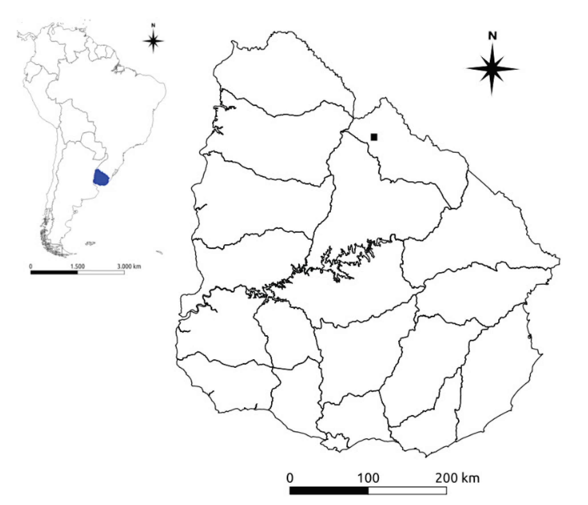
Figure 2.
Localization of specimens within sampled logs.
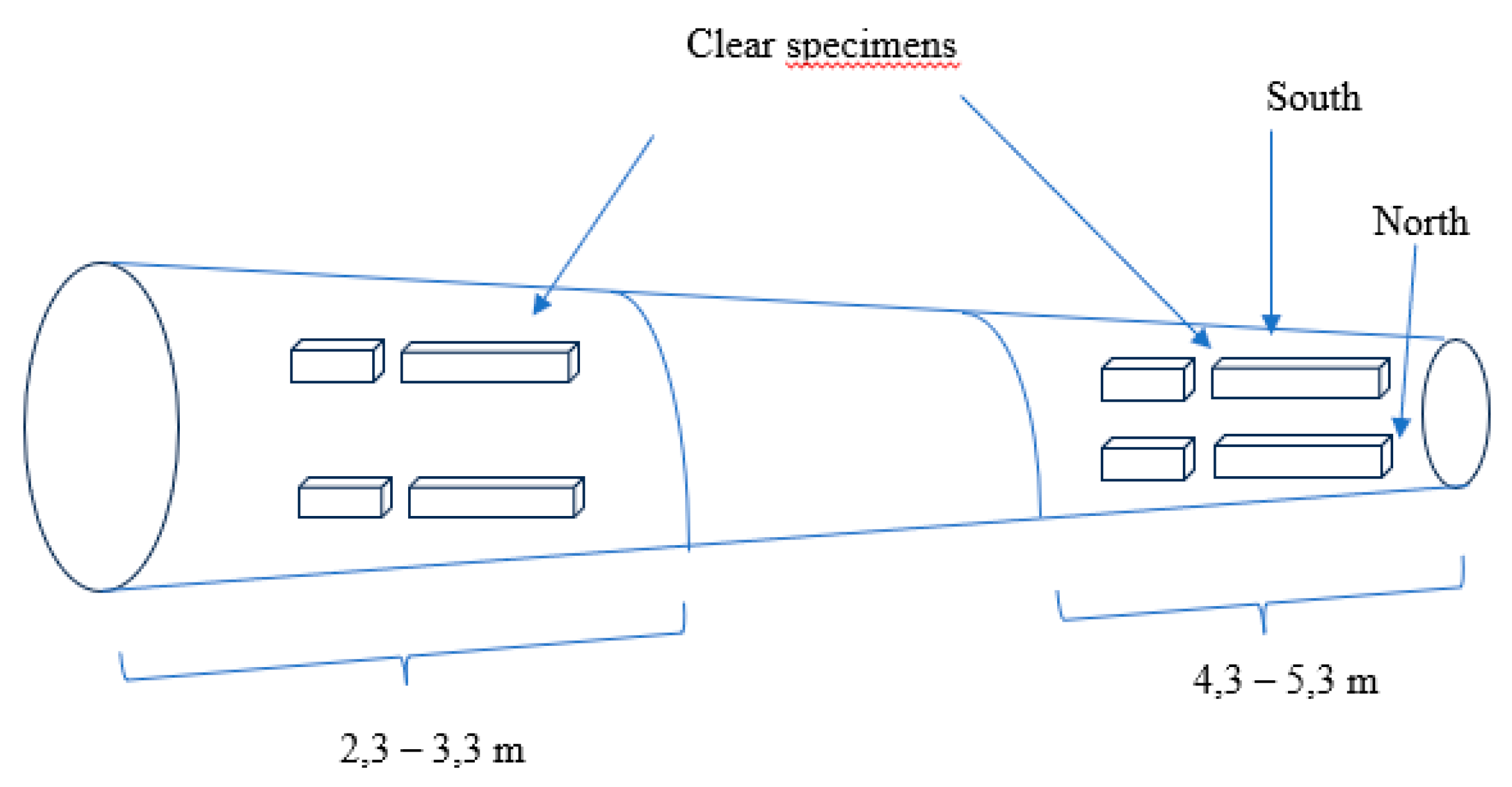
Figure 3.
Growth of mean DBH, CV, Ht and Vi for all thinning regimes evaluated.
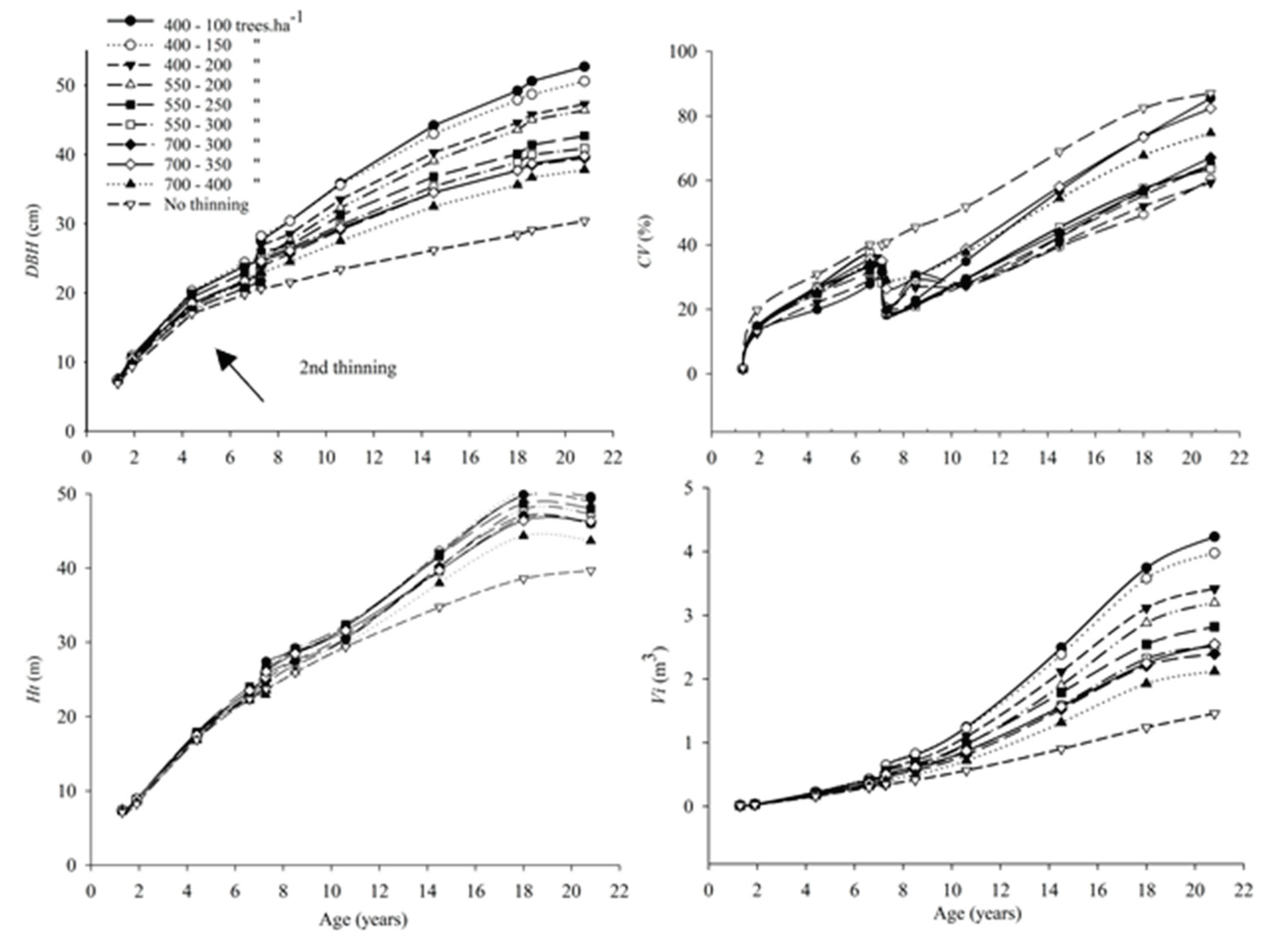
Figure 6.
Mean values of DBH and Vht for the different populations of remaining trees at 20.8 years. Different letters indicate significant differences between thinning schemes at alpha = 0.05 based on a Bonferroni test.
Figure 6.
Mean values of DBH and Vht for the different populations of remaining trees at 20.8 years. Different letters indicate significant differences between thinning schemes at alpha = 0.05 based on a Bonferroni test.
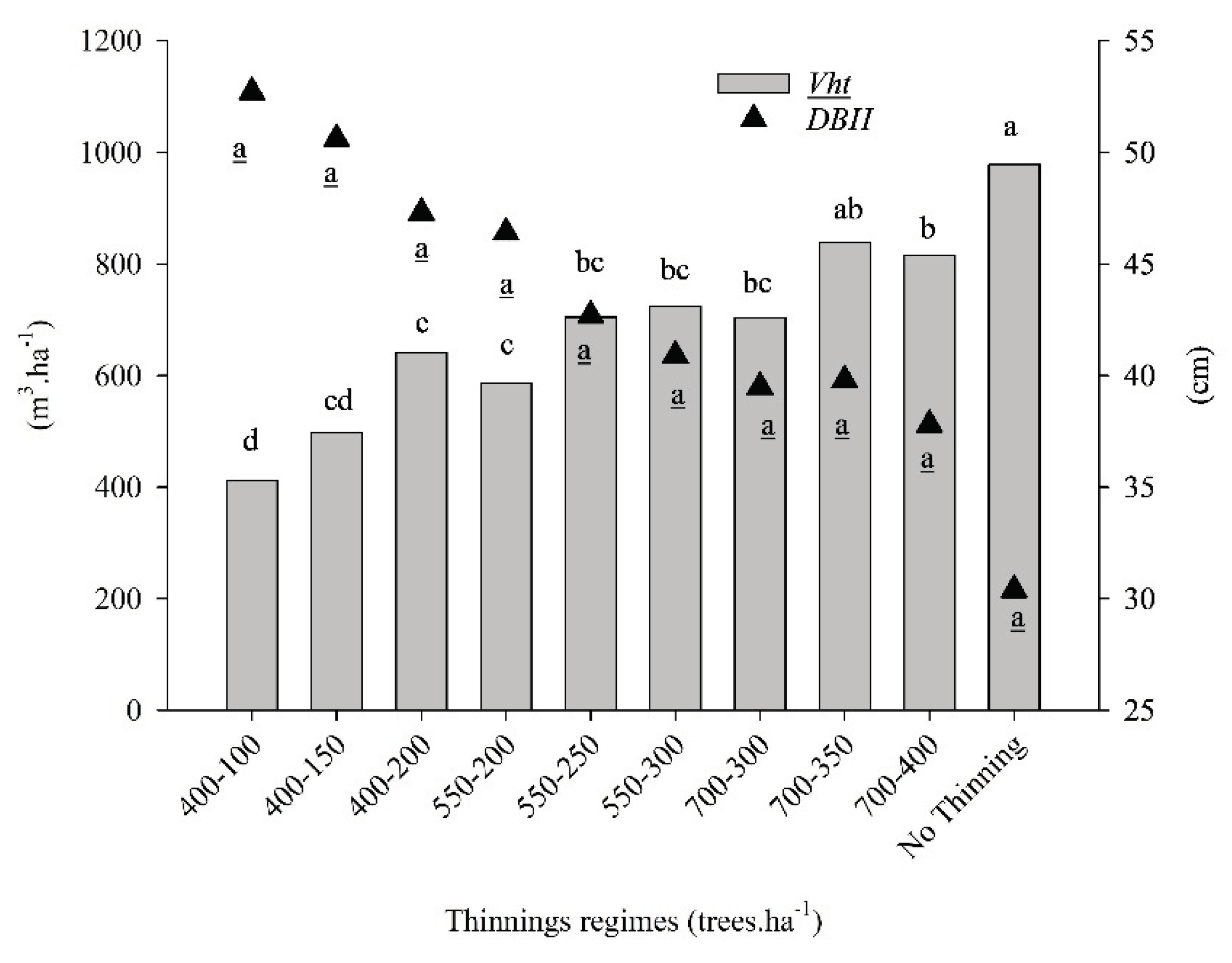
Figure 7.
Bdw and Cd values (5th/95th percentile) of regimes of 400-100, 550-250, and 700-400 trees.ha-1 at the age of 20.8 years. Different letters indicate significant differences between thinning regimes based on a Tukey test (α = 0.05).
Figure 7.
Bdw and Cd values (5th/95th percentile) of regimes of 400-100, 550-250, and 700-400 trees.ha-1 at the age of 20.8 years. Different letters indicate significant differences between thinning regimes based on a Tukey test (α = 0.05).
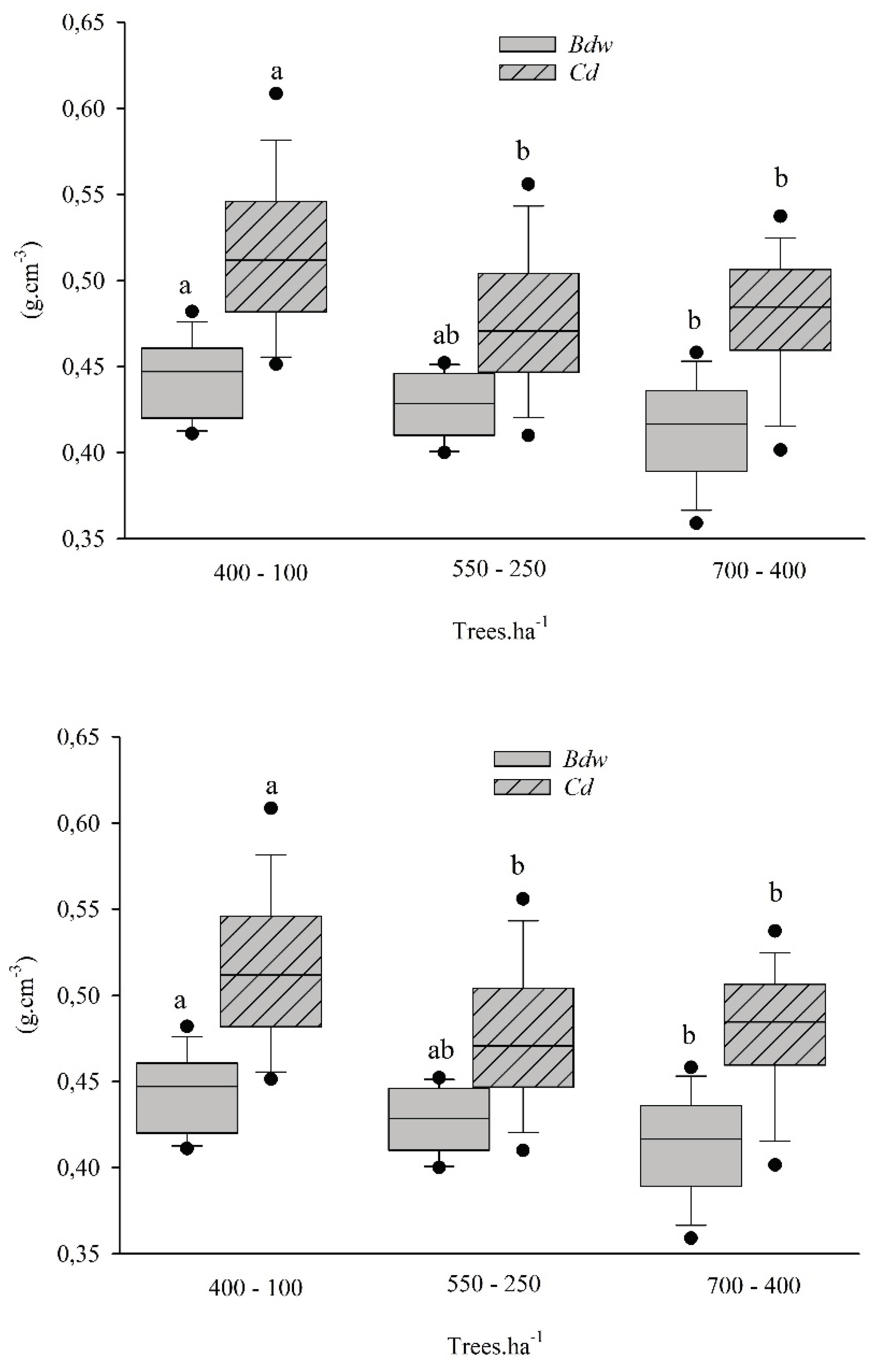
Figure 8.
Comparison of Bdw values (5th /95th percentile) of the thinning regimes 400-100, 550–250, and 700-400 trees.ha-1 at the ages of the second thinning and rotation length.
Figure 8.
Comparison of Bdw values (5th /95th percentile) of the thinning regimes 400-100, 550–250, and 700-400 trees.ha-1 at the ages of the second thinning and rotation length.
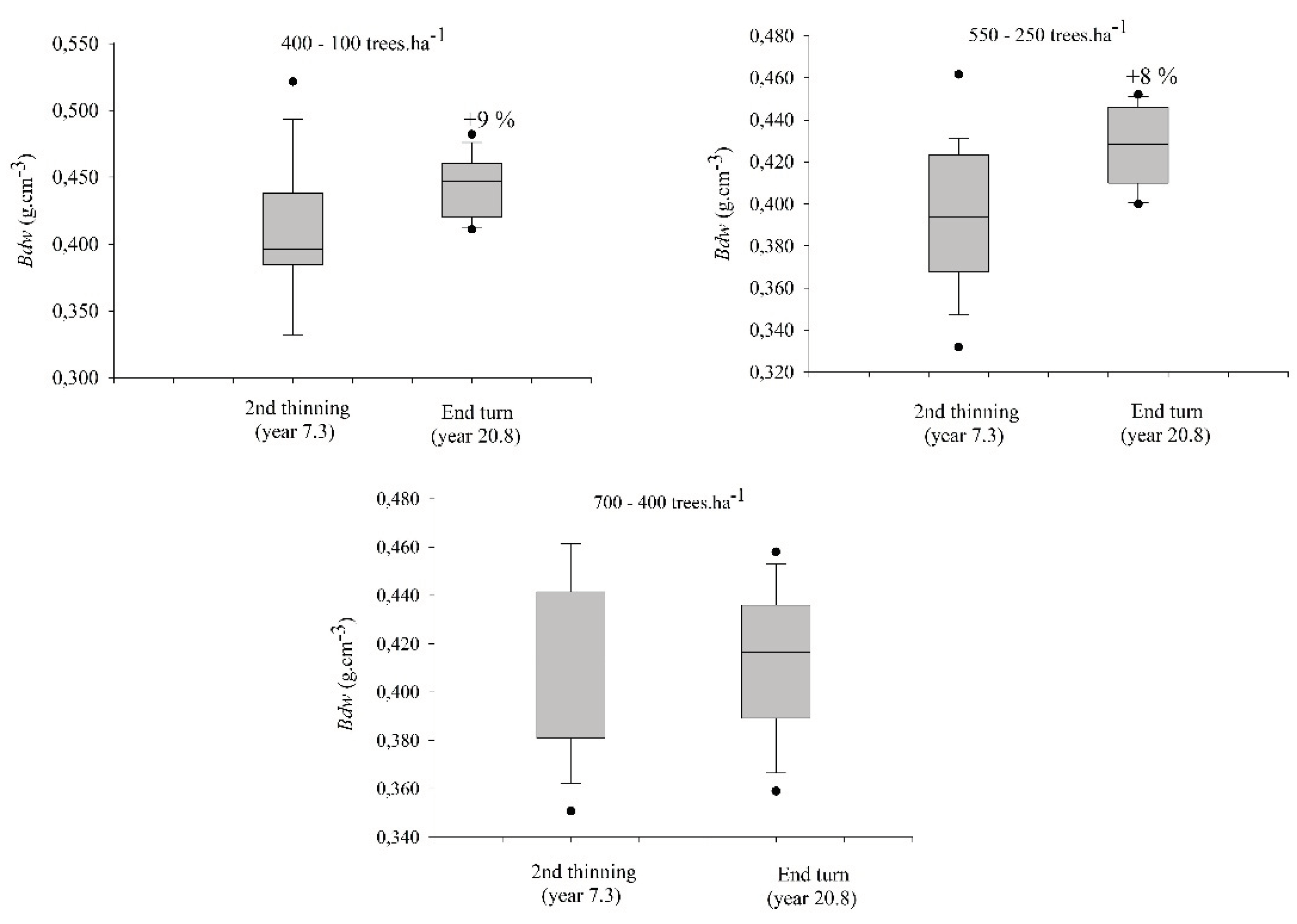
Figure 9.
Comparison of MOEb and MOEc (5th/95th percentile) of the thinning combinations of 400-100, 550-250, and 700-400 trees.ha-1 at the age of 20.8 years. Different letters indicate significant differences between thinning regimes based on a Tukey test (α = 0.05).
Figure 9.
Comparison of MOEb and MOEc (5th/95th percentile) of the thinning combinations of 400-100, 550-250, and 700-400 trees.ha-1 at the age of 20.8 years. Different letters indicate significant differences between thinning regimes based on a Tukey test (α = 0.05).
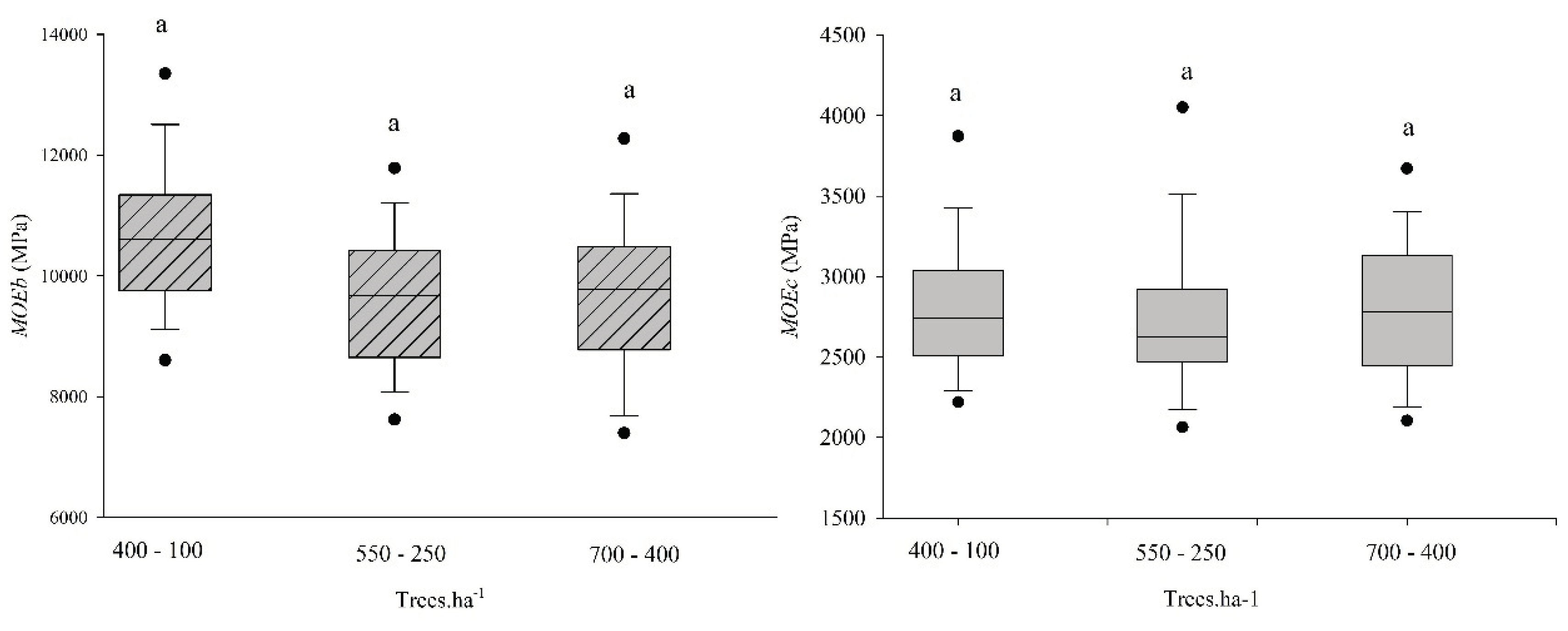
Figure 10.
Comparison of MORf and MORc (5th /95th percentile) of the thinning combinations 400-100, 550-250, and 700-400 trees.ha-1 at the age of 20.8 years. Different letters indicate significant differences between thinning regimes based on a Tukey test (α = 0.05).
Figure 10.
Comparison of MORf and MORc (5th /95th percentile) of the thinning combinations 400-100, 550-250, and 700-400 trees.ha-1 at the age of 20.8 years. Different letters indicate significant differences between thinning regimes based on a Tukey test (α = 0.05).
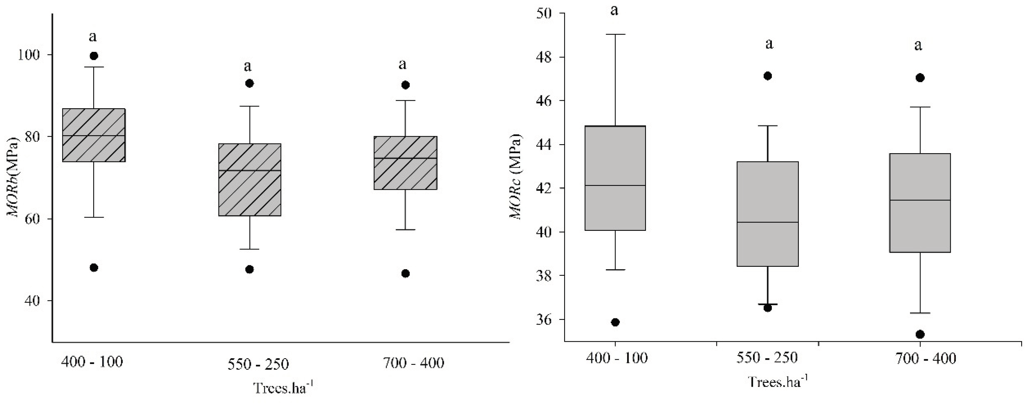

Table 1.
Description of the thinning regime evaluated. Values represent the remanent trees per hectare for each treatment.
Table 1.
Description of the thinning regime evaluated. Values represent the remanent trees per hectare for each treatment.
| First thinning (1.5 years) |
Second thinning (7.3 years) |
Rotation age (20.8 years) |
||
|---|---|---|---|---|
| Prescribed | Effective | Prescribed | Effective | Observed |
| 400 | 372 | 100 | 111 | 97 |
| 400 | 389 | 150 | 142 | 132 |
| 400 | 403 | 200 | 198 | 188 |
| 550 | 545 | 200 | 188 | 188 |
| 550 | 542 | 250 | 250 | 250 |
| 550 | 573 | 300 | 292 | 292 |
| 700 | 677 | 300 | 299 | 299 |
| 700 | 628 | 350 | 347 | 340 |
| 700 | 667 | 400 | 403 | 396 |
| No thinning |
840 | No thinning |
774 | 708 |
Table 2.
Mean values (±SE) of DBH, Ht and Vi for all regimes at 20.8 years. Different letters indicate significant differences based on a Bonferroni test (α = 0.05).
Table 2.
Mean values (±SE) of DBH, Ht and Vi for all regimes at 20.8 years. Different letters indicate significant differences based on a Bonferroni test (α = 0.05).
| Thinning regimes (remaining trees.ha -1) |
DBH (cm) |
Ht (m) |
Vi (m3) |
|---|---|---|---|
| 400-100 | 52.7 (0.3) a | 49.6 (0.6) ab | 4.2 (0.12) a |
| 400-150 | 50.7 (0.7) ab | 50.4 (0.1) a | 4.0 (0.14) ab |
| 400-200 | 47.2 (0.4) b | 48.9 (0.2) ab | 3.4 (0.03) b |
| 550-200 | 46.4 (1.5) bc | 47.2 (0.4) b | 3.2 (0.18) bc |
| 550-250 | 42.7 (0.2) c | 48.0 (1.0) b | 2.8 (0.08) c |
| 550-300 | 40.9 (0.5) cd | 46 (0.5) bc | 2.6 (0.04) cd |
| 700-300 | 39.5 (0.7) cd | 46.1 (0.4) bc | 2.4 (0.12) cd |
| 700-350 | 39.8 (1.0) cd | 46.3 (1.1) bc | 2.5 (0.14) cd |
| 700-400 | 37.8 (0.5) d | 43.7 (1.0) c | 2.1 (0.08) d |
| No thinning | 30.4 (0.7) e | 39.6 (0.8) c | 1.5 (0.05) e |
Table 3.
Mean values (±SE) of Vht extracted and remaining after thinnings. Different letters indicate significant differences between regimes (alpha = 0.05) based on a Bonferroni test.
Table 3.
Mean values (±SE) of Vht extracted and remaining after thinnings. Different letters indicate significant differences between regimes (alpha = 0.05) based on a Bonferroni test.
| Thinning regimes (trees.ha-1) |
2nd Thinning (7.3 years) |
Rotation lenght (20.8 years) |
Total |
|---|---|---|---|
| -------------------(m3 .ha-1)---------------------- | |||
| 400-100 | 113 (2.1) a | 412 (35.3)d | 525 (33.6)d |
| 400-150 | 88 (3.2)b | 498 (35.8) cd | 586 (38.4) cd |
| 400-200 | 75 (3.3) bc | 641 (23.4)c | 716 (26.6)c |
| 550-200 | 97 (4.4) ab | 587 (30.3)c | 684 (34.7)c |
| 550-250 | 103 (5.6) ab | 704 (19.7) bc | 807 (19.9)b |
| 550-300 | 71 (5.9) bc | 724 (15.2) bc | 795 (9.6)b |
| 700-300 | 109 (13.6) ab | 703 (24.3) bc | 812 (19.9)b |
| 700-350 | 77 (8.5) bc | 839 (41.4) ab | 916 (34.7) a |
| 700-400 | 60(5.9)c | 815 (19.7)b | 875 (18.2) ab |
| No thinning | - | 978 (24.0) a | 978 (24.0) a |
Table 4.
RD (considered as a percentage of maximum stand density index) at different ages for all thinning regimes.
Table 4.
RD (considered as a percentage of maximum stand density index) at different ages for all thinning regimes.
| Age (years) | ||||||||||||
|---|---|---|---|---|---|---|---|---|---|---|---|---|
| Thinning regimes (trees.ha-1) | 1.3b | 1.3a | 1.9 | 4.4 | 6.6 | 7.1b | 7.3a | 8.5 | 10.6 | 14.5 | 18 | 20.8 |
| 400-100 | 10 | 9 | 8 | 21 | 28 | 29 | 11 | 12 | 15 | 21 | 24 | 27 |
| 400-150 | 9 | 9 | 8 | 21 | 29 | 30 | 14 | 16 | 19 | 26 | 31 | 34 |
| 400-200 | 9 | 9 | 9 | 23 | 30 | 32 | 18 | 20 | 25 | 33 | 39 | 43 |
| 550-200 | 9 | 9 | 11 | 26 | 34 | 35 | 16 | 19 | 24 | 32 | 38 | 42 |
| 550-250 | 9 | 9 | 11 | 29 | 37 | 39 | 21 | 23 | 29 | 38 | 43 | 48 |
| 550-300 | 10 | 9 | 12 | 28 | 36 | 37 | 23 | 26 | 31 | 41 | 48 | 53 |
| 700-300 | 9 | 9 | 13 | 31 | 40 | 41 | 22 | 25 | 31 | 40 | 47 | 51 |
| 700-350 | 9 | 9 | 13 | 31 | 40 | 42 | 28 | 30 | 36 | 48 | 55 | 61 |
| 700-400 | 0 | 0 | 0 | 30 | 40 | 41 | 29 | 32 | 38 | 50 | 59 | 64 |
| No thinning | 9 | 9 | 15 | 37 | 46 | 48 | 48 | 51 | 58 | 70 | 80 | 84 |
Note: White: Free growth (RD < 30 %) light grey increasing competition (30 % <RD< 55 %, dark grey: fully stocked (RD > 55 %),b: before thinning, a: after thinning.
Table 5.
Vhc for the second thinning and harvest age, categorized by final destination (sawmill and pulp), obtained using a logging simulator for the species.
Table 5.
Vhc for the second thinning and harvest age, categorized by final destination (sawmill and pulp), obtained using a logging simulator for the species.
| Thinning regimes (trees.ha-1) |
2nd Thinning (7.3 years) |
Rotation lenght (20.8 years) |
Total | ||||||
|---|---|---|---|---|---|---|---|---|---|
| Sawmill | pulp | Total | Sawmill | pulp | Total | Sawmill | pulp | Total | |
| --------------------------------------------(m3.ha-1 )--------------------------------------- | |||||||||
| 400-100 | - | 110 | 110 | 310 (88%) |
43 (12%) | 353 | 310 (67%) |
153 (33%) | 463 |
| 400-150 | - | 87 | 87 | 368 (86%) |
59 (14%) | 427 | 368 (72%) |
146 (28%) |
513 |
| 400-200 | - | 72 | 72 | 436 (83%) |
91 (17%) |
527 | 436 (73%) |
163 (27%) |
609 |
| 550-200 | - | 90 | 90 | 414 (82%) |
93 (18%) |
507 | 414 (69%) |
183 (31%) |
597 |
| 550-250 | - | 94 | 94 | 432 (76%) |
135 (24%) |
567 | 432 (65%) |
229 (35%) |
661 |
| 550-300 | - | 71 | 71 | 439 (72%) |
167 (28%) |
606 | 439 (65%) |
238 (35%) |
677 |
| 700-300 | - | 120 | 120 | 386 (69%) |
175 (31%) |
561 | 386 (58%) |
277 (42%) |
663 |
| 700-350 | - | 72 | 72 | 469 (71%) |
196 (29%) |
665 | 469 (64%) |
268 (36%) |
737 |
| 700-400 | - | 56 | 56 | 457 (66%) |
239 (34%) |
696 | 457 (61%) |
295 (39%) |
752 |
| No thinning | - | - | - | 373 (47%) |
413 (53%) |
786 | 373 (47%) |
413 (53%) |
786 |
Table 6.
Simple correlation values of wood density vs. mechanical resistance properties.
| MOEf | MOEc | MORf | MORc | Bdw | Cd | |
|---|---|---|---|---|---|---|
|
Cd p-value |
0.64 < 0.0001 |
0.32* 0.0001 |
0.64 < 0.0001 |
0.63* < 0.0001 |
0.69 < 0.0001 |
- |
|
Bdw p-value |
0.61 < 0.0001 |
0.27 0.12 |
0.44 0.008 |
0.57 0.0003 |
- | - |
*Values calculated with the Spearman test.
Disclaimer/Publisher’s Note: The statements, opinions and data contained in all publications are solely those of the individual author(s) and contributor(s) and not of MDPI and/or the editor(s). MDPI and/or the editor(s) disclaim responsibility for any injury to people or property resulting from any ideas, methods, instructions or products referred to in the content. |
© 2024 by the authors. Licensee MDPI, Basel, Switzerland. This article is an open access article distributed under the terms and conditions of the Creative Commons Attribution (CC BY) license (http://creativecommons.org/licenses/by/4.0/).
Copyright: This open access article is published under a Creative Commons CC BY 4.0 license, which permit the free download, distribution, and reuse, provided that the author and preprint are cited in any reuse.


