
Submitted:
26 March 2024
Posted:
27 March 2024
You are already at the latest version
Abstract
The goal was to model the irrigated (IBY) and rainfed (RBY) bean yields, as a function of essential climatic variables (ECVs), in the center (Culiacán) and south (Rosario) from Sinaloa. In Sinaloa, and for the period 1982–2013 (October–March), the following were calculated: a) temperatures. b) average degree days for the bean, c) cumulative potential evapotranspiration and d) cumulative effective precipitation. For ECVs, from the European Space Agency, e) daily soil moisture. f) IBY and RBY, from the Agrifood and Fisheries Information Service. Multiple linear regressions were applied, which modeled IBY–RBY (dependent variables), as a function of ECVs (independent variables). Then, to establish each Pearson correlation (PC) as significantly different from zero, a hypothesis test was applied: PC vs Pearson's critical correlation (CPC). The four models obtained were significantly predictive: IBY–Culiacán (PC = 0.590 > CPC = |0.349|), RBY–Culiacán (PC = 0.734 > CPC = |0.349|), IBY–Rosario (PC = 0.621 > CPC = |0.355|) and RBY–Rosario (PC = 0.532 > CPC = |0.349|). This study is the first in Sinaloa to predict IBY and RBY based on ECVs, contributing to the production of sustainable food.
Keywords:
significantly different from zero
; multiple linear regressions
; sustainable foods
; the breadbasket of Mexico
1. Introduction
By the year 2050, the world population will increase to approximately 9,725 million inhabitants [1], so, by this same year, food production must also increase by about 70% [2] cited by [3]. Due to these projections, the general assembly of the United Nations [4] adopted the 2030 agenda–sustainable development [5]. This agenda proposes 17 priority goals [5], where the topic “food production” resides in five of this 17 goals: 1) end of poverty, 2) zero hunger, 3) decent work and growth economic, 4) sustainable cities and communities and 5) responsible production and consumption. According to [6,7,8,9,10,11,12,13,14,15], to achieve these five goals, considering the effects of climate change, an efficient tool is the prediction of agricultural crop yield, through multiple linear regressions (MLR) and essential climate variables (ECV). There are 55 ECVs [16], and they stand out for their ease of obtaining and importance in agriculture: 1) average soil moisture (ASM), 2) cumulative effective precipitation (CEP) and air temperature [17,18]. According to [19,20], from the air temperature it is possible to calculate: 3) average maximum temperature (AMT), 4) maximum maximorum temperature (MMT), 4) average minimum temperature (AmT), 5) minimum minimorum temperature (mmT), 6) average mean temperature (AMeT), 7) maximorum mean temperature (MMeT), 8) degree days and 9) cumulative potential evapotranspiration (CET), these nine ECV being those which mainly affect crop yields. According to [21], the crops most sensitive to extreme ECV conditions in Latin America are: corn, wheat and bean. In Mexico, bean is a crop that requires special conditions of ASM and air temperature, both in irrigation (IBY) as in rainfed (RBY) [17], therefore, strategies must be developed to guarantee a source of proteins, mainly for citizens with extreme poverty [22]. Specifically in Sinaloa, sulfur bean is the most cultivated [23], occupying an important place in the annual demand (120,000 tons), obtained with a harvest of 74,000 hectares (average yield of 1.66 T ha– 1) [24]. Although autumn–winter bean is the most widely cultivated in Sinaloa, there are still no prediction models of IBY–RBY. This condition exacerbates the vulnerability of this crop to extreme ECV events, such as frost [25], hot extremes [26] and CEP irregularity, which are common meteorological phenomena in this state [17,26].
In this study, at two meteorological stations in Sinaloa (Culiacán–center and Rosario–south) and for the period 1982–2013 of the autumn–winter cycle (October–March), the following was carried out:
- a)
- For ECVs, using the National Meteorological Service (SMN)–National Water Commission (CONAGUA) database [27], daily series of precipitation and maximum-minimum temperature were obtained. To obtain reliable, long-term and good quality results [28,29], the SMN–CONAGUA daily series were homogenized using the Standard Normal Homogeneity Test (SNHT) method [30]. With the homogenized series, the mean daily temperature (meanT) was determined. Finally, the annual series of: AMT, MMT, AmT, mmT, AMeT, MMeT, average bean degree days (ABDD) [20], CET and CEP were calculated.
- b)
- From the European Space Agency (ESA)–experimental break-adjusted COMBINED Product (version 07.1) [31] – spatial resolution of 0.25° x 0.25°, daily soil moisture was obtained. These data were obtained for two points near the Culiacán and Rosario stations. ASM was calculated annually.
- c)
- From the Agrifood and Fisheries Information Service (SIAP) [32], the annual series of IBY and RBY were obtained.
Standardized Z normalization was applied to the annual series of all variables. Pearson (PC) and Spearman (SC) correlations were applied, depending on the normality of the series. To know the correlations significantly different from zero [33], a hypothesis test was applied between PC and SC vs. Pearson’s critical correlations (CPC) and Spearman (CSC) [7]. Using MRL, four predictive models of IBY–RBY (dependent variables) were obtained as a function of ECVs (independent variables). The four models were significantly predictive (PC > CPC). All MRL met the assumptions of no autocorrelation [34], linearity and severe non-multicollinearity [35,36,37], homogeneity and normality.
The goal was to model IBY–RBY as a function of ECVs, in central and southern Sinaloa.
This study provides models with predictive sensitivity of IBY–RBY [38], based on extreme ECVs events [39,40,41,42,43,44,45,46]. The results contribute to the prevention of negative effects due to possible decreases in IBY–RBY, helping in the production of sustainable foods [5], in a purely agricultural state, considered to this day as “the breadbasket of Mexico” [24].
2. Materials and Methods
Study Area
The state of Sinaloa is located to the northwest of Mexico (Figure 1) and has a predominantly semi-arid aridity index [7]. This state, called “the breadbasket of Mexico,” has historically generated high rates of agricultural production. Specifically, bean cultivation occupies a relevant position, mainly due to the planted area and the economic income generated. For example, in 2013, 69,727 hectares of irrigated land and 4,723 hectares of rainfed land were harvested [24].
Essential Climate Variables (ECVs)
Quality control and homogenization of meteorological series
From SMN–CONAGUA: https://smn.conagua.gob.mx/es/climatologia/informacion-climatologica/informacion-estadistica-climatologica [27], daily series of maximumT and minimumT and precipitation were obtained from 70 meteorological stations in Sinaloa. initially, it was decided to consider the stations that presented daily missing data < 5%. This condition was only met by five stations: Culiacán, Santa Cruz de Alaya, Las Tortugas, Rosario and La Concha. The data from these five stations were previously obtained by [7]. Because [29] argue that, to detect long-term climate change, reliably and with good quality, one must work with homogenized series, in this study, the meteorological series were homogenized with the climatol library (https://climatol.eu) [28,47]. This software is based on the Standard Normal Homogeneity Test method (SNHT) [30]. This library also calculated the missing data, using expression 1:
Where is the estimated meteorological data, through the corresponding nearby data, available at each time step and with the weight assigned to each of them. Statistically, the expression is a linear regression, with a reduced major axis (orthogonal regression), in which the line is adjusted, minimizing the distances of the points perpendicular to it [28].
Temperatures: average maximum (AMT), maximum maximorum (MMT), average minimum (AmT), minimum minimorum (mmT), average mean (AMeT) and maximorum mean (MMeT)
By means of the semi-sum of the homogenized maximumT and minimumT, meanT was obtained. In accordance with what was stated by [19,48,49], the monthly averages of: AMT, MMT, AmT, mmT, AMeT and MMeT were calculated.
Average bean degree days (ABDD), cumulative potential evapotranspiration (CET) and cumulative effective precipitation (CEP)
ABDD was calculated with a daily scale and monthly average (expression 2) [20]:
Where ABDD = average bean degree days (°C day–1), = mean daily temperature and = base temperature = 8.3 °C (for Mexican bean varieties) [20].
To obtain monthly CET, the Hargreaves and Samani method was used [50], expressed by Equation (3). This method was applied due to the absence of relative humidity and wind speed data.
Where CET = cumulative potential evapotranspiration (mm month–1), maximumT = maximum temperature (°C month –1), minimumT = minimum temperature (°C month–1), meanT = mean temperature (°C month–1) and = extraterrestrial solar radiation (mm month–1).
Finally, for the monthly determination of CEP, it was decided to apply expressions 4–5 [51], since according to [52], when the study area is mostly flat, such as Culiacán and Rosario (slope < 5 %,), this method is ideal.
Average soil moisture (ASM)
From ESA: https://catalogue.ceda.ac.uk/uuid/0ae6b18caf8a4aeba7359f11b8ad49ae [31], daily global soil moisture data with a spatial resolution of 0.25° x 0.25° were obtained. This database is called: experimental break-adjusted COMBINED Product, Version 07.1 (version 2023). It was created by direct fusion of soil moisture products from scatterometer and radiometer, level 2 [53]. ESA data have been widely used, for example: [18,54,55,56]. From the global daily data, two sites close to the Culiacán and Rosario stations were selected. The coordinates of these two sites were: Culiacán (24°52′30″ N and 107°22′30″ W) and Rosario (23°07′30″ N and 105°52′30″ W). Finally, ASM was calculated annually for these two sites.
Agricultural variables
Irrigated yield (IBY) and rainfed (RBY) bean for the autumn-winter cycle
From SIAP: http://infosiap.siap.gob.mx/gobmx/datosAbiertos.php [32], a detailed review of the availability of annual IBY–RBY data was carried out. Only two municipalities (Culiacán and Rosario) presented 0 % missing data for the autumn-winter cycle. For IBY–RBY, historically the sowing date ranges from October 15 to November 20, and because, according to SAGARPA–SIAP [57], the sowing–harvest cycle should concentrate ≥ 110 days, the harvest date ranges from February 2 to March 10, approximately.
In this study, the sowing-harvest cycle ranged from October 1 to March 31. Only the period 2003–2013 recorded information divided by municipalities, that is, IBY–RBY for the period 1982–2002, it was at the state level.
The data studied for ECV and IBY–RBY were for the period October–March 1982–2013.
Due to the availability of complete series of ECVs and IBY–RBY, in this study it was decided to work with only two municipalities: Culiacán and Rosario.
Table 1 presents the main statistics for IBY–RBY and ECVs, for the period January–December 1982–2013, at the Culiacán and Rosario stations.
Mathematical Equations that Govern the Statistical Analyses, Applied to Agricultural Variables and Essential Climatic Variables (ECVs)
Normalization
A standardized Z normalization [58] was applied to all series (Equation (6)):
Where = value of the variable of the treated series, = arithmetic mean of the series and = standard deviation of the series.
Normality tests
Shapiro Wilk Method
Four normality tests were applied to all series ( and and residuals). The first test was Shapiro-Wilk [59], which was calculated using expression 7:
Where is the ordered sample of the standardized data with constants.
Anderson–Darling method
The second normality test was Anderson–Darling [60], which is defined by expressions 8–9:
Where is the number of observations, and is defined by expression 9:
Where is the normal cumulative probability distribution function, with mean and variance specified from the sample, and is the data obtained in the sample, ordered from highest to lowest.
Lilliefors Method
Also, the Lilliefors test [61] was applied, where the average and variance of each series were first estimated (expression 10).
Where is the sampling distribution function, is the theoretical distribution function and .
Jarque–Bera method
Finally, the Jarque–Bera test [62] (expression 11) was applied, where the skewness and Kurtosis were used (expressions 12–13).
Where is the sample size, and S and K are respectively the skewness and kurtosis coefficients, which are defined below:
Where is the third moment, around the mean , and is the variance.
Where is the fourth moment, around the mean , and is the variance.
Correlations
Pearson (PC)
When the series presented normality, PC was applied [63], which is based on expression 14.
Where PC = Pearson correlation coefficient, = covariance of and and = standard deviations of and .
Spearman (SC)
SC was used as a second alternative, that is when the series did not follow a normal distribution [63] (expression 15).
Where SC is the Spearman correlation coefficient, is the number of data points in the series, and is the rank difference of element .
Hypothesis tests
To find out if PC and SC were significantly different from zero [7], a hypothesis test was carried out (Equations (16) and (17)). PC and SC were contrasted vs CPC ) and CSC (). CPC and CSC were obtained from [33].
Multiple Linear Regressions (MLR)
Four MLR were carried out: two for Culiacán (irrigated and rainfed) and two for Rosario (irrigated and rainfed). IBY–RBY depended on ECVs: ASM, AMT, MMT, AmT, mmT, AMeT, MMeT, ABDD, CET and CEP. MLR were expressed with Equation (18).
The estimated response, was characterized with sampling regression 19:
Where each regression coefficient was estimated with , from the sample data, using the least squares method. The least squares estimators of the parameters , were obtained by fitting the MLR model (Equation (18)), to the data of expression 20:
Where is the observed response to the values of the independent variables . Each observation (), satisfied Equation (21):
Or each observation (), satisfied expression 22:
Where and are the random error and the residual, respectively, which were associated with the response and with the fitted value [64].
Validation of mathematical models
In the four MLR, the following was done:
- 1)
- 2)
- Goodness-of-fit statistics were calculated: R2, PC, mean error (ME), root mean square error (RMSE), mean error absolute (MEA), percentage of error mean (PEM), percentage of error absolute mean (PEAM) and Theil’s U2 statistic (U2). To comply with the linearity hypothesis, in each MLR, the condition PC ≥ CCP ∴ CP ≠ 0 was met [7].
- 3)
- For the analysis of severe non-multicollinearity, the variance inflation factor (VIF) and tolerance (To) were initially calculated. For severe non-multicollinearity, it was verified that R2 ≤ 0.800, VIF ≤ 5.000 ∴ To > 0.200 [67] cited by [68,69]. In models, the variables that presented severe multicollinearity were eliminated, to subsequently recalculate each MLR.
- 4)
- For the homogeneity, it was verified that the average of each residual serie was zero [70].
- 5)
- Finally, a normality analysis was applied to the residuals of each MLR. Normality methods were the same as for PC and SC.
Software used and statistical significance
In this study, the follow softwares were used: XLstat version 2023, RStudio version 4.3.0, DrinC version 1.7, Past version 4.08, Gretl 2023b, Panoply version 5.2.6, Surfer version 10.0 and CorelDRAW version 2019.
All statistical analyzes were carried out with = 0.05.
3. Results
Agricultural variables and essential climate variables ()
In Culiacán (1992, 1995, 1998–1999 and 2010; Figure 2a,b) and in Rosario (1988, 1995 and 2010–2011; Figure 2c,d), CEP = 0 mm yr–1 was recorded. In 1991, the lowest magnitudes of CET were recorded in Culiacán (CET = 624.338 mm yr–1) and in Rosario (CET = 672.895 mm yr–1).
IBY–Culiacán, ranged from 1.06 t ha–1 in 1987 to 1.98 t ha–1 in 2002 (Figure 2a,b), and IBY–Rosario, varied from 0.90 in 2005 to 1.98 t ha–1 in 2002 (Figure 2c,d). RBY–Culiacán, ranged from 0.42 t ha–1 in 1996 and 2007 to 1.06 t ha–1 in 1982, and RBY–Rosario, varied from 0.42 t ha–1 in 1996 to 1.06 t ha–1 in 1982.
In 1986, the lowest ASM magnitudes were recorded in Culiacán (ASM = 0.020 m3 m–3, Figure 2a), and Rosario (ASM = 0.040 m3 m–3, Figure 2d). The highest magnitudes of ASM were recorded in: 2004 for Culiacán (ASM = 0.194 m3 m–3), in 2005 for Rosario (ASM = 0.232 m3 m–3).
In Culiacán (Figure 2a,b), the highest magnitudes of maximumT were: (AMT = 37.333 °C in 2013, MMT = 36.917 °C in 2005, AMeT = 28.708 °C in 2013, MMeT = 27.417 °C in 2002 and ABDD = 17.643 °C in 2013), and the lowest magnitudes of minimalT were: (AmT = 10.333 °C in 2011 and mmT = 8.583 °C in 1998). In Rosario (Figure 2c,d), the highest magnitudes of maximumT were: (AMT = 35.250 °C in 2013, MMT = 35.417 °C in 1983, AMeT = 26.833 °C in 2013, AMeT = 27.167 °C in 1994 and ABDD = 16.380 °C in 1994), and the lowest magnitudes of minimumT were: (AmT = 10.833 °C in 2011 and mmT = 9.567 °C in 2007).
Correlation
For IBY (Table 2), significant correlations were recorded in IBY–Culiacán vs: AMeT (SC = 0.487), ABDD (SC = 0.486) and ASM (SC = 0.443), and in IBY–Rosario vs: AMeT (SC = 0350). For RBY, significant correlations were recorded in RBY–Culiacán vs: ASM (SC = –0.487) and CEP (SC = 0.375). RBY–Rosario did not register any significant correlation.
Only one case with severe multicollinearity was recorded (AMeT vs ABDD; SC = 0.999, R2 = 0.999). According to [33] and [80], the correlations in bold (Table 2), can be defined as significantly different from zero, since for = 32 (period 1982–2013), a CSC = |0.350| corresponds, that is, SC > CSC.
Models
No ECVs was repeated in all four models (Equations (23)–(26)). Three ECVs were repeated in three models: CEP (IBY–Culiacán, RBY–Culiacán and RBY–Rosario; Equations (23), (24) and (26)), MMT (RBY–Culiacán, RBY–Culiacán and IBY–Rosario; Equations (23)–(25)) and AMT (RBY–Culiacán, IBY–Rosario and RBY–Rosario; Equations (24)–(26)).
–Rosario_1)
Validation
No autocorrelation
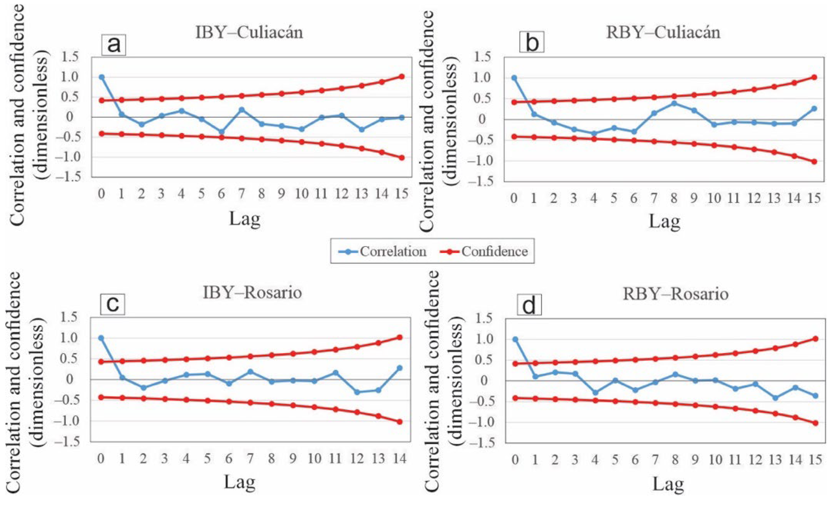
The Breusch–Godfrey contrasts were: IBY–Culiacán (R2 = 0.007, p–value = 0.679 > LMF = 0.175), RBY–Culiacán (R2 = 0.019, p–value = 0.493 > LMF = 0.485), IBY–Rosario (R2 = 0.007, p–value = 0.678 > LMF = 0.177) and RBY–Rosario (R2 = 0.014, p–value = 0.560 > LMF = 0.350). The Ljung–Box contrasts were: IBY–Culiacán (p–value = 0.686 > Q´ = 0.163), RBY–Culiacán (p–value = 0.506 > Q´ = 0.443), IBY–Rosario (p–value = 0.774 > Q´ = 0.083) and RBY–Rosario (p–value = 0.543 > Q´ = 0.369).
Figure 3.
Correlation and confidence of the residuals of the models.
Linearity and severe non-multicollinearity
According to Figure 4 and Table 3, R2 and PC of the models were: IBY–Culiacán (R2 = 0.348, PC = 0.590, n = 32; Figure 4a), RBY–Culiacán (R2 = 0.539, PC = 0.734, n = 32; Figure 4b), IBY–Rosario (R2 = 0.386, PC = 0.621, n = 31; Figure 4c) and RBY–Rosario (R2 = 0.283, PC = 0.532, n = 32; Figure 4c).
Figure 4.
Observed and predicted values of irrigated (IBY) and rainfed (RBY, T ha–1) bean yields, in Culiacán and Rosario. a) IBY–Culiacán, b) RBY–Culiacán, c) IBY–Rosario and d) RBY–Rosario.
Figure 4.
Observed and predicted values of irrigated (IBY) and rainfed (RBY, T ha–1) bean yields, in Culiacán and Rosario. a) IBY–Culiacán, b) RBY–Culiacán, c) IBY–Rosario and d) RBY–Rosario.
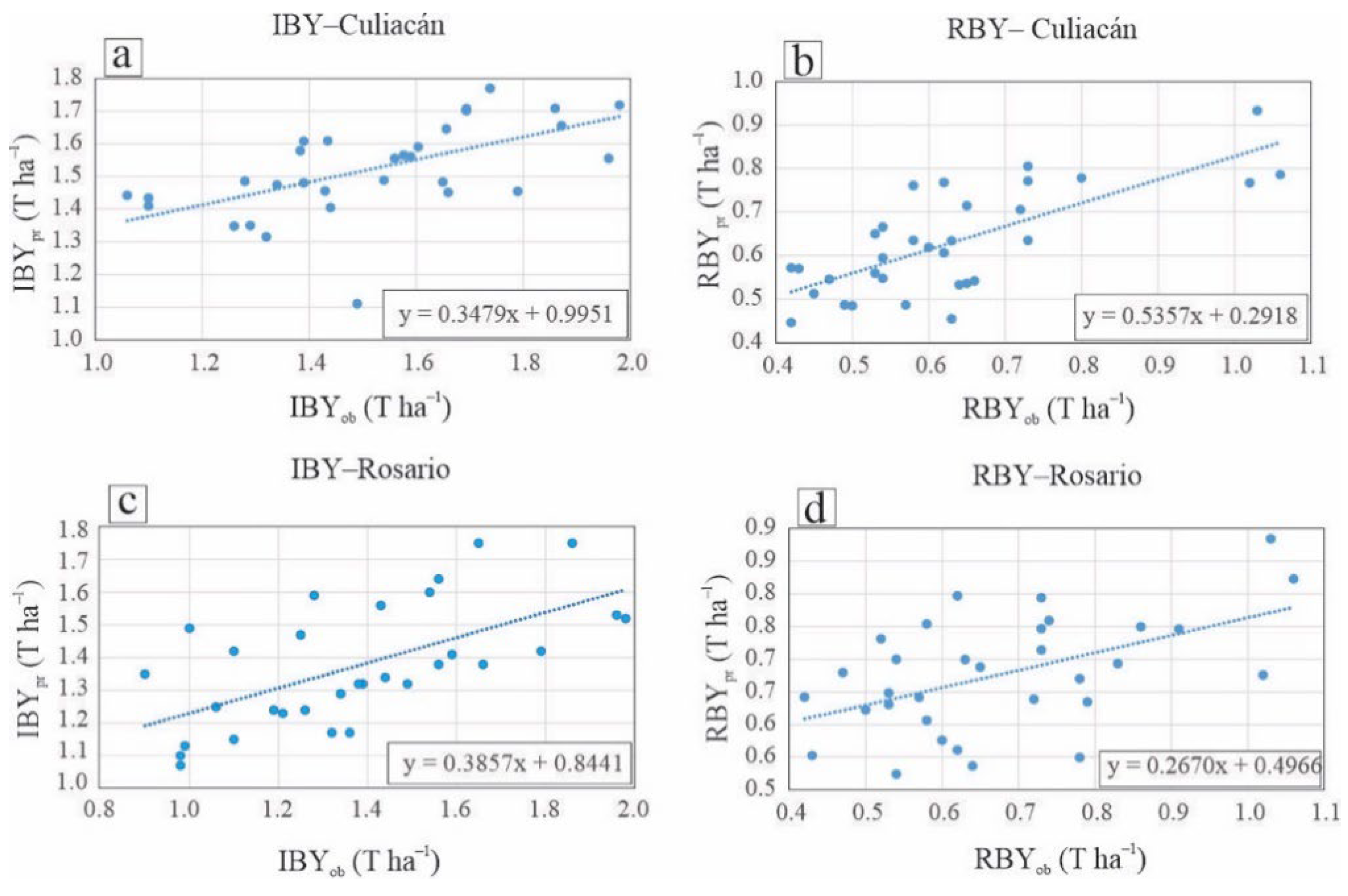
The model with the best fit was RBY–Culiacán: R2 = 0.539, PC = 0.734, ME = 2.255 x 10⁻¹⁶, RMSE = 0.111, MEA = 0.086, PEM = –2.643, PEAM = 13.763 and U2 = 0.743 (Table 3).
In IBY–Culiacán and RBY–Culiacán (Equations (23) and (24)), the variables AMeT and ABDD were not considered, because they were the only ones that presented severe multicollinearity (Table 2).
Homogeneity
The average residue of four models were: IBY–Culiacán (1.250 x 10⁻⁷ T ha–1), RBY–Culiacán (–9.400 x 10⁻⁴ T ha–1), IBY–Rosario (8.618 x 10⁻¹⁸ T ha–1) and RBY–Rosario (0.000 T ha–1).
Normality
In table 4, the p–values of the four normality tests were: IBY–Culiacán (from 0.077 to 0.860), RBY–Culiacán (from 0.070 to 0.344), IBY–Rosario (from 0.890 to 0.963) and RBY–Rosario (from 0.395 to 0.788).

Table 4.
p–values of the normality tests of the residuals of the models.
| P–values of normality tests | ||||
|---|---|---|---|---|
| Dependent variable in each model | Shapiro–Wilk | Anderson–Darling | Lilliefors | Jarque–Bera |
| IBY–Culiacán | 0.410 | 0.211 | 0.077 | 0.860 |
| RBY–Culiacán | 0.158 | 0.185 | 0.070 | 0.344 |
| IBY–Rosario | 0.900 | 0.904 | 0.890 | 0.963 |
| RBY–Rosario | 0.395 | 0.534 | 0.788 | 0.500 |
4. Discussion
The results of CEP and CET (Figure 2a) agree with [71], who point out that, in northern Mexico and for the period 1961–2000, the decade 1990s, they recorded the lowest CEP (from 100 to 900 mm yr–1). The results of IBY–RBY can be attributed to high CEP associated with Hurricane Paul (category 2, occurred in 1982), which elevated RBY–Culiacán and RBY–Rosario [72]. Also, in the periods 1985–1987 and 1996–2003, extreme droughts were recorded in northern Mexico [73,74], which significantly altered IBY–Culiacán. Furthermore, the results of this study are similar to those reported by [75], since these authors point out that, IBY–RBY in Sinaloa and for the autumn-winter cycle of 2021-2022, was 1.93 t ha–1, being fourth place nationally in sown area (85,657 hectares). The results of ASM can be attributed to the fact that, in 1986 (July–September), minimal anomalies occurred: negative ones from the Atlantic multidecadal oscillation and positive ones from the Pacific decadal oscillation, which were generators of La Niña events [76]. Furthermore, according to data from [77] cited by [74], points out that the period 2003–2005 was the one that presented the greatest extreme wet events in northwest Mexico. The results of temperature coincide with those of [25], who point out that, in Culiacán, maximumT increases from 31.600 °C to 34.600 °C, in the period 1982–2008. Figure 2c,d agree with what was stated by [25], since this author points out that 2011 was the most catastrophic year in Sinaloa, due to the lowest historical of minimumT recorded in the last fifty years. These values of minimumT of the autumn-winter cycle caused economic losses of 2,353 million dollars, corresponding to 95% the loss of vegetables and annual crops [78] cited by [79].
According to [33,80], the correlations in bold (Table 2), can be defined as significantly different from zero, since for = 32 (period 1982–2013), a CSC = |0.350| corresponds, that is, SC > CSC. The significant SC can be attributed to the fact that bean are one of the crops most sensitive to maximumT, minimumT, meanT and wet and dry events (ASM and CEP) [20,24,81].
The simultaneous repetition of ECVs (CEP, MMT and AMT) can be attributed to the fact that in IBY–RBY, CEP is essential, generating good availability of ASM [82]. Also, [83] mention that the development of crops in Sinaloa depends largely on the absence of high maximumT, for example, because they could damage the cells and tissues of the bean [20].
According to [84,85], because the condition of p–value > (LMF–Q´) was presented in the four models (Equations (23)–(26)), it can be said that the residuals do not present autocorrelation (Figure 3a–d).
According to [7,33,84], the previous PCs present linearity, since the four MLRs (Figure 4a–d) comply with PC > CPC (CPC = |0.349|, n = 32; CPC = |0.355|, n = 31). Also, all MLRs meet the condition R2 ≤ 0.800, VIF ≤ 5.000 ∴ To > 0.2000 (Table 3), therefore, all models dispense with severe multicollinearity [67] cited by [68].
According to [70], all four models meet the assumption of homogeneity (average residuals = 0).
5. Conclusions
This study is a pioneer in Sinaloa in the prediction of IBY–RBY, using ECVs.
The lower magnitudes of ASM are caused, in large part by the seasonal occurrence (July–September period) of La Niña events (shortage of CEP): minimum negative anomalies of the Atlantic multidecadal oscillation and minimum positive anomalies of the Pacific decadal oscillation. The highest IBY values, are associated with tropical cyclones that have made landfall in Sinaloa, mainly due to their high humidity contributions. In general, ECVs have a greater correlation with IBY than with RBY. IBY–RBY in Culiacán and Rosario, are more sensitive to the extreme values of maximumT indicators, than to minimumT, meanT, ASM, CET and CEP indicators. AMT in Culiacán and Rosario (period 2009–2013), has not stopped increasing, which suggests that IBY–RBY are highly influenced by the occurrence of intense meteorological droughts.
The only event with severe multicollinearity was recorded in Culiacán (AMeT vs ABDD).
The four models met the hypotheses for MLR: no autocorrelation, linearity and severe non-multicollinearity, homogeneity and normality. RBY–Culiacán was the model with the greatest adjustment. IBY–Rosario was the only model to which a delay was applied to its series.
This study provides sensitive tools to prevent damage from a decrease in IBY–RBY, making use of ECVs, which are relatively easy to obtain in Sinaloa, a state that ranks fourth nationally in area planted with beans.
Author Contributions
Conceptualization, Ll.C.O.; methodology, E.G.R.D.; software, P.G.R.E.; validation, Á.D.J.A., G.R.O.G. and T.D.E.; data curation, E.G.R.D.; writing—original draft preparation, Ll.C.O. All authors have read and agreed to the published version of the manuscript.
Funding
This research received no external funding.
Institutional Review Board Statement
Not applicable.
Informed Consent Statement
Not applicable.
Data Availability Statement
https://smn.conagua.gob.mx/es/climatologia/informacion-climatologica/informacion-estadistica-climatologica, https://catalogue.ceda.ac.uk/uuid/0ae6b18caf8a4aeba7359f11b8ad49ae, http://infosiap.siap.gob.mx/gobmx/datosAbiertos.php.
Acknowledgments
To the Research and Postgraduate Secretariat of the National Polytechnic Institute (SIP–IPN) for economic support provided through project SIP20231577.
Conflicts of Interest
The authors declare no conflicts of interest.
References
- United Nations, Department of Economic and Social Affairs, Population Division. World Population Prospects 2022, Online Edition; 2022. https://population.un.org/wpp/Download/Standard/Population/.
- Stacey, N.; Friederike, M.; Hannes, E.; Naomi, S. Economics of Land Degradation Initiative: Report for policy and decision makers_ Reaping economic and environmental benefits from sustainable land management. Bonn, Germany: ELD Initiative and Deutsche Gesellschaft für Internationale Zusammenarbeit (GIZ) GmbH; 2015. https://repo.mel.cgiar.org/handle/20.500.11766/4881.
- Servín, P.M.; Salazar, M.R.; López, C.I.L.; Medina, G.G.; Cid, R.J.A. Predicción de la producción y rendimiento de frijol, con modelos de redes neuronales artificiales y datos climáticos. Biotecnia 2022, 24, 104–111. [CrossRef]
- United Nations (UN). The 2030 Agenda and the Sustainable Development Goals: An opportunity for Latin America and the Caribbean (LC/G.2681-P/Rev.3), Santiago; 2018, 90 p. https://repositorio.cepal.org/server/api/core/bitstreams/6321b2b2-71c3-4c88-b411-32dc215dac3b/content.
- Ballari, D.; Vilches, B.L.M.; Orellana, S.M.L.; Salgado, C.F.; Ochoa, S.A.E.; Graw, V.; Turini, N.; Bendix, J. Satellite Earth Observation for Essential Climate Variables Supporting Sustainable Development Goals: A Review on Applications. Remote Sens. 2023, 15, 2716–2740. [CrossRef]
- Lobell, D.B.; Nicholas, K.C.; Field, C.B. Historical effects of temperature and precipitation on California crop yields. Clim. Change 2007, 81, 187–203. [CrossRef]
- Llanes, C.O.; Norzagaray, C.M.; Gaxiola, A.; Pérez, G.E.; Montiel, M.J.; Troyo, D.E. Sensitivity of Four Indices of Meteorological Drought for Rainfed Maize Yield Prediction in the State of Sinaloa, Mexico. Agriculture 2022, 12, 525–538. [CrossRef]
- Ji, Y.; Chen, Z.; Cheng, Q.; Liu, R.; Li, M.; Yan, X.; Li, G.; Wang, D.; Fu, L.; Ma, Y.; Jin, X.; Zong, X.; Yang, T. Estimation of plant height and yield based on UAV imagery in faba bean (Vicia faba L.). Plant Methods 2022, 18, 26–38. [CrossRef]
- Uspensky, A.B.; Rublev, A.N.; Kozlov, D.A.; Golomolzin, V.V.; Yu., V.; Koslov, I.A.; Nikulin, A.G. Monitoring of the Essential Climate Variables of the Atmosphere. Russ. Meteorol. Hydrol. 2022, 47, 819–828. [CrossRef]
- Wang, S.; Wang, W.; Wu, Y.; Zhao, S. Surface Soil Moisture Inversion and Distribution Based on Spatio-Temporal Fusion of MODIS and Landsat. Sustainability 2022, 14, 9905–9919. [CrossRef]
- Mohammed, A.; Feleke, E. Future climate change impacts on common bean (Phaseolus vulgaris L.) phenology and yield with crop management options in Amhara Region, Ethiopia. CABI A&B 2022, 3, 29–42. [CrossRef]
- Haji, S.B.A.; Sharafati, A.; Motta, D.; Jodar, A.A., Pardo, M.A. Satellite-based prediction of surface dust mass concentration in southeastern Iran using an intelligent approach. Stoch. Env. Res. Risk Assess. 2023, 37, 3731–3745. [CrossRef]
- Qian, C.L.; Shi, W.X.; Jia, Z.; Jia, L.; Yi, Z.; Ze, Z. Ensemble learning prediction of soybean yields in China based on meteorological data. J. Integr. Agric. 2023, 22, 1909–1927. [CrossRef]
- Mohite, J.D.; Sawant, S.A.; Pandit, A.; Agrawal, R.; Pappula, S. Soybean crop yield prediction by integration of remote sensing and weather observations. The International Archives of the Photogrammetry, Remote Sensing and Spatial Information Sciences 2023, Volume XLVIII-M-1-2023. 39th International Symposium on Remote Sensing of Environment (ISRSE-39) “From Human Needs to SDGs”, 24–28 April 2023, Antalya, Türkiye. [CrossRef]
- Zeng, Y.; Su, Z.; Calvet, J.C.; Manninen, T.; Swinnen, E.; Schulz, J.; Roebeling, R.; Poli, P.; Tan, D.; Riihelä, A.; Tanis, C.M.; Arslan, A.N.; Obregon, A.; Kaiser, W.A.; John, V.O.; Timmermans, W.; Timmermans, J.; Kaspar, F.; Gregow, H., Barbu, A.L.; Fairbairn, D.; Gelati, E.; Meurey, C. Analysis of current validation practices in Europe for space-based climate data records of essential climate variables. Int. J. Appl. Earth Obs. Geoinf. 2015, 42, 150–161. [CrossRef]
- Global Climate Observing System (GCOS). Essential Climate Variables. Available online: https://gcos.wmo.int/en/essential-climate-variables (accessed on 22 January 2024).
- Ojeda, B.W. Evaluación del impacto del cambio climático en la productividad de la agricultura de riego y temporal del estado de Sinaloa. Informe final de proyecto, Comisión Nacional de Ciencia y Tecnología (CONACYT), México; 2010, 393 p. http://repositorio.imta.mx/bitstream/handle/20.500.12013/1142/RD_0910_6.pdf?sequence=1&isAllowed=y.
- Liu, Y.; Yang, Y. Advances in the Quality of Global Soil Moisture Products: A Review. Remote Sens. 2022, 14, 3741–3772. [CrossRef]
- Medina, G.G.; Ruiz, C.J.A. Estadísticas climatológicas básicas del estado de Zacatecas. Libro técnico número 3, Instituto Nacional de Investigaciones Forestales, Agrícolas y Pecuarias (INIFAP); 2004, 249 p. http://zacatecas.inifap.gob.mx/publicaciones/climaZacatecas.pdf.
- Barrios, G.E.J.; López, C.C. Temperatura base y tasa de extesnión floliar en frijol. Agrociencia 2009, 43, 29–35. https://www.redalyc.org/pdf/302/30211438004.pdf.
- Carrão, H.; Russo, S.; Sepulcre, C.G.; Barbosa, P. An empirical standardized soil moisture index for agricultural drought assessment from remotely sensed data. Int. J. Appl. Earth Obs. Geoinf. 2016, 48, 74–84. [CrossRef]
- Murillo, A.B.; Troyo, D.E.; García, H.J.L.; Landa, H.L., Larrinaga, M.J.A. El frijol Yorimón: leguminosa tolerante a sequía y salinidad. Editorial Centro de Investigaciones Biológicas del Noroeste; 2000, 33 p. https://cibnor.repositorioinstitucional.mx/jspui/handle/1001/1770.
- Ayala, G.A.V.; Acosta, G.J.A.; Reyes, M.L. El cultivo de frijol: presente y futuro para México. Libro técnico número 1 del Instituto Nacional de Investigaciones Forestales, Agrícolas y Pecuarias (INIFAP); 2021, 236 p. https://vun.inifap.gob.mx/VUN_MEDIA/BibliotecaWeb/_media/_librotecnico/12319_5085_El_cultivo_del_frijol_presente_y_futuro_para_México.pdf.
- Secretaría de Agricultura, Ganadería, Desarrollo Rural, Pesca y Alimentación (SAGARPA). Agenda Técnica Agrícola de Sinaloa, Segunda edición; SAGARPA: México City, Mexico; 2015, 242 p. https://issuu.com/senasica/docs/25_sinaloa_2015_sin.
- Flores, C.L.M.; Arzola, G.J.F.; Ramírez, S.M.; Osorio, P.A. Global climate change impacts in the Sinaloa state, Mexico. Cuadernos de Geografía 2012, 21, 115–119. http://www.scielo.org.co/pdf/rcdg/v21n1/v21n1a09.pdf.
- Llanes, C.O.; Gutiérrez, R.O.G.; Montiel, M.J.; Troyo, D.E. Hot Extremes and Climatological Drought Indicators in the Transitional Semiarid-Subtropical Region of Sinaloa, Northwest Mexico. Pol. J. Environ. Stud. 2022, 31, 4567–4577. [CrossRef]
- Servicio Meteorológico Nacional–Comisión Nacional del Agua (SMN–CONAGUA). Base de datos meteorológicos de México. Available online: https://smn.conagua.gob.mx/es/climatologia/informacion-climatologica/informacion-estadistica-climatologica (accessed on 25 December 2023).
- Guijarro, J.A. Homogenization of Climatological Series with Climatol Version 3.1.1. State Meteorological Agency (AEMET): Balearic Islands, Spain; 2018, 20 p. https://repositorio.aemet.es/bitstream/20.500.11765/12185/2/homog_climatol-en.pdf.
- Argiriou, A.A.; Li, Z.; Armaos, V.; Mamara, A.; Shi, Y.; Yan, Z. Homogenized monthly and daily temperature and precipitation time series in China and Greece since 1960. Adv. Atmos. Sci. 2023, 40, 1326–1336. [CrossRef]
- Alexandersson, H. A homogeneity test applied to precipitation data. J. Climatol. 1986, 6, 661–675. [CrossRef]
- European Space Agency (ESA)–experimental break-adjusted COMBINED Product. Database. Available online: https://data.ceda.ac.uk/neodc/esacci/soil_moisture/data/daily_files/break_adjusted_COMBINED/v07.1 (accessed on 12 August 2023).
- Secretaría de Información Agroalimentaria y Pecuaria (SIAP). Datos abiertos del rendimiento del frijol en México. Available online: http://infosiap.siap.gob.mx/gobmx/datosAbiertos.php (accessed on 25 January 2023).
- Oxford Cambridge and RSA (OCR). Formulae and statistical tables (ST1). 1–8: database of critical values. Available online: https://www.ocr.org.uk/Images/174103-unit-h869-02-statistical-problem-solving-statistical-tables-st1-.pdf (accessed on 15 December 2023).
- Bouza, H.C.N. Modelos de regresión y sus aplicaciones. Reporte técnico; 2018, 124 p. https://www.researchgate.net/profile/Carlosouza/publication/323227561_MODELOS_DE_REGRESION_Y_SUS_APLICACIONES/links/5a871265a6fdcc6b1a3abe40/MODELOS-DE-REGRESION-Y-SUS-APLICACIONES.pdf.
- Liang, L.; Cui, H.; Arabameri, A.; Arora, A.; Danesh, S.A. Landslide susceptibility mapping: application of novel hybridization of rotation forests (RF) and Java decision trees (J48). Soft Comput. 2023, 27, 17387–17402. [CrossRef]
- Jinse, J.; Varadharajan, R. Simultaneous raise regression: a novel approach to combating collinearity in linear regression models. Qual. Quant. 2023, 57, 4365–4386. [CrossRef]
- Akingboye, A.S.; Bery, A.A. Development of novel velocity–resistivity relationships for granitic terrains based on complex collocated geotomographic modeling and supervised statistical analysis. Acta Geophys. 2023, 71, 2675–2698. [CrossRef]
- Romero, F.C.S.; López, C.C.; Kohashi, S.J.; Miranda, C.S.; Aguilar, R.V.H.; Martínez, R.C.G. Cambios en el rendimiento y sus componentes en frijol bajo riego y sequía. Rev. Mexicana Cienc. Agríc. 2019, 10, 351–364. [CrossRef]
- Li, S.; You, S.; Song, Z.; Zhang, L.; Liu, Y. Impacts of Climate and Environmental Change on Bean Cultivation in China. Atmos. 2021, 12, 1591–1606. [CrossRef]
- Mardan, M.; Ahmadi, S. Soil moisture retrieval over agricultural fields through integration of synthetic aperture radar and optical image. Gisci. Remote sens. 2021, 58, 1276–1299. [CrossRef]
- Fu, W.M.C.; Molin, J.P. Soybean Yield Estimation and Its Components: A Linear Regression Approach. Agriculture 2020, 10, 348–360. [CrossRef]
- Chakraborty, A.; Krishnamurti, T.N. Numerical simulation of the North American monsoon system. Meteorol. Atmos. Phys. 2003, 84, 57–82. https://link.springer.com/article/10.1007/s00703-002-0566-6.
- Amador, R.M.D.; Acosta, D.E.; Medina, G.G.; Gutiérrez, L.R. An empirical model to predict yield of rainfed dry bean with multi-year data. Rev. Fitotec. Mex. 2007, 30, 311–319. https://www.redalyc.org/pdf/610/61003014.pdf.
- Medina, G.G.; Baez, G.A.D.; López, H.J.; Ruiz, C.J.A.; Tinoco, A.C.A.; Kiniry, J.R. Large-area dry bean yield prediction modeling in Mexico. Rev. Mexicana Cienc. Agríc. 2010, 1, 407–420. https://www.redalyc.org/pdf/2631/263120630010.pdf.
- Gonzalez, G.M.A.; Guertin, D.P. Seasonal bean yield forecast for non-irrigated croplands through climate and vegetation index data: Geospatial effects. Int. J. Appl. Earth Obs. Geoinf. 2021, 105, 102623–102634. [CrossRef]
- Botero, H.; Barnes, A.P. The effect of ENSO on common bean production in Colombia: a time series approach. Food Secur. 2022, 14, 1417–1430. [CrossRef]
- Guijarro, J.A. Package climatol. R Package Version, 4.0.0; 2023, 40 p.
- Ruiz, C.J.A.; Medina, G.G.; Macías, J.C.; Silva, M.M.S.; Diaz, P.G. Estadísticas climatológicas básicas del estado de Sinaloa (Período 1961- 2003). Libro Técnico Núm. 2. INIFAP-CIRNO. Cd. Obregón, Sonora, México; 2005. https://docplayer.es/41213292-Estadisticas-climatologicas-basicas-del-estado-de-sinaloa-periodo.html.
- Llanes, C.O.; Cervantes, A.L.; González, G.G.E. Calculation of indicators of maximum extreme temperature in Sinaloa state, northwestern Mexico. Earth Sci. Res. J. 2023, 27, 77–84. [CrossRef]
- Hargreaves, G.H.; Samani, Z.A. Reference crop evapotranspiration from temperature. Applied Eng. in Agric. 1985, 1, 96–99. https://www.researchgate.net/publication/247373660_Reference_Crop_Evapotranspiration_From_Temperature.
- Brouwer, C.; Heibloem, M. Irrigation water management: Irrigation water needs. Rome: Food and Agriculture Organization (FAO); 1986. https://www.fao.org/3/s2022e/s2022e07.htm.
- Flores, G.H. Impacto del cambio climático en los distritos de riego de Sinaloa. Tesis de Maestría del Colegio de Postgraduados Campius Montecillo, 2010, 204 p. [CrossRef]
- Dorigo, W.; Preimesberger, W.; Moesinger, L.; Pasik, A.; Scanlon, T.; Hahn, S.; Van der Schalie, R.; Van der Vliet, M., De Jeu, R.; Kidd, R.; Rodriguez, F.N.; Hirschi, M. ESA Soil Moisture Climate Change Initiative (Soil_Moisture_cci): Experimental Break-Adjusted COMBINED Product, Version 07.1. NERC EDS Centre for Environmental Data Analysis; 2023. Available online: https://catalogue.ceda.ac.uk/uuid/0ae6b18caf8a4aeba7359f11b8ad49ae (accessed on 15 December 2023).
- Seo, E.; Dirmeyer, P.A. Improving the ESA CCI daily soil moisture time series with physically based land surface model dataset using a Fourier time-filtering method. J. Hydrometeorol. 2022, 23, 473–489. [CrossRef]
- Feng, S.; Huang, X.; Zhao, S.; Qin, Z.; Fan, J.; Zhao, S. Evaluation of Several Satellite-Based Soil Moisture Products in the Continental US. Sensors 2022, 22, 9977–9994. [CrossRef]
- Yu, W.; Li, Y.; Liu, G. Calibration of the ESA CCI-Combined Soil Moisture Products on the Qinghai-Tibet Plateau. Remote Sens. 2023, 15, 918–932. [CrossRef]
- Secretaría de Agricultura y Desarrollo Rural (SAGARPA) y Servicio de Información Agroalimentaria y Pesquera (SIAP). Aptitud agroaclimática del frijol en México ciclo agrícola otoño–inverno. Informe técnico; 2019, 30 p. https://www.gob.mx/cms/uploads/attachment/file/495087/Reporte_de_Aptitud_agroclim_tica_de_M_xico_del_frijol_OI_2019-2020.pdf.
- Wu, H.; Hayes, J.M.; Weiss, A.; Hu, Q. An evaluation of the standardized precipitation index, the China–Z index and the statistical Z–score. Int. J. Climatol. 2001, 21, 745–758. [CrossRef]
- Shapiro, S.S.; Wilk, M.B. An analysis of variance test for normality (complete samples). Biometrika 1965, 52, 591–611. https://www.bios.unc.edu/~mhudgens/bios/662/2008fall/Backup/wilkshapiro1965.pdf.
- Anderson, T.W.; Darling, D.A. A test of goodness of fit. J. Amer. Stat. Assn. 1954, 49, 765–769. [CrossRef]
- Lilliefors, H. On the Kolmogorov-Smirnov test for normality with mean and variance unknown‖. J. Amer. Statist. Assoc. 1967, 62, 399–402. http://www.bios.unc.edu/~mhudgens/bios/662/2008fall/Backup/lilliefors1967.pdf.
- Jarque, M.C.; Bera, K.A. A test for normality of observations and regression residual. Int. Stat. Rev. 1987, 55, 163–172. http://webspace.ship.edu/pgmarr/Geo441/Readings/Jarque%20and%20Bera%201987%20-%20A%20Test%20for%20Normality%20of%20Observations%20and%20Regression%20Residuals.pdf.
- Hauke, J.; Kossowski, T. Comparison of values of Pearson’s and Spearman’s correlation coefficients on the same sets of data. Quaest. Geogr. 2011, 30, 87–93. https://www.researchgate.net/publication/227640806_Comparison_of_Values_of_Pearson%27s_and_Spearman%27s_Correlation_Coefficients_on_the_Same_Sets_of_Data.
- Walpole, E.R.; Myers, H.R.; Myers, L.S.; Ye, K. Probabilidad y estadística para ingeniería y ciencias. Universidad de Texas, San Antonio, editorial Pearson; 2012, 816 p. https://vereniciafunez94hotmail.files.wordpress.com/2014/08/8va-probabilidad-y-estadistica-para-ingenier-walpole_8.pdf.
- Breusch, T.S. "Testing for Autocorrelation in Dynamic Linear Models. Aust. Econ. Pap. 1978, 17, 334–355. [CrossRef]
- Ljung, G.M.; Box, G.E.P. On a measure of lack of fit in time series models. Biométrika 1978, 65, 297–303. [CrossRef]
- Kleinbaum, D.G.; Kupper, L.L.; Muller, K.E. Applied regression analysis and other multivariable methods. PWS-Kent, Boston; 1988. https://ebin.pub/applied-regression-analysis-and-other-multivariable-methods-5nbsped-1285051084-9781285051086.html.
- Deduy, G.I. Regresión sobre componentes principals. Tesis de Licenciatura, Universidad de Sevilla. Available online: https://idus.us.es/bitstream/handle/11441/90005/Deduy%20Guerra%20Irene%20TFG.pdf?sequence=1&isAllowed=y (accessed on 20 December 2023).
- Kutner, H.M.; Nachtsheim, J.C.; Neter, J.; Li, W. Applied linear statistical models (fifth edition). Editorial McGraw–Hill Irwin; 2005, 1415 p. https://users.stat.ufl.edu/~winner/sta4211/ALSM_5Ed_Kutner.pdf.
- Carrasquilla, B.A.; Chacón, R.A.; Núñez, M.K., Gómez, E.O.; Valverde, J.; Guerrero, B.M. Regresión lineal simple y múltiple: aplicación en la predicción de variables naturales relacionadas con el crecimiento microalgal. Tecnología en Marcha. Encuentro de Investigación y Extensión; 2016, 33-45. https://www.scielo.sa.cr/scielo.php?pid=S0379-39822016000900033&script=sci_abstract&tlng=es.
- Llanes, C.O.; Norzagaray, C.M.; Gaxiola, A.; González, G.G.E. Regional precipitation teleconnected with PDO–AMO–ENSO in northern Mexico. Theor. Appl. Climatol. 2020, 140, 667–681. [CrossRef]
- Servicio Meteorológico Nacional (SMN). Ciclones que han impactado en México, 1981–2001. Cuadro I.8.1.; 2002. https://paot.org.mx/centro/ine-semarnat/informe02/estadisticas_2000/compendio_2000/01dim_social/01_08_Desastres/data_desastres/CuadroI.8.1b.htm.
- Méndez, M., Magaña, V. Regional Aspects of Prolonged Meteorological Droughts over Mexico and Central American. J. Clim. 2010, 5, 1175–1188. [CrossRef]
- Llanes, C.O.; Gaxiola, H.A.; Estrella, G.R.D.; Norzagaray, C.M.; Troyo, D.E.; Pérez, G.E.; Ruiz, G.R.; Pellegrini, C.M.J. Variability and Factors of Influence of Extreme Wet and Dry Events in Northern Mexico. Atmos. 2018, 9, 12–27. [CrossRef]
- Avila, M.J.A.; Ávila, S.J.M.; Rivas, S.F.J.; Martínez, H.D. El Cultivo del frijol: Sistemas de producción en el noroeste de México. Universidad de Sonora; 2023, 88 p. https://agricultura.unison.mx/memorias%20de%20maestros/EL%20CULTIVO%20DEL%20FRIJOL.pdf.
- Llanes, C.O. Predictive association between meteorological drought and climate indices in the state of Sinaloa, northwestern Mexico. Arab. J. Geosci. 2023, 16, 1–14. [CrossRef]
- Comisión Nacional del Agua (CONAGUA). Base de Datos del Índice Estandarizado de Precipitación (SPI). Secretaría de Gobernación de México. Available online: https://smn.conagua.gob.mx/es/climatologia/monitor-de-sequia/spi. (accessed on 22 october 2023).
- Soria, R.J.; Fernández, O.Y.; Quijano, C.A.; Macías, C.J.; Sauceda, P.; González, D.; Quintana, J. Remote sensing and simulation models for crop management. Proceedings of progress in electromagnetics research symposium. Moscow, Russia; 2012. https://www.researchgate.net/publication/289288401_Remote_sensing_and_simulation_model_for_crop_management.
- Jasso, M.M.; Soria, R.J.; Antonio, N.X. Pérdida de superficies cultivadas de maíz de temporal por efecto de heladas en el valle de Toluca. Rev. Mexicana Cienc. Agríc. 2022, 13, 207–222. [CrossRef]
- Schober, P.; Boer, C.; Schwarte, L.A. Correlation Coefficients: Appropriate Use and Interpretation. Anesth. Analg. 2018, 126, 1763–1768. DOI: 10.1213/ANE.0000000000002864.
- Zhenhua, L.; Ziqing, X.; Feixiang, C.; Yueming, H.; Ya, W.; Jianbin, L.; Huiming, L.; Luo, L. Soil Moisture Index Model for Retrieving soil Moisture in Semiarid Regions of China. IEEE J. Sel. Top. Appl. Earth Obs. Remote Sens. 2020, 13, 5929–5937. https://ieeexplore.ieee.org/stamp/stamp.jsp?arnumber=9204441.
- Rosales, S.R.; Ochoa, M.R.; Acosta, G.J.A. Fenología y rendimiento del frijol en el altiplano de México y su respuesta al Fotoperiodo. Agrociencia 2001, 35, 513–523. https://www.redalyc.org/pdf/302/30235505.pdf.
- Sifuentes, E.; Macías, J.; Ojeda, W.; González, V.M.; Salinas, D.A., Quintana, J.G. Gestión de riego enfocada a variabilidad climática en el cultivo de papa: aplicación al distrito de riego 075, Río fuerte, Sinaloa, México. Tecnol. Cienc. Agua 2016, 7, 149–168. https://www.scielo.org.mx/pdf/tca/v7n2/2007-2422-tca-7-02-00149.pdf.
- Morantes, Q.G.R.; Rincón, P.G.; Pérez, S.N.A. Modelo de regresión lineal múltiple para estimar concentración de PM1. Rev. Int. Contam. Ambie. 2019, 35, 179–194. https://www.revistascca.unam.mx/rica/index.php/rica/article/view/RICA.2019.35.01.13.
- Pérez, R.; López, A.J. Econometría aplicada con Gretl. Universidad de Oviedo; 2019, 385 p. https://www.researchgate.net/profile/Ana-Lopez-Menendez/publication/334771581_Econometria_Aplicada_con_Gretl/links/5d40766ba6fdcc370a6eedb8/Econometria-Aplicada-con-Gretl.pdf.
Figure 1.
Study area. Location of the meteorological stations in the center (Culiacán) and south (Rosario) of the state of Sinaloa, Mexico.
Figure 1.
Study area. Location of the meteorological stations in the center (Culiacán) and south (Rosario) of the state of Sinaloa, Mexico.
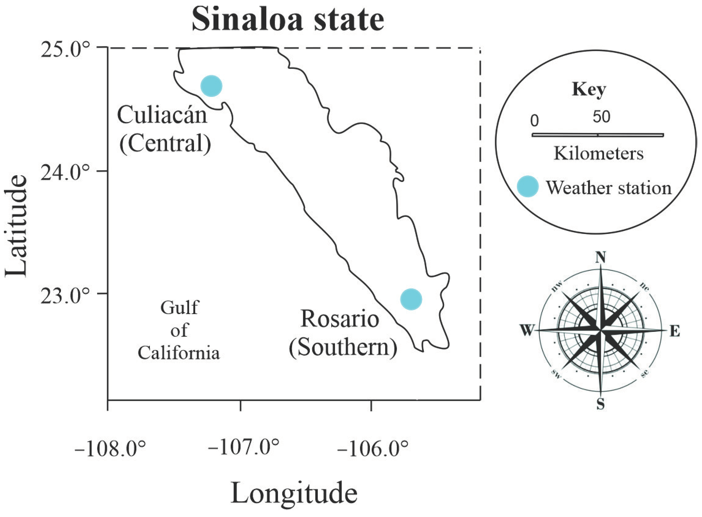
Figure 2.
Irrigated (IBY) and rainfed (RBY) beans yields, and essential climatic variables (ECVs), for Culiacán and Rosario. a) and c) variables without normalization, and b) and d) variables with normalization.
Figure 2.
Irrigated (IBY) and rainfed (RBY) beans yields, and essential climatic variables (ECVs), for Culiacán and Rosario. a) and c) variables without normalization, and b) and d) variables with normalization.

Table 1.
Main annual statistics in the period January–December 1982–2013, for the irrigated (IBY) and rainfed (RBY) bean yield and essential climate variables (ECVs) in central and southern Sinaloa.
Table 1.
Main annual statistics in the period January–December 1982–2013, for the irrigated (IBY) and rainfed (RBY) bean yield and essential climate variables (ECVs) in central and southern Sinaloa.
| Variable | Statistical variable | Culiacán | Rosario | Variable | Statistical variable | Culiacán | Rosario |
|---|---|---|---|---|---|---|---|
| IBY | Average (T ha–1) | 1.526 | 1.372 | mmT | Average (T ha–1) | 14.497 | 15.083 |
| Standard deviation (T ha–1) | 0.242 | 0.291 | Standard deviation (T ha–1) | 5.806 | 5.247 | ||
| Variance (T ha–1)2 | 0.059 | 0.085 | Variance (T ha–1)2 | 33.699 | 27.527 | ||
| Coefficient of variation (%) | 15.867 | 21.207 | Coefficient of variation (%) | 40.044 | 34.784 | ||
| RBY | Average (T ha–1) | 0.628 | 0.678 | AMeT | Average (T ha–1) | 25.785 | 25.634 |
| Standard deviation (T ha–1) | 0.165 | 0.171 | Standard deviation (T ha–1) | 4.137 | 3.091 | ||
| Variance (T ha–1)2 | 0.027 | 0.029 | Variance (T ha–1)2 | 17.116 | 9.552 | ||
| Coefficient of variation (%) | 26.231 | 25.178 | Coefficient of variation (%) | 16.045 | 12.057 | ||
| ASM | Average (T ha–1) | 0.126 | 0.155 | MMeT | Average (T ha–1) | 28.706 | 28.166 |
| Standard deviation (T ha–1) | 0.051 | 0.061 | Standard deviation (T ha–1) | 3.857 | 2.892 | ||
| Variance (T ha–1)2 | 0.003 | 0.004 | Variance (T ha–1)2 | 14.874 | 8.363 | ||
| Coefficient of variation (%) | 40.344 | 39.305 | Coefficient of variation (%) | 13.435 | 10.267 | ||
| AMT | Average (T ha–1) | 33.260 | 32.490 | ABDD | Average (T ha–1) | 17.485 | 17.334 |
| Standard deviation (T ha–1) | 3.332 | 2.232 | Standard deviation (T ha–1) | 4.137 | 3.091 | ||
| Variance (T ha–1)2 | 11.102 | 4.981 | Variance (T ha–1)2 | 17.116 | 9.552 | ||
| Coefficient of variation (%) | 10.018 | 6.869 | Coefficient of variation (%) | 23.661 | 17.831 | ||
| MMT | Average (T ha–1) | 37.184 | 35.593 | CET | Average (T ha–1) | 1834.742 | 1799.484 |
| Standard deviation (T ha–1) | 2.967 | 2.101 | Standard deviation (T ha–1) | 41.421 | 58.663 | ||
| Variance (T ha–1)2 | 8.802 | 4.414 | Variance (T ha–1)2 | 1715.697 | 3441.351 | ||
| Coefficient of variation (%) | 7.979 | 5.903 | Coefficient of variation (%) | 2.258 | 3.260 | ||
| AmT | Average (T ha–1) | 18.310 | 18.778 | CEP | Average (T ha–1) | 416.862 | 578.381 |
| Standard deviation (T ha–1) | 5.199 | 4.597 | Standard deviation (T ha–1) | 102.271 | 138.621 | ||
| Variance (T ha–1)2 | 27.026 | 21.135 | Variance (T ha–1)2 | 10459.329 | 19215.710 | ||
| Coefficient of variation (%) | 28.393 | 24.482 | Coefficient of variation (%) | 24.534 | 23.967 |
Table 2.
Pearson (PC) and Spearman (SC) correlation coefficients between the irrigated (IBY) and rainfed (RBY) bean yields, and the essential climatic variables (ECVs) in Sinaloa.
Table 2.
Pearson (PC) and Spearman (SC) correlation coefficients between the irrigated (IBY) and rainfed (RBY) bean yields, and the essential climatic variables (ECVs) in Sinaloa.
| Variable | IBY (T Ha–1 yr–1) |
RBY (T Ha–1 yr–1) |
ASM (m3 m–3 yr–1) |
AMT (°C yr–1) |
MMT (°C) |
AmT (°C yr–1) |
mmT (°C) |
AMeT (°C yr–1) |
MMeT (°C) |
ABDD (°C yr–1) |
CET (mm yr–1) |
CEP (mm yr–1) |
|
|---|---|---|---|---|---|---|---|---|---|---|---|---|---|
| Culiacán | IBY (T Ha–1 yr–1) | 0.939 | 0.005 | 0.178 | 0.966 | 0.640 | 0.299 | 0.014 | 0.521 | 0.039 | 0.367 | 0.301 | |
| RBY (T Ha–1 yr-1) | 0.135 | 0.001 | 0.850 | 0.609 | 0.515 | 0.885 | 0.694 | 0.726 | 0.722 | 0.653 | 0.096 | ||
| ASM (m3 m–3 yr–1) | 0.443 | –0.487 | 0.056 | 0.062 | 0.402 | 0.371 | 0.016 | 0.158 | 0.094 | 0.286 | 0.193 | ||
| AMT (°C yr–1) | 0.260 | –0.071 | 0.435 | 0.834 | 0.377 | 0.235 | 0.000 | 0.667 | 0.017 | 0.229 | 0.054 | ||
| MMT (°C) | –0.039 | –0.253 | 0.401 | 0.228 | 0.399 | 0.034 | 0.123 | 0.030 | 0.271 | 0.660 | 0.192 | ||
| AmT (°C yr–1) | 0.086 | 0.057 | 0.291 | 0.171 | 0.283 | 0.740 | 0.298 | 0.021 | 0.960 | 0.555 | 0.137 | ||
| mmT (°C) | 0.290 | –0.078 | 0.350 | 0.177 | 0.108 | 0.258 | 0.081 | 0.323 | 0.074 | 0.138 | 0.529 | ||
| AMeT (°C yr–1) | 0.487 | –0.015 | 0.598 | 0.742 | 0.431 | 0.492 | 0.359 | 0.365 | 0.000 | 0.093 | 0.332 | ||
| MMeT (°C) | 0.118 | –0.145 | 0.386 | 0.391 | 0.402 | 0.406 | 0.279 | 0.556 | 0.814 | 0.475 | 0.412 | ||
| ABDD (°C yr–1) | 0.486 | –0.019 | 0.596 | 0.743 | 0.434 | 0.481 | 0.360 | 0.999 | 0.557 | 0.118 | 0.427 | ||
| CET (mm yr–1) | –0.100 | –0.183 | 0.094 | 0.620 | –0.063 | –0.083 | –0.118 | 0.175 | 0.218 | 0.174 | 0.781 | ||
| CEP (mm yr–1) | –0.088 | 0.375 | –0.250 | –0.409 | 0.257 | 0.324 | –0.009 | 0.003 | –0.062 | 0.002 | –0.515 | ||
| Rosario | IBY (T Ha–1 yr–1) | 0.546 | 0.573 | 0.404 | 0.225 | 0.468 | 0.739 | 0.005 | 0.825 | 0.204 | 0.692 | 0.922 | |
| RBY (T Ha–1 yr-1) | –0.111 | 0.139 | 0.239 | 0.618 | 0.708 | 0.876 | 0.622 | 0.832 | 0.144 | 0.783 | 0.204 | ||
| ASM (m3 m–3 yr–1) | –0.279 | –0.155 | 0.468 | 0.053 | 0.065 | 0.854 | 0.265 | 0.240 | 0.897 | 0.722 | 0.060 | ||
| AMT (°C yr–1) | –0.129 | 0.151 | –0.185 | 0.658 | 0.448 | 0.211 | 0.801 | 0.024 | 0.081 | 0.008 | 0.100 | ||
| MMT (°C) | 0.221 | –0.092 | –0.439 | 0.035 | 0.216 | 0.894 | 0.439 | 0.062 | 0.029 | 0.011 | 0.169 | ||
| AmT (°C yr–1) | 0.256 | 0.133 | –0.255 | –0.137 | 0.116 | 0.849 | 0.679 | 0.000 | 0.999 | 0.547 | 0.670 | ||
| mmT (°C) | –0.024 | 0.156 | 0.048 | 0.097 | –0.233 | 0.079 | 0.028 | 0.636 | 0.068 | 0.807 | 0.845 | ||
| AMeT (°C yr–1) | 0.351 | –0.009 | –0.276 | 0.195 | 0.158 | 0.099 | 0.446 | 0.596 | 0.079 | 0.233 | 0.830 | ||
| MMeT (°C) | –0.041 | 0.039 | –0.175 | 0.514 | 0.334 | 0.473 | –0.024 | 0.067 | 0.570 | 0.055 | 0.343 | ||
| ABDD (°C yr–1) | 0.292 | 0.010 | –0.159 | 0.405 | 0.140 | 0.245 | 0.247 | 0.569 | 0.504 | 0.446 | 0.716 | ||
| CET (mm yr–1) | 0.023 | 0.124 | –0.206 | 0.462 | 0.368 | 0.045 | –0.137 | 0.245 | 0.310 | 0.304 | 0.000 | ||
| CEP (mm yr–1) | –0.020 | 0.197 | –0.095 | –0.270 | –0.284 | 0.138 | 0.258 | 0.004 | –0.050 | 0.044 | –0.588 | ||
| n = 32; CPC = |0.349|; CSC = |0.350| | |||||||||||||
| Pearson’s coefficients (PC) | |||||||||||||
| Plain | Spearman’s coefficients (SC) | ||||||||||||
| Bold | Coefficients significantly different from zero | ||||||||||||
| Coefficients with severe multicollinearity | |||||||||||||
Table 3.
Goodness-of-fit statistics of the models.
| Variable | IBY– Culiacán |
RBY– Culiacán |
IBY– Rosario |
RBY– Rosario |
|---|---|---|---|---|
| Coefficient of determination (R2) | 0.348 | 0.539 | 0.386 | 0.283 |
| Pearson’s coefficient (PC) = (R2)0.5 | 0.590 | 0.734 | 0.621 | 0.532 |
| Mean error (ME) | 1.834 x 10⁻¹⁵ | 2.255 x 10⁻¹⁶ | –1.135 x 10⁻¹⁵ | 3.785 x 10⁻¹⁵ |
| Root mean square error (RMSE) | 0.192 | 0.111 | 0.228 | 0.143 |
| Mean error absolute (MEA) | 0.143 | 0.086 | 0.181 | 0.119 |
| Percentage of error mean (PEM) | –1.735 | –2.643 | –2.844 | –4.391 |
| Percentage of error absolute mean (PEAM) | 9.906 | 13.763 | 13.736 | 18.266 |
| Theil’s statistic (U2) | 0.848 | 0.743 | 0.846 | 0.817 |
| n = 32; CPC = |0.349| |
Disclaimer/Publisher’s Note: The statements, opinions and data contained in all publications are solely those of the individual author(s) and contributor(s) and not of MDPI and/or the editor(s). MDPI and/or the editor(s) disclaim responsibility for any injury to people or property resulting from any ideas, methods, instructions or products referred to in the content. |
© 2024 by the authors. Licensee MDPI, Basel, Switzerland. This article is an open access article distributed under the terms and conditions of the Creative Commons Attribution (CC BY) license (http://creativecommons.org/licenses/by/4.0/).
Copyright: This open access article is published under a Creative Commons CC BY 4.0 license, which permit the free download, distribution, and reuse, provided that the author and preprint are cited in any reuse.


