
Submitted:
18 March 2024
Posted:
20 March 2024
You are already at the latest version
Abstract
Change Detection (CD) of aerial images refers to identifying and analyzing changes between two or more aerial images of the same location taken at different times. The CD is a highly challenging task due to the need to distinguish relevant changes, such as urban expansion, deforestation, or post-disaster damage assessment, from irrelevant ones, such as light conditions, shadows, and seasonal variations. Many CD papers have recently been published, where most of the papers that proposed a new model contained a comparison between their proposed and state-of-the-art (SOTA) models. While many recent studies propose new deep learning (DL) models for improving CD performance, their comparative analyses are often restricted, lacking comprehensive insights into the proposed models' real-world generalizability, robustness, and performance trade-offs across diverse change characteristics. This paper presents a novel generic framework to systematically benchmark and assess DL-based CD models through three parallel pipelines: 1) cross-testing models on diverse benchmark datasets to evaluate generalization, 2) robustness analysis against different image corruptions, and 3) multi-faceted contour-level analytics evaluating detection sensitivity to change size/complexity. The framework is applied to comparatively evaluate five state-of-the-art DL-based CD models - Changeformer, BIT, Tiny, SNUNet, and CSA-CDGAN. Extensive experiments unveil each model's strengths, limitations and biases, highlighting their relative proficiencies in generalizing across data distributions, resilience to noise corruption, and discriminative capabilities for changes of varying characteristics. The proposed benchmarking framework demonstrates significant potential for guiding the selection of suitable CD models tailored to specific application requirements by comprehensively evaluating their generalizability, robustness, and detection capabilities across diverse real-world scenarios. This systematic evaluation approach can drive future research into developing more robust and versatile CD solutions aligned with practical needs.
Keywords:
Change Detection
; Remote Sensing
; Aerial Images
; Deep Learning
; Convolution Neural Network (CNN)
; Recurrent Neural Network (RNN)
; Sustainable Development
; Benchmarking
; Generalization
; Model Evaluation
; Contour Analytics
; Robustness Analysis
1. Introduction
CD is a vital technique extensively studied across various domains, including remote sensing, signal processing, and machine learning [1]. Specifically in remote sensing, it is a critical process that involves comparing multiple images of the same area acquired at different times to identify any alterations or modifications that have occurred. Such applications can assist decision-makers in developing informed and effective strategies for managing natural resources and responding to environmental changes. For example, land use and land cover change detection [1], disaster assessment [2], urban growth [3], environmental monitoring [4], and deforestation [5].
We focus on Land Cover Change Detection (LCCD) in remote sensing, which is a critical yet challenging task. With the rapidly growing volume of remote sensing data and increasing demand, numerous models have been developed to accurately detect changes while addressing challenges like atmospheric conditions and sensor variability. The goal is to improve data analysis accuracy and extract meaningful insights. LCCD involves analyzing multi-temporal satellite or aerial imagery over a region to detect and quantify changes in land cover types. By comparing images across time, LCCD enables monitoring changes from natural processes or human activities, providing valuable information on urbanization, deforestation, agricultural changes, wetland transformations, and more. This is crucial for environmental monitoring, land management, ecological research, and informed decision-making for sustainable development. LCCD insights significantly influence urban planning, engineering, and policymaking by revealing evolving landscape patterns. It guides sustainable urban growth, infrastructure design resilient to environmental shifts, policy effectiveness assessment, disaster vulnerability mitigation, and conservation strategy refinement. Ultimately, LCCD empowers stakeholders to proactively address urban challenges, optimize infrastructure planning, and enact policies aligned with environmental dynamics, fostering resilient and adaptive communities.
The CD methods in remote sensing can be divided into two categories as shown in Figure 1: traditional and deep learning-based techniques. Traditional CD methods include three techniques. Each technique includes a group of models; for instance: the Algebra-based method such as image differencing [6], image regression [7,8], image rationing [8], and Change Vector Analysis (CVA) [9]. The Transformation-based methods, which include principal component analysis (PCA) [10], Tassled Cap [11], and Gram Schmidt [12], and The Classification-based methods such as post classification [13], hybrid change detection [14], spectral temporal combined analysis [15], EM transformation [16], and unsupervised change detection [17]. Hence traditional CD methods have been widely applied in CD research for their advantages in succinct feature representation and rapid change extraction. With the development and growing popularity of deep-learning methods within computer vision, it is natural to apply them to the problem of CD in remote sensing. Deep Learning (DL) based methods can represent complex and hierarchical features within the data, which makes them have superior performance over traditional methods.
In terms of DL-based methods, there are seven major types. Autoencoder (AE)-Based Methods, which are widely used in change detection tasks as the feature extractor. The commonly used AE-based models are stacked AEs [18], stacked denoising AEs [19], stacked fisher AEs [20], and sparse AEs [21]. Convolution Neural Network (CNN) based methods, enable the accurate extraction of rich and relevant features and capture intricate details, allowing these DL models to effectively analyze and detect changes such as [22,23,24,25].
2. Background and Literature Review
Land Cover Change Detection (LCCD) using remote sensing imagery is a critical task with far-reaching implications. By analyzing changes in land cover features like vegetation, water bodies, and built-up areas over time, LCCD supports a wide range of applications [60]. Environmental monitoring is facilitated by tracking deforestation, urbanization patterns, wetland losses, and ecological shifts. Disaster response efforts rely on LCCD to rapidly assess damage from events like floods, earthquakes and wildfires [57,58]. Urban planners leverage LCCD to guide sustainable development, zoning policies, and infrastructure planning aligned with landscape dynamics. Moreover, LCCD plays a vital role in areas like agriculture by monitoring crop rotations and yield patterns, enabling optimized resource allocation and food security measures. In the realm of climate change studies, LCCD provides crucial data on phenomena like desertification, coastal erosion, and glacier retreats, informing mitigation strategies and impact assessments [63].
However, accurate LCCD remains challenging due to the complexities involved in discriminating true land cover transformations from irrelevant factors such as atmospheric conditions, seasonal variations, sensor viewpoint changes, and data quality issues. Developing robust CD models that can generalize well across diverse scenarios while exhibiting resilience to noise corruptions is of paramount importance for reliable large-scale monitoring and informed decision-making.
This underscores the need for comprehensive benchmarking frameworks that can systematically evaluate the real-world performance of LCCD models, uncover their strengths and limitations, and guide the selection of suitable approaches tailored to specific application requirements and operational constraints. Such frameworks are crucial for driving future research towards developing more accurate, robust, and versatile CD solutions aligned with practical needs [62].
2.1. Deep Learning for Change Detection
Recurrent Neural Network (RNN) based methods, are capable of learning crucial information and effectively establishing the relationship between multiple sequential remote sensing images, enabling them to detect changes. Many models have been developed based on RNN such as [26,27,28]. Generative Adversarial Network (GAN) based methods are used for LCCD leveraging their ability to generate realistic images and discriminate between real and generated samples such as in [29,30,31]. Attention-based methods have been proposed to capture spatial and temporal dependencies within image pairs for change detection tasks. These models leverage an attention mechanism to focus on crucial areas, enabling them to better identify subtle changes in the scene and distinguish them from usual scene variability such as in [32,33,34,35].
Transformers-based methods, which were originally developed for natural language processing have gained significant interest in computer vision applications. In contrast to CNNs, transformers have demonstrated a remarkable capacity to capture global dependencies and mitigate the loss of long-range information. They proved their efficiency in the change detection task such as in [36,37,38,39]. Lastly, diffusion-based methods, have been a notable proliferation of proposed change detection tasks utilizing the concept of diffusion processes to detect changes in data distributions over time such as in [40,41,42].
In the evolving landscape of CD in remote sensing, recent literature has highlighted both the advancements and persisting challenges within the field. Cheng et al. (2023) offer a comprehensive review that navigates through the decade’s journey of CD methodologies, particularly spotlighting the transformative role of deep learning. Their discourse unfurls a taxonomy of existing algorithms, shedding light on the nuanced strengths and limitations of various approaches. Yet, despite the breadth of their analysis, the discourse stops short of delving into a systematic framework for benchmarking deep learning-based CD models, leaving a gap in understanding the comparative efficacy of these models under varying real-world scenarios [53].
Similarly, Parelius, E.J. (2023), delves into the deep learning methodologies tailored for multispectral remote sensing images, traversing through algebra-based to transformation-based and deep learning-based methods. The study underscores the rising prominence of deep learning in CD, highlighting the hurdles such as the scarcity of large, annotated datasets and the challenges inherent in model performance evaluation. A critical limitation identified is the labor-intensive process of creating vast annotated datasets for CD and the difficulty in achieving consistency across these datasets, which complicates the comparison and evaluation of deep learning networks [54].
Barkur et al. (2023) introduce RSCDNet, a deep learning architecture designed for CD from bi-temporal high-resolution remote sensing images. Their model, incorporating Modified Self-Attention (MSA) and Gated Linear Atrous Spatial Pyramid Pooling (GL-ASPP) blocks, marks a significant stride in enhancing CD performance. RSCDNet’s architecture is celebrated for its efficiency and robustness against various perturbations. However, the discussion on the adaptability of this model across diverse environmental conditions and its performance under different noise levels and image quality variations remains limited [55].
Josephina Paul (2022) explores CD through the lens of deep learning models, focusing on transfer learning and leveraging a Residual Network with 18 layers (ResNet-18) architecture for enhanced detection accuracy. Their innovative approach to batch denoising using convolutional neural networks for speckle noise reduction in remote sensing images underscores the potential of deep learning models in CD. Nonetheless, the exploration of these methods’ scalability and their comparative analysis in a broader spectrum of CD scenarios are areas left uncharted [56].
Our contribution seeks to bridge these identified gaps by introducing a generic and extendable framework for the benchmarking and assessment of deep learning-based CD models. Unlike the existing literature, which either overlooks the need for a comprehensive benchmarking framework or highlights methodological advancements without extensive comparative analysis, our framework is designed to rigorously evaluate CD models across a spectrum of real-world conditions. It encompasses cross-testing models on a diverse array of benchmark datasets, robustness analysis against image corruptions, and contour level analytics to critically examine the models’ detection capabilities [59]. This approach not only provides a panoramic view of each model’s strengths and weaknesses but also offers a detailed comparison under varying conditions of image quality, noise levels, and environmental heterogeneity [61]. By addressing the limitations highlighted in the preceding studies, our framework presents a pioneering step towards a holistic evaluation of CD models, paving the way for informed model selection and targeted advancements in the field of remote sensing change detection.
3. Cross-Testing and Robustness Analysis of Discrete-Point Models Framework
The proposed Framework, depicted in Figure 2, comprises three parallel pipelines designed to conduct comparative experiments on state-of-the-art CD models. These pipelines aim to both challenge and uncover the capabilities and limitations of these models through rigorous evaluation and benchmarking based on performed experiments. The three pipelines encompass distinct aspects: the first pipeline involves cross-testing of five CD models, the second pipeline examines performance sensitivity analysis with a focus on minimum detectable change size, and the third pipeline focuses on robustness analysis.
The proposed Framework exhibits a range of significant attributes that position it as a valuable instrument for evaluating, comparing, and assessing diverse change detection models across various applications and scenarios. The proposed Framework offers a comprehensive approach to evaluating CD models in computer vision applications. It serves multiple purposes: firstly, it assesses the generalizability of CD models by subjecting them to diverse datasets, ensuring their effectiveness in various scenarios. Secondly, it acts as a benchmark, enabling researchers to establish performance baselines and compare new models to existing ones, fostering progress in the field. Additionally, it helps identify strengths and weaknesses in different models through comparative analysis, specifies performance limits regarding change size sensitivity, and evaluates model robustness against noise. Finally, the Framework’s results aid in selecting the most suitable CD model based on various criteria, enhancing accuracy and efficiency in real-world applications. Overall, it provides valuable guidance for researchers and practitioners seeking optimal CD models for specific tasks. These characteristics are described as follows.
Extendibility: The Framework is thoughtfully designed to be flexible and extendable, enabling researchers and practitioners to seamlessly integrate new experiments or pipelines tailored to their specific applications or tasks. For instance, within our Framework, novel pipelines can be incorporated, such as evaluating the performance of change detection models in identifying specific types of changes like urban transformations or alterations in natural environments. Furthermore, these pipelines could encompass the assessment of model performance under varying forms of noise or data perturbations and conducting sensitivity analyses regarding distinct lighting or weather conditions.
Generality: The Framework’s adaptability spans diverse computer vision domains, including Aerial Image Segmentation and Object Detection, the focus revolves around identifying key performance factors impacting model performance in this context. Designing experiments or pipelines that evaluate model performance under these factors becomes the key. Similar pipelines to those used in our work can be applied to these tasks. Additionally, pipelines conducting sensitivity analyses concerning scale variations of the object being segmented or detected and the robustness of models against varying lighting intensities or weather conditions can be instrumental. Also analyzing Object detection models based on detection speed becomes equally relevant. Sensitivity analyses for factors like scale, lighting, and weather conditions are essential. Evaluating object detection models for speed is also crucial. The Framework’s utility extends to domains like Medical Imaging and Augmented Reality, offering systematic performance evaluation for informed decision-making
3.1. The proposed Framework’s Significance
The proposed Framework’s significance is underscored by its comprehensive approach to evaluating the performance of CD models across diverse computer vision applications. This tool proves invaluable in guiding researchers and practitioners towards the most effective models for specific tasks, thereby enhancing the accuracy and efficiency of computer vision systems. The importance of the Framework is multi-faceted:
Generalizability Assessment: The Framework plays a pivotal role in assessing the generalizability of CD models. By subjecting models to varied datasets with distinct characteristics, researchers ascertain their adeptness in detecting changes across diverse scenarios, ranging from urban areas to natural environments.
Benchmarking: Serving as a benchmark, the Framework facilitates the evaluation of state-of-the-art methods in change detection. This function empowers researchers to establish a performance baseline and compare emerging models or techniques against established ones, thereby fostering advancements in the field.
Identification of Strengths and Weaknesses: Comparative analysis enables the identification of the inherent strengths and weaknesses of differing change detection models. Through performance comparison based on specific criteria or various contexts, researchers identify each model’s limitations and areas open to enhancement.
Detection Capability Analysis: The Framework offers performance sensitivity analysis of CD models based on the change size, thus illuminating the CD’s sensitivity and performance limits.
Robustness Analysis: By evaluating model performance under diverse noise types and levels, the Framework aids in pinpointing the most robust models tailored to specific tasks, contributing to more reliable outcomes.
Model Selection: The results yielded by framework experiments empower researchers and practitioners to recognize the most suitable change detection model for a given task. This selection is predicated not solely on performance metrics regarding the testing dataset but also factors in the model’s overall generalizability, detection capacity, and resilience against noise within the targeted environment and scenario of application. The Framework’s holistic evaluation approach equips decision-makers with the insights needed to make informed model selections that align with real-world demands. Model Generalizability Pipeline: This pipeline rigorously tests the CD models across a variety of datasets with differing characteristics. It is designed to evaluate the adaptability of models to different environmental conditions, seasonal variations, and diverse terrains. By conducting cross-dataset evaluations, the Framework gauges how well models can maintain their performance outside of the specific conditions they were trained in. High generalizability in a model suggests its robust applicability across various real-world scenarios without necessitating extensive retraining or customization. Detection Capacity Pipeline: Within this facet, the Framework focuses on the model’s ability to detect changes of various sizes and complexity. It scrutinizes the performance in identifying subtle or minor changes that may be indicative of significant environmental or infrastructural transformations. This analysis is crucial for applications where the granularity of detection can have far-reaching implications, such as early warning systems in disaster response or detailed urban development monitoring. Noise Resilience Pipeline: The third pipeline assesses each model’s robustness in the face of image corruptions such as noise introduced by varying weather conditions, sensor inaccuracies, or transmission errors. By simulating different types of noise and observing the perturbations in performance metrics, the Framework identifies models that demonstrate resilience and reliability in less-than-ideal imaging circumstances. This is particularly vital for ensuring the consistency and dependability of CD models when deployed in real-world situations where pristine data cannot always be guaranteed.
Together, these pipelines provide a comprehensive picture of each model’s strengths and weaknesses across scenarios that closely mimic operational environments. By considering performance metrics across these different dimensions, researchers and practitioners can select a CD model that not only excels in standard benchmark tests but is also proven to be adaptable, discerning, and resilient — qualities that are indispensable for practical, real-world change detection tasks.
3.2. Cross-Testing Pipeline
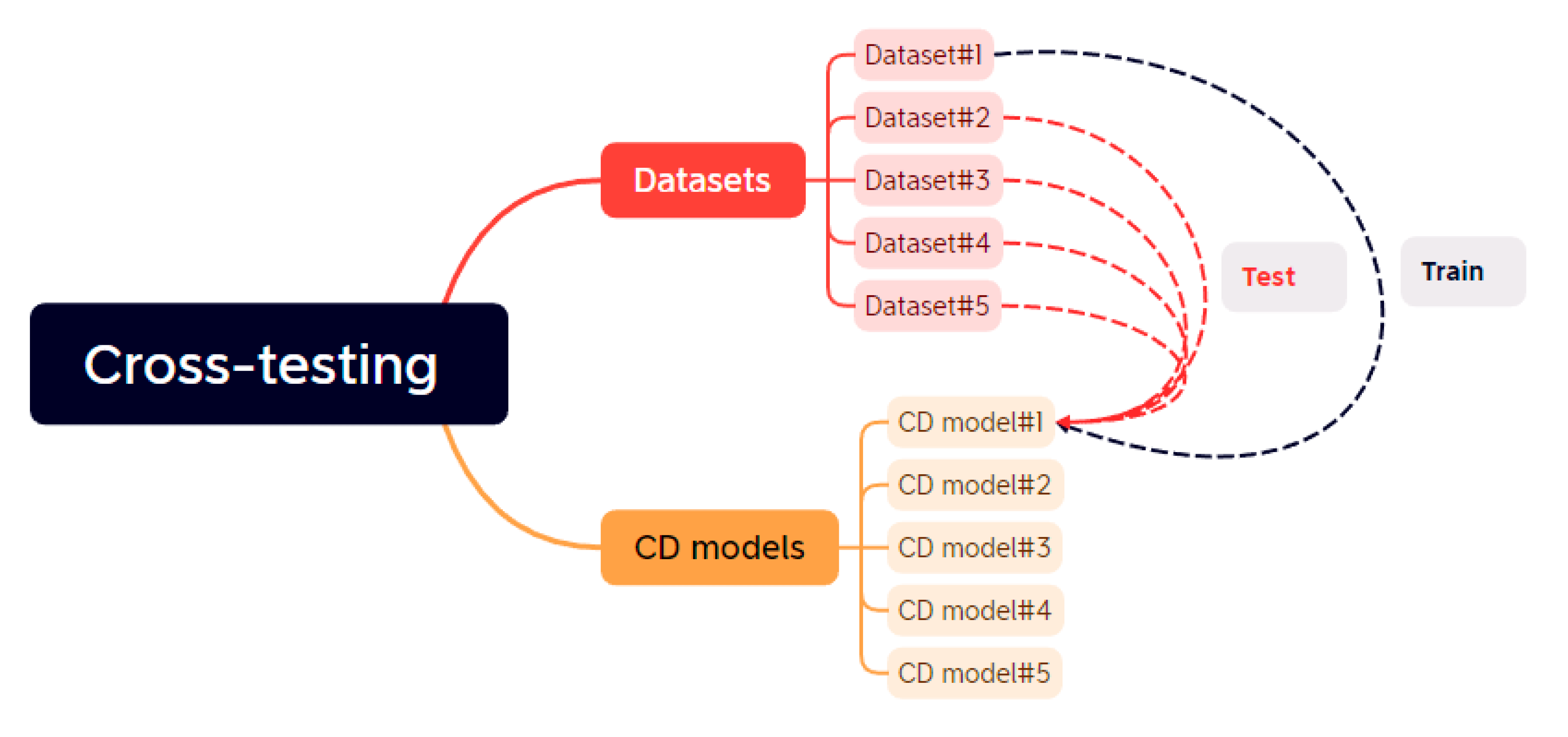
A significant challenge faced by deep learning change detection models pertains to their ability to generalize. This challenge arises from the necessity of CD models to accurately identify changes within diverse and complex datasets that deviate considerably from their training data. The primary goal of our cross-testing pipeline is to evaluate the generalization capacity of CD models across benchmark datasets and assess the impact of testing them on data distinct from their training set. This cross-testing seeks to determine whether CD models can effectively identify changes in various real-world scenarios and extend their learning to unseen contexts. Furthermore, it aims to uncover potential biases or limitations within the models’ training that might affect their real-world performance. The carefully chosen testing datasets exhibit variations in resolution, change classes, locations, and camera setups. They can be classified into building change datasets, and general change datasets, encompassing diverse change types.
Figure 2.
Illustration of the cross-testing.
3.3. A Multifaceted Approach to Contour-Based Analysis
The current approch include three related pipelines and are contour-level-based, the concept "contour" denotes interconnected curves or lines delineating the boundaries of changed objects that share the same intensity. conducting an experiment on the contour level, rather than at the image level, can offer valuable insights and provide fine-grained information. The three investigated phases are as follows:
- Performance sensitivity analysis based on the change size
A pivotal factor influencing the performance of our CD models is their sensitivity to changes of diverse sizes. To address this critical aspect, we have established a comprehensive pipeline that streamlines the comparative assessment of these models, specifically evaluating their capability to detect changes across various dimensions. For this evaluation, we necessitate a dataset that encompasses well-separable contours with different sizes in its ground truth images. Then we evaluate our CD models on each contour separately For each contour in the ground truth, we calculate the number of white pixels and evaluate it using our four CD models. Subsequently, we establish a relationship between each contour’s size in the ground truth and the performance metrics for the four models.
- Detection capability of challenging contours
Another critical aspect involves identifying scenarios in which the change detection (CD) models exhibit a complete inability to detect changes. Recognizing these challenging cases is instrumental in enhancing model performance. In this pipeline, we examine each contour within the ground truth dataset and assess its Intersection over Union (IoU) with the predictions from the four-CD models. If the IoU equals zero, it signifies that the contour is particularly challenging and remains undetected by the models. Subsequently, we proceed to compare the capabilities of these models in effectively detecting these challenging contours.
- Contour Count Comparison
Analyzing the disparity between the counts of predicted contours and ground truth contours is a fundamental aspect of the evaluation process in many applications such as building change detection. Because it offers valuable insights into the model’s treatment of contours, particularly in terms of whether it combines them or separates them. This aspect of model behavior is essential to understand, and contour count analysis can help reveal it. Here’s how it can provide this information:
Concatenation of Contours:
- When a model concatenates contours, it treats closely connected or neighboring building outlines as a single contour. This behavior can be indicative of the model’s tendency to merge adjacent changes that share similar properties or are part of the same structural unit.
- Contour count comparison may show that the model generates a smaller number of contours compared to ground truth when changes are closely related. This suggests that the model has a propensity to merge contours that are spatially connected.
Division of Contours:
- Conversely, when a model divides contours, it identifies subtle differences within closely situated building contours, which can lead to multiple smaller contours where the ground truth may have a single larger contour.
- In this case, contour count comparison may reveal that the model produces more contours than the ground truth for changes that are in close proximity or have intricate shapes. This indicates that the model dissects building outlines into multiple smaller components.
- Robustness Analysis with Respect to Different Image Corruptions
One of the foremost challenges confronting Change Detection (CD) models when applied to aerial images is the presence of noise. Aerial images are susceptible to various types of noise that alter their inherent intensity values. Noise is introduced into the images during acquisition or transmission, often due to factors like atmospheric interference or limitations in sensor quality. This noise can hamper the accurate recognition and analysis of the images.The impact of noise on the performance of Land Cover Change Detection (LCCD) models can be substantial. Therefore, the analysis and comparison of CD models based on their resilience to various forms of noise offer valuable insights into how noise levels affect the performance of these models. Additionally, such analysis can contribute to the development of strategies aimed at enhancing their robustness in the presence of noise
4. Materials and Methods
4.1. Data Collection: Datasets
In our work, we chose five benchmark land cover change detection datasets that are publicly available. Three of them are mainly building CD datasets LEVIR-CD, WHU-CD, and S2looking, and the other two datasets CDD and CLCD have multiple types of change so we can call them general CD datasets.
- LEVIR-CD [43]: is a valuable and large-scale dataset in the CD field. consists of 637 sets of Google Earth images with a resolution of 0.5 meters/pixel and a size of 1024 × 1024. Each set of images contains the image before and after the building changes and a corresponding label. The original images had been divided into 256 × 256 size images without overlap. The dataset was divided into a training set of 7120 images, 1024 for validation, and 2048 for testing.
- WHU-CD [44]: is a public building CD dataset consisting of a pair of aerial images of size 32507 × 15354 and has a high resolution of 0.075 meters/pixel. A default cropping of 256 × 256 was applied to it without overlap obtaining a training set of 6096 images, 762 in the validation set, and a test set of 762.
- S2Looking [45]:is a building change detection dataset that contains large-scale side-looking satellite images captured at varying off-nadir angles. It consists of 5,000 bi-temporal image pairs with a size of 1024*1024 and resolution ranging from (0.5 ~ 0.8 m/pixel) of rural locations over the world and more than 65,920 annotated change instances.
- CDD [46]: is a widely used dataset for change detection and it contains 11 pairs of remote sensing images obtained by Google Earth in different seasons with a spatial resolution ranging from 3 to 100 cm per pixel. After cropping the original image pairs into the same size of 256×256 pixels, thus generate 10000 image pairs for training, 3000 image pairs for validation, and 3000 image pairs for testing.
- Cropland Change Detection (CLCD) Dataset [47]: consists of 600 pairs of 512 × 512 bi-temporal images that were collected by Gaofen-2 in Guangdong Province, China with a spatial resolution of 0.5 to 2 m, each group of samples is composed of two images of 512 × 512 and a corresponding binary label of cropland change. A default cropping of 256 × 256 was applied to it without overlap.
4.2. State-of-the-Art (SOTA) CD Models
To validate the effectiveness of the proposed Framework in comparing and analyzing the CD models. we applied it to five of the SOTA land change detection models which achieved high-performance metrics with the Benchmark datasets such as LEVIR, WHU, and CDD datasets.
- BIT [48]: is a transformer-based feature fusion method, which combines CNN with transformer encoder-decoder structure. That allows for capturing effective and meaningful global contextual relationships over time and space.
- SNUNet [49]: This is a multilevel feature concatenation method that combines NestedUNet with a Siamese network. it also uses an Ensemble Channel Attention Module for deep supervision.
- Changeformer [50]: Transformer-based change detection method, which leverages the hierarchically structured transformer encoder and multilayer perception (MLP) decoder in a Siamese network architecture to efficiently render multiscale long-range details required for accurate CD.
- Tiny [51]: is a lightweight and effective CD model that uses a Siamese Unet to Exploit low-level features in a globally temporal and locally spatial way. It adopts a novel space-semantic attention mechanism called MIX and Attention Mask Block (MAMB).
- CSA-CDGAN [44]: is a CD network that uses a Generative Adversarial Network to detect changes and a channel self-attention module to improve the network’s performance.
The proposed Framework has five pipelines the first one performs cross-testing over five CD models, the next three pipelines perform contour-based analysis. and the last pipeline performs robustness analysis of the CD models by testing them in three noisy versions of the LEVIR dataset. the second and third pipelines applied only to the CD models trained on the LEVIR dataset. In the three pipelines, we evaluate the CD models based on precision, recall, F1 score, and PRD (explained in section 5.1)
4.3. Cross-Testing Pipeline
In that experiment we chose carefully five of the benchmark datasets, we can categorize them into two categories mainly building change datasets such as LEVIR, WHU, and S2looking whose mask contains changes on buildings, and general change datasets such as CDD and Cropland which contain different types of change such as buildings, roads, lakes, cars, and natural objects. We performed our experiment with five high-performing CD models SNUNet, Changeformer, Tiny, BIT, and CSA-CDGAN. The SNUNET model was trained on the CDD dataset, and the other four CD models were trained on the LEVIR dataset. We test each CD model with the five CD datasets.
4.4. A Multifaceted Approach to Contour-Based Analysis
In this approach, we conduct an extensive evaluation of our CD models using the LEVIR dataset which has a high-quality annotation. also, its ground truth images encompass a wide range of contours with diverse sizes and shapes. Each instance of the dataset contains the ground truth and the corresponding predictions of our four CD models because our analysis depends mainly on them. Within this approach, we have implemented three key pipelines, each serving a distinct purpose.
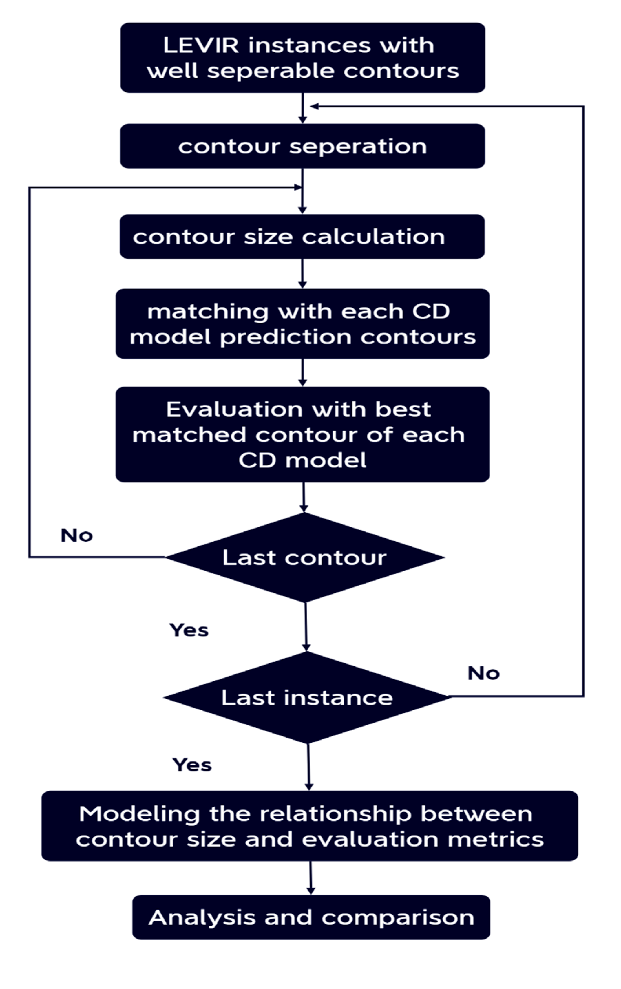
4.4.1. Performance Sensitivity Analysis Based on the Changed Contour Size
In our processing pipeline, we adopt a selective approach. First, we select instances within the dataset where the contours of the ground truth image and their counterparts in the predictions of our CD models exhibit significant separability. This selection ensures that we work with data points where the change detection is most discernible.
Subsequently, we employ a contour-matching algorithm to establish a one-to-one correspondence between the contours in the ground truth images and those in the model predictions for each of these chosen instances.
Following the contour matching process, we compute the change size for each contour and proceed to evaluate the performance of various change detection models. We measure key performance metrics such as precision, recall, F1 score, and PRD for each model, taking into account the matched contours.
To better understand the relationships between contour size and the performance metrics (precision, recall, F1, and PRD), we conduct detailed modeling. This modeling step allows us to uncover the intricate dependencies between these variables.
Lastly, we conduct a comprehensive analysis and comparative assessment of the change detection models, leveraging the insights gained from our modeling efforts. This analysis facilitates a deeper understanding of how the models perform under different circumstances, making it possible to identify trends and patterns that can inform model selection and optimization.
Figure 3.
The pipeline of the performance sensitivity analysis based on the change size.
4.4.2. Detection Capability of the Challenging Contours
Within this pipeline, our focus lies on evaluating the detection capabilities of our CD models, specifically regarding to challenging contours. These challenging contours are characterized as those within the ground truth data that at least one CD model fails to detect entirely. To identify these challenging contours, we calculate the Intersection over Union (IoU) between each ground truth contour and the corresponding prediction contours. If the IoU equals zero with any CD model’s prediction, we classify that contour as challenging. Subsequently, we conduct a comparative analysis of our CD models based on their effectiveness in detecting the maximum number of challenging contours. We applied that for each nonblack ground truth image in the LEVIR testing dataset
4.4.3. Contour Count Comparison
Within this pipeline, for each instance of the LEVIR dataset, we perform two key tasks: first, we count the number of contours in the ground truth, and second, we tally the number of contours in the prediction. Subsequently, we establish a mathematical relationship between these counts through regression analysis, producing a regression line. Finally, our analysis extends to the comparison of the resulting regression lines generated by our four CD models. We contrast them with the ’identity line,’ which forms a 45-degree angle, signifying a scenario where the number of contours in the ground truth perfectly matches the predicted contours.
4.5. Robustness Analysis with Respect to Different Image Corruptions
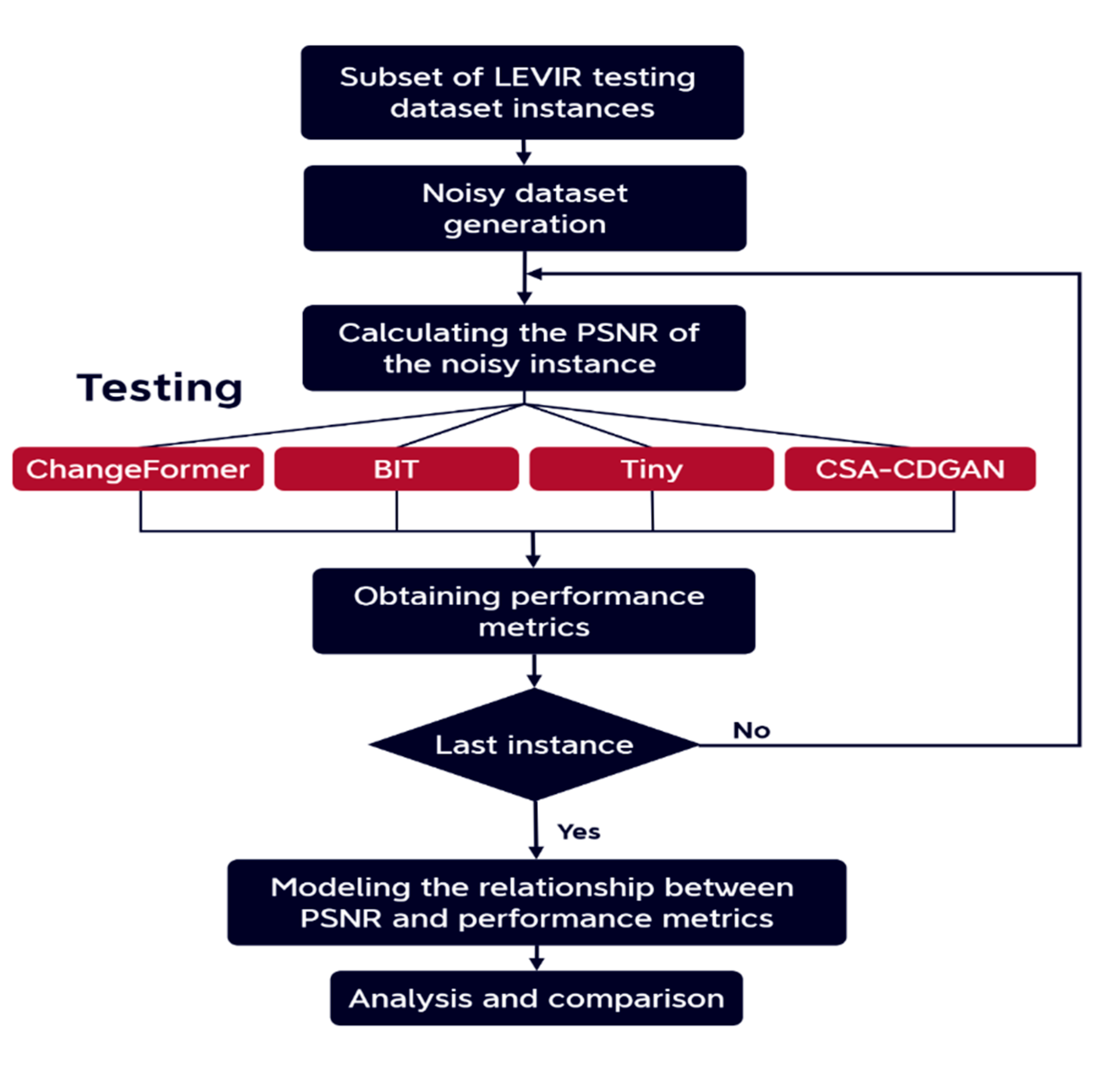
in the proposed pipeline, we analyze and compare the robustness of four state-of-the-art CD models to three common types of noise found in aerial images Gaussian noise, salt and pepper noise, and speckle noise. Figure 4 shows the overall experimental flow of the current study.
Figure 4.
Experimental flow.
At first, we will discuss the three common types of corruptions that can significantly affect the performance of the change detection models:
- Gaussian Noise: Gaussian Noise is a type of statistical noise characterized by a probability density function following the Gaussian distribution with a mean (μ) of 0 and a standard deviation (σ) that controls the amount of noise. It can arise due to various factors, including limitations in sensors, electrical interference, or atmospheric conditions.
- Salt and Pepper Noise: Salt and Pepper Noise, also known as Impulse Noise, arises from abrupt and sharp disruptions in the image signal. It appears in the image as random occurrences of white and black pixels. This type of noise is commonly attributed to malfunctioning image sensors.
- Speckle Noise: Speckle noise is known as multiplicative noise a prevalent artifact that can impair the interpretation of optical coherence in remote-sensing images. Its presence can substantially compromise the quality and precision of the images, rendering the identification and analysis of crucial features and structures challenging
- Peak Signal-to-Noise Ratio: It is a widely used metric for evaluating the quality of a corrupted or distorted image compared to the original image. the PSNR value is a metric that quantifies the ratio between the maximum potential power of a signal and the power of the noise or distortion that exists in the signal. If we have an input image I and its corresponding noisy image H, we can calculate the PSNR between the two images using the following formula:where MAX is the maximum possible pixel value in the image (e.g., 255 for an 8-bit grayscale image), and MSE is the mean squared error between the original image I and the noisy image H. The mean squared error is calculated as the average of the squared differences between the pixel values of the two images. higher PSNR values indicate lower levels of distortion or noise, while lower PSNR values indicate higher levels of distortion or noise.PSNR = 10 * log10((MAX^2) / MSE)
At first, we chose randomly 200 instances of the LEVIR testing dataset then we created three distinct noisy datasets from the original LEVIR dataset: Gaussian LEVIR, salt and pepper LEVIR, and speckle LEVIR. The generation process involved selecting each instance from the original LEVIR dataset and applying various levels of noise exclusively to image T1 using a Python environment. This process resulted in the creation of new instances, each comprising noisy T1, T2, and ground truth images.
To diversify the noisy datasets, we introduced different levels of noise to each instance. This intentional variation aimed to expand the dataset by incorporating instances with a range of noise levels. The applied noise levels were carefully chosen to ensure that the resulting noisy datasets exhibit a PSNR range with practical significance.
For each noisy dataset, we selected each instance and calculated the PSNR value between noisy and clear T1 images only because image T2 is clear. After that, we obtained the performance metrics of our four CD models BIT, Changeformer, CSA-CDGANs, and Tiny on that instance. The performance metrics are F1, Precision, Recall, and PRD. Then we modeled the relationship between the PSNR, and each performance metric based on the distributions of data between them. Finally, we analyzed and compared the CD models based on the modeling relationships we have.
5. Results and Discussion
5.1. Performance Metrics
Performance metrics are pivotal in the evaluation and comparative analysis of CD models, serving as the fundamental quantitative indices for assessing the effectiveness and reliability of each algorithm. These metrics are crucial for discerning the model’s ability to correctly identify and classify changes within the imagery data. Precision quantifies the model’s accuracy, representing the ratio of true positives (TP) to the sum of true positives and false positives (FP). It essentially measures the proportion of correctly identified changes out of all the detected changes. A high precision indicates a lower rate of false alarms, where the model has confidently and accurately discerned true changes from non-changes. Recall, also known as sensitivity, is the ratio of true positives to the sum of true positives and false negatives (FN). This metric assesses the model’s capability to detect all relevant instances of change. High recall denotes the model’s prowess in capturing the breadth of changes, minimizing the oversight of actual alterations within the observed landscape. F1 Score is the harmonic mean of precision and recall, providing a single metric that balances both the precision and recall of the model. It is particularly useful when seeking a composite measure of performance, as it conveys the trade-off between precision and recall. A superior F1 score is indicative of a model’s robustness in achieving both high accuracy and completeness in change detection.
Precision-Recall Distance (PRD) is a performance metric that computes the Euclidean distance between the model’s precision and recall values to the ideal point of perfect precision and recall (100,100). PRD encapsulates the overall deviation from the optimal performance, with a value of 0 representing ideal precision and recall, and 141.42 delineating the maximum possible distance, hence the worst performance. The PRD metric is integral to understanding the model’s overall reliability in a geometric context within the precision-recall space. In the technical lexicon of performance evaluation, these metrics collectively offer a comprehensive appraisal of a model’s efficacy. True positives (TP) are the instances where the model correctly identifies changes, true negatives (TN) where no change is correctly recognized, false positives (FP) where non-changes are incorrectly labeled as changes, and false negatives (FN) where actual changes are missed. These metrics are essential in ascertaining the strength and weaknesses of CD models, thus guiding advancements in the field and informing the selection process for practical deployment.
To compare the performance of the CD models we report F1, precision, Recall, and PRD scores regarding the change class as the primary quantitative indices. These metrics can be defined as follows:
where TP, TN, FP, and FN represent true positives, true negatives, false positives, and false negatives, respectively.
5.2. Cross-Testing Results
Figure 5 presented showcase the performance of various change detection (CD) models—SNUNet, Tiny, BIT, CDGAN, and Ch-Former (short for Changeformer)—across different datasets: LEVIR-CD, WHU, S2Looking, CDD, and Cropland. The performance is measured using four metrics: F1 score, Precision, Recall, and Precision-Recall Distance (PRD).
-
LEVIR-CD:
- Tiny model performs exceptionally well with the highest F1 score and Precision, indicating its effectiveness in identifying true changes with few false positives on this dataset.
- BIT and Ch-Former display competitive performance with relatively high Recall scores, suggesting they are good at identifying most actual changes, but possibly at the cost of more false positives, as indicated by lower Precision compared to Tiny.
- SNUNet and CDGAN lag behind the others, with CDGAN showing the lowest F1 score and Precision.
- PRD is lowest for Ch-Former, indicating a closer proximity to ideal Precision and Recall values.
-
WHU:
- Here, the models generally show lower performance compared to LEVIR-CD.
- Tiny again leads in F1 and Precision, but its Recall is surpassed by BIT, indicating BIT is better at capturing more true positives in this dataset.
- SNUNet struggles significantly across all metrics, highlighting its inability to generalize to this dataset effectively.
- CDGAN exhibits the lowest Precision, indicating a high rate of false positives.
-
S2Looking:
- This dataset poses a challenge to all models with drastically lower performance metrics across the board.
- Tiny manages the highest F1 score and Precision, albeit these scores are very low, showing that it still performs best among the models but is not particularly effective for this dataset.
- The Recall metric is extremely low for all models, especially for CDGAN, suggesting that all models fail to detect the majority of true changes in this challenging dataset.
- PRD values are significantly higher for all models, with Ch-Former having the highest, indicating a substantial deviation from ideal performance.
-
CDD:
- SNUNet excels remarkably in this context, showing near-perfect Precision and Recall, which implies it can detect almost all true changes with very few false positives.
- The other models exhibit drastically lower F1 scores and Precision, with Tiny and BIT also having low Recall.
- The PRD scores for these models are notably higher than SNUNet’s, highlighting their poorer performance on the CDD dataset.
-
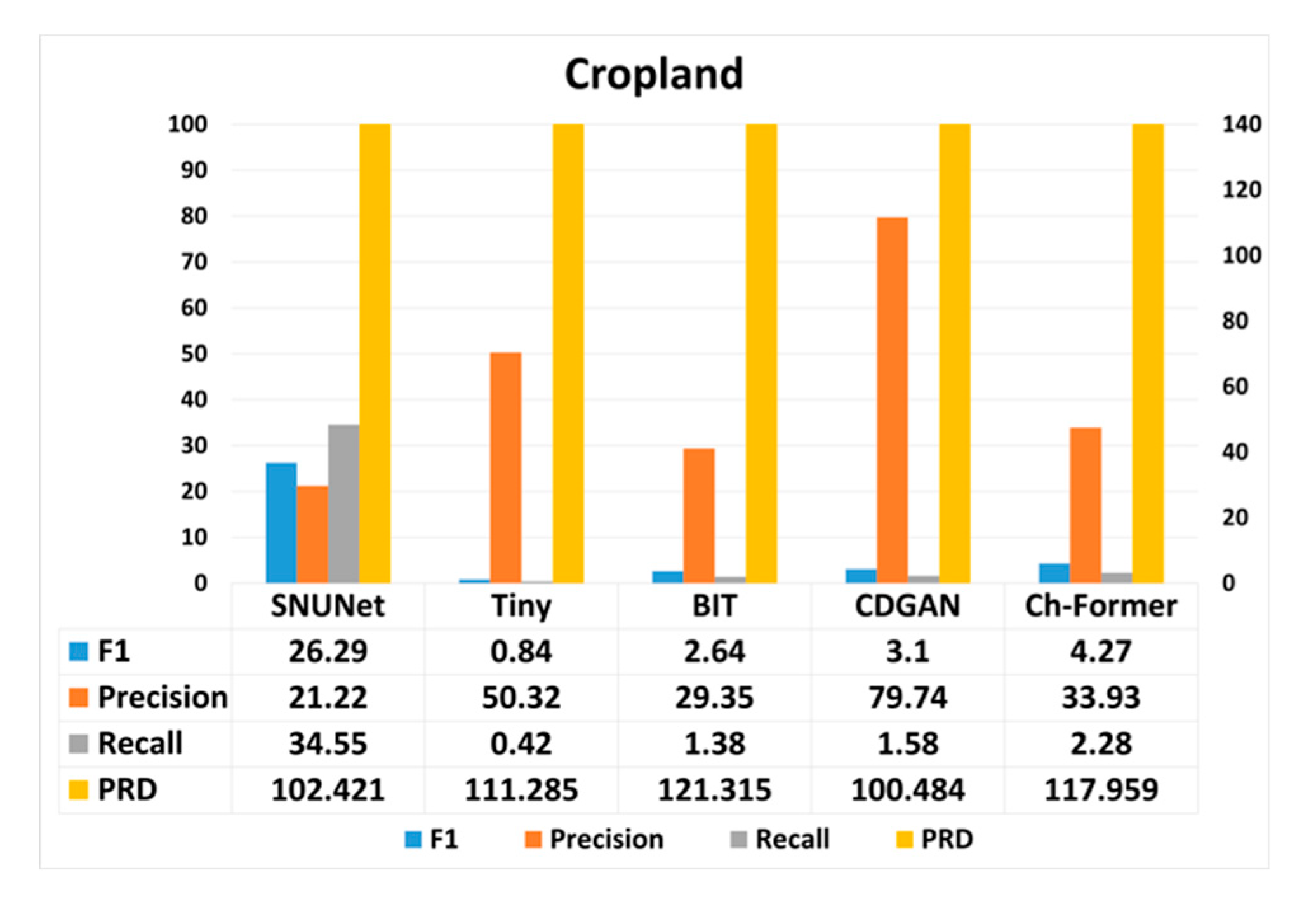
Cropland:
- All models demonstrate a decrease in performance compared to the CDD dataset, with no single model standing out significantly.
- SNUNet shows the highest F1 score and Recall but has lower Precision than CDGAN and Ch-Former.
- Tiny and BIT have very low F1 scores and Precision, indicating a struggle to correctly identify changes in this dataset.
- PRD values are high for all models, especially for Ch-Former, signaling a larger gap from optimal performance.
Figure 5.
The CD models performance on the benchmark datasets, note that Ch-Former is a brief of Changeformer and CDGAN is a brief of CSA-CDGAN.
Figure 5.
The CD models performance on the benchmark datasets, note that Ch-Former is a brief of Changeformer and CDGAN is a brief of CSA-CDGAN.
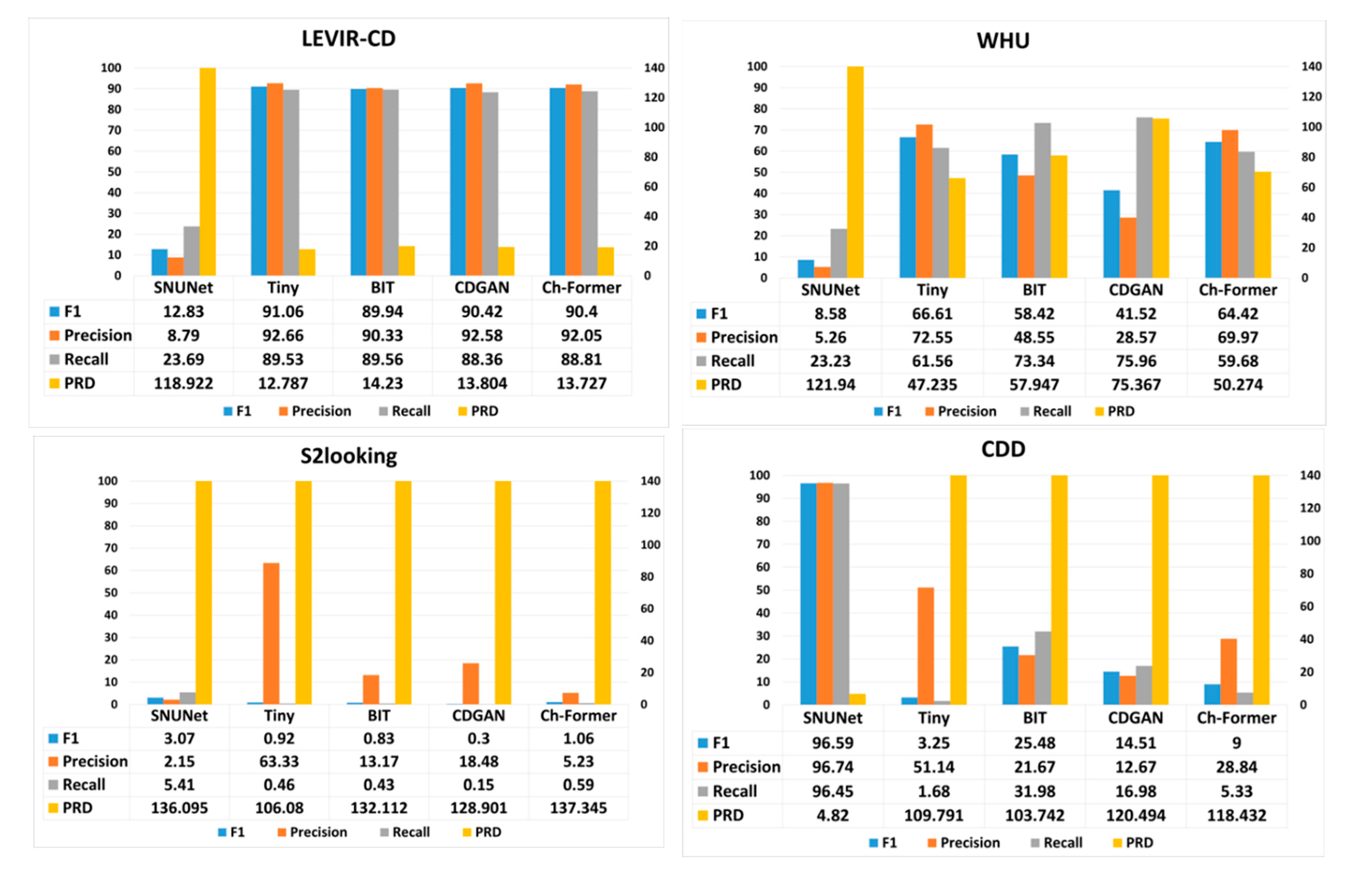
These results show that the CD models achieve the best performance metrics when the testing dataset has the same distribution as the training dataset. So, we find that BIT, Changeformer, Tiny, and CSA-CDGAN have the best performance metrics on the LEVIR dataset and SNUNet with the CDD dataset.
When testing CD models on the WHU dataset we find that SNUNet has a significant drop in the performance metrics, we also find that based on F1, precision, and PRD the tiny model achieves the best value then Changeformer, BIT, and CSA-CDGAN respectively. Also, CSA-CDGAN has the best Recall value then BIT and Changeformer have the lowest value.
When testing the CD models on the CDD dataset, the SNUNet achieved the best performance metrics. a significant drop in the performance of the models trained in the LEVIR dataset when testing them on the CDD dataset. Despite the difference between the two dataset distributions the BIT model had higher performance metrics compared with the other CD models trained on the LEVIR dataset which had a significant drop in their performance.
The performance metrics of the five CD models were totally dropped when tested on the S2looking dataset, which its images were taken with variating the off-nadir angles. This means that the setup of the camera by which the imagery dataset is collected plays a significant role in the CD model’s performance metrics and our five CD model’s architectures failed to generalize with that kind of dataset.
Finally, the results on the cropland dataset showed that the SNUNet had poor performance metrics although that model was trained on a similar dataset. The F1, Recall, and PRD values of the other CD models have been dropped totally. We also found that the CSA-CDGAN had the best precision value followed by Tiny, while the SNUNet had the smallest values.
5.2. Contour-Based Analysis Results
5.2.1. Performance Sensitivity Analysis Based on the Changed Contour Size
The majority of the contour sizes in the testing dataset ground truths are between [0 – 2100] pixels. Thus, we removed the outlier sizes outside of that range because that can help to focus our analysis on the relevant data and to increase the statistical power of our analysis. The descriptive summary of the testing dataset after removing the outliers as shown in Table 1.
The results provide insights into the characteristics of the dataset. Specifically, the wide variation in the values of the changed contour size. To show how the significant differences in the complexity and structure of the instances in the test dataset affect the performance metrics of our four CD models. More information is in Appendix A.
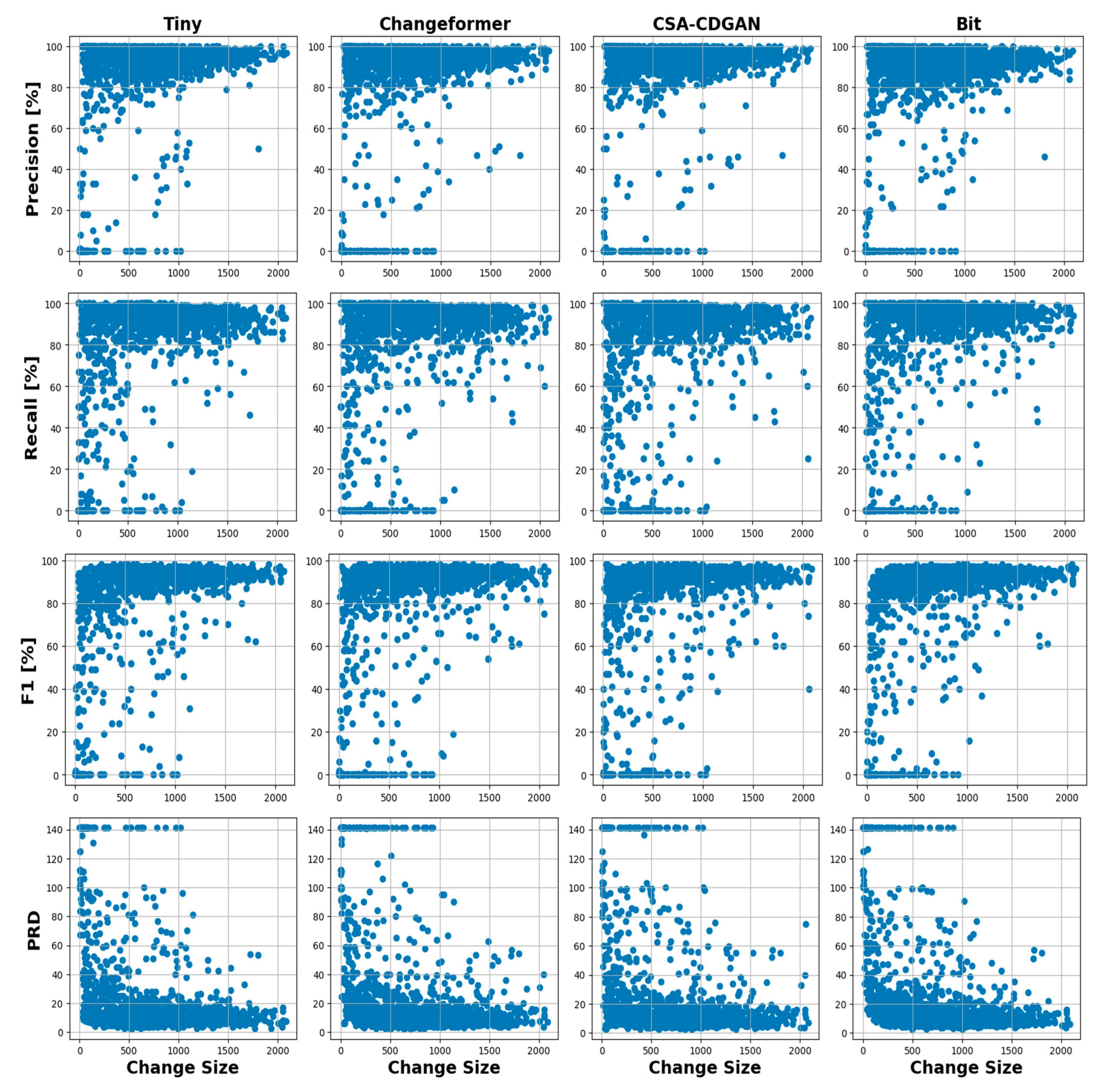
Figure 6 provides a visualization of the relationship between the changed contour size and the performance metrics of each CD model. The figure presents scatter plots for four change detection models—Tiny, Changeformer, CSA-CDGAN, and BIT—showing how each performs across different change sizes within a dataset in terms of Precision, Recall, F1 Score, and Precision-Recall Distance (PRD). The change size on the x-axis presumably represents the number of pixels that have changed between two time points within the images being analyzed.
Figure 6.
Scatter plots show the relationships between the average change size and performance metrics of the CD models.
Figure 6.
Scatter plots show the relationships between the average change size and performance metrics of the CD models.
The scatter plots showed the relationship between the change size and performance metrics of the CD model’s overall range of the average change sizes between [0 to 2100 pixels]. So, for further and deeper analysis and understanding of that relationship. We divided the change sizes into three ranges as shown in Table 2. The categorization of the change sizes has been done carefully based on the distribution of the data.
The Precision across all models, we observe that Precision tends to be higher when the change size is smaller, which might indicate that models perform better with less complex scenes or smaller change areas. Tiny and Changeformer maintain relatively high precision across most change sizes, while CSA-CDGAN and BIT experience more significant variability.
The Recall across all models show a trend where recall increases with the change size, suggesting they are better at detecting larger changes. Notably, Changeformer and BIT exhibit higher recall for smaller change sizes compared to the other two models, indicating their sensitivity to detect changes even when they cover a smaller area.
F1 Score across all models generally maintain a higher F1 Score as change size increases, indicating an overall better performance on larger change areas. Tiny seems to perform consistently well across a range of change sizes, which suggests a balanced approach between precision and recall.
PRD show the lower PRD values are better, and we can see that PRD generally decreases as the change size increases, indicating better performance on larger changes. Changeformer and BIT seem to have lower PRD scores for small change sizes, suggesting they are closer to the ideal precision and recall balance for smaller changes compared to the other models.
Overall, the performance metrics generally improve with the increase in change size for all models. Tiny appears to provide the best balance between detecting changes accurately (precision) and detecting most changes (recall), as evidenced by the high F1 Scores. Changeformer demonstrates a reliable detection capability across different change sizes, with particularly strong recall for smaller changes. CSA-CDGAN and BIT show more variability in performance, which may indicate a dependency on certain characteristics of the change or the image conditions that were not consistently present across all change sizes. There is a clear trend that all models perform better in detecting larger changes compared to smaller ones. Understanding these patterns is crucial for improving CD models, particularly for applications where detecting small changes is vital, such as early detection of environmental or urban changes.
After the division of the change sizes into three ranges, For each range we have fitted four linear regression models to model the relationship between the average change size and the four performance metrics as shown in Figure 7. This figure represent the performance of four different change detection (CD) models—BIT, CSA-CDGAN, Changeformer, and Tiny—as a function of the size of the change in the analyzed images. The graphs compare performance metrics: Precision, Recall, F1 Score, and Precision-Recall Distance (PRD) against ’change_size,’ which presumably measures the extent of change within the images, likely in pixel count.
Figure 7.
Concatenated linear regression models in the three change size ranges.
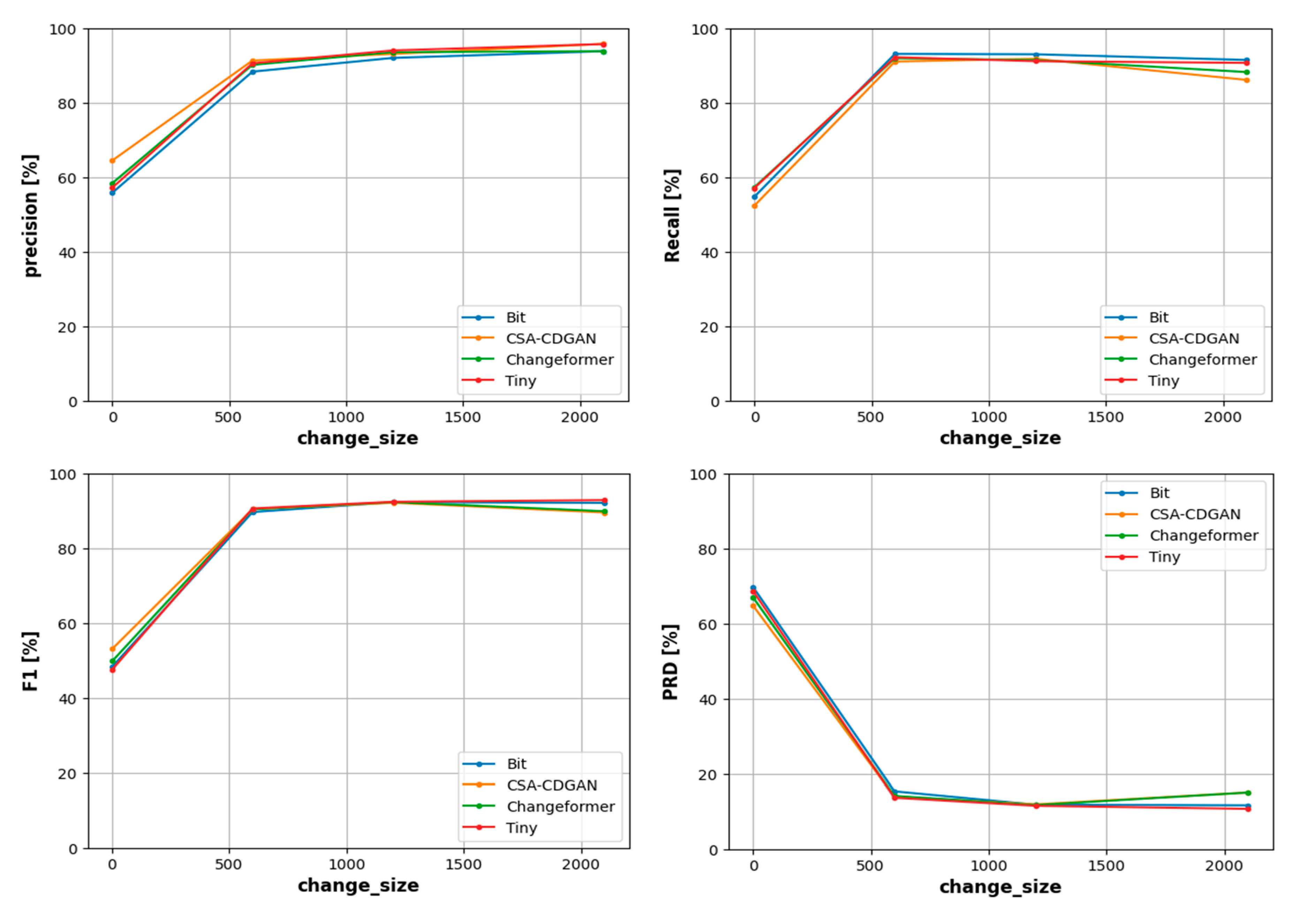
The precision show all models start with varied precision at the smallest change sizes but quickly converge as the change size increases. The precision for all models improves significantly as the change size increases up to around 500 pixels, beyond which the precision plateaus near perfect scores (100%). This indicates that all models are better at precisely identifying larger changes while having some difficulty with smaller change sizes.
The Recall show similar to precision, all models show an improvement in recall with increasing change size. The recall metric for all models levels off after a certain point, showing that once the change size is large enough, most actual changes are being correctly identified by the models. There’s less variation in recall among the models for larger changes, indicating that they are all reasonably good at detecting the majority of the true changes when those changes are large enough.
F1 Score show the F1 Score, being the harmonic mean of precision and recall, takes into account both the completeness and accuracy of the change detection. The graph illustrates that F1 Scores for all models are relatively lower for small changes but increase significantly as the size of the change increases, with all models reaching a plateau, indicating optimal performance. This suggests that the balance between precision and recall is better maintained by all models for larger change sizes.
PRD show the PRD graph shows a steep decline as the change size increases, indicating a significant improvement in model performance. After the initial drop, the PRD remains low and steady across all models, suggesting that the distance between the model’s precision-recall values and the ideal scenario (100%, 100%) is minimized. The low PRD values at higher change sizes suggest that the models are very effective at change detection when the changes are large.
The plateauing of the performance curves suggests a threshold effect, where performance increases with change size but only up to a certain point, beyond which additional increase in change size does not significantly improve model performance. The consistency in model performances for larger changes may indicate that these CD models are leveraging spatial context more effectively when the areas of change are substantial. The initial variability in the smaller change sizes can be attributed to the models’ sensitivity and specificity trade-offs, which are more critical when dealing with nuanced changes that may be prone to noise and other imaging artifacts. The PRD graph is particularly important as it inversely indicates model robustness—the lower the PRD, the closer the model is to an ideal performance state. The sharp initial decline suggests that the models rapidly approach an ideal state as the change size becomes sufficiently large. Overall, these graphs indicate that while all models are challenged by smaller change sizes, they perform similarly and well for larger change sizes. This has practical implications for selecting and using CD models in real-world applications where change sizes can be expected to vary greatly.
6. Analysis and Comparison
When examining the precision of change detection models relative to the size of the changes they are identifying, different models demonstrate varied strengths. For small-sized changes, the CSA-CDGAN model exhibits the highest precision, indicating its capability to accurately detect changes when they are minimal. Changeformer follows with the second-best performance in this category, while the Bit model ranks lowest, suggesting it may have difficulty in accurately identifying smaller changes.
As the size of the changes increases to medium and large, the Tiny model takes the lead, showcasing superior precision compared to its counterparts. This suggests that the Tiny model is particularly adept at maintaining accuracy as the complexity or extent of changes increases. CSA-CDGAN retains its strong position with the second-highest precision for larger changes, while Bit continues to struggle, indicating that it may be less suitable for tasks requiring high precision across a range of change sizes.
Delving deeper into the analysis, we can explore how these models perform in terms of recall, the ability to detect all actual changes. Regarding recall, the Tiny and Changeformer models excel at identifying the majority of actual changes in smaller-sized areas, while CSA-CDGAN falls short. This could imply that Tiny and Changeformer are more sensitive to subtle variations, which is crucial for applications where missing a change can have significant consequences. However, as the change size grows, the Bit model shows remarkable improvement, achieving the best recall for medium and large changes. This could indicate that while Bit may miss smaller changes, it becomes more reliable as changes become more pronounced.
To achieve a balanced perspective, we can consider the F1 Score, which incorporates both precision and recall. In the context of the F1 Score, CSA-CDGAN stands out for small-sized changes, with Changeformer trailing close behind. Tiny, however, scores the lowest, potentially due to a trade-off between its precision and recall. Yet, as we consider medium to large change sizes, Tiny takes the lead, indicating a better overall balance between precision and recall at these scales. It is noteworthy that the F1 Score for the Tiny model increases with the change size, in contrast to other models like CSA-CDGAN, which sees a decrease, particularly for large-sized changes.
The PRD metric further accentuates these observations. CSA-CDGAN achieves the closest to ideal performance for small changes, but as the change size grows, Tiny outperforms the rest, maintaining lower PRD values, thus staying closer to the ideal precision and recall values. Conversely, Bit shows the most significant deviation from ideal performance across all sizes, indicating areas for potential improvement.
The ability to detect challenging contours—areas within images where change detection models commonly fail—is crucial for model utility. Here, Tiny manages to detect a higher number of challenging contours compared to others, followed closely by Bit, Changeformer, and CSA-CDGAN. This highlights that while some models may excel in general performance metrics, their capability to handle intricate detection scenarios can vary substantially, underscoring the importance of specialized model tuning and algorithmic refinement to enhance performance in practical applications.
6.1. Detection Capability of Challenging Contours Results
The analysis includes a critical aspect of change detection models, which is their ability to discern challenging contours. Contours are essentially the boundaries of changed areas within an image, and the ability of a model to detect these accurately is a key measure of its effectiveness. The findings indicate that the ’Tiny’ model has the highest success rate, with 209 detected contours, hinting at its superior capacity for recognizing numerous changes in an image. ’Changeformer’ follows with 193 detections, ’Bit’ detects 171 contours, and ’CSA-CDGAN’ identifies 170, placing them in descending order of capability in this metric.
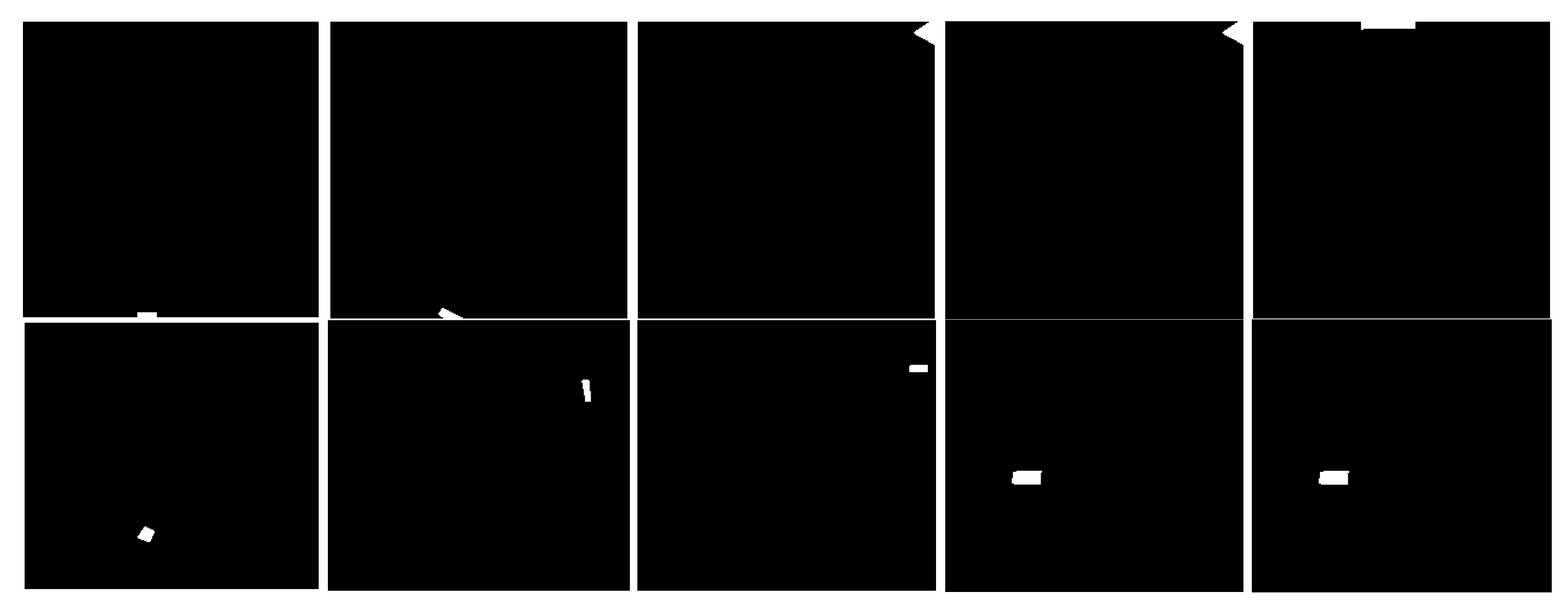
In Figure 8 shows a series of binary images used for evaluating the performance of CD models. The images appear to be binary masks, where white pixels represent areas of change, and black pixels represent unchanged areas. These images are used to determine if a change detection model can accurately identify changed areas (contours) within them. The scattered white pixels across the images, particularly those near the edges or isolated from larger areas of change, pose a significant challenge for CD models. Successfully detecting these small and fragmented contours is crucial, as it reflects the model’s sensitivity and precision. The performance of different models can be compared based on their ability to detect these subtle changes against the predominantly black background. This is an essential aspect of model evaluation, as the capacity to recognize minor alterations can be pivotal in applications such as environmental monitoring, urban development, and disaster assessment. Furthermore, Figure 8 exemplifies the inherent difficulty in detecting any pixel of a contour, emphasizing the importance of addressing this challenge in the development of CD models. The figure illustrates that most problematic contours are either small in size or located at the edge of the contours, which are regions where change detection models traditionally struggle. This highlights the need for advanced techniques in CD models to handle such intricate details effectively.
Figure 8.
Samples of the challenging contours in the LEVIR dataset.
6.2. Contour Count Comparison
Figure 9 illustrates the performance of various change detection models in terms of their ability to detect contours compared to the ground truth. The number of contours in the ground truth data is represented on the x-axis, while the number of contours predicted by the models is shown on the y-axis. The ’Identity Line’ serves as a reference that symbolizes a perfect alignment between the ground truth and the predictions. When a model’s prediction perfectly matches the ground truth, its line would align with the Identity Line. The accuracy of a model in predicting the correct number of contours increases as its line gets closer to the Identity Line. The line for Changeformer closely aligns with the Identity Line, indicating its high level of accuracy in predicting the number of contours. The deviation is minimal, suggesting that the changes are accurately estimated. Tiny’s performance exhibits a slight deviation from the Identity Line, suggesting that it tends to predict fewer contours than actually exist. This indicates a tendency to merge or overlook separate instances of change. Bit exhibits a more pronounced downward deviation, indicating a tendency to underestimate the number of contours more frequently than Tiny. This suggests that Bit may merge distinct contours into fewer, larger ones.
Figure 9.
Ground Truth vs. Prediction Contours.
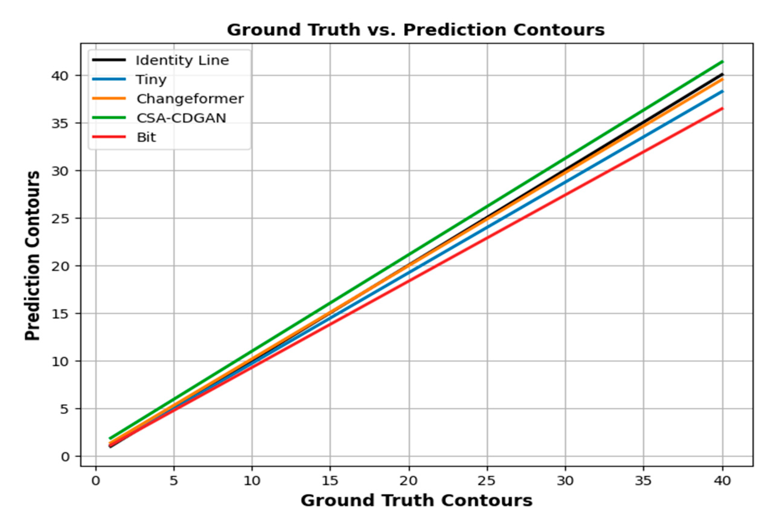
The line of CSA-CDGAN tends to deviate upward from the Identity Line, suggesting that it frequently predicts more contours than the ground truth. This indicates a tendency to divide what should be single contours into multiple detections. In evaluating the accuracy of CD models, the comparison of contour counts plays a vital role, especially in situations where the precise identification of individual contours is of utmost importance. The ability of each model to merge or divide contours can greatly impact its effectiveness for different change detection tasks. In nutshell, the Changeformer model seems to be the most accurate in predicting the number of contours present in the image compared to the actual number (ground truth).
6.3. Robustness Analysis with Respect to Different Image Corruptions Results
As shown in Table 3 each noisy dataset was constructed by considering the PSNR range. Also, to ensure the accuracy and comprehensiveness of our analysis, the number of instances in each noisy dataset varies, covering the respective PSNR range as extensively as possible.
6.3.1. LEVIR with Gaussian Noise Dataset
The robustness analysis with respect to different image corruptions, specifically Gaussian noise, is a test of how well change detection (CD) models can perform when faced with image quality degradation. Gaussian noise is a common problem in image processing that can significantly impact the performance of algorithms tasked with interpreting visual data.
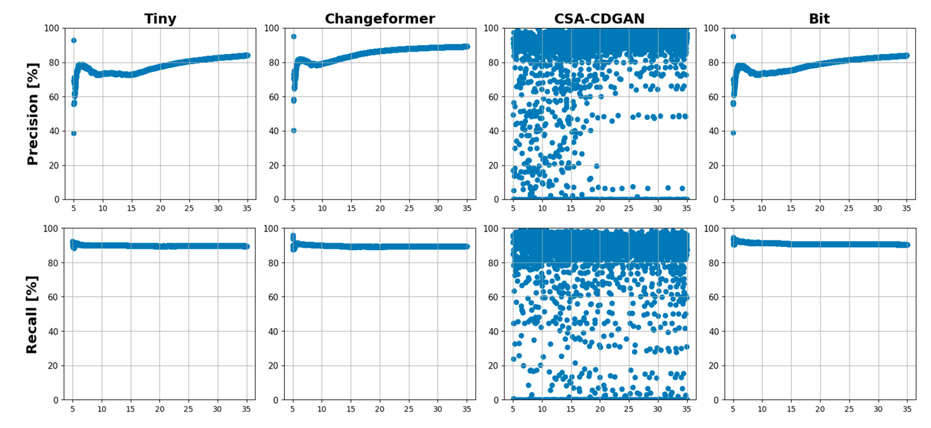
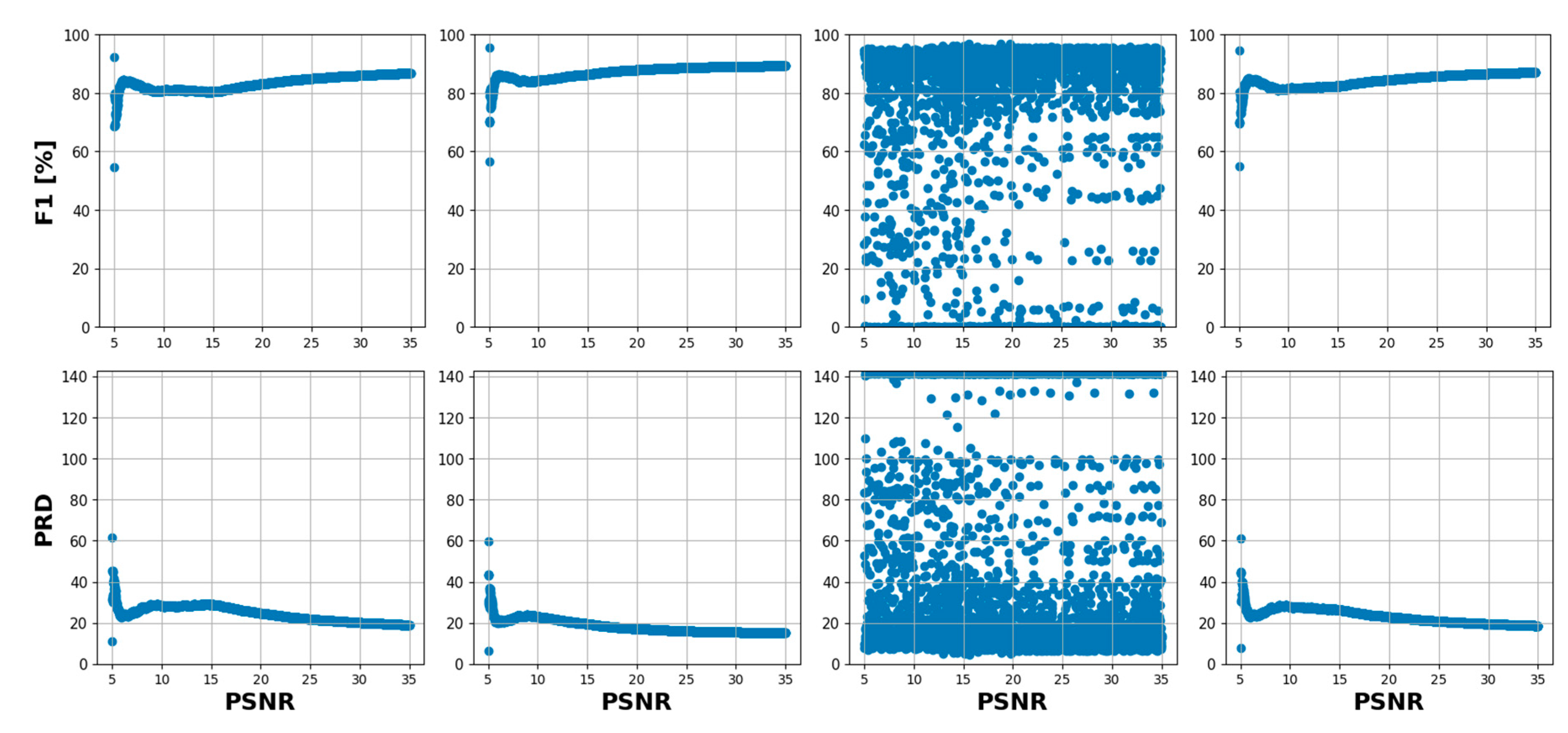
Figure 10 shows visual examples from the LEVIR dataset that have been artificially corrupted with Gaussian noise at varying levels of intensity, which are indicated by the Peak Signal-to-Noise Ratio (PSNR) range of [5 – 35]. PSNR is a measure of image quality with respect to the amount of noise present, with a higher PSNR indicating better image quality (less noise). Figure 11 depicts scatter plots and line charts, respectively, that illustrate the relationship between PSNR levels and the performance of four CD models (Tiny, Changeformer, CSA-CDGAN, and Bit) across several metrics: precision, recall, F1 score, and Precision-Recall Distance (PRD). In Figure 11, the scatter plots show a wide distribution of results, particularly for the CSA-CDGAN model, indicating variable performance across different levels of PSNR. This variability suggests that the model’s ability to accurately detect changes in the presence of noise is inconsistent.
Figure 10.
Samples from the Gaussian LEVIR dataset with added Gaussian noise.
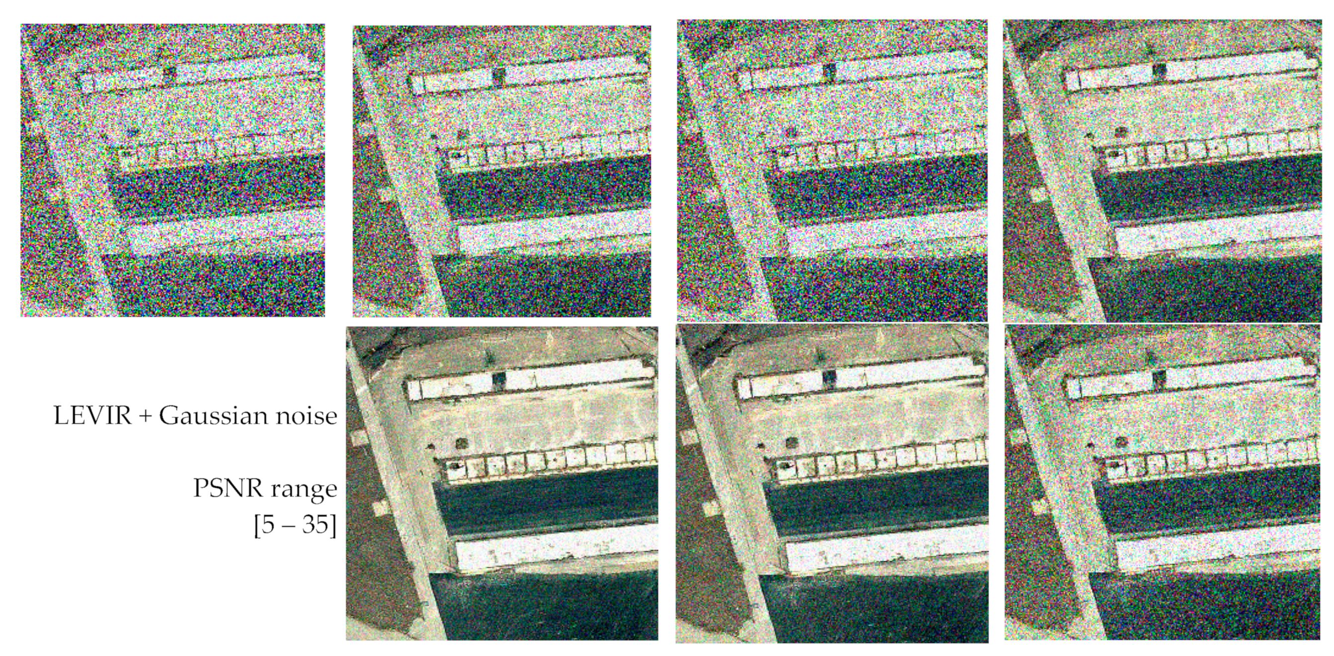
Figure 11.
Scatter plots show the relationship between PSNR and performance metrics of the CD models.
Figure 11.
Scatter plots show the relationship between PSNR and performance metrics of the CD models.
For further, deeper analysis and understanding of that relationship, based on the data distribution we divided the PSNRs into six ranges [5 – 6], [6 – 10], [10 – 15], [15 – 20], [20 – 25] and [25 – 30] dB. then for each PSNR range, we have fitted linear regression models to model that relationship as shown in Figure 12.
Figure 12.
illustrates the performance of CD models based on different evaluation metrics across various PSNR ranges.
Figure 12.
illustrates the performance of CD models based on different evaluation metrics across various PSNR ranges.
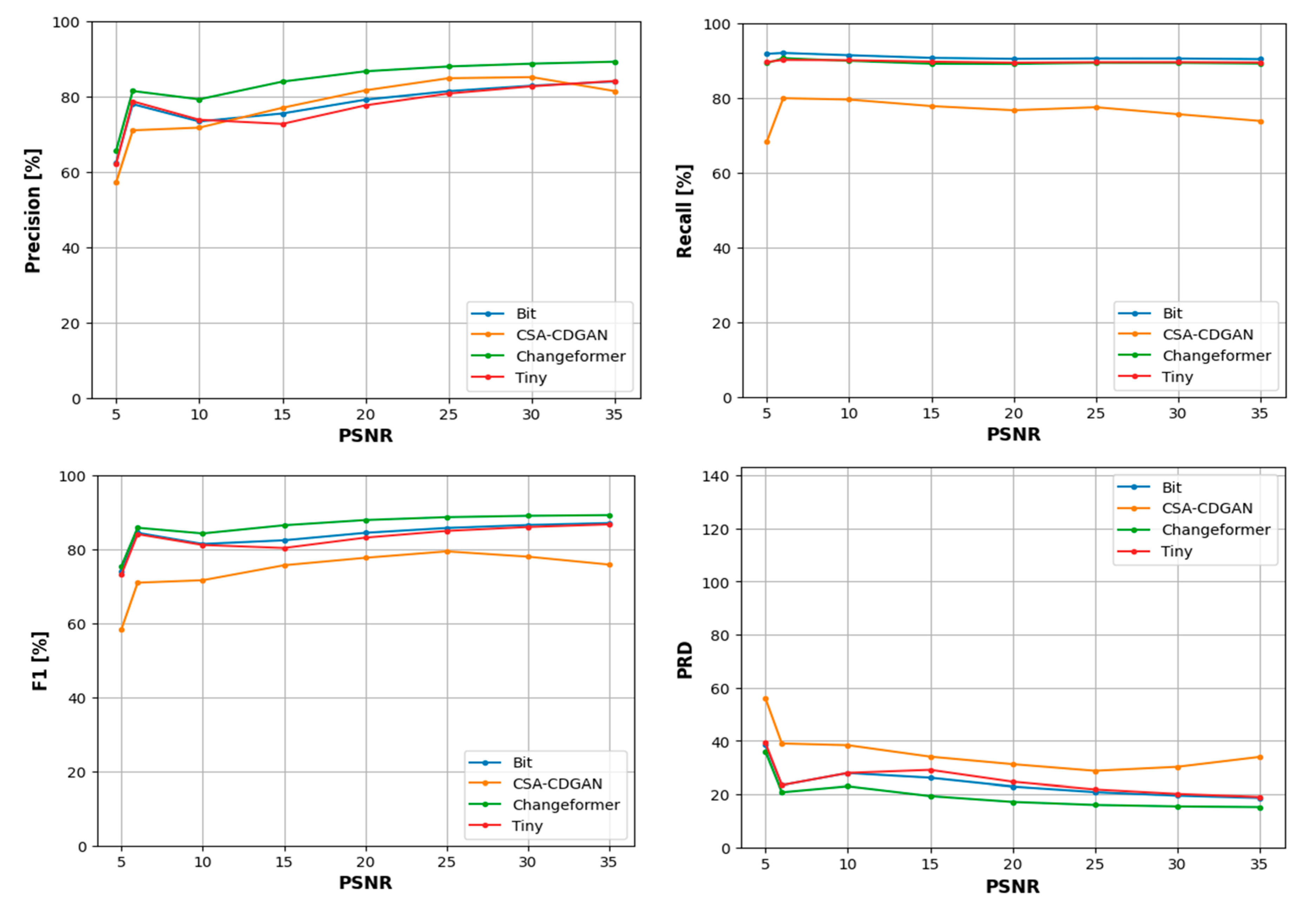
Figure 12 offers a more aggregated view of performance across different PSNR levels. The line charts allow us to compare the overall trend of each model’s performance as the noise level changes. Here are some detailed observations based on the tables and figures: Precision: Across the noise intensity range of [5 - 10] dB, Changeformer consistently outperforms the other models, followed closely by Bit and Tiny, which show similar results. CSA-CDGAN struggles the most in this aspect. Recall: Bit model consistently provides the best recall values, which means it is proficient at identifying all relevant instances of change in the noisy images. Changeformer and Tiny show competitive performance, while CSA-CDGAN again lags behind. F1 Score: The F1 score is a harmonic mean of precision and recall, offering a balance between the two. Changeformer leads in F1 score across the entire PSNR range, demonstrating an effective balance between precision and recall despite the noise. BIT also shows strong performance, while CSA-CDGAN has the lowest F1 scores. PRD: This metric represents the distance from the perfect score in the precision-recall space. A lower PRD indicates better performance. Changeformer has the lowest (and thus best) PRD scores, particularly in higher noise scenarios, followed by Bit. CSA-CDGAN consistently has the highest (worst) PRD values.
The drop in performance after adding Gaussian noise is quantified in the Table 5 and Table 6, with all models showing some degradation in their metrics, but to varying extents. The tables further emphasize that while all models are affected by noise, their ability to maintain performance varies, with Changeformer generally showing the least impact on precision and F1 score, and Bit maintaining recall robustly. Therefore, the analysis demonstrates that Changeformer has the best robustness against noise in terms of maintaining high F1 and low PRD scores, while Bit has the strongest recall. The variability in the models’ performance highlights the need for CD models that can withstand image quality issues commonly encountered in real-world scenarios.
6.3.2. LEVIR with Salt and Pepper Noise Dataset
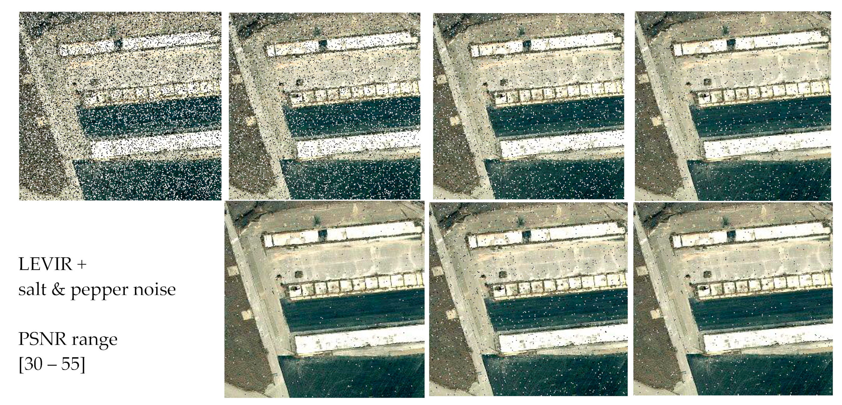
Figure 13 showcases samples from the LEVIR dataset that have been modified by introducing ’salt and pepper’ noise, which simulates a common type of digital image corruption where random pixels are set to black or white (hence the term ’salt and pepper’). This type of noise is particularly challenging for algorithms to handle as it can significantly disrupt image content, making it difficult to detect changes accurately. The PSNR range of [30 – 55] gives us an indication of the quality of these images, with higher values representing less noise and hence better quality.
Figure 13.
shows samples of the LEVIR testing dataset with salt and pepper noise.
In Table 7, the performance of four CD models on the salt and pepper noise-corrupted LEVIR dataset is summarized. This performance is measured using several key metrics:
- F1 Score: Indicates the balance between precision and recall. It is a useful measure when you want to seek a balance between detecting as many positives as possible (high recall) while ensuring that the detections are as accurate as possible (high precision).
- Precision: Shows the accuracy of the positive predictions. High precision means that an algorithm returned substantially more relevant results than irrelevant ones.
- Recall: Indicates the ability of the model to find all the relevant cases within a dataset. High recall means that the algorithm returned most of the relevant results.
- Precision-Recall Distance (PRD): Represents the Euclidean distance between the precision and recall values of a model to the ideal point of (100,100) on a precision-recall curve.

Table 7.
shows the CD model’s performance on salt & pepper LEVIR.
| CD model | F1 | Precision | Recall | PRD |
|---|---|---|---|---|
| Tiny | 78.08 | 82.2 | 74.75 | 31.04 |
| Changeformer | 84.76 | 80.29 | 90.02 | 22.27 |
| CSA-CDGAN | 75.73 | 79.37 | 77.03 | 33.57 |
| Bit | 82.91 | 76.01 | 91.45 | 25.55 |
Based on Table 7, the models’ performances are as follows: Changeformer stands out for its high F1 score and PRD, indicating a well-balanced performance between precision and recall, despite the noise. Bit model excels in recall, suggesting it is good at identifying relevant instances but may include more false positives, as evidenced by its lower precision. Tiny scores highest in precision but has the lowest recall, suggesting it is conservative in its predictions, ensuring what it detects is likely correct but at the risk of missing some changes. CSA-CDGAN has lower scores across all metrics, indicating it struggles more with this type of noise.
Table 8 highlights the drop in performance due to the added noise, showing that all models suffer a decrease in their metrics, but some cope better than others: Changeformer experiences a slight decrease in F1 score but manages to improve its recall, indicating that while precision drops, its ability to detect relevant changes is robust against salt and pepper noise. Bit maintains high recall despite a drop in precision, reinforcing its strength in identifying relevant instances even in noisy conditions. Tiny and CSA-CDGAN experience drops in both precision and recall, indicating a more significant impact from the noise. Overall, these tables indicate that while all models are affected by the introduction of salt and pepper noise, Changeformer and Bit exhibit stronger robustness, maintaining or even improving their recall. Tiny maintains the highest precision, potentially at the cost of missing some changes, and CSA-CDGAN is the most affected, struggling to balance precision and recall under noisy conditions. These findings underscore the importance of evaluating CD models across a range of noise conditions to ensure their utility in real-world applications where image quality may vary significantly.
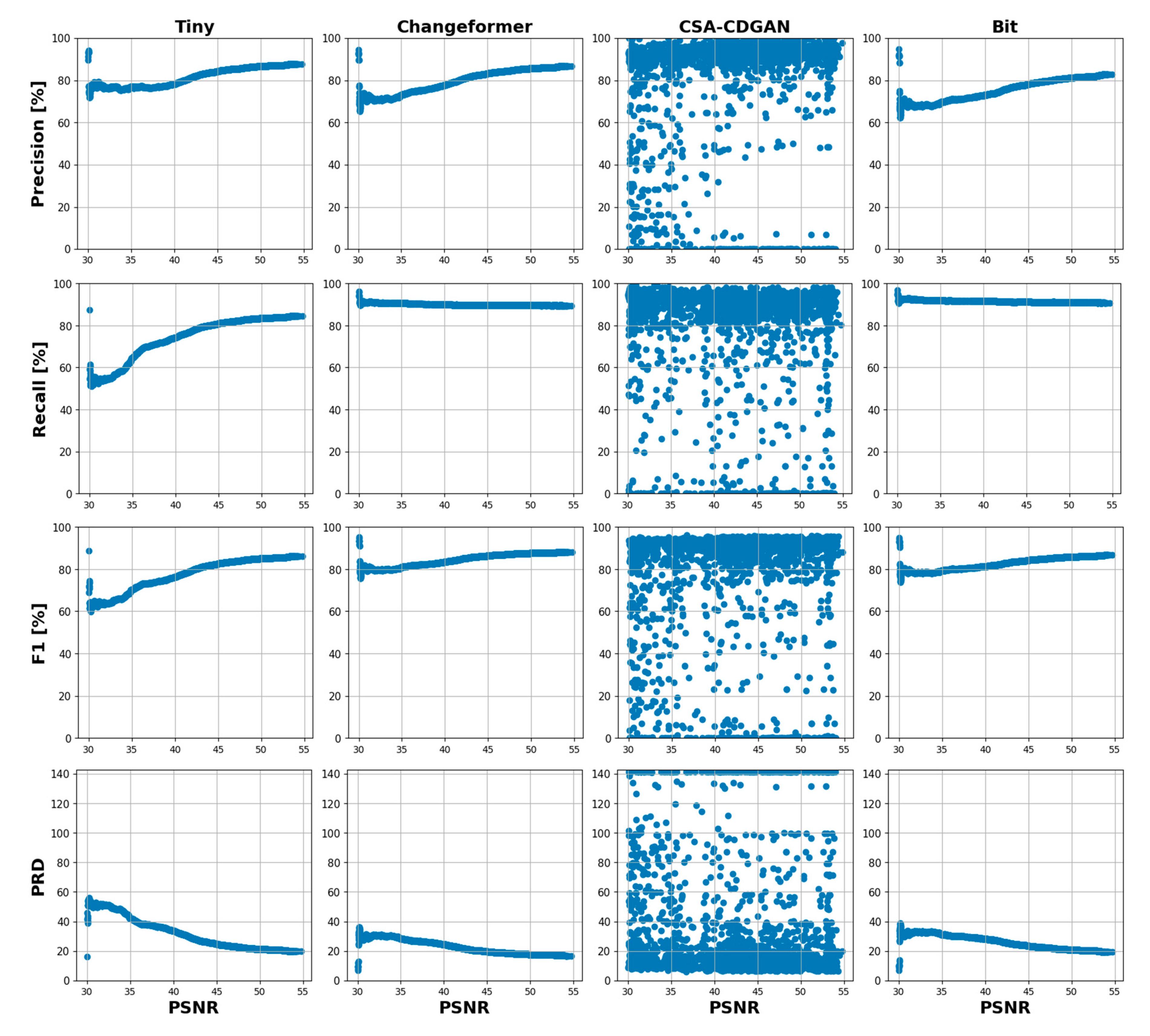
The scatter plots in Figure 14 demonstrate the relationship between the PSNR and the performance of four CD models across various noise conditions. PSNR is commonly used as a measure of image quality degradation due to compression or noise, with higher values indicating better image quality (less noise). To understand the relationship, based on the data distribution we divided the PSNRs into five ranges [30 – 35], [35 – 40], [40 – 45], [45 – 50], and [50 – 55] dB. Then for each PSNR range, we have fitted linear regression models to model the relationship between the PSNR and the four-performance metrics as shown in Figure 15. Each row in Figure 14 corresponds to a different performance metric (Precision, Recall, F1, PRD) for the CD models Tiny, Changeformer, CSA-CDGAN, and Bit, with each dot representing a different image in the noisy dataset. The horizontal axis shows the PSNR values, while the vertical axis shows the performance metric percentages. A high concentration of points near the top of the graph would indicate better performance. Precision: Across most models, as the PSNR increases (less noise), the precision either remains relatively stable or improves slightly, indicating that noise has a variable impact on the accuracy of positive predictions. Recall: Similarly, recall tends to increase with higher PSNR for most models, suggesting that as image quality improves, the models are better able to detect all relevant instances of change. F1 Score: This score remains relatively stable across PSNR values for most models, implying a balanced performance despite varying noise levels. PRD: Lower PRD values near higher PSNR values suggest that the models’ predictions are closer to the ideal precision and recall values when the image quality is better.
Figure 14.
Scatter plots show the relationship between PSNR and performance metrics of the CD models.
Figure 14.
Scatter plots show the relationship between PSNR and performance metrics of the CD models.
In the analysis of CD model performance across varying PSNR ranges, the F1 score, which combines precision and recall, shows that Changeformer consistently outperforms the other models between 30 to 40 dB, and continues to lead up to 55 dB. The Bit model ranks second in performance, indicating its robustness. However, Tiny struggles as noise increases, reflected by its lower F1 scores.
When focusing on precision alone, Tiny excels in the higher PSNR range of 30 to 35 dB, suggesting it can accurately predict changes when noise levels are lower. However, its precision advantage diminishes as noise increases. In contrast, CSA-CDGAN shows the least consistent precision, especially at lower PSNR levels (higher noise). Interestingly, the performance dynamics shift in the 40 to 45 dB range, where CSA-CDGAN steps up as the leading model, followed by Tiny. But as noise continues to increase beyond 45 dB, Tiny regains its top position with the least precision drop, maintaining it through to the 50 to 55 dB range.
For recall, the Bit model demonstrates superior performance in correctly identifying relevant instances of change from 30 to 45 dB, maintaining this lead as the PSNR range extends to 55 dB. Changeformer follows Bit closely, while CSA-CDGAN presents the lowest recall, indicating challenges in detecting true positives amidst higher noise levels.
Lastly, the PRD metric, which measures the combined deviation of precision and recall from their ideal values, shows Changeformer achieving the closest proximity to ideal performance, followed by Bit in the 30 to 40 dB range. As noise becomes more prominent, Changeformer continues to maintain the lead in PRD, suggesting its predictions remain relatively unaffected by the increase in noise levels.
These observations underscore the importance of choosing the right CD model based on the noise characteristics of the dataset. Changeformer appears to be a robust choice across most noise conditions, while Bit is noteworthy for its recall. Tiny, although excelling in precision at lower noise levels, requires careful consideration due to its performance variability with increasing noise.
Figure 15 visualizes the performance of the CD models across different PSNR ranges, as determined by linear regression modeling. These lines represent the trends in the data, providing a clearer view of how each model’s performance metrics change with the PSNR.
- For F1 and PRD scores: Changeformer consistently outperforms the other models, suggesting that it maintains a good balance between precision and recall and is close to the ideal values even as noise increases.
- In terms of precision: Tiny excels in the lower noise levels (higher PSNR values), but its performance varies more than CSA-CDGAN at higher noise levels. CSA-CDGAN tends to maintain more consistent precision across a wider range of PSNR values.
- Regarding recall: Bit outperforms the other models significantly across most of the PSNR range, indicating its robustness in detecting relevant changes even in noisier images.
The overall analysis indicates that Changeformer is generally the best-performing model with respect to balancing precision and recall across different noise levels, followed closely by Bit. Tiny, while excelling at precision in less noisy images, tends to struggle more as noise increases. CSA-CDGAN shows a more uniform performance across the noise spectrum but generally underperforms compared to Changeformer and Bit. These insights are crucial for developing robust CD models that are resilient to image quality variations, which is often the case in real-world scenarios.
4.4.3. LEVIR with Speckle Noise Dataset
Figure 16 presents samples from the LEVIR dataset with speckle noise introduced, spanning a PSNR range of 29.35 to 39 dB. This type of noise is characterized by the granular interference visible in the imagery, resembling a speckled pattern, which can challenge change detection (CD) algorithms. The performance metrics of the CD models on the speckle noise-affected LEVIR dataset are as follows: Tiny displayed an F1 score of 74.46, a precision of 63.85%, and a remarkable recall of 89.5%, indicating a strong ability to identify relevant changes despite the presence of noise. However, its precision suffered significantly, leading to a PRD of 37.66. Changeformer showcased an F1 score of 75.54, with better precision at 66.14% compared to Tiny, and a slightly lower recall of 88.26%. Its PRD of 35.86 suggests it maintained a balanced performance between precision and recall amidst noise. CSA-CDGAN scored an F1 of 72.12, precision at 70.3%, and a recall of 82.83%, achieving the highest precision yet the lowest recall among the models. Its PRD stands at 37.32, reflecting a moderate distance from ideal performance metrics. Bit produced an F1 score of 74.6, precision of 63.52%, and the highest recall among the models at 90.56%, indicating its strength in detecting true positives. Its PRD is 37.69, similar to Tiny’s, implying a comparable balance between precision and recall. Post noise introduction, the metrics reveal some interesting shifts: Tiny’s metrics dropped by 10.71 points in F1, 25.21 points in precision, while its recall increased by 6.71 points, and its PRD rose by 16.99 points. Changeformer’s performance decreased by 9.82 in F1 and 24.04 in precision, but its recall and PRD improved slightly by 5.72 and 15.58 points, respectively. CSA-CDGAN experienced a 6.33 decrease in F1 and a 13.7-point drop in precision, though its recall went up by 6.54 points, and PRD increased by 7.02 points. Bit showed a decline of 10.54 in F1 and a notable 23.65-point decrease in precision, yet its recall increased by 6.5 points, and its PRD went up by 16.91 points.
The increased recall values across the models after the introduction of speckle noise suggest an interesting tendency of the CD models to maintain, or even improve, their sensitivity to actual changes in noisier environments. However, the significant precision loss indicates a trade-off, as the models also incorrectly identify more non-changes as changes, which could be due to the speckle noise interfering with the models’ ability to distinguish between actual changes and noise artifacts. The careful balance between detecting changes (recall) and avoiding false alarms (precision) is crucial in noisy conditions, and these results highlight the resilience of these models to some extent, with BIT and Changeformer showing noteworthy robustness in recall, while CSA-CDGAN maintains the highest precision despite the noise challenge.
Table 10.
Drop in performance after adding speckle noise.
| CD model | F1 | Precision | Recall | PRD |
|---|---|---|---|---|
| Tiny | -10.71 | -25.21 | 6.71 | 16.99 |
| Changeformer | -9.82 | -24.04 | 5.72 | 15.58 |
| CSA-CDGAN | -6.33 | -13.7 | 6.54 | 7.02 |
| BIT | -10.54 | -23.65 | 6.5 | 16.91 |
Figure 17 and Figure 18 depict scatter plots and line charts illustrating the performance of various CD models across different PSNR ranges, which quantify the level of noise in images from the LEVIR dataset. understanding of that relationship, based on the data distribution we divided the PSNRs into four ranges [29.35 - 29.5], [29.5 - 30], [30 - 31], and [31 - 39] dB. then for each PSNR range, we have fitted four linear regression models to model the relationship between the PSNR and the four- performance metrics as shown in Figure 18. Here’s a breakdown of their performance metrics, analyzed across the specified PSNR ranges:
F1 Score:
- At PSNRs between 29.35 and 29.5 dB, amidst the highest noise intensity, CSA-CDGAN leads with superior F1 scores, suggesting robustness against noise, while Tiny is close behind. BIT lags with the lowest scores.
- Within the PSNR range of 29.5 to 30 dB, Tiny excels, indicating its effectiveness in moderately noisy environments. BIT and Changeformer offer competitive performance, and CSA-CDGAN falls behind.
- For PSNRs from 30 to 31 dB, Changeformer rises to the top, surpassing all models, which indicates its efficient handling of this specific noise level. BIT and Tiny remain close contenders.
- When PSNRs span 31 to 39 dB, CSA-CDGAN consistently achieves the highest F1 scores, denoting its capacity to maintain change detection accuracy over a wide noise range. Changeformer also shows robust performance, while Tiny trails with lower F1 scores.
Precision:
- In the highest noise bracket (29.35 - 29.5 dB), CSA-CDGAN’s precision is unrivaled, suggesting it’s less prone to false positives under severe noise conditions. Changeformer follows, and BIT exhibits the least precision.
- At PSNRs of 29.5 to 30 dB, Changeformer leads in precision, implying its discernment between noise and actual changes is optimal. Tiny is slightly behind, and CSA-CDGAN has the lowest precision, indicating more false positives.
- From PSNRs of 30 to 39 dB, CSA-CDGAN remains the precision leader, demonstrating its consistent ability to accurately detect changes across varying levels of noise, followed by Changeformer. Tiny and BIT show less precision, suggesting a higher rate of false positives.
Recall:
- In the range of 29.35 to 29.5 dB, Tiny and Changeformer exhibit the best recall, indicating their strength in identifying all relevant changes. BIT shows the lowest recall, potentially missing some true changes.
- For PSNRs between 29.5 and 30 dB, Tiny tops the recall metric, Changeformer and BIT are close, and CSA-CDGAN has the lowest recall, indicating missed detections of actual changes.
- Between 30 and 31 dB, Changeformer outperforms in recall, suggesting it misses fewer actual changes at this noise level. BIT and Tiny are comparable, while CSA-CDGAN has the lowest recall.
- From 31 to 39 dB, CSA-CDGAN surpasses others in recall, showing its consistent detection of changes across this noise spectrum. Changeformer follows, with Tiny showing the lowest recall, suggesting possible overlooked changes.
PRD (Precision-Recall Distance):
- At PSNRs of 29.35 to 29.5 dB, CSA-CDGAN showcases the best PRD, indicating a closer approximation to the ideal (100,100) point. Changeformer and Tiny have similar PRDs, while BIT has the highest PRD, suggesting a greater deviation from the ideal values.
- Between 29.5 and 30 dB, Changeformer and Tiny show advantageous PRDs, while CSA-CDGAN ranks lowest, indicating a larger deviation from ideal performance.
- In the PSNR span of 30 to 31 dB, Changeformer demonstrates an excellent PRD, implying a strong balance between precision and recall. BIT and CSA-CDGAN have similar PRDs, and Tiny has the highest PRD.
- For PSNRs from 31 to 39 dB, CSA-CDGAN achieves the best PRD, with Changeformer trailing closely. Tiny has the highest PRD, suggesting its performance is furthest from the ideal.
Figure 17.
Scatter plots show the relationship between PSNR and performance metrics of the CD models.
Figure 17.
Scatter plots show the relationship between PSNR and performance metrics of the CD models.
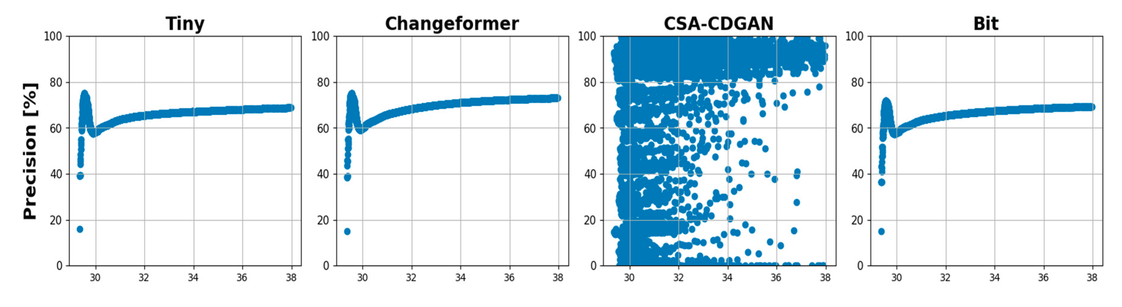
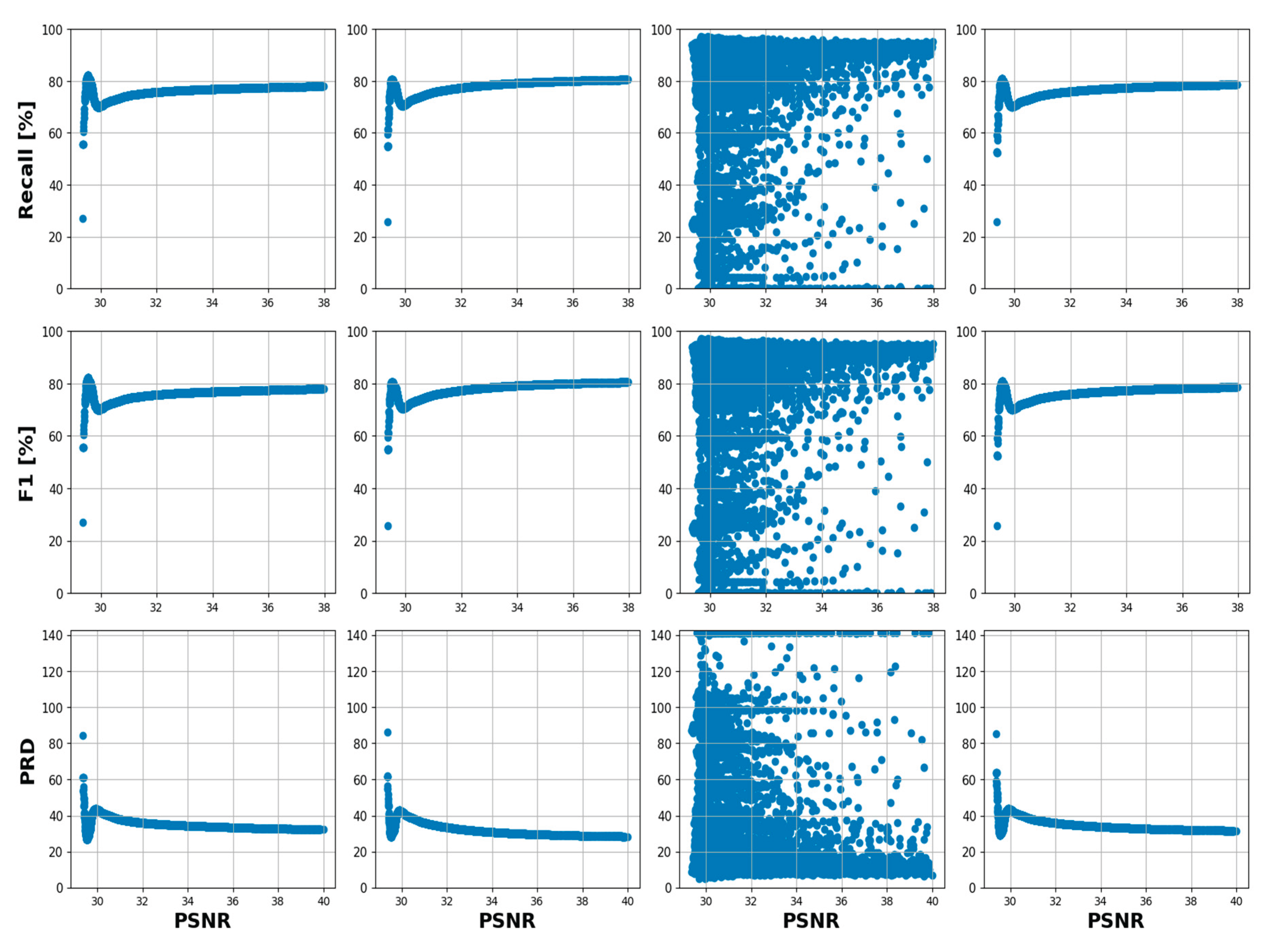
Figure 18.
illustrates the performance of CD models based on different evaluation metrics across various PSNR ranges.
Figure 18.
illustrates the performance of CD models based on different evaluation metrics across various PSNR ranges.
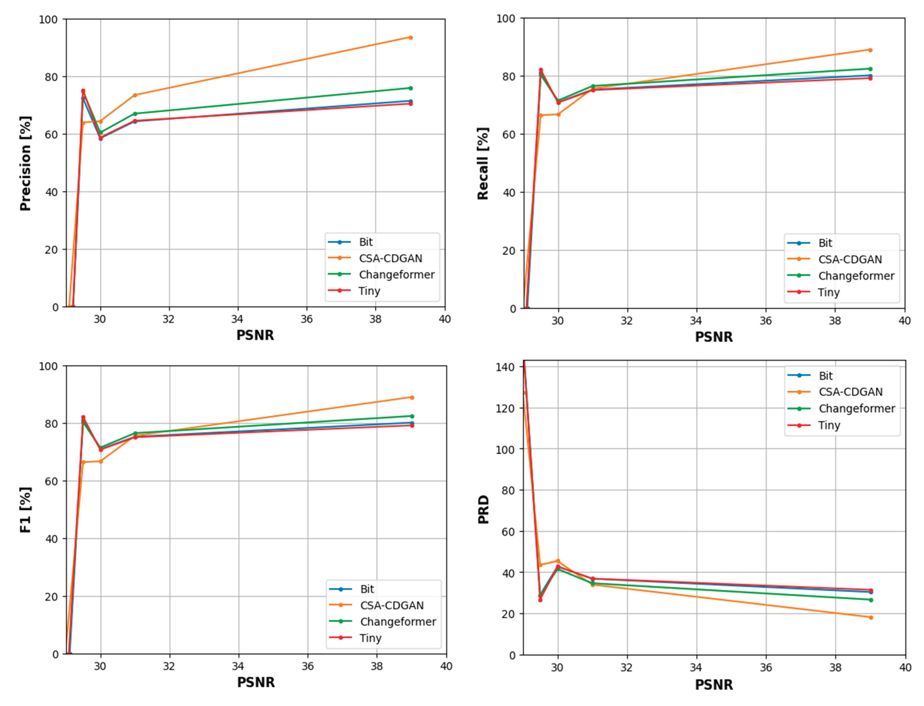
These analyses indicate that while noise levels universally impact the performance of CD models, their effects are nuanced, with each model showing strengths and weaknesses across different PSNR ranges. The metrics suggest that CSA-CDGAN and Changeformer are more robust to noise, particularly in maintaining precision and recall balance, while Tiny and BIT experience more significant performance fluctuations. This insight into model behavior in noisy conditions is critical for choosing and fine-tuning CD models for practical applications where image quality can vary widely.
7. Conclusion
This research explores the complex relationship between the effectiveness of CD models, the accuracy of aerial and satellite imagery, and the ability to withstand different sources of noise. Deep learning in the field of land cover change detection has produced a variety of models, each claiming to have excellent performance metrics. Nevertheless, the increasing number of models poses a challenge when it comes to selecting the right one, especially due to the lack of widely available benchmarks for thorough performance analysis and comparison. We presented and explained a flexible, scalable framework designed for the systematic assessment and comparison of CD models. This innovative framework is constructed using three interconnected pipelines—testing across different datasets, evaluating under challenging conditions, and conducting a detailed analysis of performance sensitivity based on the magnitude of changes. The utilization of this framework on five modern CD models—Changeformer, BIT, Tiny, SNUNet, and CSA-CDGAN—highlighted its effectiveness in identifying the strengths and weaknesses of these models. The findings from this exercise are crucial for evaluating and comparing these models, providing valuable information about their individual strengths and weaknesses. The framework proposed is a significant advancement in CD research, offering the potential to greatly increase the practicality of CD models. This work sets the stage for future research to build upon, offering a thorough comparison of existing CD models and establishing a standard for developing strong frameworks. Future avenues of research invite further investigation into the integration of these findings with wider computer vision tasks and the development of innovative models that embody the combined strengths identified and it has the potential to greatly advance the field of change detection technologies.
Author Contributions
A.A.A.H, M.B.I., and A.A. contributed to the conceptualization and methodology of the research. H.I.A, N.A., and A.S.H. led the software development, validation, and formal analysis of the research. A.M.R.A., and A.A.H were responsible for the investigation, resource gathering, and data curation. H.I.A. A.M.R.A., and A.A.H, M.E prepared the original draft of the manuscript and also contributed to the writing, review, and editing of the manuscript. H.I.A., A.A.H, and M.E were in charge of supervision and project administration. N.A., A.S.H., H.I.A., and A.M.R.A. were involved in the validation process alongside H.I.A. A.M.R.A., A.A.H, and M.E. A.A.A.H, M.B.I., A.A contributed significantly to the visualization of the research findings. In addition to this, A.A., and N.A., were responsible for the funding proof reading. All authors have read and agreed to the published version of the manuscript.
Funding
This research received no funding.
Institutional Review Board Statement
Not applicable.
Informed Consent Statement
Not applicable.
Data Availability Statement
Data will be made available to the editors of the journal for review or query upon request.
Acknowledgements
Our research is a testament to the collaborative efforts of several esteemed institutions whose contributions have been fundamental to the success of this study. We extend gratitude to the Minia University, Arab American University, King Faisal University, Southern Illinois University Carbondale (SIUC), Yarmouk University, Najran University, and Queensland University of Technology. Each institution has provided a wealth of resources, academic expertise, and a collaborative spirit that has been indispensable in our pursuit of knowledge and the successful completion of this paper. Their joint commitment to research excellence has not only propelled this project but also reinforced the value of academic cooperation.
Conflicts of Interest
The authors declare no conflict of interest.
Appendix A
Additional resources for performance sensitivity analysis based on the contour size.
Across these metrics, Figure A1 illustrates the performance trade-offs of each model. In lower PSNR ranges, some models may maintain higher precision but at the cost of recall, or vice versa. The trend lines in the graphs also show how each model’s performance changes as the PSNR increases, providing insights into their robustness against noise. From the line graphs, it is apparent that:
- The Changeformer model generally shows a robust performance across all metrics, maintaining a high F1 score even as PSNR varies, suggesting that it achieves a good balance between precision and recall across different levels of image quality.
- The Tiny model seems to excel in the precision metric at high PSNR levels, indicating its effectiveness in correctly labeling changed pixels in higher-quality images.
- The CSA-CDGAN model demonstrates varying performance, with notable dips in certain PSNR ranges, implying sensitivity to image quality for maintaining detection accuracy.
- The BIT model shows a consistent recall across most PSNR levels but with variations in precision, which may suggest it is better at identifying all relevant changes at the cost of including more false positives.
The graphs indicate that the ideal choice of model depends on the specific requirements of the change detection task, such as whether precision or recall is more critical, and the expected quality of the images being processed. Decision-makers can use these insights to select a model that aligns best with their operational context and the type of aerial or satellite imagery they will be working with.
Figure A1.
CD Models—BIT, CSA-CDGAN, Changeformer (ChF), and Tiny—are evaluated on their Precision, Recall, F1 Score, and PRD at varying PSNR levels.
Figure A1.
CD Models—BIT, CSA-CDGAN, Changeformer (ChF), and Tiny—are evaluated on their Precision, Recall, F1 Score, and PRD at varying PSNR levels.
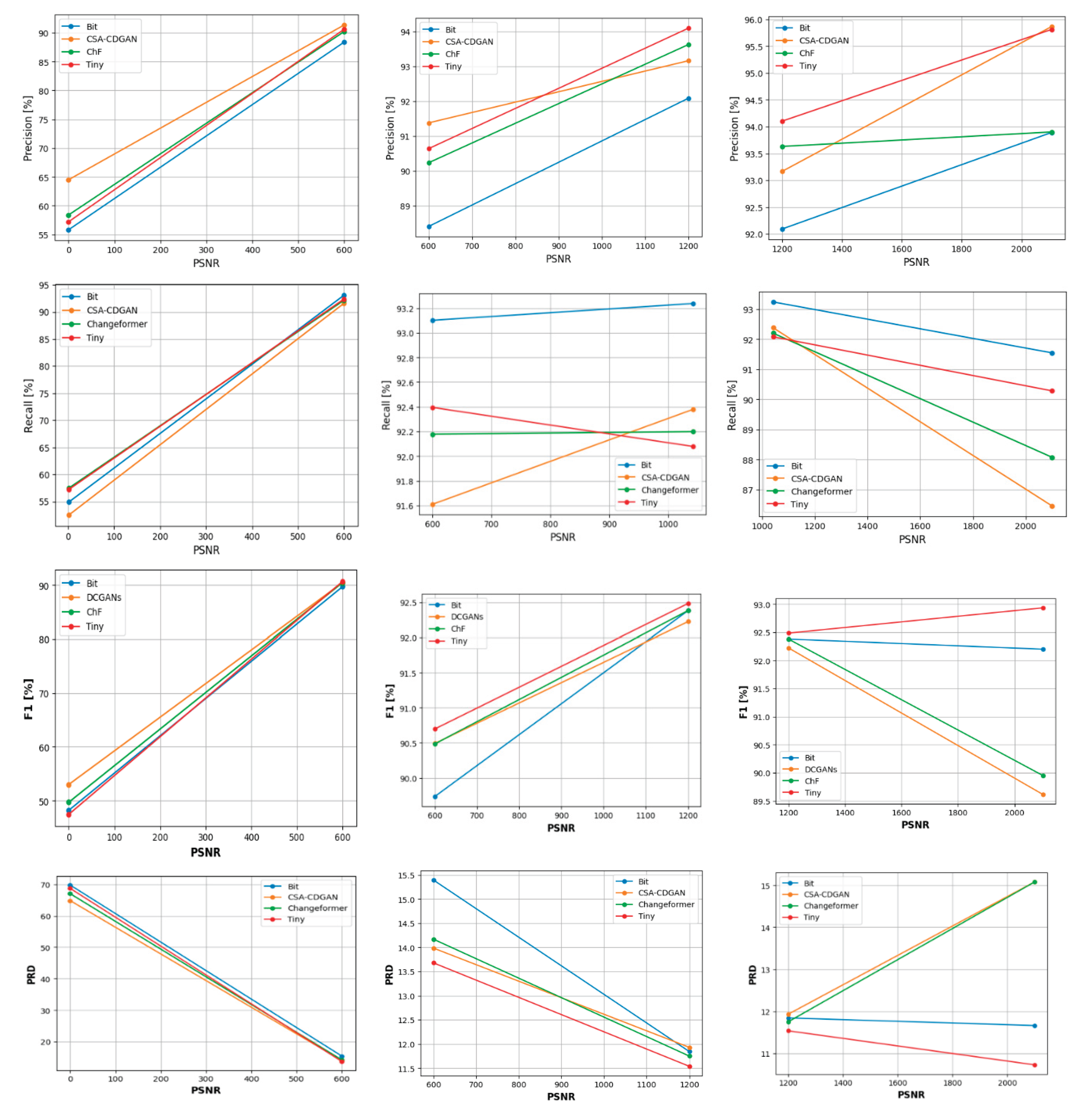
References
- A. Asokan and J. Anitha, “Change detection techniques for remote sensing applications: a survey,” Earth Science Informatics. Springer Verlag, 2019. [CrossRef]
- Institute of Electrical and Electronics Engineers. and IEEE Geoscience and Remote Sensing Society., 2010 IEEE International Geoscience & Remote Sensing Symposium: proceedings, July 25-30, 2010, Honolulu, Hawaii, U.S.A. IEEE, 2010. 25 July.
- H. Chen and Z. Shi, “A spatial-temporal attention-based method and a new dataset for remote sensing image change detection,” Remote Sens (Basel), vol. 12, no. 10, May 2020. [CrossRef]
- A. M. El-Zeiny and H. A. Effat, “Environmental monitoring of spatiotemporal change in land use/land cover and its impact on land surface temperature in El-Fayoum governorate, Egypt,” Remote Sens Appl, vol. 8, pp. 266–277, Nov. 2017. [CrossRef]
- P. P. de Bem, O. A. de Carvalho, R. F. Guimarães, and R. A. T. Gomes, “Change detection of deforestation in the brazilian amazon using landsat data and convolutional neural networks,” Remote Sens (Basel), vol. 12, no. 6, Mar. 2020. [CrossRef]
- 6. L. Ke, Y. Lin, Z. Zeng, L. Zhang, and L. Meng, “Adaptive Change Detection with Significance Test,” IEEE Access, vol. 6, pp. 27442–27450, Feb. 2018. [CrossRef]
- L. T. Luppino, F. M. Bianchi, G. Moser, and S. N. Anfinsen, “Unsupervised Image Regression for Heterogeneous Change Detection,” Sep. 2019. [CrossRef]
- S. Liu, L. Bruzzone, F. Bovolo, M. Zanetti, and P. Du, “Sequential spectral change vector analysis for iteratively discovering and detecting multiple changes in hyperspectral images,” IEEE Transactions on Geoscience and Remote Sensing, vol. 53, no. 8, pp. 4363–4378, Aug. 2015. [CrossRef]
- R. D. Johnson and E. S. Kasischke, “Change vector analysis: A technique for the multispectral monitoring of land cover and condition,” Int J Remote Sens, vol. 19, no. 3, pp. 411–426, 1998. [CrossRef]
- T. Celik, “Unsupervised change detection in satellite images using principal component analysis and κ-means clustering,” IEEE Geoscience and Remote Sensing Letters, vol. 6, no. 4, pp. 772–776, Oct. 2009. [CrossRef]
- Massarelli, “Fast detection of significantly transformed areas due to illegal waste burial with a procedure applicable to landsat images,” Int J Remote Sens, vol. 39, no. 3, pp. 754–769, Feb. 2018. [CrossRef]
- R. Vázquez-Jiménez, R. Romero-Calcerrada, C. J. Novillo, R. N. Ramos-Bernal, and P. Arrogante-Funes, “Applying the chi-square transformation and automatic secant thresholding to Landsat imagery as unsupervised change detection methods,” J Appl Remote Sens, vol. 11, no. 1, p. 016016, Feb. 2017. [CrossRef]
- R. A. A. Raja, V. Anand, A. S. Kumar, S. Maithani, and V. A. Kumar, “Wavelet Based Post Classification Change Detection Technique for Urban Growth Monitoring,” Journal of the Indian Society of Remote Sensing, vol. 41, no. 1, pp. 35–43, Mar. 2013. [CrossRef]
- S. S. Luque, “Evaluating temporal changes using Multi-Spectral Scanner and Thematic Mapper data on the landscape of a natural reserve: the New Jersey Pine Barrens, a case study,” 2000. [Online]. Available: http://www.tandf.co.uk/journals.
- S. J. Kristof, D. K. Scholz, P. E. Anuta, and S. A. Momin, “R. A. WEISMILLER Change Detection in Coastal Zone Environments* Four techniques were used to analyze Landsat MSS temporal data in order to detect areas of change of the Matagorda Bay region of Texas.
- J. Prendes, M. Chabert, F. Pascal, A. Giros, and J. Y. Tourneret, “A new multivariate statistical model for change detection in images acquired by homogeneous and heterogeneous sensors,” IEEE Transactions on Image Processing, vol. 24, no. 3, pp. 799–812, Mar. 2015. [CrossRef]
- E. Kalinicheva, Di. Ienco, J. Sublime, and M. Trocan, “Unsupervised Change Detection Analysis in Satellite Image Time Series Using Deep Learning Combined with Graph-Based Approaches,” IEEE J Sel Top Appl Earth Obs Remote Sens, vol. 13, pp. 1450–1466, 2020. [CrossRef]
- S. De, D. Pirrone, F. Bovolo, L. Bruzzone, and A. Bhattacharya, “A NOVEL CHANGE DETECTION FRAMEWORK BASED ON DEEP LEARNING FOR THE ANALYSIS OF MULTI-TEMPORAL POLARIMETRIC SAR IMAGES.
- IEEE Computational Intelligence Society, International Neural Network Society, Institute of Electrical and Electronics Engineers, and B. C.) IEEE World Congress on Computational Intelligence (2016: Vancouver, 2016 International Joint Conference on Neural Networks (IJCNN): 24–29 July 2016, Vancouver, Canada.
- G. Liu, L. Li, L. Jiao, Y. Dong, and X. Li, “Stacked Fisher autoencoder for SAR change detection,” Pattern Recognit, vol. 96, Dec. 2019. [CrossRef]
- J. Fan, K. Lin, and M. Han, “A Novel Joint Change Detection Approach Based on Weight-Clustering Sparse Autoencoders,” IEEE J Sel Top Appl Earth Obs Remote Sens, vol. 12, no. 2, pp. 685–699, Feb. 2019. [CrossRef]
- J. Liu, M. Gong, K. Qin, and P. Zhang, “A Deep Convolutional Coupling Network for Change Detection Based on Heterogeneous Optical and Radar Images,” IEEE Trans Neural Netw Learn Syst, vol. 29, no. 3, pp. 545–559, Mar. 2018. [CrossRef]
- R. C. Daudt, B. Le Saux, and A. Boulch, “Fully Convolutional Siamese Networks for Change Detection,” Oct. 2018, [Online]. Available: http://arxiv.org/abs/1810.08462. 0846.
- M. Gong, J. Zhao, J. Liu, Q. Miao, and L. Jiao, “Change Detection in Synthetic Aperture Radar Images Based on Deep Neural Networks,” IEEE Trans Neural Netw Learn Syst, vol. 27, no. 1, pp. 125–138, Jan. 2016. [CrossRef]
- K. L. de Jong and A. S. Bosman, “Unsupervised Change Detection in Satellite Images Using Convolutional Neural Networks,” Dec. 2018, [Online]. Available: http://arxiv.org/abs/1812.05815. 0581.
- H. Chen, C. Wu, B. Du, L. Zhang, and L. Wang, “Change Detection in Multisource VHR Images via Deep Siamese Convolutional Multiple-Layers Recurrent Neural Network,” IEEE Transactions on Geoscience and Remote Sensing, vol. 58, no. 4, pp. 2848–2864, Apr. 2020. [CrossRef]
- H. Lyu, H. Lu, and L. Mou, “Learning a transferable change rule from a recurrent neural network for land cover change detection,” Remote Sens (Basel), vol. 8, no. 6, 2016. [CrossRef]
- Institute of Electrical and Electronics Engineers and IEEE Geoscience and Remote Sensing Society, 2019 IEEE International Geoscience & Remote Sensing Symposium: proceedings: July 28–August 2, 2019, Yokohama, Japan. 28 July.
- Hou, Q., Liu, H. Wang, and Y. Wang, “From W-Net to CDGAN: Bi-temporal Change Detection via Deep Learning Techniques,” Mar. 2020. [CrossRef]
- Ren, X., Wang, J. Gao, and H. Chen, “Unsupervised Change Detection in Satellite Images with Generative Adversarial Network,” Sep. 2020. [CrossRef]
- M. A. Lebedev, Y. V. Vizilter, O. V. Vygolov, V. A. Knyaz, and A. Y. Rubis, “Change detection in remote sensing images using conditional adversarial networks,” in International Archives of the Photogrammetry, Remote Sensing and Spatial Information Sciences - ISPRS Archives, International Society for Photogrammetry and Remote Sensing, 18, pp. 565–571. 20 May. [CrossRef]
- Chen, M. Jiang, S. Du, B. Xu, and J. Wang, “ADS-Net:An Attention-Based deeply supervised network for remote sensing image change detection,” International Journal of Applied Earth Observation and Geoinformation, vol. 101, Sep. 2021. [CrossRef]
- J. Chen et al., “DASNet: Dual Attentive Fully Convolutional Siamese Networks for Change Detection in High-Resolution Satellite Images,” IEEE J Sel Top Appl Earth Obs Remote Sens, vol. 14, pp. 1194–1206, 2021. [CrossRef]
- H. Jiang, X. Hu, K. Li, J. Zhang, J. Gong, and M. Zhang, “PGA-SiamNet: Pyramid feature-based attention-guided siamese network for remote sensing orthoimagery building change detection,” Remote Sens (Basel), vol. 12, no. 3, Feb. 2020. [CrossRef]
- Z. Wang, F. Jiang, T. Liu, F. Xie, and P. Li, “Attention-based spatial and spectral network with PCA-guided self-supervised feature extraction for change detection in hyperspectral images,” Remote Sens (Basel), vol. 13, no. 23, Dec. 2021. [CrossRef]
- H. Chen, Z. Qi, and Z. Shi, “Remote Sensing Image Change Detection with Transformers,” Feb. 2021. [CrossRef]
- T. Yan, Z. Wan, and P. Zhang, “Fully Transformer Network for Change Detection of Remote Sensing Images,” Oct. 2022, [Online]. Available: http://arxiv.org/abs/2210. 0075.
- Q. Ke and P. Zhang, “Hybrid-TransCD: A Hybrid Transformer Remote Sensing Image Change Detection Network via Token Aggregation,” ISPRS Int J Geoinf, vol. 11, no. 4, Apr. 2022. [CrossRef]
- T. Lei et al., “Lightweight Structure-aware Transformer Network for VHR Remote Sensing Image Change Detection,” Jun. 2023, [Online]. Available: http://arxiv.org/abs/2306. 0198.
- X. Zhang, S. Tian, G. Wang, H. Zhou, and L. Jiao, “DiffUCD:Unsupervised Hyperspectral Image Change Detection with Semantic Correlation Diffusion Model,” 23, [Online]. Available: http://arxiv.org/abs/2305. 20 May 1241.
- W. G. C. Bandara, N. G. Nair, and V. M. Patel, “DDPM-CD: Remote Sensing Change Detection using Denoising Diffusion Probabilistic Models,” Jun. 2022, [Online]. Available: http://arxiv.org/abs/2206. 1189.
- Y. Wen, X. Ma, X. Zhang, and M.-O. Pun, “GCD-DDPM: A Generative Change Detection Model Based on Difference-Feature Guided DDPM,” Jun. 2023, [Online]. Available: http://arxiv.org/abs/2306. 0342.
- H. Chen and Z. Shi, “A spatial-temporal attention-based method and a new dataset for remote sensing image change detection,” Remote Sens (Basel), vol. 12, no. 10, 20. 20 May. [CrossRef]
- S. Ji, S. Wei, and M. Lu, “Fully Convolutional Networks for Multisource Building Extraction from an Open Aerial and Satellite Imagery Data Set,” IEEE Transactions on Geoscience and Remote Sensing, vol. 57, no. 1, pp. 574–586, Jan. 2019. [CrossRef]
- L. Shen et al., “S2Looking: A Satellite Side-Looking Dataset for Building Change Detection,” Jul. 2021. [CrossRef]
- M. A. Lebedev, Y. V. Vizilter, O. V. Vygolov, V. A. Knyaz, and A. Y. Rubis, “Change detection in remote sensing images using conditional adversarial networks,” in International Archives of the Photogrammetry, Remote Sensing and Spatial Information Sciences - ISPRS Archives, International Society for Photogrammetry and Remote Sensing, 18, pp. 565–571. 20 May. [CrossRef]
- M. Liu, Z. Chai, H. Deng, and R. Liu, “A CNN-Transformer Network With Multiscale Context Aggregation for Fine-Grained Cropland Change Detection,” IEEE J Sel Top Appl Earth Obs Remote Sens, vol. 15, pp. 4297–4306, 2022. [CrossRef]
- H. Chen, Z. Qi, and Z. Shi, “Remote Sensing Image Change Detection with Transformers,” Feb. 2021. [CrossRef]
- S. Fang, K. Li, J. Shao, and Z. Li, “SNUNet-CD: A Densely Connected Siamese Network for Change Detection of VHR Images,” IEEE Geoscience and Remote Sensing Letters, vol. 19, 2022. [CrossRef]
- W. G. C. Bandara and V. M. Patel, “A Transformer-Based Siamese Network for Change Detection,” Jan. 2022, [Online]. Available: http://arxiv.org/abs/2201. 0129.
- Codegoni, G., Lombardi, and A. Ferrari, “TINYCD: A (Not So) Deep Learning Model For Change Detection,” Jul. 2022, [Online]. Available: http://arxiv.org/abs/2207. 1315.
- Z. Wang, Y. Zhang, L. Luo, and N. Wang, “CSA-CDGAN: channel self-attention-based generative adversarial network for change detection of remote sensing images,” Neural Comput Appl, vol. 34, no. 24, pp. 21999–22013, Dec. 2022. [CrossRef]
- Cheng, G., Huang, Y., Li, X., Lyu, S., Xu, Z., Zhao, Q. and Xiang, S., 2023. Change detection methods for remote sensing in the last decade: A comprehensive review. arXiv preprint arXiv:2305.05813, arXiv:2305.05813.
- Parelius, Eleonora Jonasova. "A review of deep-learning methods for change detection in multispectral remote sensing images." Remote Sensing 15, no. 8 (2023): 2092.
- Barkur, Rahasya, Devishi Suresh, Shyam Lal, C. Sudhakar Reddy, and P. G. Diwakar. "Rscdnet: A robust deep learning architecture for change detection from bi-temporal high resolution remote sensing images." IEEE Transactions on Emerging Topics in Computational Intelligence 7, no. 2 (2022): 537-551.
- Paul, Josephina. "Change Detection by Deep Learning Models." In 2022 IEEE International Women in Engineering (WIE) Conference on Electrical and Computer Engineering (WIECON-ECE), pp. 323-326. IEEE, 2022.
- Walatkiewicz, Jonathan, and Omar Darwish. "A Survey on Drone Cybersecurity and the Application of Machine Learning on Threat Emergence." In International Conference on Advances in Computing Research, pp. 523-532. Cham: Springer Nature Switzerland, 2023.
- Abdelsalam, Emad, Omar Darwish, Ola Karajeh, Fares Almomani, Dirar Darweesh, Sanad Kiswani, Abdullah Omar, and Malek Alkisrawi. "A classifier to detect best mode for Solar Chimney Power Plant system." Renewable Energy 197 (2022): 244-256.
- Darwish, Omar, Ala Al-Fuqaha, Muhammad Anan, and Nidal Nasser. "The role of hierarchical entropy analysis in the detection and time-scale determination of covert timing channels." In 2015 International Wireless Communications and Mobile Computing Conference (IWCMC), pp. 153-159. IEEE, 2015.
- Alshattnawi, Sawsan, and Anas MR AlSobeh. "A cloud-based IoT smart water distribution framework utilising BIP component: Jordan as a model." International Journal of Cloud Computing 13, no. 1 (2024): 25-41.
- AlSobeh, Anas. "OSM: Leveraging Model Checking for Observing Dynamic behaviors in Aspect-Oriented Applications." Online Journal of Communication and Media Technologies, 13, no. 4. (2023) pp. 1-18. Cham: Springer Nature Switzerland, 2023.
- Alsobeh, Anas, and Amani Shatnawi. "Integrating data-driven security, model checking, and self-adaptation for IoT systems using BIP components: A conceptual proposal model." In International Conference on Advances in Computing Research, pp. 533-549. Cham: Springer Nature Switzerland, 2023.
- Alsobeh, Anas MR, Aws Abed Al Raheem Magableh, and Emad M. AlSukhni. "Runtime reusable weaving model for cloud services using aspect-oriented programming: the security-related aspect." International Journal of Web Services Research (IJWSR) 15, no. 1 (2018): 71-88.
Figure 1.
Change Detection Methods.
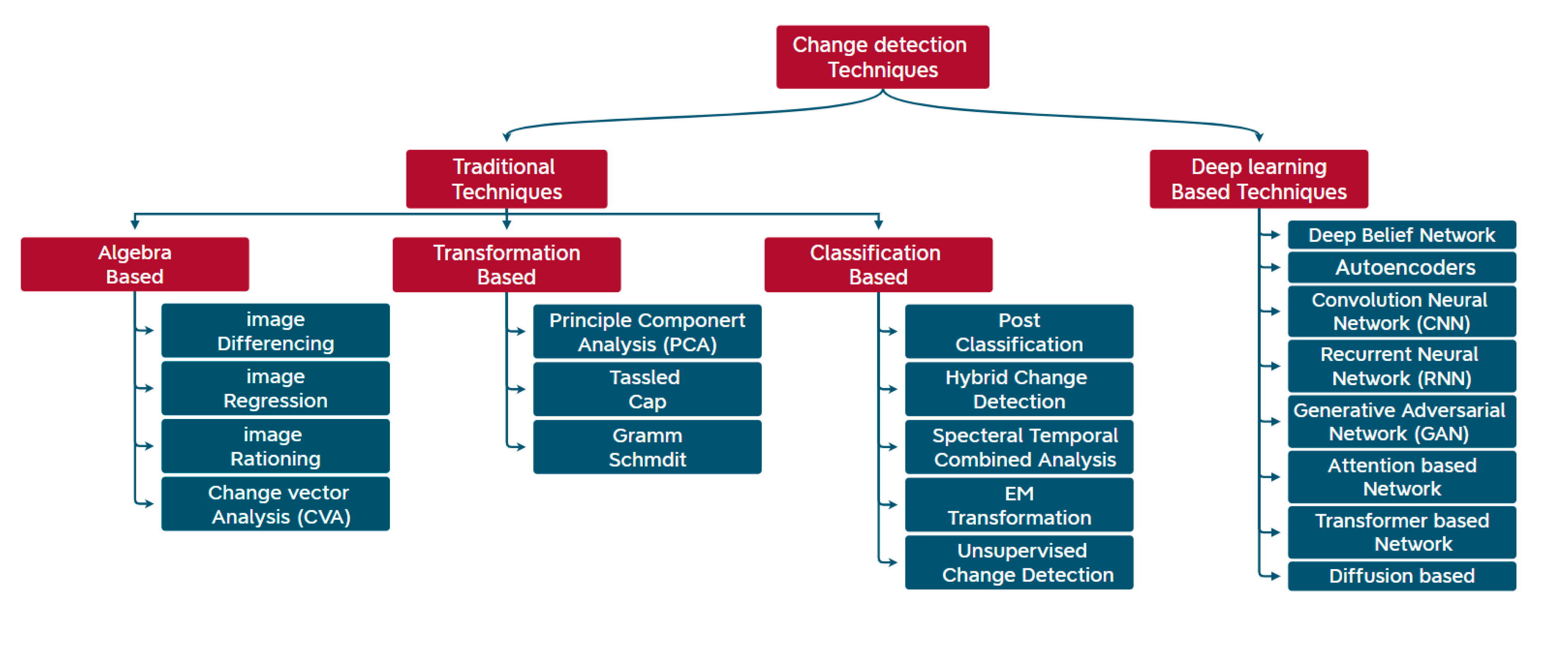
Figure 2.
The flow chart of the proposed Framework.
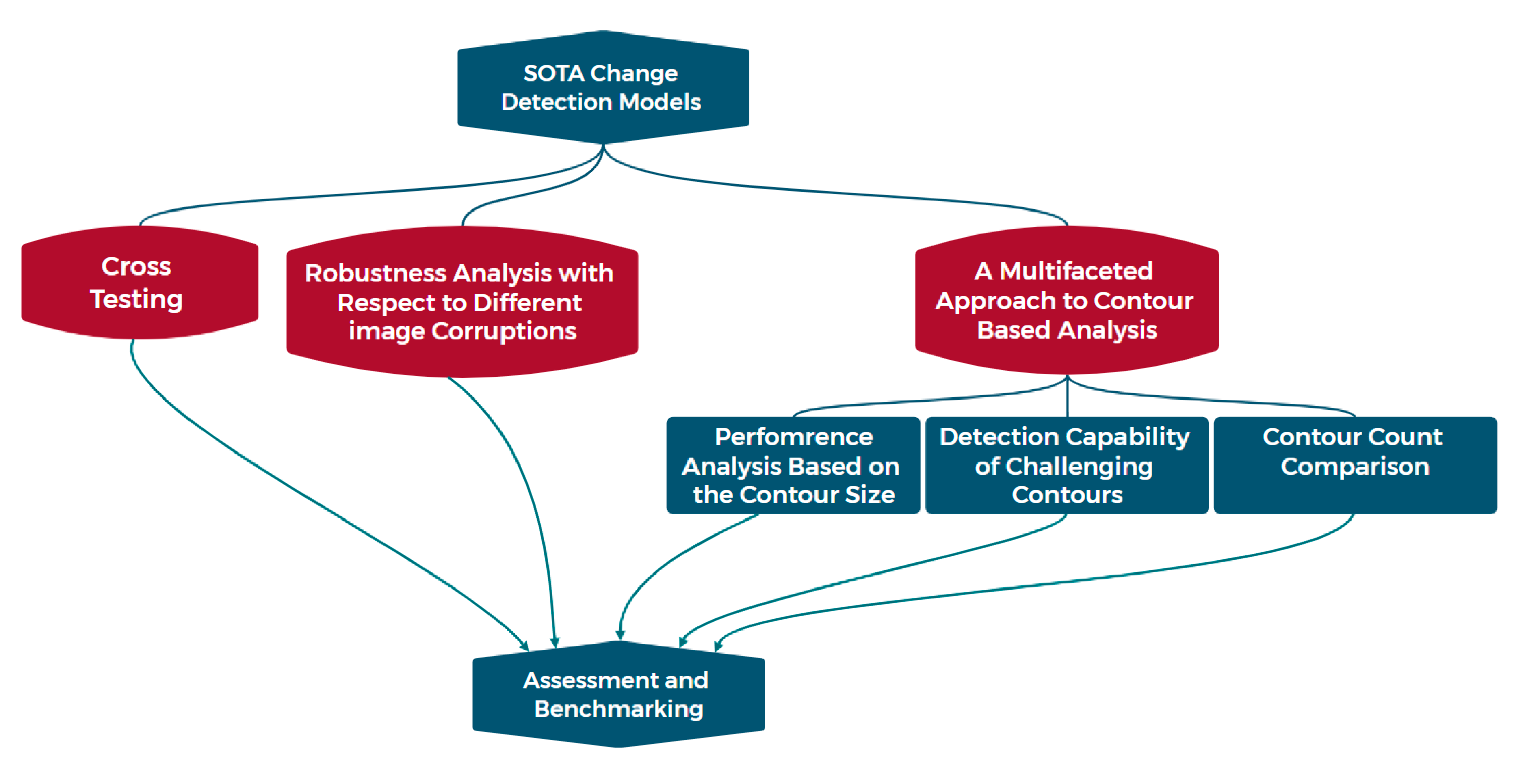
Figure 15.
illustrates the performance of CD models based on different evaluation metrics across various PSNR ranges.
Figure 15.
illustrates the performance of CD models based on different evaluation metrics across various PSNR ranges.
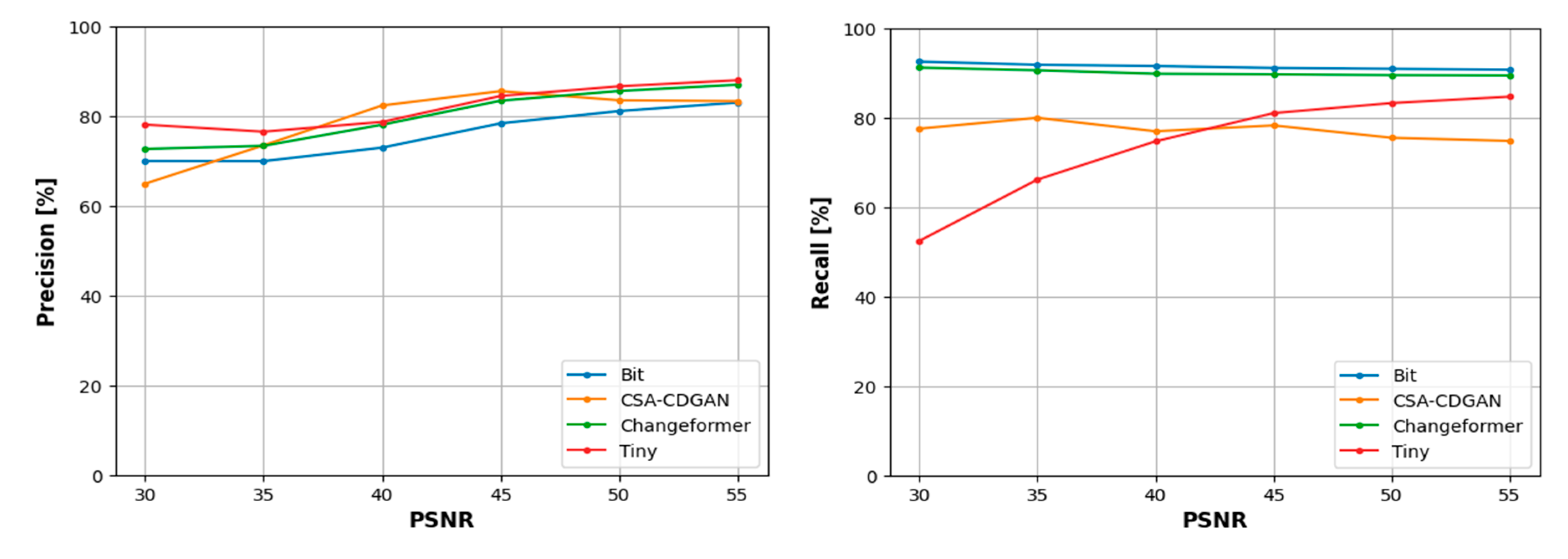
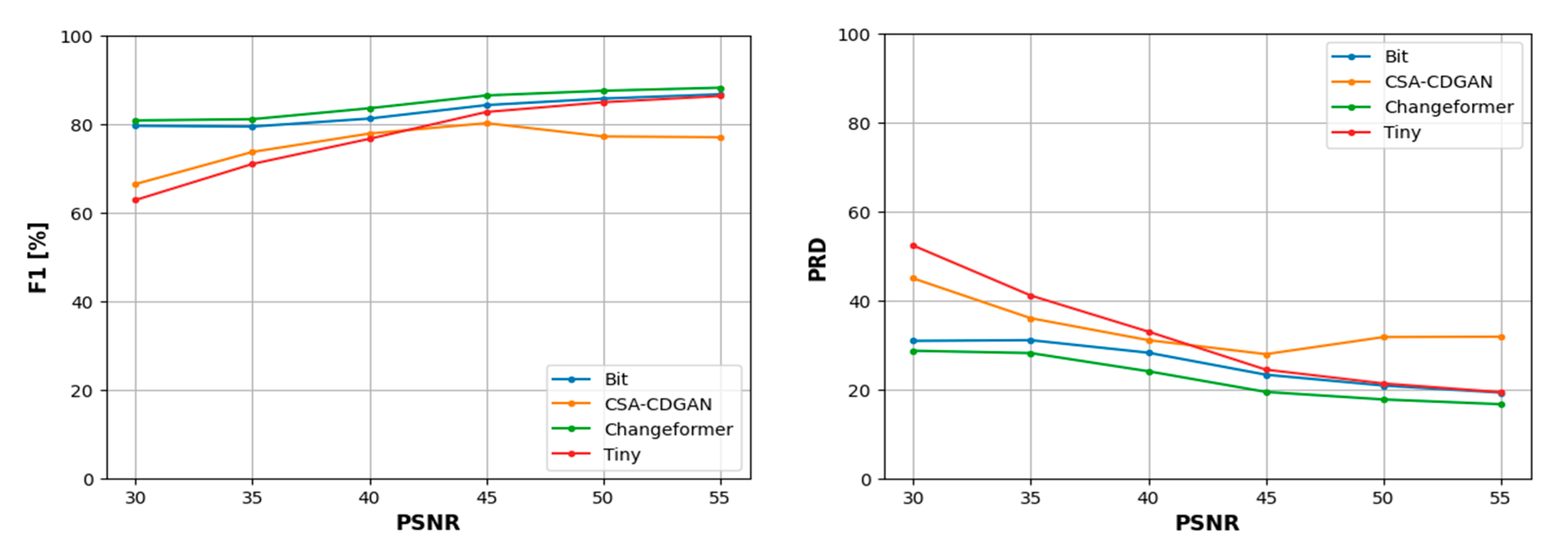
Figure 16.
Samples of the LEVIR testing dataset with Speckle Noise.
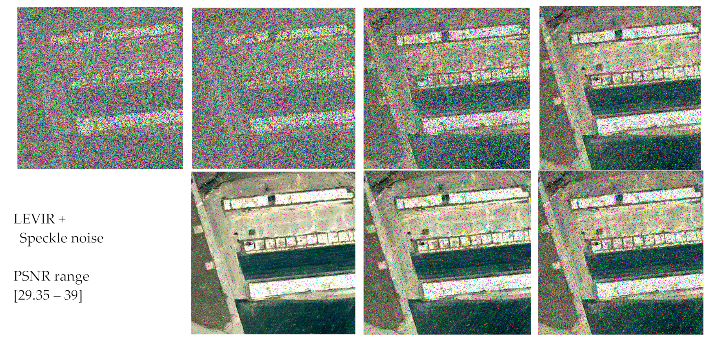
Table 1.
Descriptive statistics of the testing dataset.
| Parameter | Count | Mean | Std | Min | 25% | 50% | 75% | Max |
|---|---|---|---|---|---|---|---|---|
| Size of contour (pixels) | 1682 | 769 | 435 | 2 | 479 | 756 | 1039 | 2086 |
Table 2.
The categorization of the change sizes based on the number of pixels of the changed contour.
Table 2.
The categorization of the change sizes based on the number of pixels of the changed contour.
| Changed Contour Size | Number of Pixels |
|---|---|
| Small | 0 - 600 |
| Medium | 600 - 1200 |
| Large | 1200 - 2100 |
Table 3.
Description of the three noisy datasets.
| Noisy dataset | Number of instances | Range of PSNR (dB) |
|---|---|---|
| Gaussian LEVIR | 2919 | 5 – 35 |
| salt–pepper LEVIR | 1849 | 30 – 55 |
| speckle LEVIR | 6179 | 30 – 35 |
Table 4.
Baseline results on the original LEVIR sample dataset.
| CD model | F1 | Precision | Recall | PRD |
|---|---|---|---|---|
| Tiny | 85.17 | 89.06 | 82.79 | 20.67 |
| Changeformer | 85.36 | 90.18 | 82.54 | 20.28 |
| CSA-CDGAN | 78.45 | 84.00 | 76.29 | 30.30 |
| BIT | 85.14 | 87.17 | 84.06 | 20.78 |
Table 5.
shows the CD model’s performance on the Gaussian LEVIR.
| CD model | F1 | Precision | Recall | PRD |
|---|---|---|---|---|
| Tiny | 83.3 | 77.82 | 89.76 | 24.5 |
| Changeformer | 87.25 | 85.21 | 89.5 | 18.28 |
| CSA-CDGAN | 76.53 | 79.96 | 77.67 | 32.59 |
| Bit | 84.27 | 78.67 | 90.86 | 23.28 |
Table 6.
Drop in performance after adding Gaussian noise.
| CD model | F1 | Precision | Recall | PRD |
|---|---|---|---|---|
| Tiny | -1.87 | -11.24 | 6.97 | 3.83 |
| Changeformer | 1.89 | -4.97 | 6.96 | -2 |
| CSA-CDGAN | -1.92 | -4.04 | 1.38 | 2.29 |
| BIT | -0.87 | -8.5 | 6.8 | 2.5 |
Table 8.
Drop in performance after adding salt & pepper noise.
| CD model | F1 | Precision | Recall | PRD |
|---|---|---|---|---|
| Tiny | -7.09 | -6.86 | -8.04 | 10.37 |
| Changeformer | -0.6 | -9.89 | 7.48 | 1.99 |
| CSA-CDGAN | -2.72 | -4.63 | 0.74 | 3.27 |
| Bit | -2.23 | -11.16 | 7.39 | 4.77 |
Table 9.
shows the CD model’s performance metrics on the speckle LEVIR dataset.
| CD model | F1 | Precision | Recall | PRD |
|---|---|---|---|---|
| Tiny | 74.46 | 63.85 | 89.5 | 37.66 |
| Changeformer | 75.54 | 66.14 | 88.26 | 35.86 |
| CSA-CDGAN | 72.12 | 70.3 | 82.83 | 37.32 |
| Bit | 74.6 | 63.52 | 90.56 | 37.69 |
Disclaimer/Publisher’s Note: The statements, opinions and data contained in all publications are solely those of the individual author(s) and contributor(s) and not of MDPI and/or the editor(s). MDPI and/or the editor(s) disclaim responsibility for any injury to people or property resulting from any ideas, methods, instructions or products referred to in the content. |
© 2024 by the authors. Licensee MDPI, Basel, Switzerland. This article is an open access article distributed under the terms and conditions of the Creative Commons Attribution (CC BY) license (http://creativecommons.org/licenses/by/4.0/).
Copyright: This open access article is published under a Creative Commons CC BY 4.0 license, which permit the free download, distribution, and reuse, provided that the author and preprint are cited in any reuse.


