
Submitted:
18 March 2024
Posted:
19 March 2024
You are already at the latest version
Abstract
In this work, satellite data from the Clouds and Earth’s Radiant Energy System (CERES) and Moderate Resolution Imaging Spectroradiometer (MODIS) instruments is analyzed to determine how the global absorbed sunlight and global entropy generation rate have changed during the time period from 2002 to 2023. The data is used to test hypotheses derived from the Maximum Power Principle (MPP) and Maximum Entropy Production Principle (MEP) about the evolution of earth’s surface and atmosphere. The results indicate that the amount of absorbed sunlight has increased over the last 20 years but rising surface temperatures have caused the entropy generation rate to remain approximately constant despite that decrease in albedo. The results are simpler to explain using the MPP but do not completely rule out the MEP. Given the acceptance of the MPP or MEP, some extensions and nuances are discussed.
Keywords:
Nonequilibrium Thermodynamics
; Life
; Ecosystems
; Evolution
; Entropy Generation
; Geoengineering
; Social Sciences
; Albedo
; Externalities
1. Introduction
The idea that earth is regulated by life for life rings true. Beyond the impact of humans on the environment,[1] early prehistoric photosynthetic organisms are believed to have changed the composition of the atmosphere to be oxygen rich.[2] Since then, global photosynthesis has maintained the chemical composition of the atmosphere far away from the local equilibrium state at the surface temperature and pressure of the earth.[3] Even more remarkable is that this nonequilibrium chemical composition is relatively stable over time periods much longer than the average CO2 residence time on the atmosphere,[4] which is on the order hundreds of years.[5] Such behavior resulting in a relatively stable, albeit unexpected chemical state suggests amenability to thermodynamic analysis. The penultimate goal of such an analysis would be to understand what controls the stationary state(s) towards which the earth is trending, and thereby make probabilistic forecasts.
Principles have been proposed that govern systems that operate over long periods of time very far from local equilibrium, such as life itself. Building on phenomenological observations of ecosystems, the Maximum Power Principle (MPP) is an often-cited example of a principle that governs evolution of complex communities containing living organisms. The development of the MPP has been lucidly described in a recent work by Hall and McWhirter,[6] and so it will not be repeated here. In brief, the basic idea is that ecosystems evolve, subject to external constraints (e.g. element availability, energy source, etc.), towards stationary states that maximize the flow of energy through the ecosystem per unit time, which is power. There is a related idea that was popularized most recently in a series of papers by Kleidon[7,8,9,10,11,12] and others[13,14,15,16] that is termed the Maximum Entropy Production Principle (MEP). The MEP hypothesis basically states that the ecosystem will evolve towards a state where it generates the most entropy per unit time from an external energy flow. The MPP and MEP hypotheses are related. For example, if an ecosystem survives on the flow of heat between two reservoirs that have constant temperatures, then at steady-state the entropy generation rate is proportional to the energy flow by the difference in reciprocal temperatures of the reservoirs. For such an ecosystem driven by a flow of heat between two isothermal reservoirs, MPP and MEP are the same. If, however, the temperatures of one or both of the reservoirs can change, then the situation becomes more complicated, and the different principles may predict different trajectories.
The goal of this work is to test the MPP and MEP hypotheses, or at least evaluate them given state of the art information. The first step of a thermodynamic analysis is defining the system boundary and the exchanges of matter, energy, and entropy across that boundary. It is relatively straightforward to draw a boundary around an ecosystem, but describing the exchanges of matter, energy and entropy across that boundary is exceedingly difficult for most subsystems on earth. However, the situation can be simplified if the entire earth is taken as the ecosystem. The earth is nominally a closed system. The matter that crosses the top of the atmosphere[17,18] is negligible compared to the amount of matter contained within the system. Furthermore, the exchanges of energy and entropy across the boundary are dominated by several orders of magnitude by radiation.[9] There are only three main external exchanges between the earth and outer space: 1) shortwave (SW) radiation input from the sun in the visible and near infrared regions of the electromagnetic spectrum, 2) SW radiation output that is sunlight scattered from the surface and atmosphere (e.g. clouds) in the visible and near infrared regions of the spectrum, and 3) longwave (LW) thermal radiation in the infrared with a spectrum determined by the temperature of the earth surface and clouds being in the range from 210 to 325 K. These radiation energy exchanges, when time-averaged and integrated over the entire surface of the earth, are on the order 104 to 105 terawatts (TW), several orders of magnitude higher than the next closest energy exchanges. Geothermal heat via volcanic activity coming from the earth core and radioactive decay, as well as global combustion by human fossil energy utilization, only amount to approximately 101 to 102 TW on average.[9] Since the other exchanges are insignificant, the system is adequately described by only the three radiation exchanges, and from those exchanges, the energy flow through the earth and the entropy production rate by the earth can be quantified.
Both the MPP and MEP principles predict evolution towards an extremum. More specifically, a stationary state whereat the energy flow through the earth is maximized in the case of MPP, or entropy production rate by the earth is maximized in the case of MEP. Energy flow through the earth is taken to be the amount of absorbed sunlight since the earth is nominally in steady state and the net energy absorbed at SW wavelengths is balanced by energy outflow at LW wavelengths. The expectation for both MPP and MEP is that the corresponding variable (energy flow or entropy generation rate) will either increase in time (heading towards a maximum) or remain constant (already at the maximum). Since the temperature of the earth is changing due to global warming, and the albedo of the earth has changed over the last several decades,[19] analysis of recent global trends as characterized by satellite measurements may allow for discrimination between the MPP and MEP hypotheses.
In this work, recently reported satellite measurements of the power density of 1) incoming SW solar radiation, 2) outgoing SW radiation and 3) outgoing LW radiation from earth were combined with satellite measurements of 4) cloud cover area fraction, 5) cloud temperature, 6) sea temperature and 7) day/night land temperatures to estimate how the absorbed sunlight and net global entropy exchange with space has changed over the period from the year 2002 to 2023. The key findings are that 1) the absorbed sunlight has increased from 2002 to 2023, corroborating recent reports that the albedo has decreased,[19] and 2) the entropy generation rate has remained approximately constant. In other words, rising global surface temperature from the greenhouse effect compensated for the rising amount of absorbed sunlight to keep the entropy generation rate of earth approximately constant. The results tend to support the MPP over the MEP hypothesis, but do not rule out MEP. The conclusion is that observations made of global temperature distributions and energy fluxes over the last two decades are consistent with both the MPP and MEP hypotheses governing the global ecosystem, including human society. While we cannot rule out either hypothesis completely, it is a notable result that recent satellite measurements are consistent with these hypotheses being true.
2. Materials and Methods
This research was an analysis of satellite data that has been publicly reported by the United States National Aeronautics and Space Administration (NASA). The time period studied was from July 2002 to August 2023 inclusive. The data was spaced monthly on a 1o × 1o grid in longitude and latitude. Cloud area fraction, cloud temperature, SW light input, SW light output, and LW light output were all downloaded as a Top of Atmosphere Energy Balanced and Filled (EBAF-TOA) data product from the Clouds and the Earth’s Radiant Energy System (CERES) instrument.[20,21] Day/night land temperatures[22] and sea temperatures[23] were downloaded from the Moderate Resolution Imaging Spectroradiometer (MODIS) datasets. The data was imported using Origin 2019 Pro (OriginLab, North Hampton MA) and then exported to Matlab R2015a (MathWorks, Natick MA) for analysis. Contour plots were made in Origin 2019 Pro.
Data from the MODIS instrument for the day land temperature, night land temperature, and sea temperature were combined to make an effective surface temperature as a function of position (longitude, latitude, and month). If the coordinate was surface water, then the sea temperature was used. If the coordinate was land, then the temperature was time-averaged using the number of daylight hours. In other words, the average land temperature was taken as:
where x is the average number of daylight hours for the location and month divided by the number of hours in the day; and the day and night temperatures have the corresponding subscripts. There were a few holes in the MODIS dataset where no temperatures were reported. Since the surface temperature depends primarily on latitude and month, those data holes were filled with the latitudinal average surface temperature for the corresponding month.
Data from CERES was used without modification. For a given pixel, the radiation exchanges were calculated by multiplying a given energy flux by the area corresponding to the pixel:
Here i is the index of the corresponding energy flux (qi), which depends on position and time (net flux, SW input, SW output or LW output in units of W m-2). The usual definition of longitude (λ) and latitude (φ) has been used and the units of those angles are degrees. The radius of the earth (r) is taken as the average of the polar and equatorial radii (6.367×10⁶ m). Since the data is on a 1o×1o grid, both dφ and dλ are taken as 1o.
The system definition with the corresponding boundary interactions is presented in Figure 1. It was assumed that the entire earth is in steady state, which means that the energy outflow with SW and LW radiation is equal to the SW energy inflow such that there is negligible accumulation of energy within the boundary. The steady state assumption also means that there is no accumulation of entropy within the system, such that the entropy inflow with SW radiation plus the entropy generation is equal to the entropy outflow with SW radiation and LW radiation. The steady state assumption for the energy and entropy exchanges is justified by the fact that any minor imbalances are much smaller than the total internal energy and entropy contained within the surface of the earth and atmosphere.
The energy balance requires integrating the local energy fluxes over the surface of the earth. For a given position as defined by a longitude-latitude pair, the net energy exchange can be written using equation (2):
Here the sunlight input, SW output and LW output are all provided explicitly by the CERES data product as a function of position and time; and the sign convention is positive going in and negative going out (Figure 1). The total energy exchange with space can be calculated by integrating equation (3) over the entire surface of the earth:
where Qnet has units of power (e.g. terawatt, TW). Equation (4) and other equations of similar form were integrated numerically. If the earth is in steady state from an energy accumulation perspective, then equation (4) is expected to be equal to zero. Since all three energy fluxes are provided in the CERES data set, equation (4) can be used to check the steady state assumption that is required in the entropy balance to calculate the entropy generation rate (vide infra).
Similar to the energy balance, the entropy balance requires integrating the fluxes over the entire surface of the earth. There is an entropy exchange with space for each of the energy exchange terms, and so we can write the net entropy exchange in the same way as the energy exchange:
In equation (5), the terms in the bracket correspond to the entropy flux due to the solar input (ssun,in), reflected SW output (sSW,out), and emitted LW thermal radiation output (sLW,out); all of which depend on position and time. The global entropy production rate (GEP) is straightforward to calculate after integration of equation (5) has been performed by doing a steady state entropy balance:
The task now becomes to describe the entropy fluxes from quantities that are known from the MODIS and CERES datasets. Energy fluxes are proportional to entropy fluxes by an effective temperature (Ti):
All of the energy fluxes are known from the CERES dataset, and thus only the corresponding effective temperatures need to be described as a function of space and time.
The easiest of the temperatures is the solar input. Radiation is emitted from the sun with a temperature of approximately 5500 K. As it travels through space, the spectral distribution remains mostly unchanged and similar to a blackbody at the surface temperature of the sun. However, the energy flux decreases with distance from the sun, which causes the spectral temperature of the sunlight, (Tsun,in in equation (7)) to decrease. Expressions that relate entropy flux to the spectral irradiance of a nonequilibrium light source have been known for decades.[24,25,26] The basic idea is that for each wavelength bin, one can find a blackbody temperature that would produce the irradiance at that wavelength, and then calculate the corresponding entropy flux. By summing up the entropy flux contributions of each wavelength bin, the total entropy flux can be calculated for an arbitrary nonequilibrium irradiance spectrum. Performing such a calculation for the AM0 spectrum that describes the sunlight incident upon the top of the atmosphere, the spectral temperature of the solar input can be estimated as approximately Tsun,in = 1200 K, which is notably lower than the surface temperature of the sun.
The dependence of the spectral temperature on energy flux is relatively weak. For example, the irradiance at the surface of the sun estimated using the Stephan-Boltzmann law is approximately 10,000 times higher than at the surface of the earth; and yet the spectral temperature of sunlight at the surface of the sun is only 4.6 time higher. Since the reflected SW light from the earth has an irradiance of approximately 30% of the incident SW sunlight, and the dependence of the spectral temperature on irradiance is relatively weak, it is reasonable to assume that:
in the absence of any detailed spectral irradiance data for the SW output. It is worth noting that if the spectral irradiance of the SW output were known, for example by more sophisticated broadband hyperspectral satellite measurements in the future, then TSW,out or sSW,out could be calculated directly as a function of position and time.
The final effective temperature is associated with the LW thermal emission, TLW,out, which is expected to be in the range of surface and cloud temperatures. Again it is emphasized that if the spectral irradiance of the LW radiation output were known, the entropy flux sLW,out could be explicitly calculated without the need for any approximations involving temperatures reported by the CERES and MODIS instruments. Unfortunately, at present the spectral irradiance of the radiation outputs is not known with sufficient spectral and spatial resolution, and thus simplifying approximations must be made to use the available data. For each pixel, surface and cloud temperatures are known. Additionally, the CERES data set includes the fraction of the pixel area that is estimated to be covered by clouds.[27] The entropy flux with the LW output from a pixel is calculated by assuming that the LW energy flux is partitioned between the cloud and surface according to the cloud area fraction:
where fcloud is the fraction of the pixel area that is cloud covered, Tcloud is the cloud temperature reported in the CERES dataset, and Tsurf is the sea temperature if the pixel is water, or the land temperature calculated using equation (1) if the pixel is land.
An example of a complete set of temperature data required to calculate the total entropy exchanged with space using equation (5) for one time point is provided in Figure 2. The cloud area fraction is presented in Figure 2a, the cloud temperature in 2b, and the composite surface temperature in Figure 2f with the constituents used to construct that composite in Figures 2c-2e.
The earth has an annual cycle. The planet does not follow a perfect circular orbit with the sun at the middle. In addition to the summer/winter cycle, the earth is closest to the sun during the southern hemisphere summer, which results in a higher global solar input during that time of year. The annual cycle causes a periodic trend in all the global radiation exchanges with space that has a period of 1 year (vide infra). The magnitude of the annual variation is rather large. For example, consider the swing in temperature from summer to winter compared to the magnitude of the temperature change due to global warming. To reveal trends in the underlying energy and entropy fluxes, and associated surface temperatures, it is helpful to compensate for the annual cycle. In this work, the annual cycle is compensated for by considering the value of a variable in a given month (energy flux, entropy flux, temperature, etc.) relative to the value of that variable in the same month of a reference year. More specifically, consider the value of some variable Ki that varies with time and longitude/latitude:
where the overbar denotes a relative value. The superscripts denote that it is a value for month j of year z. The superscript ref denotes the reference year. While the year z may increment through time, the reference year ref is a constant. The reference year chosen for this work is 2003, which is the earliest year for which a complete dataset was available.
3. Results
Since the LW thermal emission is isotropic, but the SW exchanges are not, the net exchange of radiation with space is negative (outgoing) in locations and months of the year where the incoming solar is weak, for example during the winter; and positive (incoming) at locations and months of the year where the sunlight is strong, for example during the summer. To illustrate this important trend, an example map of the net radiation exchange for an arbitrary month (May 2005) is plotted in Figure 3a. From approximately -10o to 60o latitude there was a net absorption of energy, while south and north of this band there was a net emission of energy into space. The band of net radiation absorption and bands of net radiation emission shift throughout the year with the annual cycle.
The earth is approximately in steady state, meaning there is very little accumulation of energy in the control volume over time. Plotted in Figure 3b are the globally integrated solar input, SW output, and LW output as a function of time from 2002 to 2023. The solar input displays an annual cycle according to the distance of the planet from the sun. The net exchange, calculated by summing all three radiation contributions at a given time point via equation (4), oscillates about zero with a very small amplitude and a period of 1 year. Thus, the steady state assumption is reasonable since the net exchange is approximately zero. By compensating for the small variations of the annual cycle using relative values via the approach outlined in equation (10), effects of the tiny oscillations about zero with a period of 1 year can be removed to reveal long term trends.
Applied to the entire planetary ecosystem, the expectation of the MPP is that evolution should occur in such a way that sunlight absorbed by the earth will increase (approaching a maximum) or stay the same (already at the maximum). Assuming steady state, the amount of sunlight absorbed by the earth can be calculated as the globally integrated solar input minus the SW output. The globally absorbed sunlight, so calculated, is plotted in Figure 4a without removing the effect of the annual cycle and in Figure 4b as a relative value calculated using equation (10). Even with data that is uncompensated for the annual cycle (Figure 4a), a trend of increasing maxima and increasing minima can be seen that already shows that the rate at which the earth is absorbing sunlight appears to have increased over this time period. Plotting the same data relative to the year 2003 (Figure 4b), a moving average with a window of 12 months more clearly shows the magnitude by which the amount of absorbed sunlight has increased over the last 20 years – approximately 1000 TW. This trend is consistent with the expectation of MPP.
Over the same time period from 2002 to 2023, the average surface temperature of the earth has increased but the average cloud temperature has remained approximately constant. Plotted in Figure 5a are the area-averaged surface and cloud temperatures without compensating for the annual cycle. The surface temperature is obviously much higher than the cloud temperature, as expected. Plotting the temperatures relative to the same point in the annual cycle of the year 2003 for the surface (Figure 5b) and clouds (5c) more clearly shows that the surface has increased in temperature over the last 20 years but the clouds have stayed approximately the same temperature, which is consistent with the greenhouse effect. While the increased sunlight absorption (Figure 4) played a role in the increasing surface temperature (Figure 5b), it must be noted that the magnitude of the climate forcing due to this decreased albedo is less than the magnitude of the forcing due to the greenhouse effect.[19] Figure 4 and Figure 5 are the crux of the problem for the MEP hypothesis, which has been previously articulated as a criticism.[28] On the one hand, the earth is absorbing an increasing fraction of the incident sunlight (Figure 4), which should tend to increase the global entropy production rate at constant temperature. On the other hand, the global temperature is increasing (Figure 5), which should tend to decrease the global entropy production rate at constant absorbed sunlight. The outcome of the competition between these two countervailing phenomena for the global entropy production rate is not obvious, and the calculation must be done.
Everywhere in the world, at all times examined in the dataset, the net entropy flux was negative, consistent with the 2nd law of thermodynamics, the steady state assumption, and the assumption that radiation comprises the largest energy and entropy exchanges when averaged over a 1o×1o pixel. The more negative is the entropy flux, the higher the local entropy generation rate due to the radiation exchanges. Plotted in Figure 6a and 6c are the net energy flux maps for two arbitrary winter/summer months: January 2005 and July 2005. Plotted in Figure 6b and 6d are the net entropy flux maps for the same months. As expected, the net entropy flux is more negative in the hemisphere experiencing winter because the net energy flux is negative, and the temperature is smaller than the hemisphere experiencing summer. When integrated over the surface, the portion of the world that receives less solar input is the portion of the world that contributes more to the global entropy production rate. The conclusion is visualized as a coincidence between the blue regions of the net energy flux maps (outgoing net energy flux) and the pink regions of the entropy flux maps (most negative net entropy flux), which change with the season but are correlated at a given time point. Integrating maps such as those in Figures 6b and 6d over the entire surface of the earth using equations (5) and (6) provides the global entropy production rate in time.
The global entropy production rate displayed stochastic changes over the last 20 years but remained approximately constant. Plotted in Figure 7a is the global entropy production rate calculated using equations (5) and (6) without compensating for the annual cycle. Contrary to the absorbed sunlight data, it is difficult to see any trend from the maxima and minima of the oscillations. When the global entropy production rate is plotted relative to the year 2003 to compensate for the annual oscillations, fluctuations are observed but there is no long-term trend over the studied time period (Figure 7b). There is a series of large fluctuations in the time period from 2007 to 2014 that are a few years wide on the solid curve (Figure 7b), which is a moving average with a 12 month window. Interestingly, the minima in the global entropy production rate (Figure 7b) during this period correspond to maxima in the absorbed sunlight (Figure 7c) and vice-versa. The behavior may be related to trends in the cloud temperature during the same period (Figure 5c).
The expectation of the MEP is that the global entropy production rate should increase (approaching a maximum) or stay the same (already at a maximum). Kleidon has previously argued that the earth is at a maximum in the global entropy production rate,[8] which the results presented herein appear to be consistent with. If the MEP principle is true and the earth is at a maximum, then increases in the surface temperature must be compensated for by increased absorption of sunlight, which would result in a positive feedback loop.
4. Discussion
The present results are consistent with both the MPP and MEP hypotheses, thus neither can be ruled out completely. However, the MEP is discounted in favor of accepting the MPP hypothesis. The reason is that the surface temperature of the earth is much higher than the steady state blackbody temperature assuming complete absorption of the solar energy input and no greenhouse effect. Therefore, the surface temperature of the earth could, in principle, decrease considerably while still satisfying the 1st and 2nd laws of thermodynamics. Such a decrease in surface temperature would increase the global entropy production rate. Alternatively, the global absorbed sunlight could increase while the surface temperature remains constant, which would also increase the global entropy production rate. And yet, neither of these possible pathways appear to be happening; neither decreased temperature at constant energy flow nor constant temperature with increased energy flow. It is possible that the constraints of the complex living system that is earth, which we do not fully understand, do not allow these pathways towards higher entropy production rate to occur – it cannot be ruled out. However, given these two hypotheses MPP and MEP, it is simpler to explain how the empirical trends (Figure 7) support MPP. Thus, by Occam’s razor, this author leans towards accepting MPP and discounting MEP. The acceptance of MPP would have important consequences for global warming. Currently, approximately 30% of sunlight is reflected from earth as SW radiation. Thus, there is plenty of room to absorb more incident sunlight, and thus we can expect in the future even lower albedo. It makes mitigating the greenhouse effect even more important because increased absorption of incident sunlight means increased cooling capacity will be needed to maintain an acceptable surface temperature for life.
Purpose
To avoid confusion, it is worthwhile to elucidate how the extremum principle, whether it be MPP or MEP, is envisioned being used. First it is necessary to outline different types of thermodynamic systems since the extremum principle only applies to certain types of systems. There are the well-known systems that are governed by local equilibrium, which are the subject of numerous engineering thermodynamics textbooks. These systems tend towards a stationary state that is the equilibrium state constrained by the local state variables, for example temperature and pressure. The equilibrium state is subject to an extremum principle - maximum entropy in an isolated system, which can be cleverly defined to model the problem at hand.[29] There are nonequilibrium systems that are maintained by dissipating an external energy flow, external mass flow, or both. Nonequilibrium systems can be either close to local equilibrium, also known as linear nonequilibrium systems; or they can be far from local equilibrium, also known as nonlinear nonequilibrium systems. There are mathematical inequalities that can be used to determine whether a system is close to, or far away from, local equilibrium. For a clear discussion, see the lucid book of Prigogine and Kondepudi.[30] Lovelock and Margules succinctly pointed out in their seminal work on the Gaia hypothesis that the earth operates perpetually with a chemical composition that is far from local equilibrium, therefore it is in the nonlinear regime. Similar to how entropy maximization is the extremum principle that describes systems governed by local equilibrium; the key idea is that the MPP or MEP act as an extremum principle that governs systems that are constrained to operate far from local equilibrium, such as the surface of the earth, atmosphere, and the life contained within. The extremum principle is expected to be general to systems in the nonlinear regime of thermodynamics. For example, the author has also applied this idea to describe chemical reactions in a different type of system that operates far from local equilibrium, specifically low-temperature plasma reactors.[31,32,33]
Let the term Gaia be used to describe a system with a boundary that contains only the matter on earth that operates perpetually very far from equilibrium in the nonlinear regime of irreversible thermodynamics, which at a minimum includes all life and human society; but is more expansive and includes information technology, artificial intelligence and other material objects of the surface and atmosphere. It is tempting to describe increasing the flow of energy through the earth, or increasing the entropy production rate of the earth, as the purpose of Gaia. However, terms such as purpose, objective, goal, etc.; anthropomorphize a system by implying a choice and the ability to act on that choice when no choice may exist. For example, a hot beverage cup, which is governed by local equilibrium, does not have a choice. In the absence of an energy source with higher temperature, the cup exchanges heat with its environment until the temperatures are equal because that is the natural law it must obey. It is not an anthropomorphic goal, rather Gaia increases the energy flow or entropy production rate because it is governed by a probabilistic natural law described by the MPP or MEP. In other words, systems close to equilibrium are governed by local equilibrium and tend towards equilibrium, while driven nonlinear irreversible systems tend towards maximum power or maximum entropy production. The idea is that if the system within the boundary comprising Gaia is to remain as a nonlinear irreversible system, which is required for it to contain life, then it must, subject to its constraints, probabilistically maximize the power flow through it or its entropy production rate. This all presumes acceptance of MPP or MEP.
Implications for Climate Change Mitigation
At present neither the MPP or MEP can be ruled out, thus the focus will be on global trends that are expected to satisfy both – specifically increasing the fraction of sunlight that is absorbed by the earth. If the MEP principle were true, then the analysis is more nuanced because one must also consider temperature and the difficulties with describing it at a global scale. According to the MPP and arguably MEP, societal trends that increase the amount of globally absorbed sunlight are expected to have a higher probability of occurrence than trends that decrease it. Societal trends are defined here to be concerted efforts of large human populations that have significant impacts on the fraction of incident sunlight absorbed by the earth. The connections between human activity and the absorbed sunlight by the earth are generally complex and difficult to discern. However, in some instances the connections appear to be relatively clear.
Decreasing albedo is generally expected by MPP and also can be expected from MEP depending on how surface temperatures change. Thus, activities focused on decreasing albedo are expected to be probable. An interesting approach to decreasing albedo, specifically surface albedo, is to place very large arrays of solar energy harvesting devices such as photovoltaic solar panels in a desert. Since the purpose of these devices is to generate electricity from sunlight, they are typically designed for maximum absorption and have a much lower surface albedo when compared to the naturally occurring surfaces in deserts. Moreover, deserts are locations of high sunlight intensity, and thus can have a higher impact on the sunlight absorbed by the earth than placing solar energy harvesting devices elsewhere.
From the vantage point presented in this work, geoengineering strategies[34] appear misguided that aim to lower the surface temperature of the earth by increasing the albedo for example using clouds seeded by intentionally introduced aerosols. Increases in albedo are improbable and opposed to the MPP, and probably also MEP, depending on how temperatures change. A concerted effort is unexpected by human society that would cause so much cloud cover that it lowers the surface temperature by reflecting incoming sunlight.
Externalities May Cause Perturbations
There have been periods in the past during which the albedo of the earth has increased abruptly. For example, in the year 1991, the Pinatubo volcano erupted spewing ash into the atmosphere, which caused an immediate increase in albedo[35] and cooling of the atmosphere.[36] Furthermore, prehistorical changes in climate included several transitions from hot-houses to cold-houses,[37] including transitions from warm climates to ice-ages, and the albedo was presumably higher during those ice-ages due to increased snow cover than it was during the preceding warm period. At first glance these transitions appear to contradict MPP and MEP, from which decreasing albedo with time is expected. While prehistorical drivers of these climate changes are difficult to know with certainty, evidence suggests that sudden decreases in global average temperature and the commensurate increase in albedo are correlated with the impacts of very large celestial objects on the surface of the earth, or volcanic eruptions. For example, approximately 66 million years ago, the impact of the bolide that made the Chicxulub crater, which is 150 km in diameter, is believed to have caused the subsequent global average temperature change of approximately -10 oC due to increased albedo from atmospheric aerosol injection.[38] It is remarkable that during the last 540 million years, following excursions to global average temperatures as high as 40 oC and as low as 10 oC; the temperature has apparently repeatedly returned to a relatively stable ~ 20 oC, although it sometimes took 10 million years or more for that stabilization to happen.[37] The observation of damping of the excursions back towards the mean suggests that the causal events originated from outside Gaia, and therefore these events are termed externalities.
Celestial objects obviously originate from outside Gaia and are therefore external to the system that is governed by MPP or MEP. Since bolides are external to Gaia, they can affect the albedo and radiative temperature in a way that decreases the entropy production rate or absorbed sunlight. Following the impact, provided life is not completely extinguished and the earth’s surface and atmosphere remain in the nonlinear regime of irreversible thermodynamics, Gaia is expected to begin again towards the extremum subject to whatever new constraints the externality may have imposed. Thereby the effect of the externality is expected to damp out over long periods of time. In this way, global warming is not a major concern from the perspective of Gaia, although it is a concern from the perspective of human society.
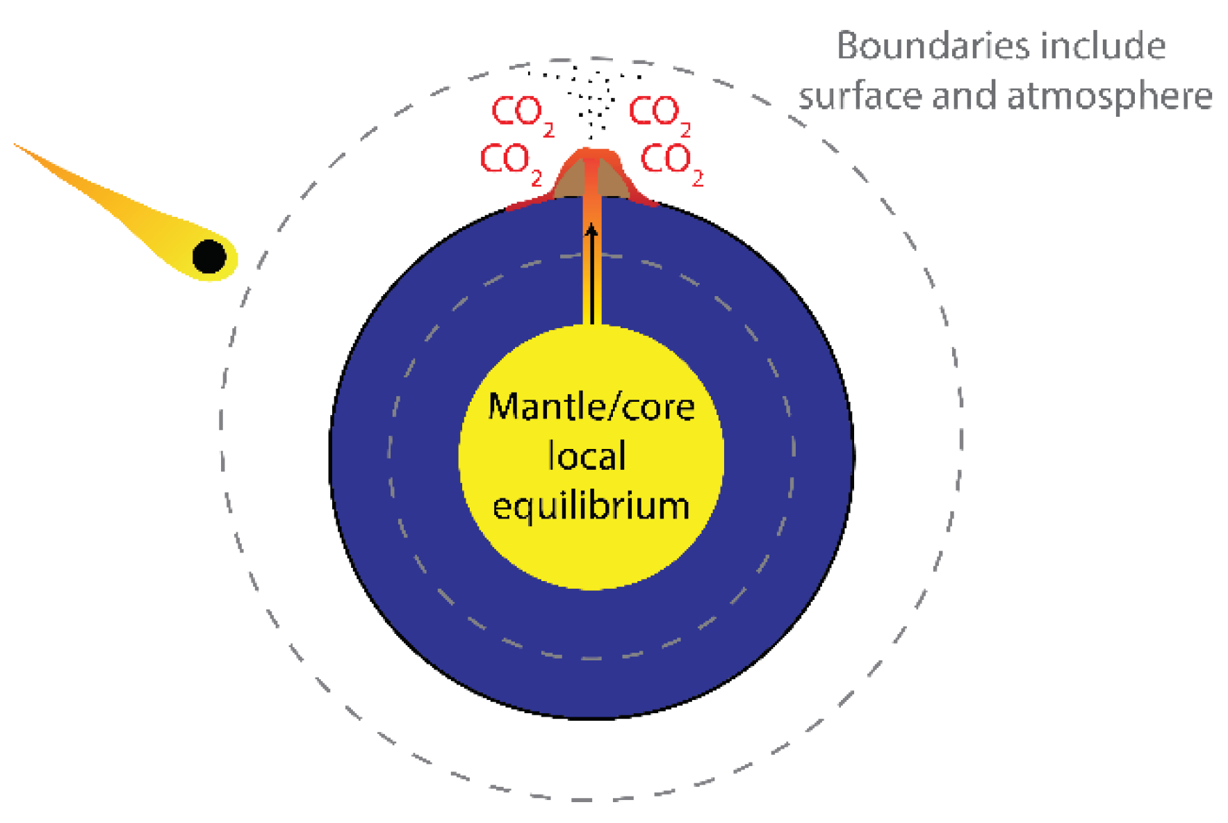
Viewing volcanic impulse inputs, which can also affect albedo and greenhouse gas concentrations, as external to the surface and atmosphere requires redrawing of the boundaries of Figure 1. In Figure 1, the boundary was drawn around the entire earth, which would include the mantel and core that are the source of volcanic activity. The boundary can be redrawn to include only the atmosphere and surface (Figure 8). The redrawing of the boundary in this way does not affect the energy and entropy balances described above, since the radiation inputs and outputs are so much larger in magnitude than the volcanic activity when averaged over time. However, this redrawing of the boundary makes the volcanic impulses external to Gaia, and therefore those inputs are boundary interactions and not subject to the governing principle. They are externalities, and like celestial body impacts, Gaia is expected to damp out the volcanic impulse boundary interactions, which is notion that is consistent with prehistorical climate evidence.[37] The core and mantel being governed by local equilibrium seems like a reasonable assumption. To our current knowledge, there is no external energy source to supply the core, and the energy flux from the core directed outwards is small with respect to the radiation exchanges with space at the surface.
5. Conclusions
In this work, satellite data from the MODIS and CERES instruments were analyzed to determine how the sunlight absorbed by the earth and entropy generated by the earth have changed over the time period from 2002 to 2023. It was found that the absorbed sunlight has increased significantly over the last 20 years, consistent with recent reports that the earth albedo has decreased over the same period. The entropy generation rate by the earth appears to have displayed significant stochastic fluctuations over the last 20 years but has oscillated about its mean value. Uncertainties in the entropy exchanges caused by the temperatures used in the calculations could be reduced if new satellite instruments became available that would directly measure the spectral irradiance of shortwave and longwave outputs with sufficient resolution to calculate the entropy flux as a function of position without the need for specifying a temperature. The results presented herein support the MPP but do not rule out the MEP. Since evolution towards decreasing albedo can be expected from both principles, societal efforts to harvest sunlight in the desert for e.g. electricity production are expected to be successful; but efforts to seed aerosols in the atmosphere to reflect more sunlight are expected to be unsuccessful. Externalities, that is perturbations originating from outside the system comprised of earth surface and atmosphere, are expected to damp out over geological time periods as global evolution points probabilistically towards the extremum expected by the MPP or MEP. Given that human society has become impactful enough to change the global environment, the results presented herein imply there may be an intimate connection between the evolution of human society and progress of the system comprised of the earth surface and atmosphere towards an extremum. That connection may prove useful for forecasting in the social sciences.
Author Contributions
This work was conceived of and created solely by the author. .
Funding
This work was not externally funded.
Data Availability Statement
The dataset used for this work is rather large, approximately 3 GB. Specific requests for data should be sent to the author. The CERES and MODIS data products can be downloaded from NASA via the internet. .
Acknowledgments
The McKelvey School of Engineering at Washington University is acknowledged for support while the author was on sabbatical, during which this work was conceived. .
Conflicts of Interest
The author declares no conflicts of interest.
References
- Waters, C.N.; Zalasiewicz, J.; Summerhayes, C.; Barnosky, A.D.; Poirier, C.; Gałuszka, A.; Cearreta, A.; Edgeworth, M.; Ellis, E.C.; Ellis, M.; et al. The Anthropocene is functionally and stratigraphically distinct from the Holocene. Science 2016, 351, aad2622. [Google Scholar] [CrossRef] [PubMed]
- Kasting, J.F. What caused the rise of atmospheric O2? Chemical Geology 2013, 362, 13–25. [Google Scholar] [CrossRef]
- Lovelock, J.E.; Margulis, L. Atmospheric homeostasis by and for the biosphere: the gaia hypothesis. Tellus 1974, 26, 2–10. [Google Scholar] [CrossRef]
- Wu, H.; Murray, N.; Menou, K.; Lee, C.; Leconte, J. Why the day is 24 hours long: The history of Earth’s atmospheric thermal tide, composition, and mean temperature. Sci. Adv. 2023, 9, eadd2499. [Google Scholar] [CrossRef]
- Archer, D.; Eby, M.; Brovkin, V.; Ridgwell, A.; Cao, L.; Mikolajewicz, U.; Caldeira, K.; Matsumoto, K.; Munhoven, G.; Montenegro, A.; et al. Atmospheric Lifetime of Fossil Fuel Carbon Dioxide. Annual Review of Earth and Planetary Sciences 2009, 37, 117–134. [Google Scholar] [CrossRef]
- Hall, C.A.S.; McWhirter, T. Maximum power in evolution, ecology and economics. Phil. Trans. R. Soc. A 2023, 381, 20220290. [Google Scholar] [CrossRef]
- Kleidon, A. A basic introduction to the thermodynamics of the Earth system far from equilibrium and maximum entropy production. Phil. Trans. R. Soc. B 2010, 365, 1303–1315. [Google Scholar] [CrossRef]
- Kleidon, A. Beyond Gaia: Thermodynamics of Life and Earth System Functioning. Climatic Change 2004, 66, 271–319. [Google Scholar] [CrossRef]
- Kleidon, A. How does the Earth system generate and maintain thermodynamic disequilibrium and what does it imply for the future of the planet? Phil. Trans. R. Soc. A 2012, 370, 1012–1040. [Google Scholar] [CrossRef]
- Kleidon, A.; Malhi, Y.; Cox, P.M. Maximum entropy production in environmental and ecological systems. Phil. Trans. R. Soc. B 2010, 365, 1297–1302. [Google Scholar] [CrossRef]
- Kleidon, A.; Lorenz, R. Non-equilibrium thermodynamics and the production of entropy life, earth, and beyond. In Understanding complex systems; Springer: Berlin; New York, 2005; pp xix, 260 p.
- Kleidon, A. Non-equilibrium thermodynamics, maximum entropy production and Earth-system evolution. Phil. Trans. R. Soc. A 2010, 368, 181–196. [Google Scholar] [CrossRef]
- Swenson, R. A grand unified theory for the unification of physics, life, information and cognition (mind). Phil. Trans. R. Soc. A 2023, 381, 20220277. [Google Scholar] [CrossRef]
- Dewar, R. Information theory explanation of the fluctuation theorem, maximum entropy production and self-organized criticality in non-equilibrium stationary states. J. Phys. A 2003, 36, 631–641. [Google Scholar] [CrossRef]
- Martyushev, L.M. Maximum entropy production principle: history and current status. Phys-Usp+ 2021, 64, 558–583. [Google Scholar] [CrossRef]
- Paltridge, G.W. Stumbling into the MEP Racket: An Historical Perspective. In Non-equilibrium Thermodynamics and the Production of Entropy: Life, Earth, and Beyond, Kleidon, A.; Lorenz, R.D., Eds. Springer: Berlin, Heidelberg, 2005. [Google Scholar]
- Gardner, C.S.; Liu, A.Z.; Marsh, D.R.; Feng, W.; Plane, J.M.C. Inferring the global cosmic dust influx to the Earth's atmosphere from lidar observations of the vertical flux of mesospheric Na. Journal of Geophysical Research: Space Physics 2014, 119, 7870–7879. [Google Scholar] [CrossRef]
- Schulz, L.; Glassmeier, K.-H. On the anthropogenic and natural injection of matter into Earth’s atmosphere. Advances in Space Research 2021, 67, 1002–1025. [Google Scholar] [CrossRef]
- Goode, P.R.; Pallé, E.; Shoumko, A.; Shoumko, S.; Montañes-Rodriguez, P.; Koonin, S.E. Earth's Albedo 1998–2017 as Measured From Earthshine. Geophysical Research Letters 2021, 48, e2021GL094888. [Google Scholar] [CrossRef]
- Loeb, N.G.; Priestley, K.J.; Kratz, D.P.; Geier, E.B.; Green, R.N.; Wielicki, B.A.; Hinton, P.O. R.; Nolan, S.K. Determination of Unfiltered Radiances from the Clouds and the Earth’s Radiant Energy System Instrument. Journal of Applied Meteorology 2001, 40, 822–835. [Google Scholar] [CrossRef]
- Loeb, N.G.; Doelling, D.R.; Wang, H.; Su, W.; Nguyen, C.; Corbett, J.G.; Liang, L.; Mitrescu, C.; Rose, F.G.; Kato, S. Clouds and the Earth’s Radiant Energy System (CERES) Energy Balanced and Filled (EBAF) Top-of-Atmosphere (TOA) Edition-4.0 Data Product. Journal of Climate 2018, 31, 895–918. [Google Scholar] [CrossRef]
- Wan, Z.; Zhang, Y.; Zhang, Q.; Li, Z.-l. Validation of the land-surface temperature products retrieved from Terra Moderate Resolution Imaging Spectroradiometer data. Remote Sensing of Environment 2002, 83, 163–180. [Google Scholar] [CrossRef]
- Walton, C.C.; Pichel, W.G.; Sapper, J.F.; May, D.A. The development and operational application of nonlinear algorithms for the measurement of sea surface temperatures with the NOAA polar-orbiting environmental satellites. Journal of Geophysical Research: Oceans 1998, 103, 27999–28012. [Google Scholar] [CrossRef]
- Landau, L. On the Thermodynamisc of Photoluminescence. Journal of Physics 1946, 10, 503–506. [Google Scholar]
- Rosen, P. Entropy of Radiation. Phys. Rev. 1954, 96, 555–555. [Google Scholar] [CrossRef]
- Ore, A. Entropy of Radiation. Phys. Rev. 1955, 98, 887–888. [Google Scholar] [CrossRef]
- Minnis, P.; Sun-Mack, S.; Young, D.F.; Heck, P.W.; Garber, D.P.; Chen, Y.; Spangenberg, D.A.; Arduini, R.F.; Trepte, Q.Z.; Smith, W.L.; et al. CERES Edition-2 Cloud Property Retrievals Using TRMM VIRS and Terra and Aqua MODIS Data—Part I: Algorithms. IEEE Transactions on Geoscience and Remote Sensing 2011, 49, 4374–4400. [Google Scholar] [CrossRef]
- Volk, T. The properties of organisms are not tunable parameters selected because they create maximum entropy production on the biosphere scale: A by-product framework in response to Kleidon. Climatic Change 2007, 85, 251–258. [Google Scholar] [CrossRef]
- Tester, J.W.; Modell, M. Thermodynamics and its Applications., 3rd ed.; Prentice Hall PTR: Upper Saddle River, N.J, 1997. [Google Scholar]
- Kondepudi, D.; Prigogine, I. Modern thermodynamics from heat engines to dissipative structures., 2nd ed.; John Wiley & Sons Inc.: Chichester, West Sussex, 2015. [Google Scholar]
- Chen, X.; Thimsen, E. Stationary states of hydrogen-producing reactions in nonequilibrium plasma. AICHE J. 2022, 69, e17952. [Google Scholar] [CrossRef]
- Thimsen, E. Entropy production and chemical reactions in nonequilibrium plasma. AICHE J. 2021, 67, e17291. [Google Scholar] [CrossRef]
- Uner, N.B.; Thimsen, E. Superlocal chemical reaction equilibrium in low temperature plasma. AICHE J. 2020, 66, e16948. [Google Scholar] [CrossRef]
- Lawrence, M.G.; Schäfer, S.; Muri, H.; Scott, V.; Oschlies, A.; Vaughan, N.E.; Boucher, O.; Schmidt, H.; Haywood, J.; Scheffran, J. Evaluating climate geoengineering proposals in the context of the Paris Agreement temperature goals. Nat. Comm. 2018, 9, 3734. [Google Scholar] [CrossRef] [PubMed]
- Valero, F.P. J.; Pilewskie, P. Latitudinal survey of spectral optical depths of the Pinatubo volcanic cloud-derived particle sizes, columnar mass loadings, and effects on planetary albedo. Geophysical Research Letters 1992, 19, 163–166. [Google Scholar] [CrossRef]
- Minnis, P.; Harrison, E.F.; Stowe, L.L.; Gibson, G.G.; Denn, F.M.; Doelling, D.R.; Smith, W.L. Radiative Climate Forcing by the Mount Pinatubo Eruption. Science 1993, 259, 1411–1415. [Google Scholar] [CrossRef] [PubMed]
- Scotese, C.R.; Song, H.; Mills, B.J. W.; van der Meer, D.G. Phanerozoic paleotemperatures: The earth’s changing climate during the last 540 million years. Earth-Science Reviews 2021, 215, 103503. [Google Scholar] [CrossRef]
- Vellekoop, J.; Sluijs, A.; Smit, J.; Schouten, S.; Weijers, J.W.H.; Sinninghe Damsté, J.S.; Brinkhuis, H. Rapid short-term cooling following the Chicxulub impact at the Cretaceous–Paleogene boundary. PNAS 2014, 111, 7537–7541. [Google Scholar] [CrossRef]
Figure 1.
System definition for thermodynamic analysis. The boundary is the top of atmosphere.
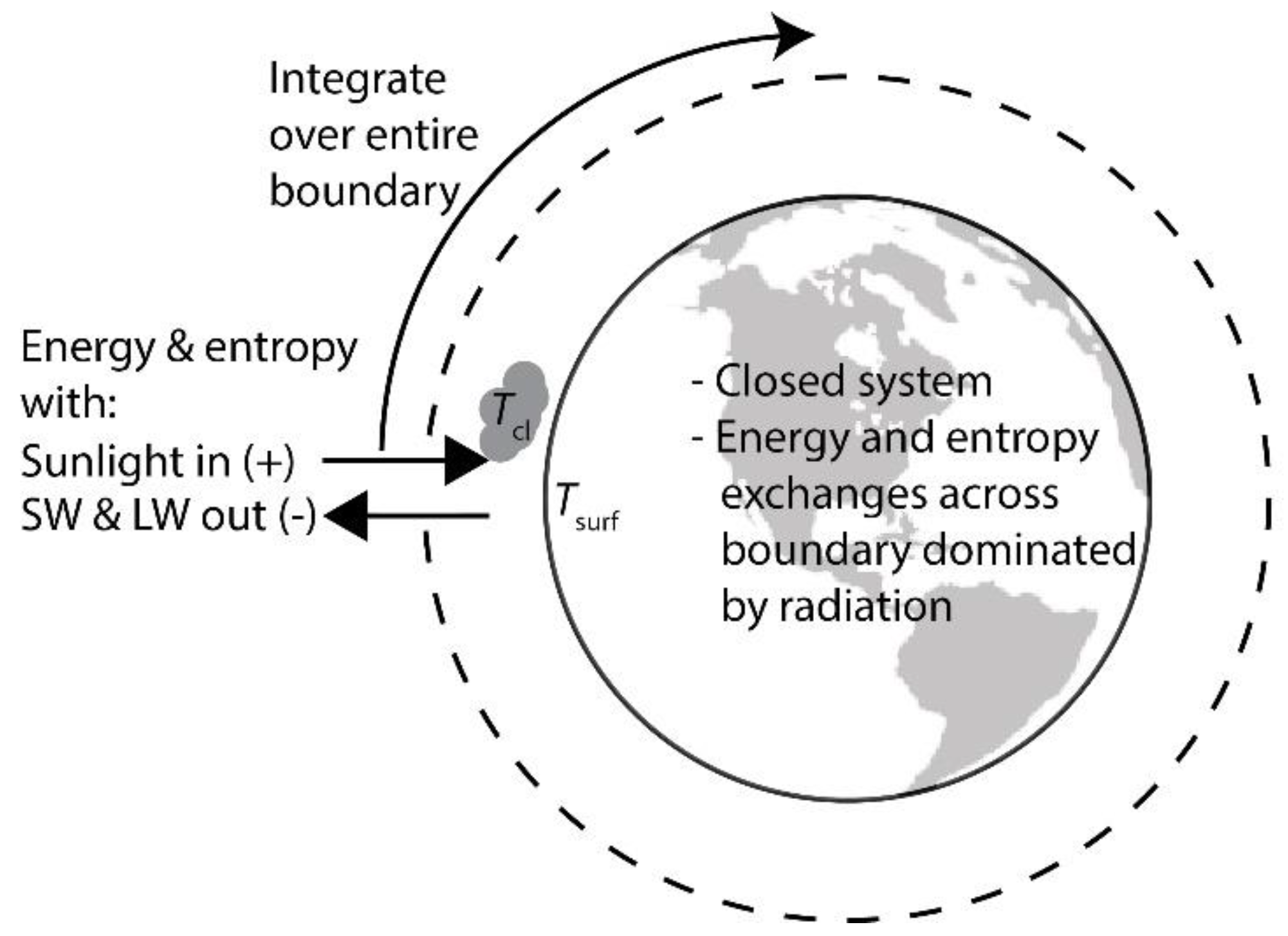
Figure 2.
Example snapshot of temperature data averaged over the month of May 2005. (a) Cloud area fraction, (b) cloud temperature, (c) land surface temperature during the day, (d) land surface temperature during the night, (e) surface temperature of the sea, and (f) composite surface temperature of land and sea using a time-average of day and night land temperatures.
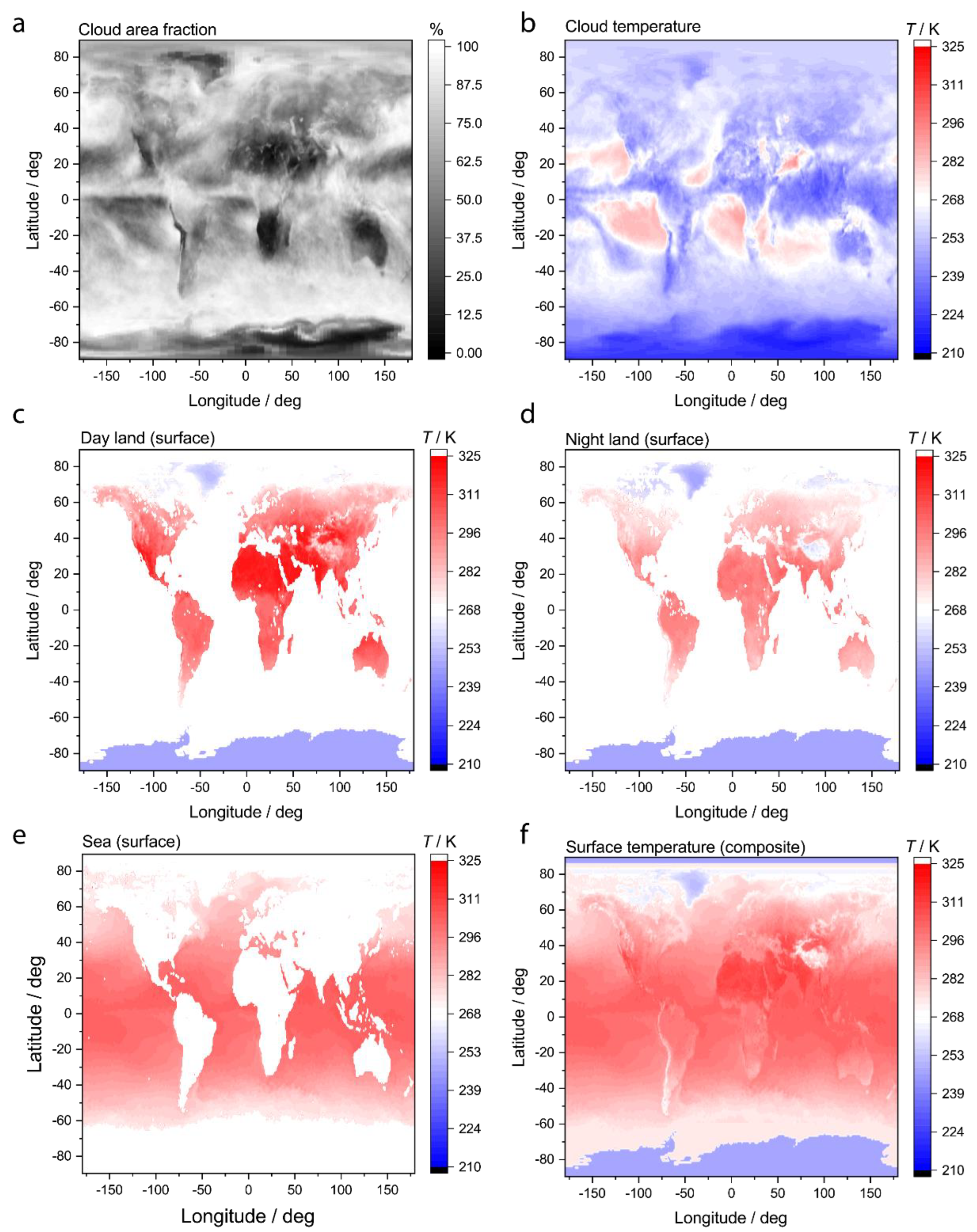
Figure 3.
Net exchanges of radiation with space. (a) Example map of the net radiation exchange as a function of position for the month of May 2005. (b) Globally integrated radiation exchanges as a function of time.
Figure 3.
Net exchanges of radiation with space. (a) Example map of the net radiation exchange as a function of position for the month of May 2005. (b) Globally integrated radiation exchanges as a function of time.
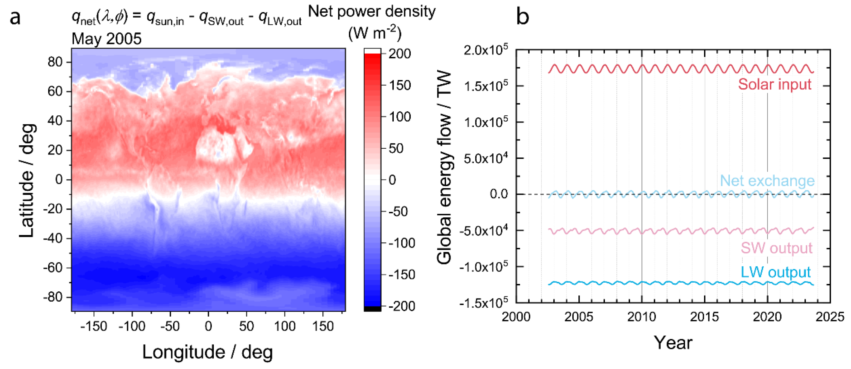
Figure 4.
Absorbed sunlight. (a) Globally integrated solar input minus SW output. (b) Globally integrated solar input minus SW output relative to 2003. The grey line is the raw data in (b) and the orange line is a moving average with a window of 12 months.
Figure 4.
Absorbed sunlight. (a) Globally integrated solar input minus SW output. (b) Globally integrated solar input minus SW output relative to 2003. The grey line is the raw data in (b) and the orange line is a moving average with a window of 12 months.
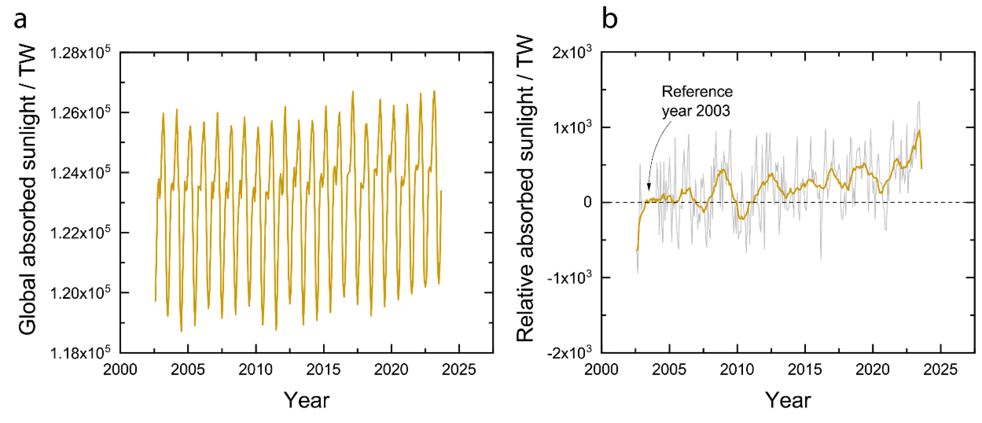
Figure 5.
Average surface and cloud temperatures. (a) Area-weighted average surface (red) and cloud (blue) temperatures. Area-weighted average (b) surface and (c) cloud temperatures relative to 2003. The colored lines in (b) and (c) are moving averages with a width of 12 months.
Figure 5.
Average surface and cloud temperatures. (a) Area-weighted average surface (red) and cloud (blue) temperatures. Area-weighted average (b) surface and (c) cloud temperatures relative to 2003. The colored lines in (b) and (c) are moving averages with a width of 12 months.
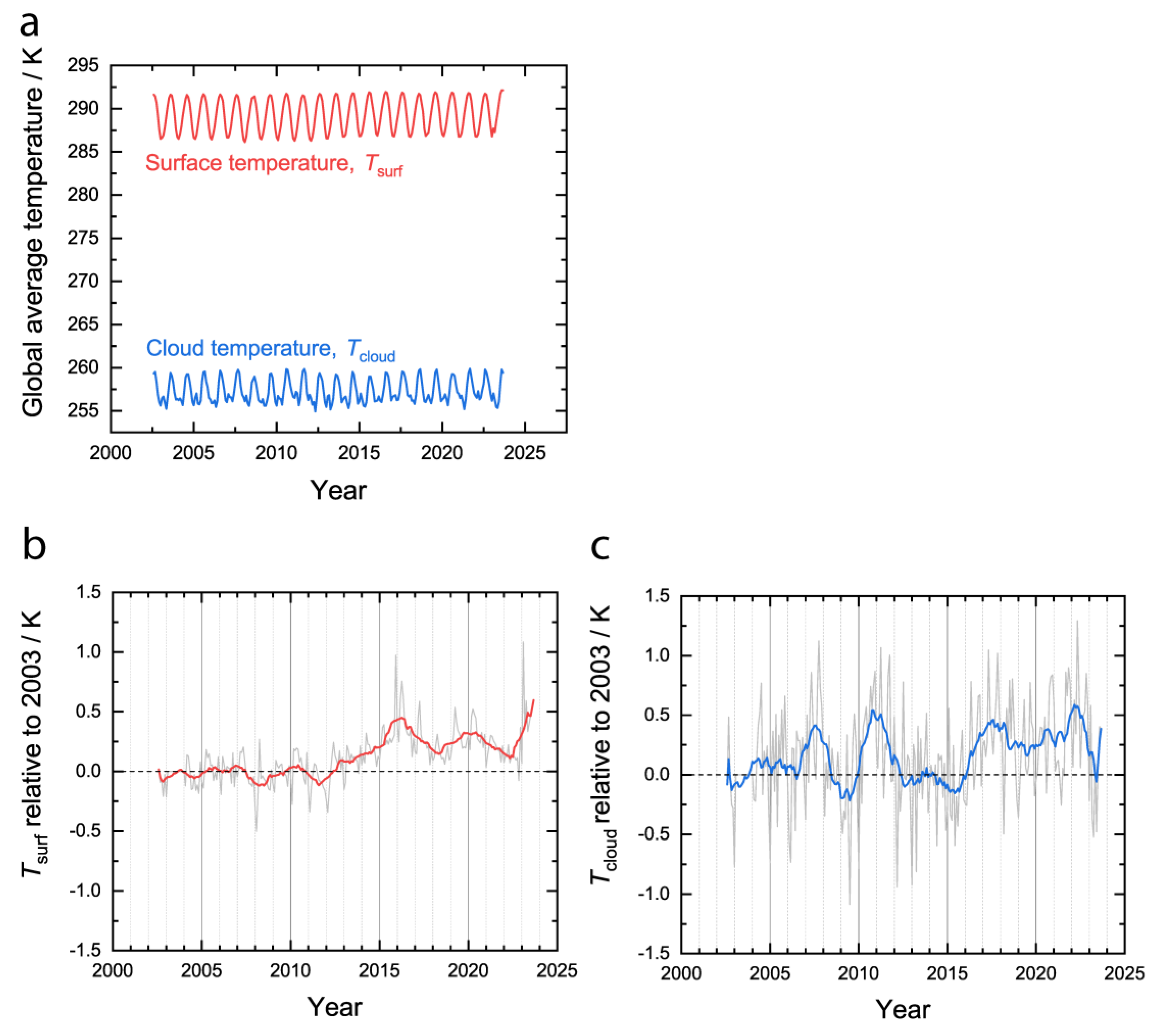
Figure 6.
Global distribution of radiation energy and entropy flux during the summer and winter. Net energy flux for (a) January 2005 and (c) July 2005. Net Entropy flux for (b) January 2005 and (d) July 2005.
Figure 6.
Global distribution of radiation energy and entropy flux during the summer and winter. Net energy flux for (a) January 2005 and (c) July 2005. Net Entropy flux for (b) January 2005 and (d) July 2005.
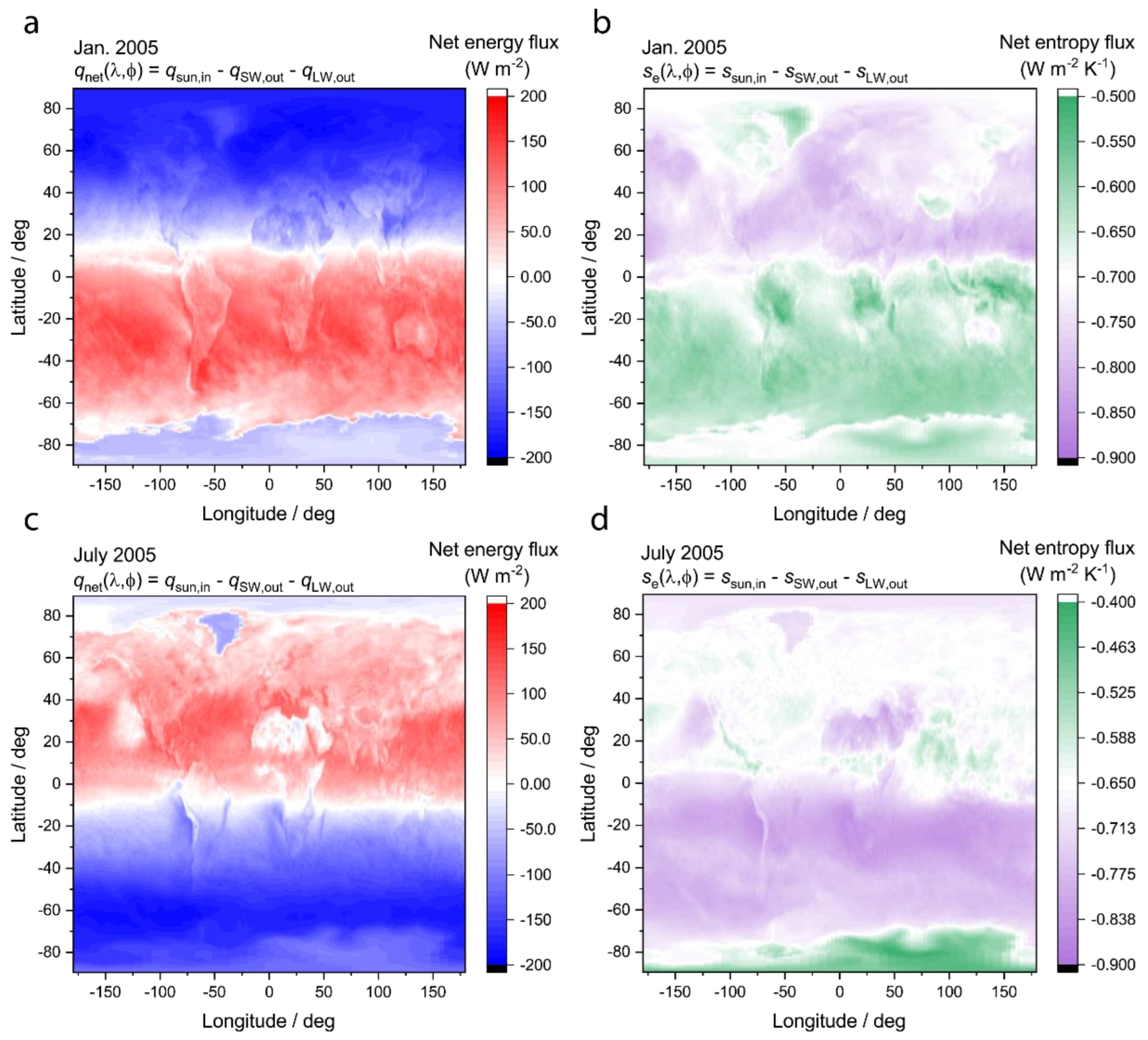
Figure 7.
Global absorbed sunlight and entropy production rate. (a) Global absorbed sunlight (orange) and entropy production rate (purple). Global entropy production rate (b) and absorbed sunlight (c) relative to the year 2003. The dark lines in (b) and (c) are moving averages with a 12 month window and the grey lines are the raw data.
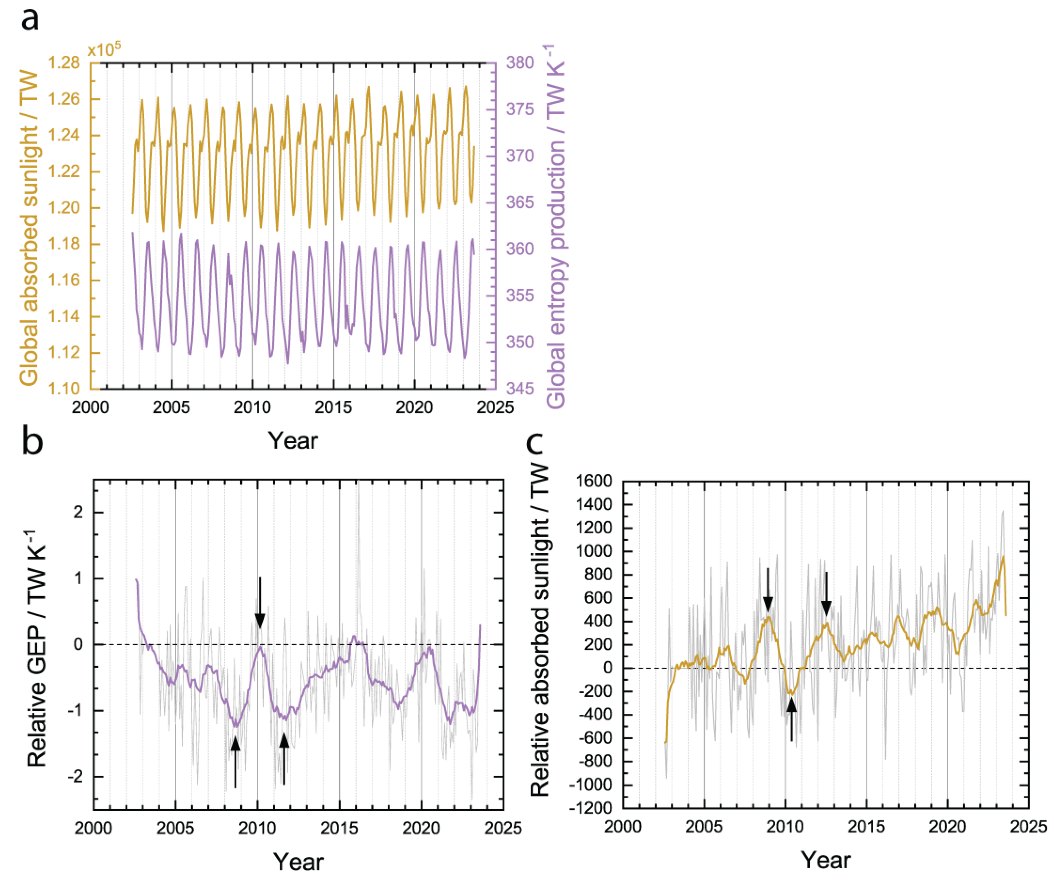
Figure 8.
Externalities and a revised definition of the system boundary. Externalities such as celestial body impacts and volcanic activity are considered as boundary interactions and are therefore not part of the system that is subject to MPP or MEP. Note: the revision of the system boundaries in this way does not change any of the empirical conclusions of this work (i.e. Figure 2, Figure 3, Figure 4, Figure 5, Figure 6 and Figure 7).
Disclaimer/Publisher’s Note: The statements, opinions and data contained in all publications are solely those of the individual author(s) and contributor(s) and not of MDPI and/or the editor(s). MDPI and/or the editor(s) disclaim responsibility for any injury to people or property resulting from any ideas, methods, instructions or products referred to in the content. |
© 2024 by the authors. Licensee MDPI, Basel, Switzerland. This article is an open access article distributed under the terms and conditions of the Creative Commons Attribution (CC BY) license (http://creativecommons.org/licenses/by/4.0/).
Copyright: This open access article is published under a Creative Commons CC BY 4.0 license, which permit the free download, distribution, and reuse, provided that the author and preprint are cited in any reuse.


