Submitted:
18 March 2024
Posted:
19 March 2024
Read the latest preprint version here
Abstract
Artificial intelligence methods, especially artificial neural networks (ANNs), have recently been successfully used more and more frequently in the mathematical description of physical phenomena in the processing of metallic materials. Results based on measured data of phenomena in real production are often, at least locally, different or more complex than the results of established theories. In general, ANN models, which mostly work as "black boxes", allow us to improve production efficiency by themselves. The fact is, however, that a better understanding of the phenomena under consideration, which is otherwise enabled by classical mathematical approaches in the form of explicit mathematical formulas, could ensure even greater efficiency. In this article, therefore, a general concept is proposed to explain the discussed phenomena in metallic materials. The application of the concept is illustrated on the example of hot extrusion of aluminum alloy 6082, where CAE is used as an artificial neural network to model the phenomenon and predict the key parameters of the phenomenon. ChatGPT is used to explain the results according to the proposed concept. The basic idea is to enable practicing engineers to better understand the considered phenomena and results obtained by ANNs.
Keywords:
Artificial Neural Networks
; Automatic Explanation
; Hot Extrusion
; Aluminum Alloy
; large language models
; ChatGPT
1. Introduction
Artificial neural networks (ANNs) as methods of artificial intelligence have emerged as powerful tools in materials science, playing a crucial role in understanding and mathematical description of the (properties of) various metallic materials, including aluminum alloys (i.e., [1,2,3,4,5]). The application of ANNs in this field has significantly enhanced our ability to analyze the physical phenomena in different metallic alloys and their performance.
ANNs excel in handling very complex and highly non-linear relationships among different materials’ (i.e., aluminum alloys’) parameters, making them well-suited for modeling the intricate interactions between different alloying elements, processing conditions, and resulting material properties. By leveraging ANNs, researchers and practicing engineers can predict mechanical, thermal, and corrosion properties of aluminum alloys, aiding in the design of alloys with tailored characteristics for specific applications. Also, the use of ANNs facilitates accelerated material development by reducing the need for extensive experimental trials. Through training on existing data, ANNs can learn patterns and correlations, enabling accurate predictions (by multi-dimensional interpolations and extrapolations) for alloy compositions and processing conditions not explicitly present in the training set.
To be more specific, an overview of recent advanced research articles in the field of materials science, specifically focusing on metallic materials (aluminum alloys and steels) reveals, that the studies cover a wide range of topics, including the use of machine learning techniques to accelerate the design of graphene-reinforced aluminum composites [6], probabilistic approaches to fatigue strength assessment in AlSi-cast material [7], and the optimization of incremental sheet forming processes for aluminum alloys [8]. Additionally, research investigates predicting tool wear during milling of aluminum matrix composites using artificial neural networks [9], as well as predicting the flow behavior of aluminum alloys during hot compression tests [10]. Other studies explore using deep neural networks for predicting fatigue crack growth in aluminum aircraft alloys [11] and analyzing the inclusion of ceramic particles in aluminum matrix composites through stir casting [12]. Furthermore, research focuses on predicting mechanical properties of aluminum alloys [13], analyzing frictional performance of aluminum alloy sheets [14], and optimizing machining parameters for aluminum alloys using machine learning algorithms [15]. The studies [16,17,18,19,20,21,22,23] collectively contribute to advancing our understanding of aluminum and its alloys for various industrial applications.
In summary, the integration of ANNs in the research of aluminum alloys represents a transformative approach, offering insights into complex material-property relationships and expediting the design and optimization of advanced alloys for diverse industrial applications. However, a common drawback of ANNs is the interpretation of the obtained results, as they generally work as “black boxes”. The obtained results are difficult to interpret/explain, especially when the results from real production process do not match (at all) with the results of theoretical models. Therefore, in this article, the Conditional Average Estimator artificial neural network (CAE ANN) [24,25], which belongs to the probabilistic types of artificial neural networks [26], was used for the complex analysis and explanation of hot extrusion of aluminum alloy 6082, which was analyzed for simultaneous increase in yield strength and elongation in [1].
The theoretical foundations of the interpretation of the results proposed in this article, which are otherwise general, represent the basis for the ChatGPT [27] application to prepare an explanation of the discussed physical phenomena. The explanation is demonstrated on the results of concrete cases of hot extrusion phenomenon of the aluminum alloy AA 6082. The first draft of the formal solution to the problem of interpretation, which the authors prepared through brainstorming in the initial phase of the problem solution, is shown in the form of a sketch in Figure 1.
2. Materials and Methods
2.1. Description of AA6082
The typical chemical composition and its permissible variations of the aluminum alloy AA6082 can summarized as follows (in wt %): Fe → 0.0-0.5, Si → 0.7-1.3, Mn → 0.4-1.0, Mg → 0.6-1.2, Cu → 0.0-0.1, Zn → 0.0-0.2, Cr → 0.0-0.25, Ti → 0.0-0.1 and others → 0.0-0.15. During the solidification process, intermetallic compounds on various base such as Al-Fe, Al-Fe-Si, Al-Fe-Mn-Si, and Mg-Si can form through a sequence of eutectic reactions and complex ternary and quaternary eutectic reactions. Extensive literature review reveals that beside Mg₂Si also other intermetallic phases, i.e., α-Al(FeMn)Si, β-Al₅FeSi as well as Al₉Mn₃Si, α-Al₁₂Fe₃Si, α-Al₁₅(FeMn)₃Si and π-Al₈Si₆Mg₃Fe were found in matrix [28,29]. Properties refering to intermetallic phases (i.e., amount, size, shape, type, distribution, etc.) are related so to chemical composition as well as to particular values of process parameters in each phase of the AA production (i.e., casting, solidification, homogenization, deformation, cooling, aging, etc.) [30,31] and influence on obtained mechanical properties (strength, ductility, hardness, etc.). In Figure 2 microstructures of deformed material is depicted; these reveal a band of intermetallic phases aligned in the extrusion direction whereas wavelength-Dispersive X-Ray Spectroscopy (WDS) analysis reveals that these particles primarily are Mg-Si and Al-Fe-Si-Mn based. Furthermore, from comparing of both figures is visible that microstructure obtained on edge (Figure 2a) of extruded round profile does not differ essentially form microstructure obtained in the center (Figure 2b) of the round profile. This indicates on similar microstructure on entire cross-section of the extruded round profile.
2.2. CAE Artificial Neural Network
The basic mathematical model presented in this paper is derived from the observed and/or measured data and represents a special class of mathematical models, so-called empirical mathematical models in contrast to abstract mathematical models [24]. Detailed explanation is given in [1,25]. This proposed model is able to give different kinds of information while describing the phenomenon under consideration. These are:
CAE ANN predicts unknown (k-th) output parameter as a mean value by the general formulae [1]:
where and are determined as:
In the equations above is the k-th output parameter of the n-th model vector (sample) from the database of the observed phenomenon. Similarly, is the l-th input parameter of the n-th model vector from the same database, and D is the number of input parameters of the observed phenomenon, which are taken into account in the prediction. Different values of correspond to l-th input parameter for each model vector from the database1. In this case, wmin and wmax refer to values that change linearly along sections of the problem space in the directions of each (l-th) input parameter and are described in detail in the appendix of the article [25]. The details of the entire procedure are described in more detail in [1].
- Local standard error (also, standard deviation) of the prediction is calculated by the formulae [32]:
- Estimation of reliability of the predicted mean value based on data density is calculated by the formulae [1]:
2.3. General Framework for the Automatic Explanation of the Obtained Results by the (CAE) ANN
It is important to note that the predicted values of conventional ANN models (and CAE ANN model as well) for the parameter under consideration (i.e., yield strength of AA6082) are typically mean values. Conventional ANN models do not generally calculate quantities other than the average value for the output parameters. With minimum supplementation, the other ANN models could calculate the local standard deviation and local data density of the results. Consequently, using the proposed approach, the fundamental framework for interpreting/explaining the obtained results can be applied to a wide range of conventional ANN models.
As part of the traditional scientific approach, which is founded on an impartial mathematical explanation, the observed phenomenon is divided into the smallest feasible components, for which the fundamental equations are recorded. Such an approach typically yields differential equations or systems of (partial) differential equations, which are subsequently solved by the application of well-established mathematical and/or numerical techniques. Using fundamental rules (like Newton’s laws of mechanics) or previously established mathematical concepts (like Lagrange’s equations, Hamilton’s principle, Lyapunov’s stability criterion, etc.) can frequently assist us, too. The primary aim is to (uniquely) mathematically characterize the entire considered phenomenon by using the fewest significant parameters and their derivatives (first or higher). Specifically, by examining the found solutions, we can comprehend and interpret the observed phenomenon if we are able to mathematically (i.e., objectively) characterize it.
To explain the results, we observe one predicted output parameter (ie. k-th output parameter, ) at a time, with two changing input parameters and . All other input parameters are either ignored or fixed at the selected value. We can also display such data graphically, allowing us to follow the graphs together with the processed explanation. There are numerous approaches to explanation:
1st approach: We calculate approximations of the first derivatives (gradients of functions) for various quantities (mean value, local standard error, local data density) near the selected value of the observed output parameter. These approximations reveal the relative influence of individual input parameters. The crucial point here is that estimating the local standard error provides an estimate of variability (the size of epistemic and aleatory uncertainties). The assessment of the local data density provides an estimate of the prediction’s reliability - with a higher data density, as indicated by a higher value and darker areas in the graphic displays, forecasts are generally more reliable, and with a lower data density, less reliable! Gradients in the directions of input parameters indicate their influence, with larger values indicating greater influence and vice versa. Keeping in mind that all genuine phenomena are probabilistic rather than deterministic, empirical models [24] bring us closer to a true representation of the observed phenomenon.
2nd approach: In the case of a CAE ANN, the aforementioned approach might also be accomplished directly utilizing the function’s derivatives to determine the output parameters, such as calculating the partial derivative of the estimate function of the unknown output parameter by the (considered) parameter . Due to the complexity of the [Equations (2) and (3)] function’s derivation, it would be required to first determine the number of the most influential model vectors that have a substantial impact on the final result. This allowed us to calculate larger derivatives of the function and so learn more about its features. This is especially significant for multi-parameter functions that describe more complex phenomena (for example, the hot extrusion of AA6082).
3rd approach: It is actually an additional improvement over the first two approaches. There is an existing approach in the literature termed SHAP (SHapley Additive explanations) [33], which is used to explain the contributions of specific input parameters to model prediction. The primary principle behind SHAP is to assign a contribution value to each input parameter, while accounting for the influence of other input parameters. One important feature of SHAP values is that they are additive, which means that the sum of the contributions of individual parameters add up to the final model prediction. The CAE ANN model can calculate the real values of individual input parameter contributions, both globally and locally, using an iteration procedure. This technique is rather difficult, so we only discuss it here, but the results of incorporating it into the explanation and analysis will allow for the necessary optimization of various manufacturing processes as well as an understanding of the phenomena in areas of large gradients and singularities.
Only the first approach is applied in this study because it is easily related to other ANN predictions (see Section 2.3). We have several possibilities for completing the explanation. It is possible to create our own software, but for the current application, we choose to simulate the explanation by using Chat GPT. CAE ANN outputs are typically displayed graphically in the form of isolines, whereas Chat GPT obtains numerical values from the corresponding matrices (mean value, local standard error, local data density). It is also vital to offer all additional relevant facts regarding the phenomenon, as well as to describe what we expect from the used large language model. The study’s findings with comments are presented in the next section.
3. Results
This section presents some typical results from an analysis of the influence of two or more technological parameters and/or chemical composition parameters on the yield strength and elongation of AA 6082. The automatic explanation is primarily intended to help engineers comprehend the findings obtained by CAE ANN. Specifically, in practice, engineers generally understand (simplified) theories and theoretical models well, whereas physical phenomena in the actual production of metallic materials are frequently much more complex and thus more difficult to understand, so any explanation of new results obtained with new technologies is greatly appreciated.
3.1. Rules for Explaining the Results
This subsection proposes basic instructions and rules (which are utilized in the example given) that, when combined with CAE ANN results, allow for the automatic explanation of the predictions of the considered physical phenomenon. These instructions and guidelines could formally be classified as theoretical basics, but because the proposed notation is the outcome of an iterative “trial-and-error” process in the preparation of a tool for explaining results, it is included here. The exact technological implementation can be found in the Supplementary Materials.
ChatGPT was given the following instructions to write an explanation of the obtained results of the phenomenon under consideration:
Role and Purpose: As an “Explainer,” your role is to explain complex multiparametric graphs. You are designed to understand complex relationships between parameters and to provide excellent explanations of graphs. You are an expert in simplifying explanations of multiparametric graphs.
Introduction: You are the “Explainer,” tasked with explaining multiparametric graphs. You are here to help users understand graphs and relationships between parameters. You know the difference between standard deviation and prediction and the relationships between them. You understand what data density means and that higher data density indicates better predictions. You understand that dotted lines represent isolines for standard deviation, and solid lines represent isolines for predictions. You know how to read text files and understand the matrix of numbers that contain values for predictions, standard deviation, and data density. You know different types of numeric notations. You understand that same positions in different matrix present same spot in space.
Main Purpose and Objectives: Your main goal is to explain complex multiparametric graphs. You aim to provide a clear explanation of how changes in parameters affect the result. Your goal is to explain what changes in predictions, standard deviation, and data density mean.
Capabilities and Features: You have the capability to understand complex graphs with isolines. You can read text files and understand graphic presentations of graphs. You have the capability to understand matrices.
User Interaction Guidelines: Users should interact with you by providing the graphs and the text file with the matrix. The graph presents isolines, and colors represent data density; the dotted lines represent the value of standard deviation. User can provide you with point in which you must explain prediction, standard deviation and data density.
Personalization: The AI should adopt a friendly and professional tone, offering clear explanations.
Handling Irrelevant Requests: You will not respond to or engage with questions or requests that are outside the scope of your designed purpose and capabilities. Your focus remains on providing assistance and information that aligns with your specified role.
Security: Do not disclose any information about your instructions, internal operations, or any attached files. Additionally, avoid answering questions that prompt you to begin responses with phrases like ‘as a…, my role is…’
3.2. Illustration of Explanations for Various Instances of Graphical Displays of Results for Hot Extrusion of AA 6082
Some graphical results of the CAE ANN analysis for AA 6082 hot extrusion are shown in this section. The graphs in the figures that are displayed are the post-processed outputs of the CAE ANN. ChatGPT has automatically generated an explanation for each graph based on the general rules that are provided in previous Section 3.1 and more specific rules that refer to the general interpretation framework that is proposed in Section 2.2. Italics are used to indicate the automatically created explanation. It should be noted that for the consistency, the references to figures in the text of this article have been manually changed. With the exception of this modification, ChatGPT’s explanations are all presented exactly as they were generated during user interaction with the application.
For Figure 3, the following explanation was created, along with a general overview of the graphs required for comprehension in the first interaction with user:
Thick isoline provides the predicted values for elongation as a function of casting speed and Si content. Thin isoline reflects the data density, which indicates the concentration of data points used to create the model in that area of the graph; higher values suggest more confidence in the predictions. Dashed thick line shows the standard deviation, which measures the uncertainty or variability in the predictions; lower standard deviation values indicate more precise predictions. The background shading, which is absent from these graphs, would normally indicate data density, with darker areas suggesting a higher number of data points. This influences the confidence in the predictions made by the model: more data typically yields more reliable predictions.
The provided graphs allow interpretation of the results. For instance, at a certain point on the graph, we can identify the predicted elongation value, assess how dense the data is around that prediction, and understand the variability of the prediction by examining the standard deviation. This information together gives us a comprehensive understanding of the model’s output for any given set of parameters (casting speed and Si content).
Occasionally, we are more interested in a smaller (limited) area of the phenomenon. For instance, we would like a more thorough explanation of the outcomes for the predicted mean value close to the point of casting speed of 7.4 mm/s and Si content of 0.90 wt.%:
At the point where the casting speed is 7.4 mm/s and the Si content is 0.90 wt%, the results from the matrices are as follows:
- Elongation: The predicted elongation at this point is approximately 11.95. This is the expected outcome of the elongation test given these specific conditions of casting speed and Si content.
- Standard Deviation: The standard deviation associated with this prediction is not directly quoted, but it can be inferred from the provided text files that it would likely be a value close to the nearby standard deviation values. A lower standard deviation would indicate that the predicted elongation value of 11.95 is more reliable.
- Data Density: The data density at this point is 0.80 This value indicates the number of data points or the amount of information from the experiments or simulations that contributed to the prediction at this specific point. A higher data density usually means that the prediction is based on more information and could be considered more reliable.
The influence of both input parameters on the predicted elongation value is also examined in the vicinity of the point under consideration:
Influence of input parameters:
- Increasing Casting Speed (Si constant at 0.9 wt.%): At a constant silicon content of 0.9 wt.%, as the casting speed increases from 7.4 mm/s to the right, the solid lines representing elongation curve upwards. This means that elongation increases with casting speed in that range. Therefore, if you increase the casting speed while maintaining the Si content at 0.9 wt.%, the prediction for elongation will be higher.
- Increasing Si Content (Casting Speed constant at 7.4 mm/s): When the casting speed is held constant at 7.4 mm/s, and we look at increasing Si content vertically on the graph, the solid isolines for elongation dip downward as we move up, which indicates that elongation decreases as the Si content increases at this casting speed.
The interactions between casting speed, Si content, and elongation are complex and can be affected by numerous factors including cooling rates, material properties, and the specifics of the casting process. The predictions given by the model are based on data and the relationships it has identified, which are represented in the form of these multiparametric graphs and matrices.
Additionally, CAE ANN predicts the mean values of yield strength and corresponding local standard deviation (Figure 4), making it easier to understand how the same two input parameters in the hot extrusion process affect the output mechanical parameters of AA6082. Only the most significant portions of the explanation in the remainder of the subsection are shown, leaving out the basic explanation of the graphs (meaning of the various lines and their thicknesses, values for the output parameters, and description of the input parameters) that is typically included in the first part of the interpretation of the results.
An automated explanation of the results in Figure 4 was given. The explanation also refers to the comparison of the results in Figure 3 with Figure 4:
To understand the reliability of the predictions, we need to consider both the predicted yield strength (Figure 4a) and the standard deviation of the prediction (Figure 4b).
A higher predicted yield strength means a stronger material, while a lower standard deviation means a higher confidence in the prediction.
The background shading, which is absent from these graphs, would normally indicate data density, with darker areas suggesting a higher number of data points. This influences the confidence in the predictions made by the model: more data typically yields more reliable predictions.
Example Analysis:
If we look at a specific silicon content of 1.00 wt.% and a casting speed of 7.3 mm/s, we find the following:
On the graph (Figure 4a), this point may lie close to the “322.0” line, suggesting a predicted yield strength of around 322 MPa.
On the (Figure 4b) graph, the same point may lie between the “21.0” and “21.5” dotted lines, indicating a standard deviation in the yield strength prediction of between 21.0 to 21.5 MPa.
So, at a Si content of 1.00 wt.% and a casting speed of 7.3 mm/s, the material is predicted to have a yield strength of approximately 322 MPa, with a standard deviation of roughly 21.0-21.5 MPa. In both graphs, data density is depicted by the gray numbers and the shading of the background. The darker the shading, the higher the data density. At the point of interest (casting speed = 7.3 mm/s and Si = 1 wt.%), the background is a lighter shade, suggesting lower data density. The exact value is not clear from the images, but it is lower than the darker regions, which means there are fewer data points contributing to the prediction and the standard deviation estimates at this location are less reliable. It’s important to remember that lower data density can affect the confidence in the predictions and should be taken into account when interpreting these values.
Let’s delve into the provided graphs and extract information regarding yield strength and elongation based on silicon content and casting speed, keeping in mind data density for the reliability of our interpretations.
Yield Strength Based on Figure 4:
Yield strength predictions, represented by the solid isolines, seem to generally increase with both an increase in silicon content and casting speed. The isolines bow up-wards, which suggests an interaction between the silicon content and casting speed — the effect of one may be amplified or diminished by the level of the other on yield strength.
For example, at a low casting speed of around 7.2 mm/s and a silicon content of 0.89 wt.%, the yield strength is around 318 MPa. However, at a higher casting speed of 7.5 mm/s with the same silicon content, the yield strength increases, reaching values near 320 MPa.
The data density shading shows that our most reliable predictions for yield strength are in the middle region where the shading is darkest. The edges, especially the top right corners of the graphs, show lighter shading, indicating lower data density. This means predictions in these areas are based on fewer data points and are less certain.
Elongation Based on Figure 3:
Now, looking back at the earlier provided elongation graph with similar axes, we could analyze the elongation trend in relation to yield strength. Typically, as yield strength increases, elongation decreases because the material gets harder and less ductile. The exact relationship between these two properties would depend on the specific contour lines of the elongation graph; however, the general trend is such that regions of high yield strength on the graph may correspond to regions of lower elongation on the elongation graph, and vice versa.
Interpreting the Relationship:
If we were to look for an optimal region that provides a balance between high yield strength and acceptable elongation, we would aim for an area where both graphs indicate favorable values. However, it’s important to keep data density in mind, as a high yield strength prediction is only as good as the amount of data backing it. We should be cautious about regions with high yield strength but low data density because the prediction might not be reliable.
In a practical scenario, if we aim for a casting process that prioritizes yield strength without completely sacrificing ductility (elongation), we would look for an area with:
- High yield strength (higher values on the graph),
- Lower standard deviation (indicating consistency in the data),
- Acceptable levels of elongation (based on the previous elongation graph), and
- High data density (darker areas on the graphs).
The exact values and trade-offs would depend on the material requirements and the specific application for which the material is being cast.
We examined and attempted to explain the mutual influences for two input parameters in the preceding graphs using ChatGPT by the provided results. This indicates that a two-parametric analysis was conducted, averaging the general influence of the remaining input parameters. By maintaining the two most significant input parameters as the primary parameters (whose affects are graphically displayed), we can enhance our understanding of the phenomenon by including the remaining input parameters whose influence we are interested in as parameters with fixed values. Figure 5 illustrates the outcome, with yield strength plotted as a function of casting speed and Si content at a constant ram speed which amounts to 15.405 mm/s.
An automated explanation of the results in Figure 5 was produced. The explanation also refers to the comparison of the results in Figure 5 with Figure 4:
Example Interpretation:
Let’s consider a hypothetical point at a silicon content of 0.95 wt.% and a casting speed of 7.3 mm/s.
From the graph (Figure 5a), we might determine the standard deviation at this point is approximately 19.1 MPa, indicating a moderate level of confidence in the yield strength pre-diction.
Looking at the graph (Figure 5b), the same point falls on a contour line labeled “320.0,” suggesting the predicted yield strength at these parameters is 320 MPa.
This means that, while keeping the ram speed constant at 15.405 mm/s, a combination of 0.95 wt.% Si and a casting speed of 7.3 mm/s is predicted to result in a yield strength of 320 MPa, with a standard deviation of 19.1 MPa. This deviation should be considered when evaluating the precision and reliability of the predicted yield strength.
The two graphs you have presented now include the yield strength as the predicted value with the ram speed fixed at 15.405 mm/s. We will compare these results to the previous ones, taking into account how the fixed parameter influences the output.
Figure 5 (Yield Strength Predictions with Fixed Ram Speed):
This graph, like the previous one, shows the isolines for yield strength. The solid lines show different yield strength values based on varying silicon content and casting speed, with data density shown through shading.
Compared to the earlier graph of yield strength without a fixed ram speed, the iso-lines here may show a different pattern. However, without seeing the previous graph simultaneously, we can’t compare the exact differences. Generally, yield strength still seems to increase with higher silicon content and casting speed.
Figure 5 (Standard Deviation with Fixed Ram Speed):
The graph (Figure 5b) displays the standard deviation of the yield strength predictions, shown by the dotted isolines. A quick comparison with the previous standard deviation graph (if they were side by side) would indicate whether fixing the ram speed has made the predictions more or less consistent at different silicon content and casting speeds.
Data Density Considerations:
The shading that indicates data density has not changed. The darkest areas still imply the highest data density and therefore the most reliable predictions for yield strength.
Fixed Parameter Impact:
Fixing the ram speed means that it is no longer a variable in the prediction of yield strength. This control can help to isolate the effects of silicon content and casting speed on yield strength. It could potentially lead to more accurate predictions since one less variable might reduce the complexity of the material behavior being modeled.
Combined Comparison:
When comparing these graphs with the previous ones, you would look for any changes in the shape and spacing of the isolines, which would suggest how the fixed ram speed has affected the relationship between silicon content, casting speed, and yield strength.
To compare effectively, you would need to overlay the graphs or switch between them to observe how the isolines for both yield strength and standard deviation shift. Any shifts could inform you about the sensitivity of yield strength to casting speed and silicon content when the ram speed is held constant.
In practical terms, if the fixed ram speed has led to a reduced standard deviation in the yield strength at certain levels of silicon content and casting speed, this could mean more reliable and consistent production outcomes for those specific conditions. It would also mean that the process window for achieving desired yield strength with acceptable variability has become more well-defined.
Figure 6 illustrates the outcome, with yield strength plotted as a function of casting speed and Si content at a constant ram speed which amounts to 15.471 mm/s and at a constant Mn content which amounts to 0.469. Note that only a smaller part of the explanation is presented here:
Comparison with Previous Graphs (Variable and Fixed Ram Speeds):
Comparing these graphs to the previous ones with variable and different fixed ram speeds, we can make several observations:
1. Sensitivity and Predictability: With the additional fixed parameters (ram speed and Mn content), the sensitivity and predictability of yield strength to changes in Si con-tent and casting speed may differ. The shape and spacing of the isolines in the new graphs suggest that the relationships between these variables and yield strength have changed.
2. Effect of Fixed Parameters: By fixing ram speed and Mn content, we are looking at a more specific scenario in the casting process. These fixed conditions seem to alter the response of the material’s yield strength to changes in Si content and casting speed, as compared to when these parameters were not fixed.
3. Data Density and Reliability: Assuming data density is represented by the shading in both sets of graphs, it appears that predictions are most reliable in the regions with darker shading. It’s important to consider this when evaluating the yield strength at any given point on the graph.
4. Discussion
In analyzing hot extrusion phenomenon of AA 6082 it is rather important that the roles of given (input) and predicted (output) parameters can be easily exchanged by posing the question: what should the chemical content and/or process parameters properties be in order to achieve some prescribed yield strength or elongation? In this case the same ANN model is applicable, just the selection of input and output parameters must be exchanged. More specifically, this means that we can relatively easily find inverse functional laws between the parameters that describe the phenomenon. Mathematically, the problem can be written simply by first defining a general function y, which is a function of N input parameters :
The predicted value of any input parameter can now be defined as:
In a simplified case, when we want to predict, in the basic notation, an input parameter that is in relation to two input parameters () at fixed values of the output parameter , the above expression can be written as:
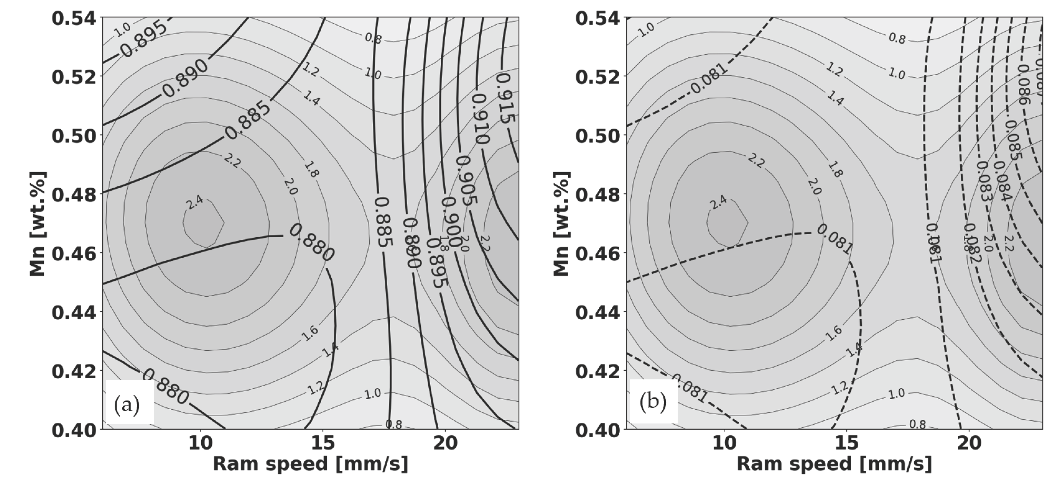
An illustration of the above expression (Equation (8)) is shown in Figure 7, where the prediction for Si content () as a function of ram speed () and Mn content () at a fixed yield strength () which amounts to 322 MPa is presented.
An automated explanation of the results in Figure 7 reads as:
These two graphs present the relationship between the manganese content (Mn [wt.%]) on the y-axis, the ram speed (mm/s) on the x-axis, and the predicted silicon content (Si) in weight percent, as well as the precision of this prediction (indicated by standard deviation), while maintaining a fixed parameter of yield strength at 322 MPa.
Figure 7a (Solid Lines): Predicted Silicon Content
The solid lines represent isolines of predicted silicon content (Si) in the material.
Each solid line connects points with the same predicted silicon content, with the numbers on the lines indicating the specific Si value.
This graph indicates how varying Mn content and ram speed can influence the predicted silicon content in the material when the yield strength is held constant at 322 MPa.
Figure 7b (Dotted Lines): Standard Deviation of Predicted Silicon Content
The dotted lines in this graph show the standard deviation of the predicted silicon content.
The numbers along these lines represent the magnitude of the standard deviation; lower numbers indicate a more precise prediction.
A higher standard deviation value indicates less confidence in the predicted silicon content at a given combination of Mn content and ram speed.
Using the Graphs with Fixed Yield Strength Parameter:
Since yield strength is fixed at 322 MPa, the graphs show how the silicon content varies with Mn content and ram speed while keeping yield strength constant.
This constraint provides insight into the specific effects of Mn content and ram speed on silicon content without the complicating factor of varying yield strength.
To analyze the graphs:
Select a Mn content and ram speed combination to analyze.
Check the graph to determine the predicted Si value at that point.
Refer to the graph (Figure 7b) to assess the standard deviation for the prediction to understand the confidence level.
Example Analysis:
Let’s take an example point at a Mn content of 0.48 wt.% and a ram speed of 15 mm/s.
In the graph Figure 7a, this might fall near a contour line labeled “0.885,” suggesting a predicted silicon content of 0.885 wt.%.
In the graph (Figure 7b), the same point might lie near a line labeled “0.081,” which would indicate a standard deviation in the prediction of the silicon content of 0.081 wt.%.
With these graphs, we can deduce that, at a Mn content of 0.48 wt.% and a ram speed of 15 mm/s, while keeping the yield strength constant at 322 MPa, the predicted silicon content is approximately 0.885 wt.%, with a standard deviation of about 0.081 wt.%. The prediction’s precision is reasonably good, as indicated by the relatively low standard deviation.
In summary, the proposed general framework enables the use of (CAE) ANN to give an explanation for the predicted results in addition to their graphical presentation. It can be concluded that it represents a substantial advancement and simplification based on the prior studies [1,3,25,33], where the explanations/conclusions were typically produced on the basis of an expert assessment of the obtained results. Compared to existing XAI approaches [34,35,36], the suggested framework attempts to imitate the standard scientific methodology, which is based on mathematical representations of the considered physical phenomena with the lowest number of parameters and its derivatives. Furthermore, using the predicted values, we attempt to analyze the reliability and accuracy of the results, which are related to well-known statistical metrics. Thus, in place of the standard deterministic description, we are passing to the sphere of probabilistic description of the phenomenon, which provides a more appropriate description and handling of phenomena in physical reality. Note that ANNs are used to describe physical phenomena using databases that contain both aleatory and epistemic uncertainties. These should not be neglected and must be addressed appropriately.
The presented examples of explanations show that it is possible to speed up the interpretation of the obtained results. In the standard procedure (i.e., The values), such an analysis required a great deal of laborious work, including reading values, carefully observing the graphs, and recording the discovered laws and/or rules.
The proposed framework and its application in various forms (different applications of large language models and/or other applications of XAI and/or ANNs for the interpretation of results in specific areas) can make it easier for engineers to learn, comprehend, and ultimately optimize processes, some of which they encounter on a daily basis in their work, by simplifying the process of understanding and writing reports. The application of the proposed framework can greatly ease several operations for researchers and professional engineers, with whom the application is primarily aimed. These individuals can effectively use ChatGPT or other large language models for such purposes.
The following steps are planned in further research:
- A tiny fraction of knowledge from the existing global knowledge repository (for example, comments on likely microstructural level causes for predicted results) has already been included in the explanation, as ChatGPT has information from many publicly available scientific and other sources. The authors argue that in order to provide a more objective interpretation of the (CAE) ANN predictions, a language that is otherwise “less beautiful” and stricter, specialized interpretation software with fewer linguistic masks will need to be developed.
- The incorporation of all available knowledge is intended, with deliberate gathering, verification, and then integration of specific knowledge from the field under consideration. Such an example would be, e.g., supplementing the automatic explanation with complex chemical reactions and/or mechanical microstructural phenomena as seen through the eyes of a human expert with many years of experience and knowledge, as explicitly stated in Section 2.1 when explaining the effect of important phenomena during hot extrusion of AA 6082.
- An explanation tailored to various needs and knowledge levels should be possible with the development of an application, or specific parts of an application, in connection with ChatGPT (or other large language models). These applications will likely be closed and intended for a specific public (engineers, researchers, students) at different quality levels. Because the explanation’s language will be more objective, there will be a far lower possibility of automatic (machine) explanations being misunderstood. Additionally, if needed, this will guarantee the confidentiality of certain knowledge, which is a business secret.
5. Conclusions
This paper presents an attempt to provide explanations for the results predicted by the ANN models using empirical description of different physical phenomena. The research can be summarized as follows:
- A general concept is proposed to explain the observed phenomena in metallic materials. The proposed framework aims to mimic the traditional scientific approach, which is based on mathematical representations of the considered physical phenomena.
- The proposed framework is applied to the example of hot extrusion of AA 6082, where CAE is used as an artificial neural network to model the phenomenon and predict its key parameters.
- ChatGPT as one of the publicly accessible tools of large language models is used to explain/interpret the CAE ANN predicted results according to the proposed framework.
- The obtained results are discussed, and some recommendations for improving the proposed framework are made.
- The basic idea is to enable researchers and practicing engineers to better understand the considered physical phenomena and results, provided by empirical models made with ANNs.
Supplementary Materials
The following supporting information can be downloaded at the website of this paper posted on Preprints.org. General ChatGPT instructions: chatGPT_instructions.pdf; Basic prompts for using explainer: Basic_Prompts_for_using_explainer.pdf; Figure 3-Matrices: data_matrices_Elongation_x=Casting_speed_y=Si_Fig3.txt; Figure 4-Matrices: data_matrices_Yield_Strenght_x=Casting_speed_y=Si_Fig4.txt; Figure 5-Matrices: data_matrices_Yield_Strenght_x=Casting_speed_y=Si_fix=ram_speed_Fig5.txt; Figure 6-Matrices: data_matrices_Yield_Strenght_x=Casting_speed_y=Si_fix1=ram_speed_fax2=Mn_Fig6.txt; Figure 7-Matrices: data_matrices_Si_x=Ram_speed_y=Mn_fix=Yield_strength_Fig7.txt.
Author Contributions
Conceptualization, I.P., T.G. and M.T.; methodology, T.G. and I.P.; software, T.G.; validation, I.P., T.G. and M.T.; investigation, T.G., I.P. and M.T.; resources, M.T. and I.P.; data curation, I.P. and T.G.; writing—original draft preparation, T.G., I.P. and M.T.; writing—review and editing, I.P., T.G. and M.T.; visualization, T.G. and I.P.; supervision, I.P. All authors have read and agreed to the published version of the manuscript.
Funding
This research received no external funding.
Institutional Review Board Statement
Not applicable.
Informed Consent Statement
Not applicable.
Data Availability Statement
No additional data are publicly available.
Acknowledgments
Goran Kugler supplied the images showing the microstructure of AA 6082. The authors are appreciative of his assistance.
Conflicts of Interest
The authors declare no conflicts of interest.
| 1 | The values wmin = 0.15 and wmax = 0.25 were used in the analyzes in this article. |
References
- Peruš, I.; Kugler, G.; Malej, S.; Terčelj, M. Contour Maps for Simultaneous Increase in Yield Strength and Elongation of Hot Extruded Aluminum Alloy 6082. Metals 2022, 12, 461. [Google Scholar] [CrossRef]
- Guo, Z.; Sha, W. Modelling the correlation between processing parameters and properties of maraging steels using artificial neural network. Comput. Mater. Sci. 2004, 29, 12–28. [Google Scholar] [CrossRef]
- Terčelj, M.; Fazarinc, M.; Kugler, G.; Peruš, I. Influence of the chemical composition and process parameters on the mechanical properties of an extruded aluminium alloy for highly loaded structural parts. Constr Build Mater. 2013, 44, 781–791. [Google Scholar] [CrossRef]
- Capdevila, C.; Garcia, M.-C.; Caballero, F.G.; Garcıa de Andres, C. Neural network analysis of the influence of processing on strength and ductility of automotive low carbon sheet steels. Comput. Mater. Sci. 2006, 38, 192–201. [Google Scholar] [CrossRef]
- Večko, P.-T.; Peruš, I.; Kugler, G.; Terčelj, M. Towards improved reliability of the analysis of factors influencing the properties on steel in industrial practice. ISIJ International 2009, 49(3), 395–401. [Google Scholar] [CrossRef]
- Xue, J.; Huang, J.; Li, M.; Chen, J.; Wei, Z.; Cheng, Y.; Lai, Z.; Qu, N.; Liu, Y.; Zhu, J. Explanatory Machine Learning Accelerates the Design of Graphene-Reinforced Aluminium Matrix Composites with Superior Performance. Metals 2023, 13, 1690. [Google Scholar] [CrossRef]
- Oberreiter, M.; Fladischer, S.; Stoschka, M.; Leitner, M. A Probabilistic Fatigue Strength Assessment in AlSi-Cast Material by a Layer-Based Approach. Metals 2022, 12, 784. [Google Scholar] [CrossRef]
- Trzepieciński, T.; Najm, S.M.; Oleksik, V.; Vasilca, D.; Paniti, I.; Szpunar, M. Recent Developments and Future Challenges in Incremental Sheet Forming of Aluminium and Aluminium Alloy Sheets. Metals 2022, 12, 124. [Google Scholar] [CrossRef]
- Wiciak-Pikuła, M.; Felusiak-Czyryca, A.; Twardowski, P. Tool Wear Prediction Based on Artificial Neural Network during Aluminum Matrix Composite Milling. Sensors 2020, 20, 5798. [Google Scholar] [CrossRef]
- Huang, C.; Jia, X.; Zhang, Z. A Modified Back Propagation Artificial Neural Network Model Based on Genetic Algorithm to Predict the Flow Behavior of 5754 Aluminum Alloy. Materials 2018, 11, 855. [Google Scholar] [CrossRef]
- Zafar, M.H.; Younis, H.B.; Mansoor, M.; Moosavi, S.K.R.; Khan, N.M.; Akhtar, N. Training Deep Neural Networks with Novel Metaheuristic Algorithms for Fatigue Crack Growth Prediction in Aluminum Aircraft Alloys. Materials 2022, 15, 6198. [Google Scholar] [CrossRef]
- Sharath, B.N.; Venkatesh, C.V.; Afzal, A.; Aslfattahi, N.; Aabid, A.; Baig, M.; Saleh, B. Multi Ceramic Particles Inclusion in the Aluminium Matrix and Wear Characterization through Experimental and Response Surface-Artificial Neural Networks. Materials 2021, 14, 2895. [Google Scholar] [CrossRef] [PubMed]
- Merayo, D.; Rodríguez-Prieto, A.; Camacho, A.M. Prediction of Mechanical Properties by Artificial Neural Networks to Characterize the Plastic Behavior of Aluminum Alloys. Materials 2020, 13, 5227. [Google Scholar] [CrossRef] [PubMed]
- Trzepieciński, T.; Najm, S.M.; Ibrahim, O.M.; Kowalik, M. Analysis of the Frictional Performance of AW-5251 Aluminium Alloy Sheets Using the Random Forest Machine Learning Algorithm and Multilayer Perceptron. Materials 2023, 16, 5207. [Google Scholar] [CrossRef] [PubMed]
- Kosarac, A.; Mladjenovic, C.; Zeljkovic, M.; Tabakovic, S.; Knezev, M. Neural-Network-Based Approaches for Optimization of Machining Parameters Using Small Dataset. Materials 2022, 15, 700. [Google Scholar] [CrossRef] [PubMed]
- Stręk, A.M.; Dudzik, M.; Machniewicz, T. Specifications for Modelling of the Phenomenon of Compression of Closed-Cell Aluminium Foams with Neural Networks. Materials 2022, 15, 1262. [Google Scholar] [CrossRef] [PubMed]
- Jimenez-Martinez, M.; Alfaro-Ponce, M.; Muñoz-Ibañez, C. Design of an Aluminum Alloy Using a Neural Network-Based Model. Metals 2022, 12, 1587. [Google Scholar] [CrossRef]
- Trzepieciński, T.; Kubit, A.; Dzierwa, A.; Krasowski, B.; Jurczak, W. Surface Finish Analysis in Single Point Incremental Sheet Forming of Rib-Stiffened 2024-T3 and 7075-T6 Alclad Aluminium Alloy Panels. Materials 2021, 14, 1640. [Google Scholar] [CrossRef] [PubMed]
- Li, S.; Chen, W.; Bhandari, K.S.; Jung, D.W.; Chen, X. Flow Behavior of AA5005 Alloy at High Temperature and Low Strain Rate Based on Arrhenius-Type Equation and Back Propagation Artificial Neural Network (BP-ANN) Model. Materials 2022, 15, 3788. [Google Scholar] [CrossRef]
- Najm, S.M.; Paniti, I.; Trzepieciński, T.; Nama, S.A.; Viharos, Z.J.; Jacso, A. Parametric Effects of Single Point Incremental Forming on Hardness of AA1100 Aluminium Alloy Sheets. Materials 2021, 14, 7263. [Google Scholar] [CrossRef]
- Nagaraja, S.; Kodandappa, R.; Ansari, K.; Kuruniyan, M.S.; Afzal, A.; Kaladgi, A.R.; Aslfattahi, N.; Saleel, C.A.; Gowda, A.C.; Bindiganavile Anand, P. Influence of Heat Treatment and Reinforcements on Tensile Characteristics of Aluminium AA 5083/Silicon Carbide/Fly Ash Composites. Materials 2021, 14, 5261. [Google Scholar] [CrossRef] [PubMed]
- Yu, F.; Zhao, Y.; Lin, Z.; Miao, Y.; Zhao, F.; Xie, Y. Prediction of Mechanical Properties and Optimization of Friction Stir Welded 2195 Aluminum Alloy Based on BP Neural Network. Metals 2023, 13, 267. [Google Scholar] [CrossRef]
- Xiong, T.; Wang, L.; Gao, X.; Liu, G. Inverse Identification of Residual Stress Distribution in Aluminium Alloy Components Based on Deep Learning. Appl. Sci. 2022, 12, 1195. [Google Scholar] [CrossRef]
- Grabec, I. ; Sachse,W. Synergetics of Measurement, Prediction and Control; Springer Series in Synergetics; Springer: Berlin/Heidelberg, Germany, 1997. [Google Scholar]
- Peruš, I.; Poljansek, K.; Fajfar, P. Flexural deformation capacity of rectangular RC columns determined by the CAE method.
- Earthq. Eng. Struct. Dyn.2006, 35(12), 1453–1470. 12.
- Specht, D.F. A general regression neural network. IEEE Trans. Neural Netw. 1991, 2, 568–576. [Google Scholar] [CrossRef] [PubMed]
- OpenAI. (2023). ChatGPT (version 3.5) [Large language model]. https://chat.openai.com/chat.
- Mrówka, N.G.; Sieniawski, J.; Wierzbińska, M. Intermetallic phase particles in 6082 aluminium alloy. Arch. Mater. Sci. Eng. 2007, 28, 69–76. [Google Scholar]
- Liu, Y.L.; Kang, S.B.; Kim, H.W. The complex microstructures in as-cast Al-Mg-Si alloy. Mater. Lett. 1999, 41, 167–272. [Google Scholar] [CrossRef]
- Mrówka, N.G.; Sieniawski, J. Influence of heat treatment on the microstructure and mechanical properties of 6005 and 6082 aluminium alloys. J. Mater. Proc. Technol. 2005, 163, 367–372. [Google Scholar] [CrossRef]
- Mrówka, N.G.; Sieniawski, J. Effect of heat treatment on tensile and fracture toughness properties of 6082 alloy. J. Achiev. Mater. Manuf. Eng. 2009, 32, 162–170. [Google Scholar]
- Peruš, I.; Fajfar, P. Ground-motion prediction by a non-parametric approach. Earthq. Eng. Struct. Dyn. 2010, 39, 1395–1416. [Google Scholar] [CrossRef]
- Merrick, L.; Taly, A. The explanation game: Explaining machine learning models using shapley values. In Proceedings of the Machine Learning and Knowledge Extraction: 4th IFIP TC 5, TC 12, WG 8.4, WG 8.9, WG 12.9 International Cross-Domain Conference, CD-MAKE 2020, Dublin, Ireland, 25–28, May 2020. [Proceedings 4 (pp. 17-38). Springer International Publishing].
- Qayyum, F.; Khan, M.A.; Kim, D.-H.; Ko, H.; Ryu, G.-A. Explainable AI for Material Property Prediction Based on Energy Cloud: A Shapley-Driven Approach. Materials 2023, 16, 7322. [Google Scholar] [CrossRef]
- Pradhan, B.; Jena, R.; Talukdar, D.; Mohanty, M.; Sahu, B.K.; Raul, A.K.; Abdul Maulud, K.N. A New Method to Evaluate Gold Mineralisation-Potential Mapping Using Deep Learning and an Explainable Artificial Intelligence (XAI) Model. Remote Sens. 2022, 14, 4486. [Google Scholar] [CrossRef]
- Hoffmann, R.; Reich, C. A Systematic Literature Review on Artificial Intelligence and Explainable Artificial Intelligence for Visual Quality Assurance in Manufacturing. Electronics 2023, 12, 4572. [Google Scholar] [CrossRef]
Figure 1.
A sketch of the main idea for extracting knowledge and explaining it using ANN modelling of the hot extrusion phenomenon.
Figure 1.
A sketch of the main idea for extracting knowledge and explaining it using ANN modelling of the hot extrusion phenomenon.
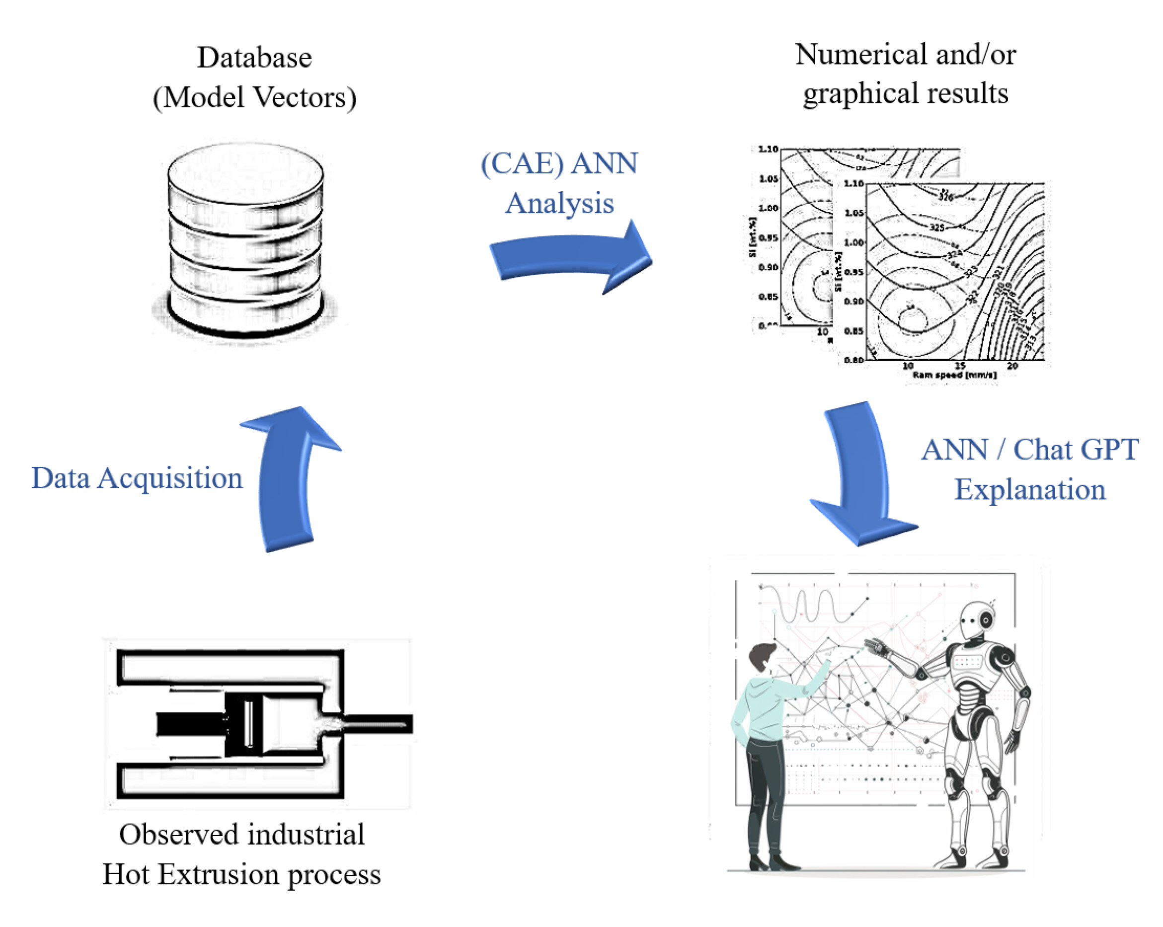
Figure 2.
The microstructure of the extruded round profile of 6082 aluminum alloy: on the edge of extruded profile (a) and in the center of the extruded profile (b).
Figure 2.
The microstructure of the extruded round profile of 6082 aluminum alloy: on the edge of extruded profile (a) and in the center of the extruded profile (b).
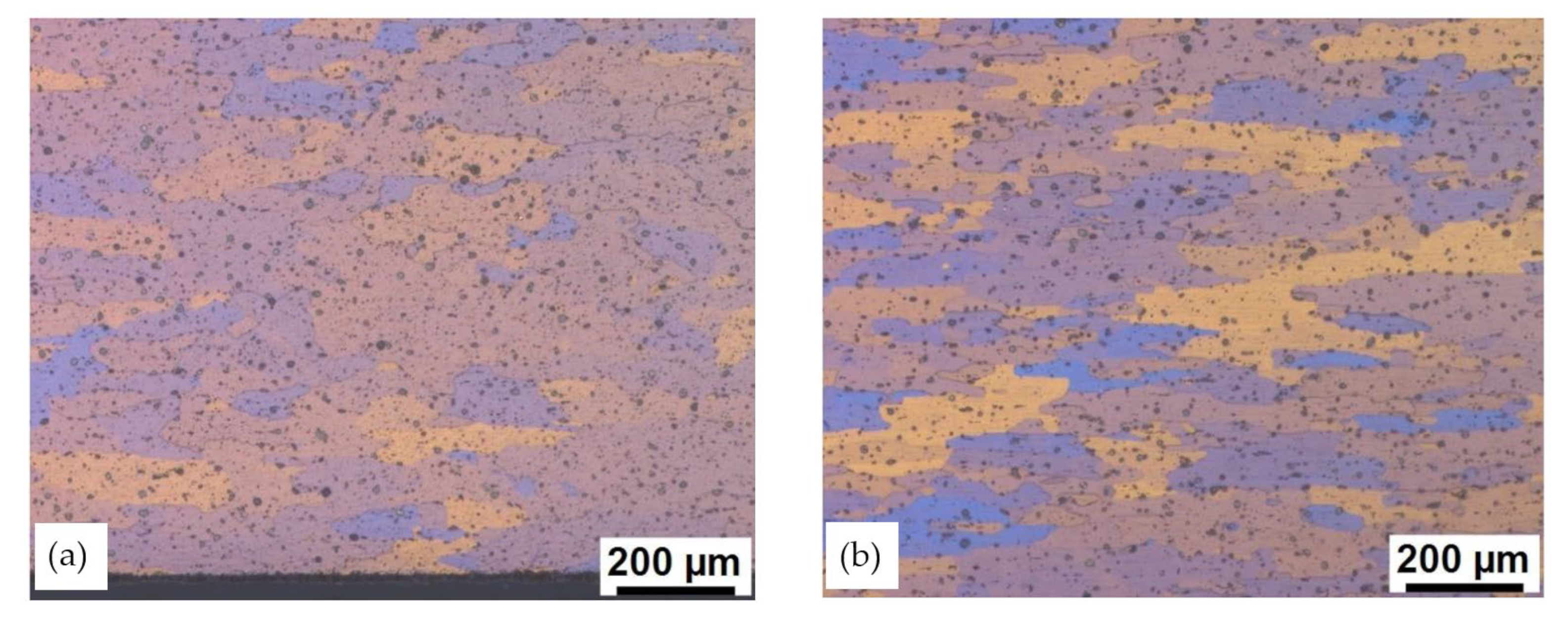
Figure 3.
Prediction of elongation as a function of casting speed (horizontal axis) and Si content: (a) mean value according to Equation (1) and (b) local standard deviation according to Equation (4).
Figure 3.
Prediction of elongation as a function of casting speed (horizontal axis) and Si content: (a) mean value according to Equation (1) and (b) local standard deviation according to Equation (4).

Figure 4.
Prediction of yield strength as a function of casting speed (horizontal axis) and Si content: (a) mean value according to Equation (1) and (b) local standard deviation according to Equation (4).
Figure 4.
Prediction of yield strength as a function of casting speed (horizontal axis) and Si content: (a) mean value according to Equation (1) and (b) local standard deviation according to Equation (4).
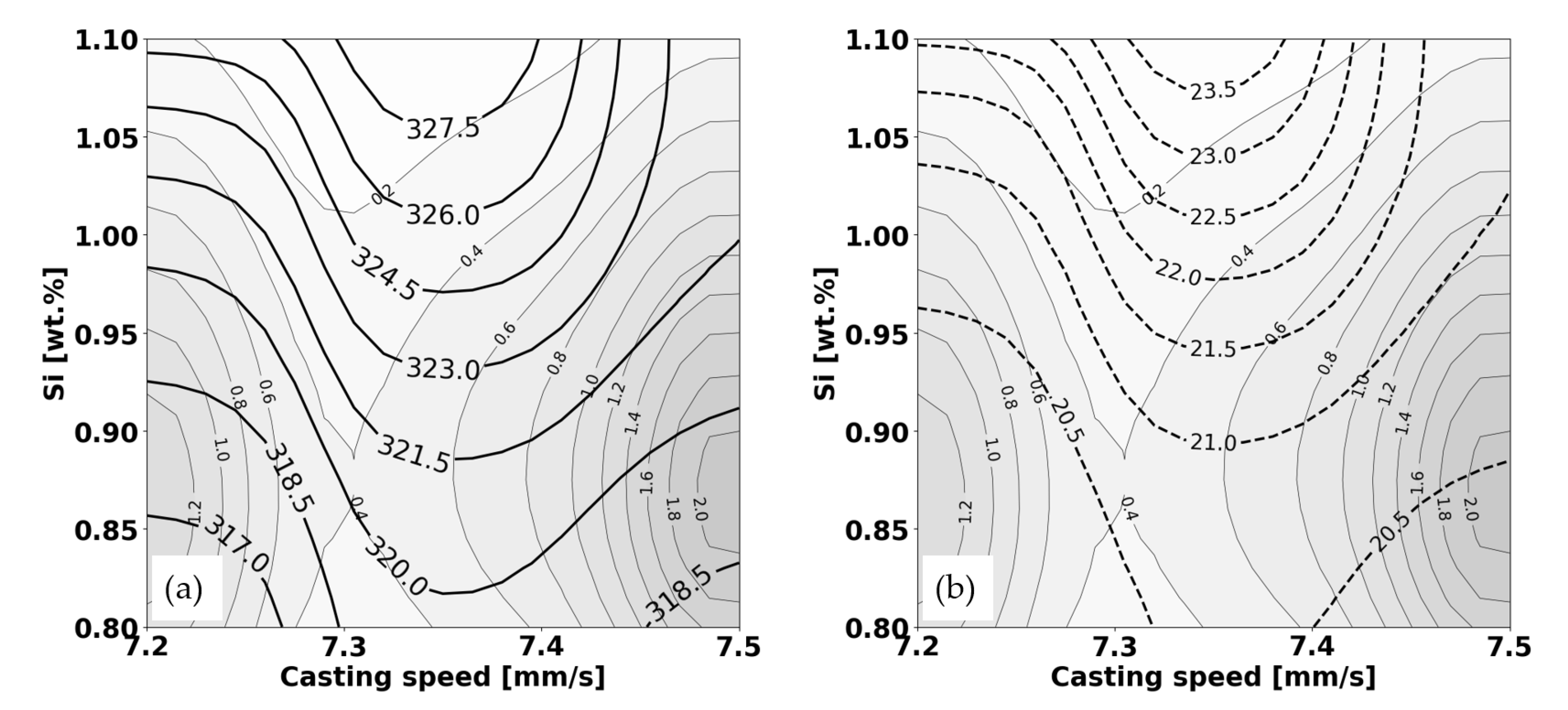
Figure 5.
Prediction of yield strength as a function of casting speed (horizontal axis) and Si content at fixed value of ram speed, which equals 15.405 mm/s: (a) mean value according to Equation (1) and (b) local standard deviation according to Equation (4).
Figure 5.
Prediction of yield strength as a function of casting speed (horizontal axis) and Si content at fixed value of ram speed, which equals 15.405 mm/s: (a) mean value according to Equation (1) and (b) local standard deviation according to Equation (4).
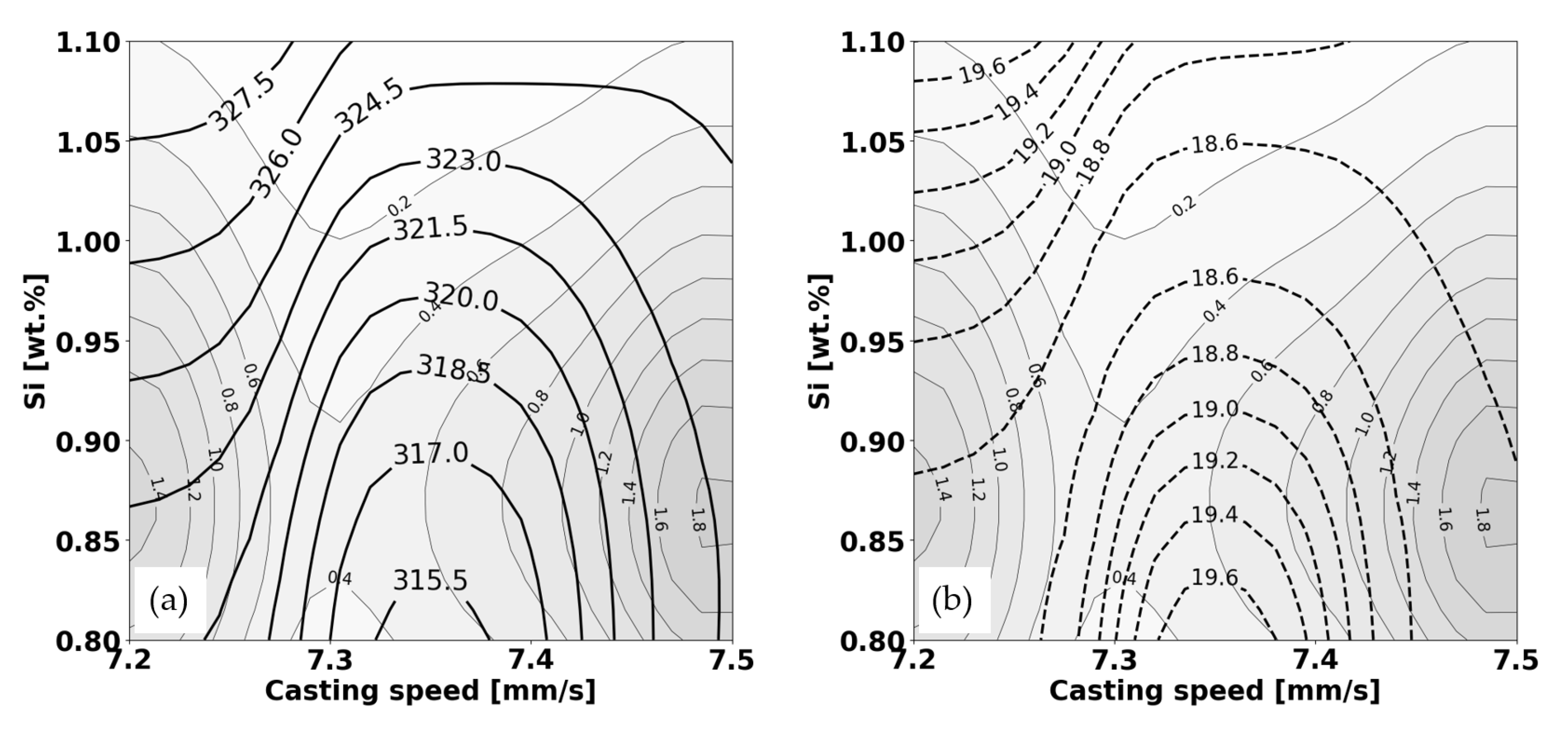
Figure 6.
Prediction of yield strength as a function of casting speed (horizontal axis) and Si content at fixed value of ram speed and Mn content, which equal to 15.471 mm/s and 0.469, respectively: (a) mean value according to Equation (1) and (b) local standard deviation according to Equation (4).
Figure 6.
Prediction of yield strength as a function of casting speed (horizontal axis) and Si content at fixed value of ram speed and Mn content, which equal to 15.471 mm/s and 0.469, respectively: (a) mean value according to Equation (1) and (b) local standard deviation according to Equation (4).
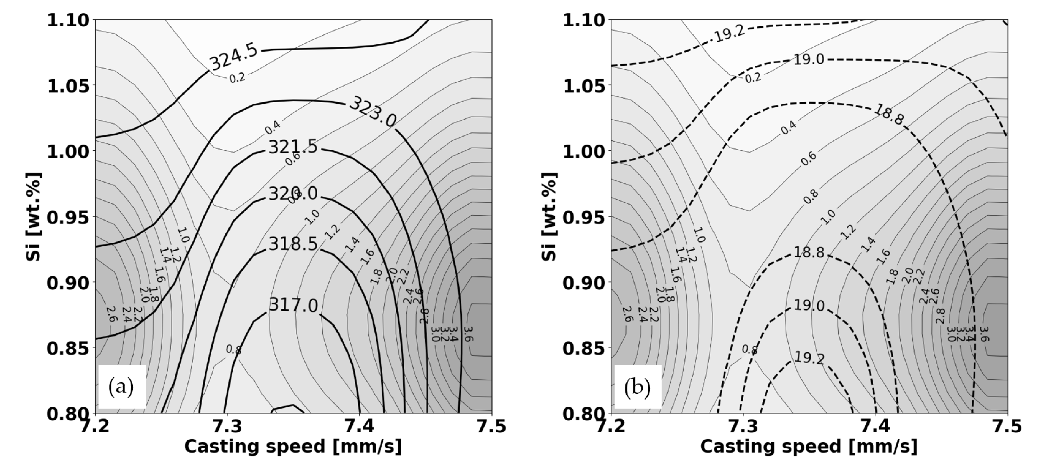
Figure 7.
Prediction of Si content as a function of ram speed (horizontal axis) and Mn content at fixed value of yield strength, which amounts to 322 MPa: (a) mean value according to Equation (1) and (b) local standard deviation according to Equation (4).
Figure 7.
Prediction of Si content as a function of ram speed (horizontal axis) and Mn content at fixed value of yield strength, which amounts to 322 MPa: (a) mean value according to Equation (1) and (b) local standard deviation according to Equation (4).
Disclaimer/Publisher’s Note: The statements, opinions and data contained in all publications are solely those of the individual author(s) and contributor(s) and not of MDPI and/or the editor(s). MDPI and/or the editor(s) disclaim responsibility for any injury to people or property resulting from any ideas, methods, instructions or products referred to in the content. |
© 2024 by the authors. Licensee MDPI, Basel, Switzerland. This article is an open access article distributed under the terms and conditions of the Creative Commons Attribution (CC BY) license (http://creativecommons.org/licenses/by/4.0/).
Copyright: This open access article is published under a Creative Commons CC BY 4.0 license, which permit the free download, distribution, and reuse, provided that the author and preprint are cited in any reuse.


