Submitted:
15 March 2024
Posted:
15 March 2024
You are already at the latest version
Abstract
When the epipelic algae group growing on the concrete inclined side wall, which is typical of urban rivers and open diversion channels, enters the water flow, it will seriously affect the func-tion of the rivers or the channels. It is urgent to predict the transport capacity of epipelic algae group with water flow. However, the current research on the transport of pollutants is mostly based on mathematical models, and the study of the transport of flake epipelic algae group is extremely rare. A generalized hydrodynamic experimental model of a flume with sidewall epi-pelic algae group was established. Through a series of hydraulic experiments, the physical movement form and transport capacity of the suspended epipelic algae group on the side wall of the channel were studied qualitatively and quantitatively by taking the thickness, sheet size and flow rate of the epipelic algae group as the influencing factors. The key influencing factors of the suspension of epipelic algae are clarified, so as to quantitatively analyze the critical conditions of its suspension. Through flow scheduling, the probability of epipelic algae gathering some-where is increased. It provides a theoretical basis for realizing the long-distance migration of epipelic algae and optimizing the mathematical model.
Keywords:
side wall of open channel
; epipelic algae group
; suspension mechanism
; critical conditions
1. Introduction
With the increasing awareness of human environmental protection and the importance of water resources, the eutrophication of water bodies has been effectively controlled worldwide. However, the epipelic algae groups grown on the concrete of the open channel, such as urban rivers and diversion canals, enter the channel in the form of blocks, which are transported with the water flow and even settled. In the past, researchers paid more attention to how to avoid the growth of epipelic algae, but after investigation and research, it was found that the side wall of the open channel would inevitably grow epipelic algae. At the low flow rate of the channel, the epipelic algae will gradually sink to the bottom of the channel and decay and emit stench, which will affect the water quality and environment. However, at the appropriate flow rate, the epipelic algae can gather after a certain distance of suspension with the water flow. Therefore, if the suspension mechanism and theoretical formula of epipelic algae groups can be clarified, it will help to achieve long-distance transportation through flow scheduling and reduce water quality and environmental pollution.
However, the current research on algae mostly focuses on its growth influencing factors and growth changes in different directions. The related research on the suspension movement of epipelic algae is relatively rare. We collect the relevant research results of sediment and oil and other pollutants diffusion and migration with water flow for reference and analysis, in order to provide a basis for this research. Shang Xuemei et al. [1] used the pollutant transport-diffusion model coupled with the hydrodynamic module to numerically simulate the bearing rate of pollutants in Laizhou Bay, Bohai Bay, Liaodong Bay and the central Bohai Sea (China) after oil diffusion. He Leping and Hu Qijun [2] used Fluent software to establish a three-dimensional simulation model of buried oil pipeline leakage including trenches to simulate the leakage and diffusion process under specific accident scenarios. Huang Hailong [3] adopted a two-dimensional mathematical model of suspended sediment transport to study the relationship between suspended sediment diffusion and water depth and tidal pattern. When the water is shallow or neap tide, suspended sediment is not easy to diffuse, and the increase of sediment concentration and the area of turbid waters with high concentration (sediment concentration increment exceeding 10 mg/L) are larger. Yao Jian [4] established a two-dimensional free surface flow MIKE 21 FM model to simulate the pollutants in the confluence area of a Y-type river in southwest China. The results show that a larger confluence ratio will lead to a wider distribution of pollution zones, a smaller vertical concentration gradient of pollutants, and a longer vertical diffusion distance. At the same time, the increase of confluence ratio will increase the horizontal concentration gradient of pollutants and aggravate the diffusion trend of pollutants at the intersection. Based on the EFDC model, Li Yafeng [5] simulated the diffusion of pollutants that may occur in the reservoir area and the leakage of pollutants from sudden risk accidents in the water. The results showed that the wet year had a great influence on the effluent quality, and the dry year had little effect on the effluent quality. Hou Jingming [6] simulated the pollutant transport process in sudden water pollution accidents based on the GPU accelerated surface water flow and transport model (GAST model), which can quickly and accurately simulate the pollutant transport process in sudden water pollution accidents caused by rainstorm flash floods or dam-break floods. Based on the environmental fluid hydrodynamic model (EFDC), Tao Ya[7] numerically simulated and analyzed the influence range, time and degree of sudden water pollution accidents in Shenzhen Estuary (China) under different hydrological conditions from the perspective of hydrodynamics. Based on the hydrodynamic conditions of Barcelona Port in Spain, Manel et al. [8] simulated and analyzed the degree of influence of different waters under the influence of near-shore tidal current in sudden oil spill pollution accidents, and put forward the control countermeasures to deal with the deterioration of water quality. Sun Sanxiang [9] studied the transport of pollutants by establishing a transport model of pollutants in runoff on the underlying surface covered by plants. The results showed that the concentration of pollutants in runoff had an exponential relationship with the effective rainfall depth. Yang Zhonghua [10] used Lagrange's random displacement model to set different vegetation densities and the probability of river bed absorption of pollutants. The transport process of instantaneously released pollutants in wetlands with dense rigid submerged vegetation and riverbed absorption boundary is simulated.
At present, the main research method of suspension is mathematical model. However, in view of the fact that the mathematical model cannot fully simulate the biochemical characteristics of the main body of suspension, we directly used the epipelic algae whose bulk density and thickness are close to the prototype in the previous hydrodynamic test research. By changing the flow level, algae thickness and algae size, the generalized model test of suspension of epipelic algae group was carried out. The form of the transport movement of the epipelic algae in the water is counted, and its transport capacity with the water flow was analyzed, and the key parameters of its transport were quantified, and the model was verified at the same time. It provides a strong theoretical basis for the comprehensive analysis of later mathematical model calculation.
2. Materials and Methods
On the basis of the flume of the previous experimental study on the hydrodynamics of the epipelic algae on the side wall of the open channel [11], the longitudinal slope is 1:26000, the slope of the side wall is 1:2.5, the maximum water flow is 420m3/s, and the generalization is carried out according to the scale of 1:30. According to the flow of the prototype channel, the size of the epipelic algae, the sediment and algae content in the algae group were simulated (Figure 1). We selected 40 groups of epipelic algae sizes and 5 groups of different flow rates to carry out the test.
The flow stabilization measures are set up in the forebay of the flume (Figure 2). According to the gravity similarity, resistance similarity criterion and water flow continuity, the Froude number similarity condition is used to calculate the scale of flow velocity, flow rate and time. The test instrument adopts the propeller current meter (accuracy 0.01 m/s) and the electromagnetic flowmeter (accuracy 0.01 L/s).
The previous results [11] show that the position of the maximum velocity on the vertical line of the channel flow appears at a relative water depth of 0.6.Therefore, the current meter is installed at a relative water depth of 0.6 in the center of the flume to measure the mainstream velocity of the flume.
3. Results
3.1. Physical Figure of Suspension of Epipelic Algae Group
Through multiple sets of test results, it is found that the epipelic algae group is taken away by the water flow at the moment of shedding, and the critical hydrodynamic state of suspension is the critical hydrodynamic state of shedding. However, due to the internal effects of physical and chemical properties such as the thickness, size and growth cycle of the epipelic algae group, there may be a lag of suspension compared with the mainstream of the channel. In general, the suspension state after the epipelic algae group enters the water flow is divided into: flip suspension, no flip suspension, aggregation transport, settlement transport and other forms, and its suspension state is directly related to the main flow rate and flow rate of the channel.
When the flow rate is 102.04 m3/s, the small-scale epipelic algae groups can be easily taken away by the water flow (Figure 3). Although the forms of suspension of epipelic algae are different, they can flip, settle, or float on the water surface, but they can all be brought downstream with the water flow. The difference is the time taken to the downstream. The transport form of flipping and settling takes a long time, which has obvious hysteresis compared with the suspension mode floating on the water surface.
When the flow rate is 220.84 m3/s, the shed epipelic algae is also transported downstream with the water flow in the form of flipping, settling, and floating on the water surface (Figure 4). With the increase of the flow rate, the time taken by the flipping and floating on the water surface to the downstream is almost the same. However, the form of re-transport after sedimentation takes a long time to move downstream and it still has obvious hysteresis.
When the flow rate is 301.69 m3/s, most of the shed epipelic algae are transported downstream in the form of suspended on the water surface, and only a very small amount of epipelic algae with a thickness of 8mm first settles and then transports downstream (Figure 5). Therefore, we believe that as the flow rate increases, the flow velocity increases, and the mainstream of the water flow has a stronger suspension effect on the epipelic algae group.
According to the physical graphics of the turnover, settlement and floating of the epipelic algae group on the water surface (Figure 6), in order to reduce the water pollution caused by the shedding and settlement of the epipelic algae group, the law of easy suspension and less settlement should be followed in the large flow rate and small scale of the epipelic algae group. In the early stage of the growth of the epipelic algae, the flow rate should be increased to reduce the settlement of the epipelic algae group.
3.2. Establishment of the Critical Theoretical Formula for the Suspension of Epipelic Algae Group
3.2.1. Analysis of Transport Capacity of Epipelic Algae Group
The epipelic algae group that enters the channel flow after shedding is studied as a relatively independent medium in the water body. It is of great significance to study the mechanical mechanism of transport and the transport capacity of water flow to improve the hydrodynamic conditions and control water pollution through the main canal scheduling. Based on the pollutant migration theory of environmental hydraulics, the drift of the epipelic algae into the water body with the water flow is regarded as the flow of the epipelic algae into the water body. The resistance of epipelic algae in water flow can be referred to the Stokes formula of viscous resistance. This viscous resistance is the basis for analyzing the transport capacity of water flow to epipelic algae under different water flow conditions.
At present, the more mature researches are the study of the resistance of algae groups in the flow of small Reynolds number. Scholars believe that the particle size of common algae groups and the relative velocity between fluid and particles are very small. Therefore, the particle flow model is used to analyze the force of algae groups in the flow. The flow around the particles is a typical small Reynolds number flow, and the Stokes formula of the viscous resistance is:
In which, W is the viscous resistance; μ is the viscosity of water; V' is the relative velocity of algae in water; r is the radius of algae group.
The formula (1) is to particleize the algae and analyze it. In view of the fact that the scale of the epipelic algae group is very small relative to the whole channel, there is a velocity difference between the fluid and the algal group related to the density of the algae group. Therefore, we introduce the velocity difference coefficient f(ε) related to the density of the algae to correct V'. At the same time, the lamellae of the algae group are quantified as the size of the sphere particles. Because the algae group has a thickness, we convert its volume into the volume of the body sphere.
In which, l is the length of algae group; w is the width of algae group, δ is the thickness of algae group.
The parameter z is introduced to represent the radius of the epipelic algae ball:
Then the Stokes formula of viscous resistance is transformed into:
The formula (4) shows that the viscous resistance of the water body is directly related to the relative velocity in the water body and the size of the epipelic algae group, but it is not directly proportional to the relationship, and the specific quantitative relationship still needs further study.
When the epipelic algae group is washed off from the side wall by the water flow, whether the water flow has an effective transport effect on the epipelic algae group can be determined by analyzing the followability of the algae group in the water body. The density of common algae groups in rivers and lakes is basically the same as that of water bodies. Therefore, it can be considered that the buoyancy and gravity of algae groups offset each other, and the biological resistance of algae groups is ignored. It is considered that algae groups are mainly affected by the viscous resistance of fluid in water flow. However, due to the biochemical effect of the sediment and algae on the side wall of the channel, it cannot be ignored. Some epipelic algae float on the water surface and transport at the same speed with the water flow, while some algae enter the water body and continue to transport under the longitudinal action of the water flow. The density of water and algae is recorded as ρ. If the main flow velocity of water is V0 and the instantaneous velocity of an isolated algae group in water is V, then the relative velocity of algae group and water flow is V′ = V0 - V. According to the formula (4) of the viscous resistance of the algae group, the acceleration of the algae group is:
Where
In which, a is the acceleration of the algae group; υ is the kinematic viscosity coefficient of water; m is the mass of algae group.
The instantaneous velocity V of the algae group satisfies:
The formula (7) shows that under the action of viscous resistance of water flow, the instantaneous velocity of the epipelic algae group approaches the mainstream velocity V0 with the increase of time t.
The smaller the size of the epipelic algae group, the shorter the time it takes to catch up with the mainstream velocity, the better the followability of the epipelic algae group, and the more obvious the effect of water flow on the algae group. Through experimental research, it can be obtained (Table 1): When the velocity V of the algae group reaches more than 95% of the main flow velocity V0, it can be considered that the algae group has all moved forward with the water flow without relative lag, that is, it is suspended on the water surface. If it reaches 95%~85% of the main flow velocity, it is considered that the algae group is lagging behind, that is, it is transported with the water flow below the water surface. If it reaches 85%~80% of the main flow velocity, it is first settled and then transported with the water flow. If it is lower than 80% of the main flow rate, with the increase of time, the epipelic algae group is likely to stop moving after a certain distance, which will cause the epipelic algae group to accumulate at the bottom of the channel and cause water metamorphism.
3.2.2. Analysis of Influencing Factors on the Transport Velocity of Epipelic Algae Group and Verification of Model Test
The transport velocity of the epipelic algae group is mainly related to the average flow velocity of the mainstream (flow rate), the thickness of the algae, the size of the algae (area), and the shape. The various factors are analyzed below.
(1) The effect of the average flow velocity of the mainstream on the transport velocity of epipelic algae group
The experiment mainly considered the effects of five mainstream average flow velocities of 1.25 m/s, 1.36 m/s, 1.48 m/s, 1.75 m/s and 1.89 m/s on the transport velocity of epipelic algae group. The smaller the average flow velocity of the mainstream, the smaller the transport velocity of the epipelic algae group. When the average flow velocity of the mainstream is 0 m/s, the transport speed of the epipelic algae group should also be 0 m/s; the larger the average flow rate of the mainstream, the greater the transport speed of the epipelic algae group, and the transport velocity of the epipelic algae group generally does not exceed the average flow velocity of the mainstream. The transport velocity of the epipelic algae group is basically linear with the average flow velocity of the mainstream (Figure 7). Therefore, it can be obtained that:
In which, V is the transport velocity of epipelic algae group; a1 is a parameter, which should be in (0, 1); V0 is the average flow velocity of the mainstream.
(2) The effect of algae thickness on the transport velocity of epipelic algae group
The experiment mainly considered the influence of the thickness of 3mm, 6mm and 8mm on the transport velocity of epipelic algae group. The smaller the thickness of the algae, the greater the transport velocity of the epipelic algae group, and the transport velocity of the epipelic algae group is inversely related to the thickness of the algae. The transport velocity of the epipelic algae group is basically linear with the thickness of the algae (Figure 8). Therefore, it can be obtained that:
In which, V is the transport velocity of epipelic algae group; a2, a3 are parameters greater than 0; δ is the thickness of algae group.
(3) The effect of algae area on the transport velocity of epipelic algae groups
The influence of the shape and area of nine kinds of algae group (3m × 3m, 6m × 3m, 6m × 6m, 9m × 6m, 9m × 9m, 15m × 15m, 21m × 15m, 18m × 18m, 30m × 18m) on the transport velocity of epipelic algae group was mainly considered in the experiment.
The smaller the area of the algae, the greater the transport velocity of epipelic algae group, and the transport velocity of epipelic algae group is inversely related to the area of the algae group. The transport velocity of epipelic algae group is basically linear with the area of algae (Figure 9). However, there is also a quadratic relationship. When the mainstream flow velocity is below 1.48 m/s, with the increase of area, the transport velocity of epipelic algae group has an accelerated downward trend. When the mainstream flow velocity is below 1.75 m/s, with the increase of area, the downward trend of the transport velocity of epipelic algae group may slow down and may rise. Therefore, it can be obtained that:
In which, V is the transport velocity of epipelic algae group; a4, a5, a6, a7 are parameters greater than 0, a4 is a very small number, and a5 should be in (1.48, 1.75); V0 is the average flow velocity of the mainstream; A is the area of algae group.
From the above, we can conclude that:
The values of a1, a2, a3, a4, a5, a6 and a7 were obtained by fitting, and the formula for calculating the transport velocity of epipelic algae group is obtained by bringing into the relationship:
4. Discussions
4.1. Research Results of Longitudinal Transport Velocity along the Sidewall
Based on the Mike21 model, Sun Zhaohua [12] established a two-dimensional hydrodynamic-water quality model to study the changes of water level and flow velocity and self-purification ability after sudden water pollution accidents in the vicinity caused by the arrangement of different density wharf groups. The differences among the three changes are compared from the perspectives of spatial difference and maximum amplitude, and the relationship among wharf density and hydrodynamic conditions and pollutant concentration amplitude is summarized. The results show that the concentration of the mainstream area in the project area increases, the concentration of the near-shore zone decreases, and the overall retention time of the high concentration increases. Ren Chunping [13] studied the horizontal two-dimensional transport and diffusion characteristics of pollutants through physical model tests. The results showed that pollutants were mainly transported along the sidewall direction, and the transport speed in the vertical sidewall direction was less than that along the sidewall direction. The results of this study show that the transport of epipelic algae has a certain lag relative to the mainstream of the channel. This is because the longitudinal transport along the sidewall is the main trend of the transport of mud algae when the epipelic algae group enters the water flow in the early stage. After a short period of lateral transport and sidewall transport, it is transformed into the longitudinal transport of the mainstream. We believe that there is no effect of concentration and water dilution in this study, but the results are consistent with the research results of other scholars.
4.2. Study on the Influence of Wind on Transport
Shu Yehua [14] established a high-precision three-dimensional wind-induced current numerical model and wind-induced current-pollutant coupling numerical model of Taihu Lake (China), and analyzed the characteristics of wind-induced current in Taihu Lake under the action of prevailing wind and the characteristics of pollutant transport in Taihu Lake driven by wind-induced current. The results show that the surface velocity of the stable wind-induced flow field in Taihu Lake is greater than the bottom velocity, and the surface flow direction is basically the same as the wind direction, while the bottom flow direction is roughly opposite to the surface, with the characteristics of compensation flow. Wind direction can significantly affect the morphology and structure of wind-driven current in Taihu Lake. Huilin Wang and Wenxin Huai [15] considered that both surface wind and bed absorption have an important influence on the pollutant diffusion process. Considering these two factors, a multi-scale method was used to describe the environmental diffusion process in wetland flow. The results of the proposed multi-scale method are in good agreement with the data set generated by the numerical method.
Zhao Guixia and Gao Xueping [16] studied the influence of wind-induced lateral disturbance on the horizontal migration and aggregation of algae in the lake. There are significant differences in the influence of different wind directions on the horizontal transport of algae. Overall, the wind field changed the spatial distribution of algae residence time in the lake area. From the perspective of spatial distribution, the influence of wind field on algae residence time is most significant in the middle and lower reaches, but not significant in the middle and upper reaches. In addition, the wind field effectively enhanced the migration connectivity of algae in the lake. The migration connectivity between the algae in the lake and the upstream of the source area increased with the increase of the wind field, and the migration connectivity with the downstream of the source area increased with the increase of the wind field intensity and the distribution is more uniform. Scholars have studied the influence of wind on transport from different angles. In this study, because it is an indoor generalized model test, combined with the results of field investigation, the effect of wind on the transport of epipelic algae group is attributed to the effect of wind on water flow, and the water flow then forms the transport of epipelic algae group. In addition, the scale of epipelic algae group is larger than that of pollutants, so the effect of wind is no longer considered separately.
4.3. Study on the Influence of Water Flow Characteristics on Transport
Zhu Jinge [17] studied the variation characteristics of pollutant transport rate in the western Taihu Lake (China). The results showed that the input rates of nitrogen and phosphorus in Chengdong Port were controlled by concentration, and the transport rates of other rivers were controlled by flow rate. Zhang Yinghao and Lai Xijun [18] used the energy spectrum distribution of instantaneous velocity to separate wave velocity from turbulent velocity, and analyzed the effects of aquatic plants on time-averaged velocity, wave velocity and turbulent kinetic energy respectively. In order to study the transport capacity of water flow to algal blooms, Ji Daobin [19] generalized algal blooms into material particles in water bodies. Studies have shown that water flow can produce significant push flow transport effects on algal blooms. Scholars regard water flow velocity, kinetic energy and density flow as the main factors affecting transport, which is consistent with the results of this study.
4.4. Research Results of Gathering Place Prediction
Magdalena Musielak et al. [20] used the immersed boundary method to simulate the interaction of rigid and flexible diatom chains with surrounding fluids and nutrients. Galabov et al. [21] took the oil tanker accident in the Gulf of Burgas as an example, used the numerical simulation method to analyze the pollutants drifting on the sea surface, evaluated the impact of the oil spill accident on the water environment risk of the Port of Burgas, and determined the potential dangerous area and its occurrence conditions. Due to the great environmental impact of pollutants and epipelic algae on rivers, lakes and oceans, if the pollutant accumulation prediction can be carried out according to its transport characteristics, active measures will be taken to effectively reduce the impact on the environment. Scholars have predicted potential dangerous areas by mathematically simulating the interaction of pollutants with water flow and water environmental risk assessment, and have not established a quantitative relationship. The purpose of this study is to establish a transport formula through physical model tests, and to predict the gathering place of epipelic algae group. The research methods are different, but this physical model will provide a research basis for the continuous optimization of mathematical models in the later period.
5. Conclusions
The experimental study on the suspension of the epipelic algae group on the side wall of the open channel in the water flow shows that:
(1) The epipelic algae has many forms of flip suspension, no flip suspension, aggregation transport and settlement transport, and its suspension state is directly related to the main flow velocity and flow rate of the channel.
(2) When the velocity V of the algae group reaches more than 95% of the main flow velocity V0, it can be considered that the algae group has all moved forward with the water flow without relative lag, that is, it is suspended on the water surface. If it reaches 95%~85% of the main flow velocity, it is considered that the algae group is lagging behind, that is, it is transported with the water flow below the water surface. If it reaches 85%~80% of the main flow velocity, it is first settled and then transported with the water flow. If it is lower than 80% of the main flow rate, with the increase of time, the epipelic algae group is likely to stop moving after a certain distance.
(3) The hydrodynamic formula of epipelic algae suspension was established, and the formula was verified by experimental data. The results showed that the formula calculation and the data were in good agreement.
Author Contributions
Conceptualization, M.Z.; methodology, L.P.; validation, Z.W.; formal analysis, G.W.; investigation, Y.Z.; resources, L.P.; data curation, L.P.; writing—original draft preparation, L.P.; writing—review and editing, M.Z.; supervision, Z.L.; project administration, L.P.; funding acquisition, Z.L. All authors have read and agreed to the published version of the manuscript.
Funding
This research was funded by the Excellent Youth Science Fund of Henan Province, grant number 232300421065, the Natural Science Foundation of Henan Province, grant number 212300410200, the Beijing Jianghe Water Development Foundation, Young Talents of Water Con-servancy Science and Technology Fund Support, grant number YC202306, the Key Commonwealth Project of Henan Province, grant number 201300311600, the Basic Research and Development Special Fund of Central Government for Non-profit Research Institutes, grant number HKY-JBYW-2023-10, HKY-JBYW-2020-05.
Institutional Review Board Statement
Not applicable.
Informed Consent Statement
Not applicable.
Data Availability Statement
The data presented in this study are available on request from the corresponding authors.
Acknowledgments
We would like to thank the potential reviewer very much for their valuable comments and suggestions. We also thank my other colleagues’ valuable comments and suggestions that have helped improve the manuscript.
Conflicts of Interest
The authors declare no conflict of interest.
References
- Shang Xuemei, Lou Angang, Sun Xuejuan, et al. Numerical simulation of petroleum hydrocarbons transport in Bohai Sea and the influences on water quality. Marine Environmental Science, 2015, 31, 58–65. [Google Scholar]
- He Leping, Wang Zefan, Hu Qijun, et al. On the oil leakage and diffusion regularity for the underground buried oil pipelines. Journal of Safety and Environment, 2019, 19, 1232–1239. [Google Scholar]
- Huang Hailong, Wang Zhen. Numerical analysis of suspended sediment diffusion caused by underwater excavation. Port & Waterway Engineering, 2015, 505, 25–35. [Google Scholar]
- Mi Tan, Yao Jian. Simulation of Pollutant Diffusion in Y-type River Confluence. Environmental Science & Technology, 2020, 43, 9–16. [Google Scholar]
- Li Yafeng, Wu Jianbo, Cheng Hao. Simulation of Pollutant Diffusion in Tanghe Reservoir Based on EFDC Model. Journal of Shenyang Jianzhu University (Natural Science), 2022, 38, 945–952. [Google Scholar]
- Shi Baoshan, Hou Jingming, Wang Junhui, et al. Simulation of pollutant transport in sudden water pollution accident based on GAST model. Engineering Journal of Wuhan University, 2022, 55, 1112–1119. [Google Scholar]
- Tao Ya, Lei Kun, Xia Jianxin. Main hydrodynamic factors identification for pollutant transport in sudden water pollution accident in Shenzhen Bay. Advances in Water Science, 2017, 28, 888–897. [Google Scholar]
- Manel G, Gabriel J, Manuel E, et al. A management system for accidental water pollution risk in a harbor: the Barcelona case study. Journal of Marine Systems 2011, 88, 60–73. [CrossRef]
- Li Haifeng, Sun Sanxiang. Experimental study on the transport characteristics of pollutants on the underlying surface covered by plants. Yellow River, 2023, 45, 79–81. [Google Scholar]
- Fang Haoze, Yang Zhonghua. Effects of submerged vegetation and bed absorption boundary on pollutant transport in wetland. Advances in Water Science, 2023, 34, 126–133. [Google Scholar]
- Pan Li, Zhao Lianjun, Zhang Mingwu, et al. Experimental Study of the Hydrodynamics of an Open Channel with Algae Attached to the Side Wall. Water, 2023, 15, 2921. [Google Scholar] [CrossRef]
- Xiong Haibin, Sun Zhaohua, Chen Li, et al. Analysis of the Effects of Varying Density in Wharf Groups on River Hydrodynamics and Pollutant Transport: A Case Study in Wuhan Reach. Resources and Environment in the Yangtze Basin, 2021, 30, 2205–2216. [Google Scholar]
- Yu Chong, Ren Chunping. An experimental study on horizontal two-dimensional transport and diffusivity of dye under irregular waves in surf zone. Marine Environmental Science, 2021, 40, 34–40. [Google Scholar]
- Shu Yehua, Gao Chenchen. Numerical simulation of wind-driven current and pollutant transport and diffusion in Taihu Lake. Water Resources Protection, 2021, 37, 120–127. [Google Scholar]
- Wang Huilin, Li Shuolin, Zhu Zhengtao, Huai Wenxin. Analyzing solute transport in modeled wetland flows under surface wind and bed absorption conditions. International Journal of Heat and Mass Transfer, 2020, 30, 1–12. [Google Scholar]
- Zhao Guixia, Gao Xueping. Influence of turbulent disturbance on algae in the large shallow lake; Tianjin University: Tianjin, China, 2020; pp. 1–161. [Google Scholar]
- Zhu Jinge, Liu Xin, Deng Jiancai, et al. Pollutant transport rates in the rivers around western Lake Taihu. Journal of Lake Sciences, 2018, 30, 1509–1517. [Google Scholar] [CrossRef]
- Zhang Yinghao, Lai Xijun, Zhang Lin, et al. Influence of aquatic vegetation on flow structure under wind-driven waves: a case study in Lake Taihu (China) with two typical submerged vegetations. Advances in Water Science, 2020, 31, 441–449. [Google Scholar]
- Ji Daobin, Li Guojing, Yang Zhengjian, Ma Jun, Huang Yuling, Liu Defu. Water Transport Capacity for Algal Bloom in Tributaries of Three Gorges Resevoir. Water Resources and Power, 2013, 31, 75–77. [Google Scholar]
- Magdalena M, Musielak, Leekarp-Boss, et al. Nutrient transport and acquisition by diatom chains in a moving fluid. Journal of Fluid Mechanics 2009, 638, 401–421. [CrossRef]
- Galabov V, Kavortche A, Marinski J. Simulation of tanker accidents in the bay of Burgas, using hydrodynamic model. Proceedings of the International Multidisciplinary Scientific GeoConference Surveying, Geology and Mining, Ecology and Management, 2012, 3. [Google Scholar]
Figure 1.
The epipelic algae with the same sediment and algae content as the prototype.

Figure 2.
Schematic diagram of generalized model test: (a) Plan view of model circulation system; (b) Cross section of generalized model test; (c) Photograph of flume.
Figure 2.
Schematic diagram of generalized model test: (a) Plan view of model circulation system; (b) Cross section of generalized model test; (c) Photograph of flume.
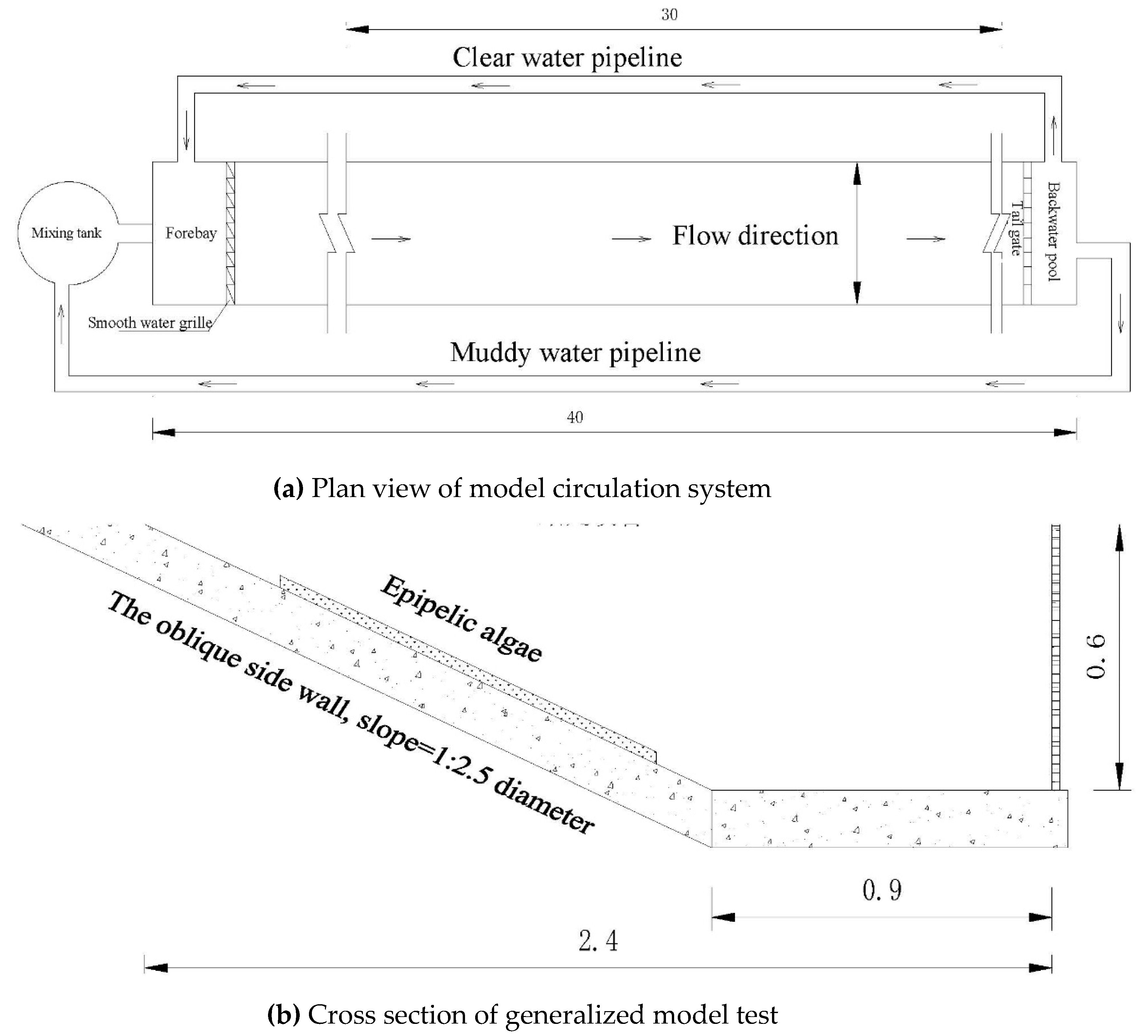
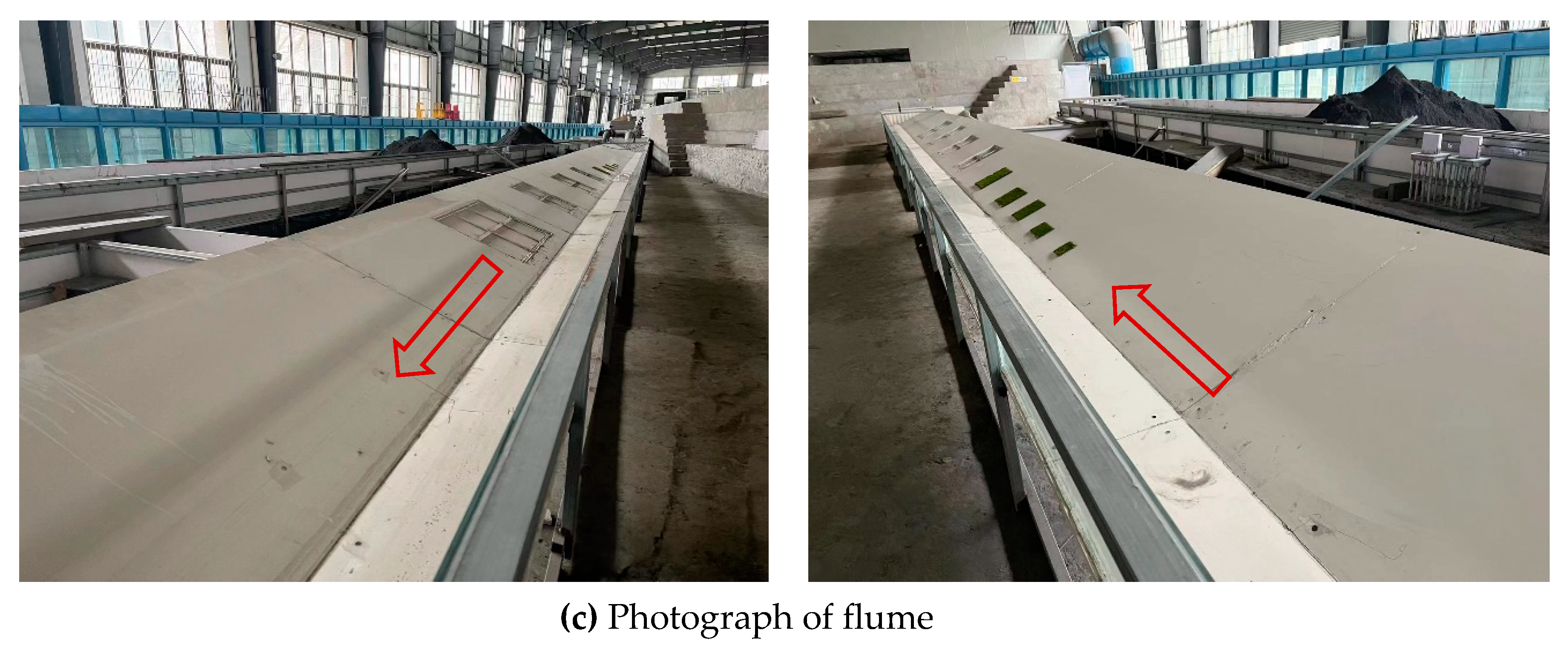
Figure 3.
The transport form of epipelic algae group at Q=102.04 m3/s.
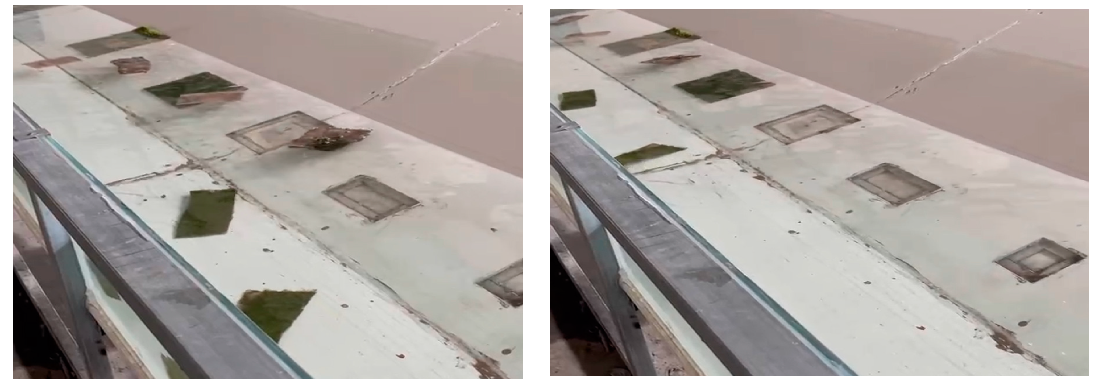
Figure 4.
The transport form of epipelic algae group at Q=220.84 m3/s.
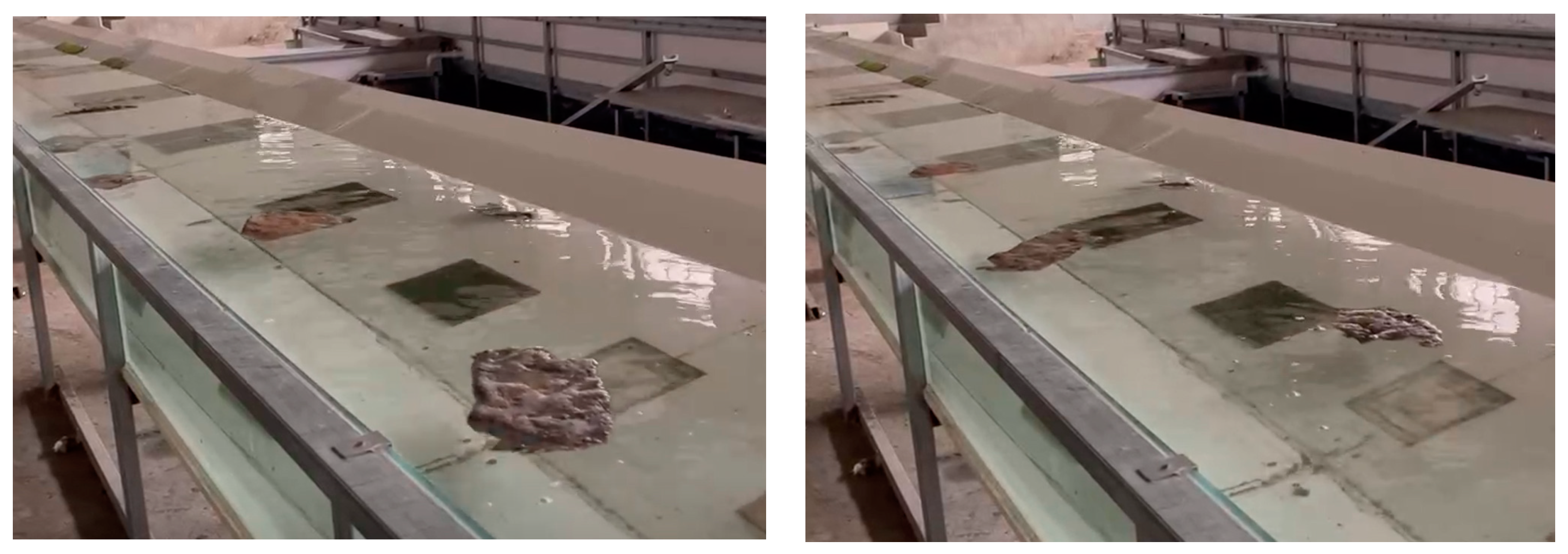
Figure 5.
The transport form of epipelic algae group at Q=301.69 m3/s.
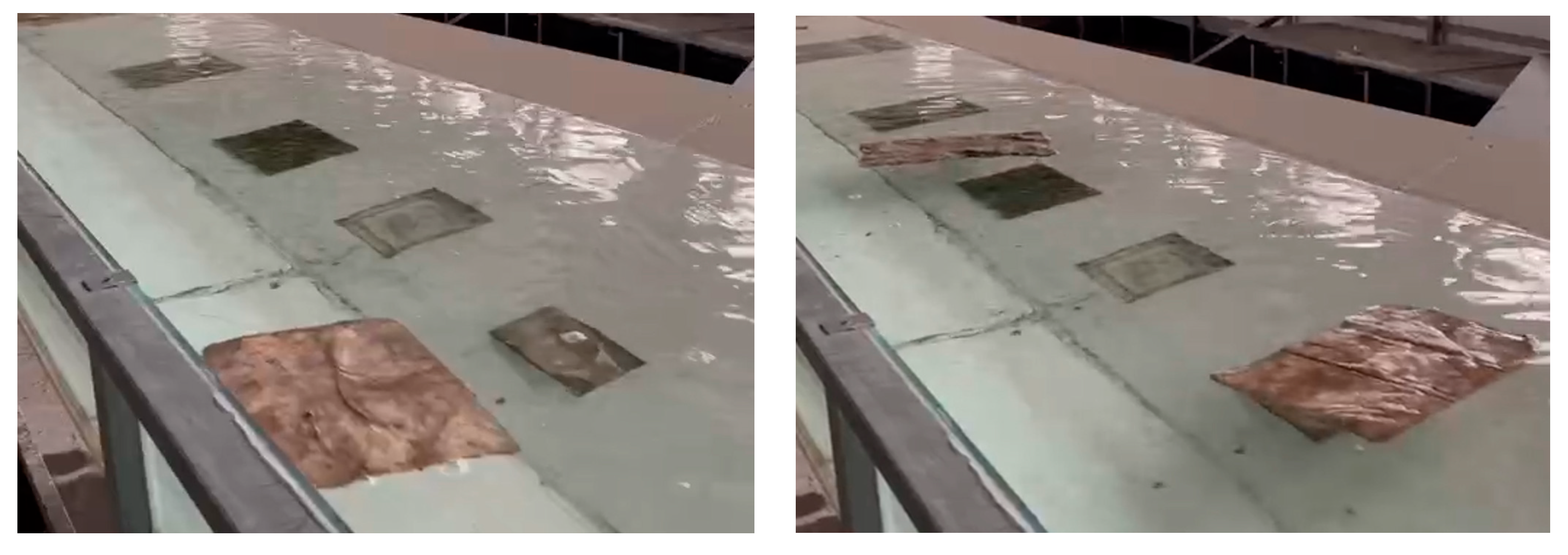
Figure 6.
Physical figure of suspension of epipelic algae group.
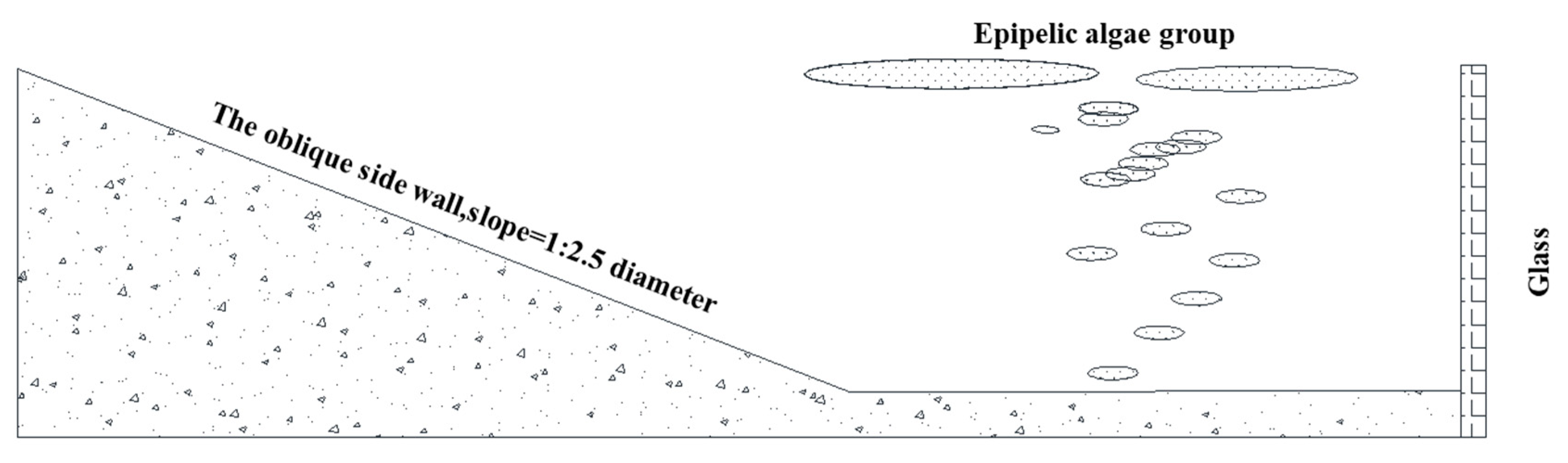
Figure 7.
Transportation of different sizes of epipelic algae group: (a) a × b = 3 m × 3 m; (b) a × b = 6 m × 3 m; (c) a × b = 9 m × 9 m; (d) a × b = 15 m × 15 m; (e) a × b = 21 m × 15 m; (f) a × b = 30 m × 18 m.
Figure 7.
Transportation of different sizes of epipelic algae group: (a) a × b = 3 m × 3 m; (b) a × b = 6 m × 3 m; (c) a × b = 9 m × 9 m; (d) a × b = 15 m × 15 m; (e) a × b = 21 m × 15 m; (f) a × b = 30 m × 18 m.
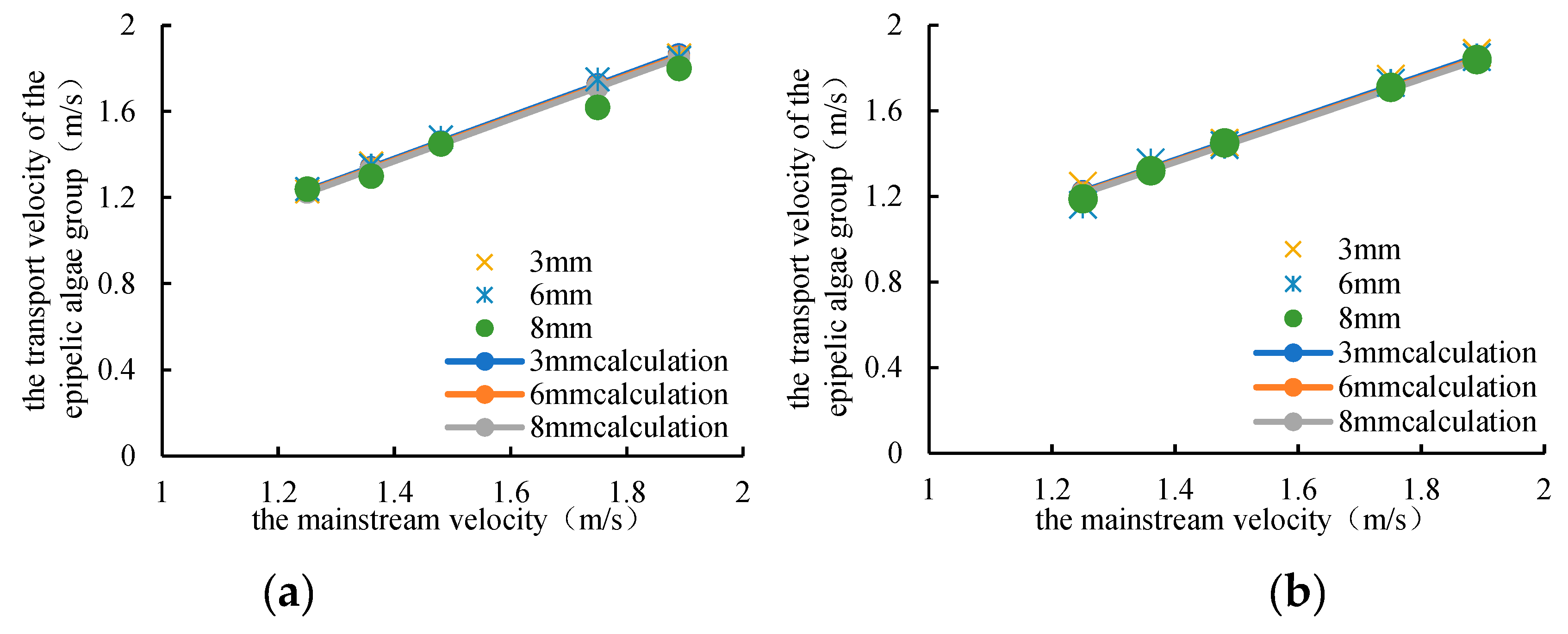
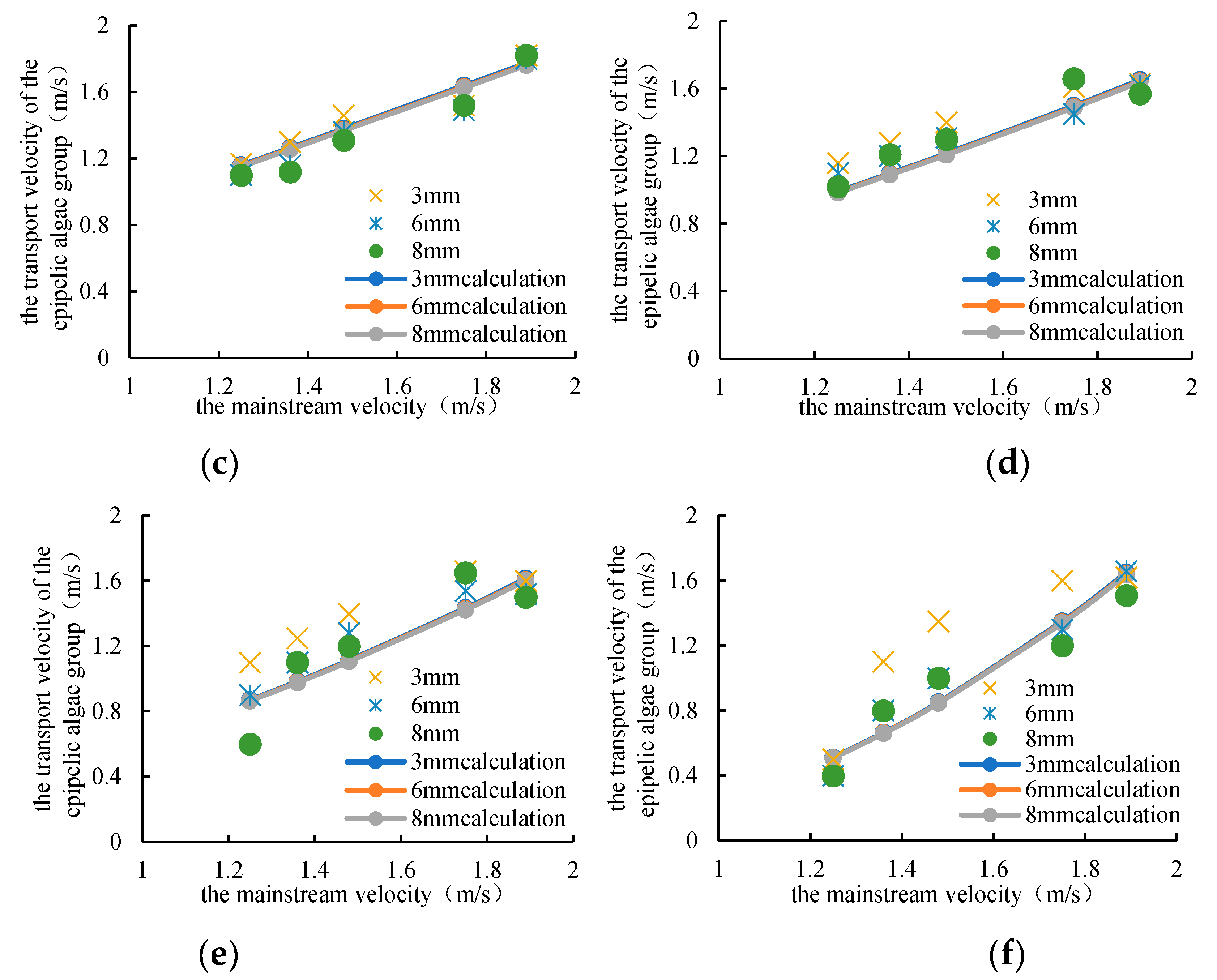
Figure 8.
Transportation of different thickness of epipelic algae groups: (a) a × b = 3 m × 3 m; (b) a × b = 6 m × 3 m; (c) a × b = 9 m × 9 m; (d) a × b = 15 m × 15 m; (e) a × b = 21 m × 15 m; (f) a × b = 30 m × 18 m.
Figure 8.
Transportation of different thickness of epipelic algae groups: (a) a × b = 3 m × 3 m; (b) a × b = 6 m × 3 m; (c) a × b = 9 m × 9 m; (d) a × b = 15 m × 15 m; (e) a × b = 21 m × 15 m; (f) a × b = 30 m × 18 m.
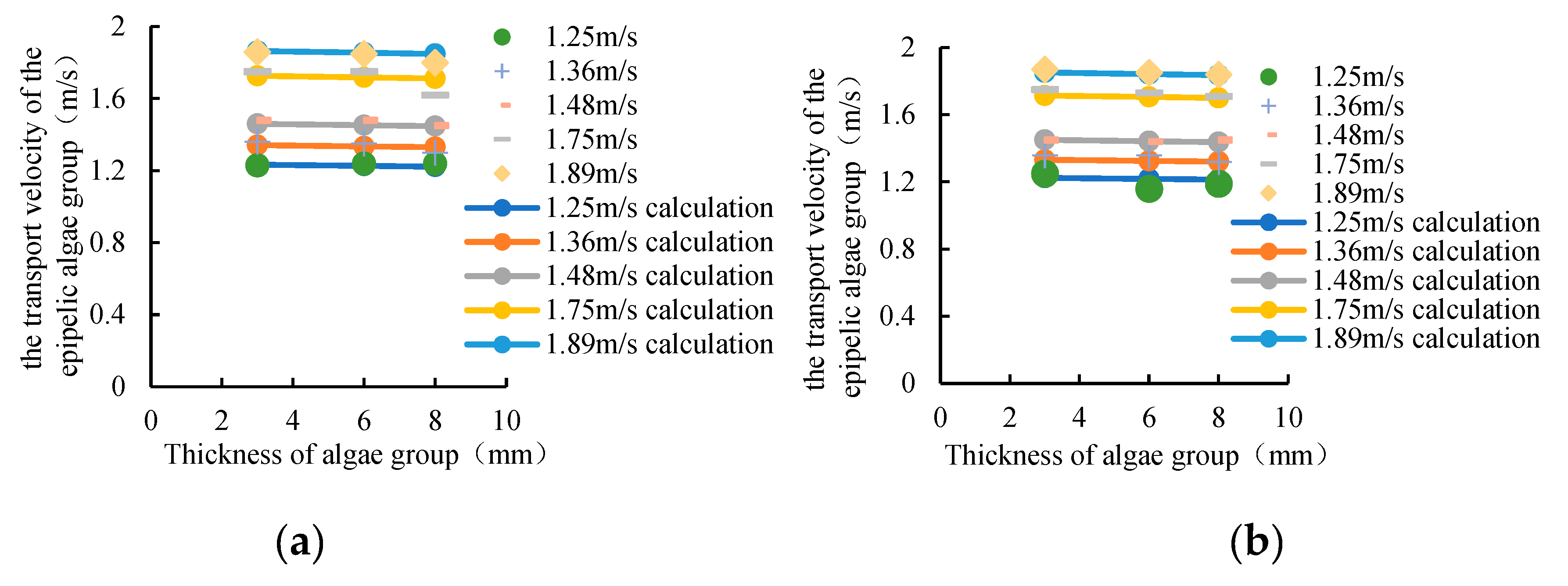
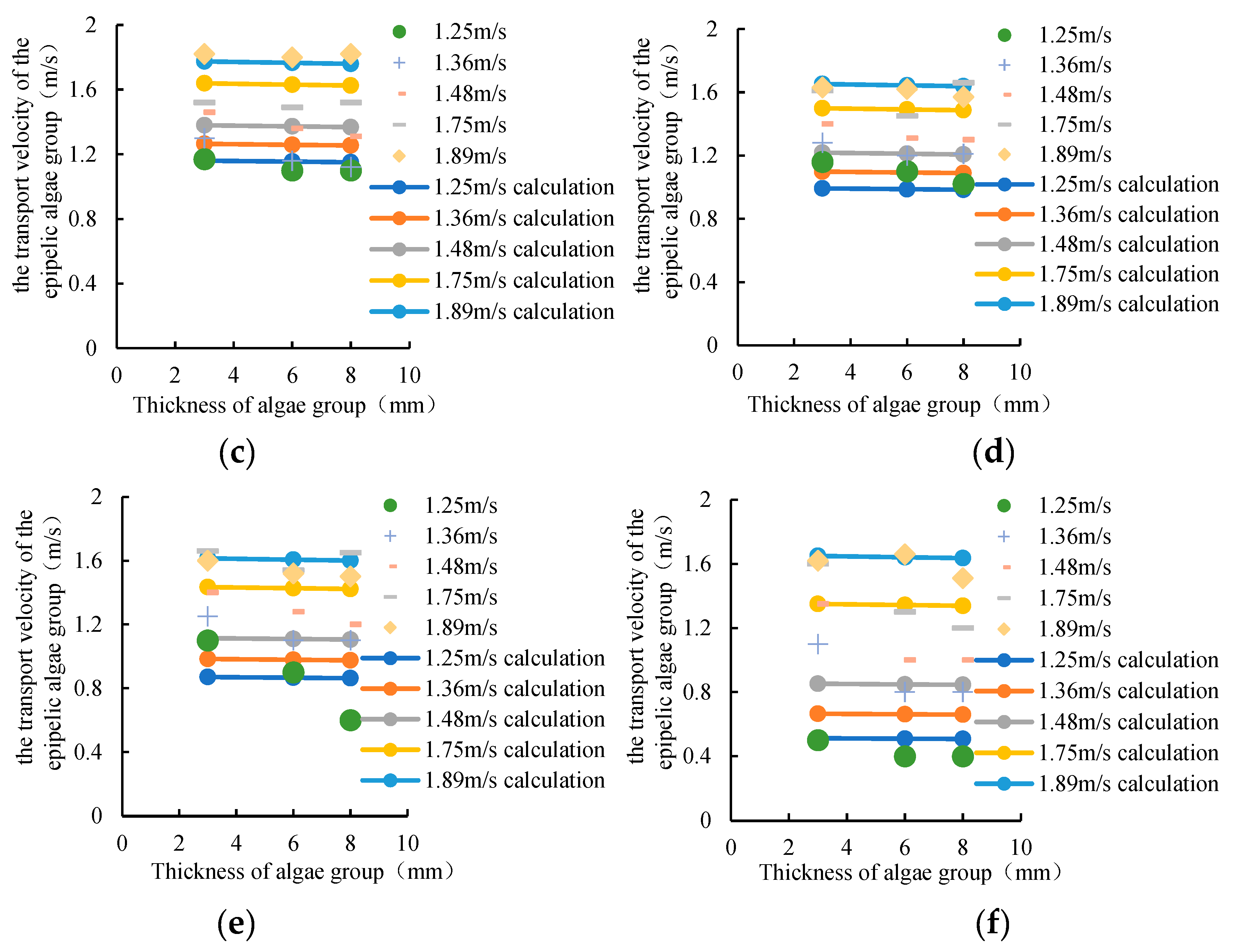
Figure 9.
Transportation of different areas of of epipelic algae groups: (a) the thickness of epipelic algae groups is 3mm; (b) the thickness of epipelic algae groups is 6mm; (c) the thickness of epipelic algae groups is 8mm.
Figure 9.
Transportation of different areas of of epipelic algae groups: (a) the thickness of epipelic algae groups is 3mm; (b) the thickness of epipelic algae groups is 6mm; (c) the thickness of epipelic algae groups is 8mm.
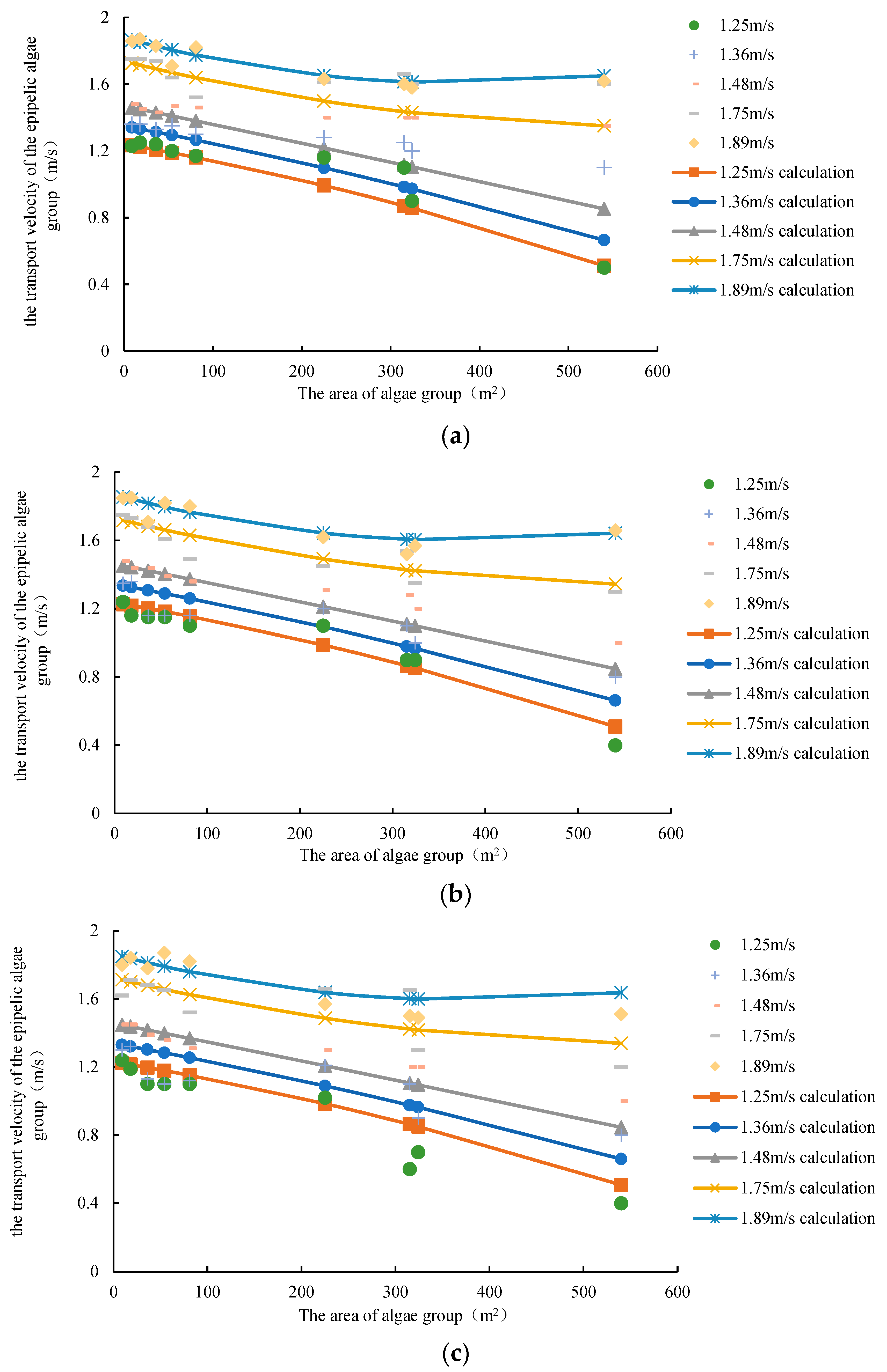

Table 1.
The percentage of the transport velocity of the epipelic algae group to the mainstream velocity.
Table 1.
The percentage of the transport velocity of the epipelic algae group to the mainstream velocity.
| Flow rate (m3/s) | 36.53 | 68.03 | 102.04 | 220.84 | 301.69 | |
| the mainstream velocity (m/s) | 1.25 | 1.36 | 1.48 | 1.75 | 1.89 | |
| Length×Width of algae group | Thickness of algae group | The percentage of the transport velocity of the epipelic algae group to the mainstream velocity (%) | ||||
| 3m×3m | 3mm | 98.25 | 99.89 | 100.00 | 100.00 | 98.24 |
| 6mm | 99.44 | 99.39 | 100.02 | 100.00 | 98.13 | |
| 8mm | 99.51 | 96.01 | 97.97 | 92.42 | 95.12 | |
| 6m×3m | 3mm | 100.35 | 100.12 | 97.82 | 100.10 | 98.94 |
| 6mm | 92.97 | 100.12 | 97.13 | 98.73 | 97.80 | |
| 8mm | 95.05 | 97.18 | 97.97 | 97.71 | 97.36 | |
| 6m×6m | 3mm | 99.20 | 97.63 | 96.54 | 99.26 | 96.71 |
| 6mm | 92.00 | 85.13 | 97.39 | 96.20 | 90.56 | |
| 8mm | 88.00 | 83.31 | 94.17 | 95.91 | 94.30 | |
| 9m×6m | 3mm | 96.00 | 99.39 | 99.32 | 93.80 | 90.66 |
| 6mm | 92.00 | 85.40 | 94.01 | 91.78 | 96.39 | |
| 8mm | 88.00 | 80.98 | 92.06 | 94.56 | 98.68 | |
| 9m×9m | 3mm | 93.60 | 95.70 | 98.86 | 86.94 | 96.28 |
| 6mm | 88.00 | 85.40 | 92.21 | 85.20 | 95.24 | |
| 8mm | 88.00 | 82.45 | 88.51 | 86.78 | 96.49 | |
| 15m×15m | 3mm | 92.80 | 94.23 | 94.59 | 92.24 | 86.51 |
| 6mm | 88.00 | 88.34 | 88.51 | 82.65 | 85.66 | |
| 8mm | 81.60 | 89.08 | 87.84 | 95.13 | 83.28 | |
| 21m×15m | 3mm | 88.00 | 92.02 | 94.59 | 94.75 | 84.66 |
| 6mm | 72.00 | 80.98 | 86.49 | 87.92 | 80.43 | |
| 8mm | 48.00 | 80.98 | 81.08 | 94.27 | 79.37 | |
| 18m×18m | 3mm | 72.00 | 88.34 | 94.59 | 91.43 | 83.60 |
| 6mm | 72.00 | 73.62 | 81.08 | 77.14 | 82.96 | |
| 8mm | 56.00 | 66.26 | 81.08 | 74.29 | 78.89 | |
| 30m×18m | 3mm | 40.00 | 80.98 | 91.22 | 91.43 | 85.82 |
| 6mm | 32.00 | 58.89 | 67.57 | 74.29 | 87.91 | |
| 8mm | 32.00 | 58.89 | 67.57 | 68.57 | 80.06 | |
Disclaimer/Publisher’s Note: The statements, opinions and data contained in all publications are solely those of the individual author(s) and contributor(s) and not of MDPI and/or the editor(s). MDPI and/or the editor(s) disclaim responsibility for any injury to people or property resulting from any ideas, methods, instructions or products referred to in the content. |
© 2024 by the authors. Licensee MDPI, Basel, Switzerland. This article is an open access article distributed under the terms and conditions of the Creative Commons Attribution (CC BY) license (http://creativecommons.org/licenses/by/4.0/).
Copyright: This open access article is published under a Creative Commons CC BY 4.0 license, which permit the free download, distribution, and reuse, provided that the author and preprint are cited in any reuse.


