Submitted:
08 March 2024
Posted:
11 March 2024
You are already at the latest version
Abstract
Anticipating and planning for the urgent response to large-scale disasters is critical to increase the probability of survival in these events. These incidents present various challenges that complicate the response, such as unfavorable weather conditions, difficulties in accessing affected areas, and the geographical spread of the victims. Furthermore, local socioeconomic factors such as insufficient prevention education, limited disaster assets, and inadequate coordination between public and private emergency services may complicate these situations. In large-scale emergencies, multiple hotspots are usually observed, which requires efforts to coordinate the strategic allocation of human and material resources in different geographical areas. Therefore, the precise management of these resources based on the specific needs of each area becomes fundamental. To address these complexities, this paper proposes a methodology that models these scenarios as an optimization problem, focusing on the location and allocation of resources in mass casualty incidents. The proposed case study is Mexico City in a post-earthquake scenario, using voluntary geographic information, open government data, and historical data from the September 19, 2017 earthquake. Additionally, it is assumed that the resources that require optimal location and allocation are ambulances, which focus on medical issues that affect the survival of victims. The designed solution involves the use of a metaheuristic optimization technique, along with a parameter tuning technique, to find configurations that perform at different instances of the problem, i.e., different hypothetical scenarios that can be used as a reference for future possible situations. Finally, the objective is to present the different solutions graphically, accompanied by relevant information to facilitate the decision-making process of the authorities responsible for the practical implementation of these solutions.
Keywords:
multiobjective optimization
; mass casualty incidents
; geographic information systems
MSC: 90C29
1. Introduction
The International Federation of Red Cross (IFRC) defines a disaster as “an event that disrupts the normal functioning conditions of a community and exceeds its ability to deal with the effects with its own resources [1]". The term natural risks refers to natural phenomena that have the potential to cause a disaster, such as climatologist, meteorologist, hydrologist, biological, or geophysical phenomena. Given the natural conditions of the planet, all geographic regions are exposed to different types of natural risks that have the potential to cause a disaster and are inevitable and sometimes unpredictable. However, disasters that could occur deriving from these are avoidable, and it is the responsibility of the population to prepare to reduce its impact in three different stages: before the event (proactive), during the event (active), and after the event (reactive). The World Health Organization (WHO) defines four phases for disaster management: prevention, to minimize the effects of the incident; preparation, to plan the actions to take in each dangerous situation and to educate the population on the subject; response, to act immediately after the incident and provide medical assistance and resources; and finally recovery, to return to normal once the tasks associated with the response phase are completed [2].
If a disaster leads to a high number of casualties beyond the capabilities of healthcare providers, it is considered a Mass Casualty Incident (MCI). The medical issues resulting from a Mass Casualty Incident (MCI) are defined by the National Association of Emergency Medical Technicians (NAEMT) in the Manual for Prehospital Trauma Life Support (PHTLS) [3] that include the following five elements:
- Search and rescue: This activity involves identifying and removing victims from a dangerous situation.
- Triage and initial stabilization: This is the process of classifying victims according to the severity of their injuries and the primary medical care they require.
- Patient monitoring: refers to continuously monitoring a patient’s health status from identification to evacuation.
- Definitive medical care: it is the component in which specialized care is provided to the patient according to his needs until his recovery is complete.
- Evacuation: refers to the transfer of the patient from the disaster area to the area of definitive medical care.
These elements describe the tasks carried out in the disaster response phase from a medical perspective, although there are other aspects to consider when participating in an MCI. One of the most widely used risk management tools is the Incident Command System (ICS)[3,4] which is designed to facilitate the coordination of agencies in different jurisdictions to work effectively together. This system is based on an organizational structure for managing the response to an incident, small or large. The ICS describes best practices for trained personnel to address the five medically relevant elements safely and efficiently; however, various factors can make the scenario more complex, such as the dynamic nature of a disaster, the uncertainty of the damage caused and the location of the victims, among others.
A scenario that can occur in large-scale disasters is when there is a large geographic area (fires, floods, earthquakes and pandemics), where there are multiple focal points and the victims are not concentrated in a single area, which means that personnel cannot move between them in a reasonable amount of time. In this scenario, the process to assign the available resources needs to be analyzed. The ICS recommends that "to avoid the problems that might be caused by the massive convergence of resources to the scene and to manage them effectively, the Incident Commander (IC) may establish the required holding areas".
In these types of situations, “units are typically sent to a staging area rather than going directly to the incident location" [3]. A staging area, or preparation area, is a location near the incident where multiple units can be held in reserve, and dinamically assigned as required. With this in mind, a hypothetical ambulance allocation proposal is to allocate only those ambulances necessary to care for confirmed victims at each care center, then place the rest of the available ambulances in one (or more) staging areas, and then allocate them to nearby care centers as the presence of victims is confirmed.
This assignment means that an ambulance will go to a focus of attention, paramedics will evacuate the victim to a hospital, and return to the staging area, thus distributing the workload among all the available units. However, this requires the selection and activation of staging zones that ensure that:
- They are close to the centers of attention to which ambulances will be directed.
- The number of activated zones does not create an unnecessary logistical problem.
- They have easy access to the roads and do not represent an obstacle for vehicle traffic.
For this reason, it is recommended to identify the candidate staging areas in advance. From these candidates, the areas to be activated can be determined according to the disaster conditions. In the state-of-the-art, various authors consider hospitals and ambulance bases as starting points that can be used as stating areas. However, this approach is not applicable to all countries and cities considering the local characteristics of hospital and prehospital infrastructure. Alternatively, transportation infrastructure can be used to temporarily locate these types of resources, as long as it satisfies the previous requirements. In summary, there are three major tasks to solve this problem:
- Define a methodology to find candidate areas to reduce the search space, given the number of road segments that can be considered as staging areas.
- Find the best staging areas to activate from the set of candidate zones, taking into account the travel time to the attention centers and the number of activated zones.
- For each enabled staging area, assign the focus of attention to cover, considering proximity and capacity.
Currently, several approaches have been used to address resource location and allocation problems with specific constraints. Halper et al. [5] proposed a dynamic model using the Mobile Facility Location Problem (MFLP) to relocate existing facilities and allocate customers to minimize transportation and travel costs. The authors suggested using a Geographic Information System (GIS) to identify candidate locations and constrain the search space. In disaster situations, Saeidian et al. [6] compared a genetic algorithm with a bee algorithm to find the optimal location of help centers and allocate support resources. The authors suggested using a geographic information system (GIS) to identify candidate locations and constrain the search space.
In the context of ambulance placement and allocation, Wang et al. [7] addressed the identification of temporary bases and temporary medical centers with budget constraints. They proposed hybrid metaheuristics to assign ambulances to temporary stations and distribute them to affected areas. On the other hand, Kaveh et al. [8] used the Maximum Coverage Location Problem (MCLP) approach for ambulance location and assignment and proposed an Improved Biogeography-Based Optimization (IBBO) algorithm. The authors designed a four-dimensional migration model consisting of primary, secondary, elite, and random habitats to improve local search and random search algorithms. To evaluate the performance of the proposal, they were compared with a genetic algorithm and with the Particle Colony Optimization algorithm. Geographic Information Systems and Analytical Hierarchical Process (AHP) were used to select candidate sites and constrain the search space.
Taking these aspects into account, there is an opportunity to improve the ability to respond to disasters by optimizing the use of medical assistance resources, reducing the impact they can have on the number of human losses. In the present work, these three tasks are addressed in a specific study area, adapting to local protocols and regulations; however, the methodology developed and the mathematical model of the problem can be adapted to other regions, as long as relevant information is available.
2. Materials and Methods
The proposed methodology is shown in Figure 1 and consists of seven stages: Problem Model, Historical Data, Incident Data, Data Integration, Algorithm Selection, Optimization Process, and Solution Visualization. The purpose of each stage and its components are described in the following.
2.1. Problem Model
The problem can be described as a combination of the p median problem and the maximum coverage problem, with two objectives: the first is to minimize the cost (distance) between the temporary bases of activated ambulances and their respective assigned demand points (see Equation 1), and the second is to activate the smallest possible number of temporal bases (see Equation 2). Taking into account the observation in [9] on the problem of p-median, it is established that if you have a solution with p installations, increasing another installation in any of the candidate nodes that do not have an installation will reduce the total weighted cost. Therefore, the objective function will decrease. However, in the proposed model, adding an installation p deteriorates the second objective, so there is a conflict between the two objectives. The problem model is defined by
- is the i-th ambulance time base (decision variable).
- is the i-th demand point.
- I is the set of candidate bases.
- J is the set of demand points.
- U is the set of urgencies of the demand points.
- is the coverage from to (decision variable).
- C is the cost matrix of .
- is the cost to go from to .
- is the capacity of .
- is the demand for .
- is the urgency of .
- is the maximum cost that a route can have.
Here, the two objective functions are:
Several definitions of the p-median problem specify that . However, this is not always possible when the problem has limited capacity. For this reason, a criterion must be defined to process each , taking into account demand , capacity , distance , or urgency (examples of the calculation of urgency can be consulted in [10]). The methods for processing each j-th element are as follows:
- Classic: A is randomly chosen and assigned to the nearest .
- Urgency-based: is calculated and processed in descending order of .
- Based on demand and urgency: It is ordered based on and later on .
2.2. Historical Data
It consists of acquiring or generating the information from the case study on which the problem is analyzed. Examples of information needed include transportation infrastructure, hospital locations, reception centers, temporary refuges, and potential staging areas. Some of this data was obtained from open-access databases and official sources. The remaining data set is generated specifically for the problem.
Official data. These data were obtained from the Mexico City Open Data Portal (Portal de Datos Abiertos de la Ciudad de México, in Spanish) and the Risk Atlas Portal (Atlas de Riesgos, in Spanish). All layers were modified to homogenize the common features and were reprojected to SRS EPSG:6369, Mexico ITRF2008/ UTM Zone 14N. The names of the layers and each attribute are written in lowercase, and a crop was applied using the bounding polygon of Mexico City.
Transport network. A graph is generated using the OSMNX Python library using the Mexico City polygon as a reference. A multi-digraph object is obtained from NetworkX, where the edges represent the roads and the vertices describe their intersections. All components of the graph are georeferenced with the SRS EPSG:4326, so a reprojection is applied to the system EPSG:6369.
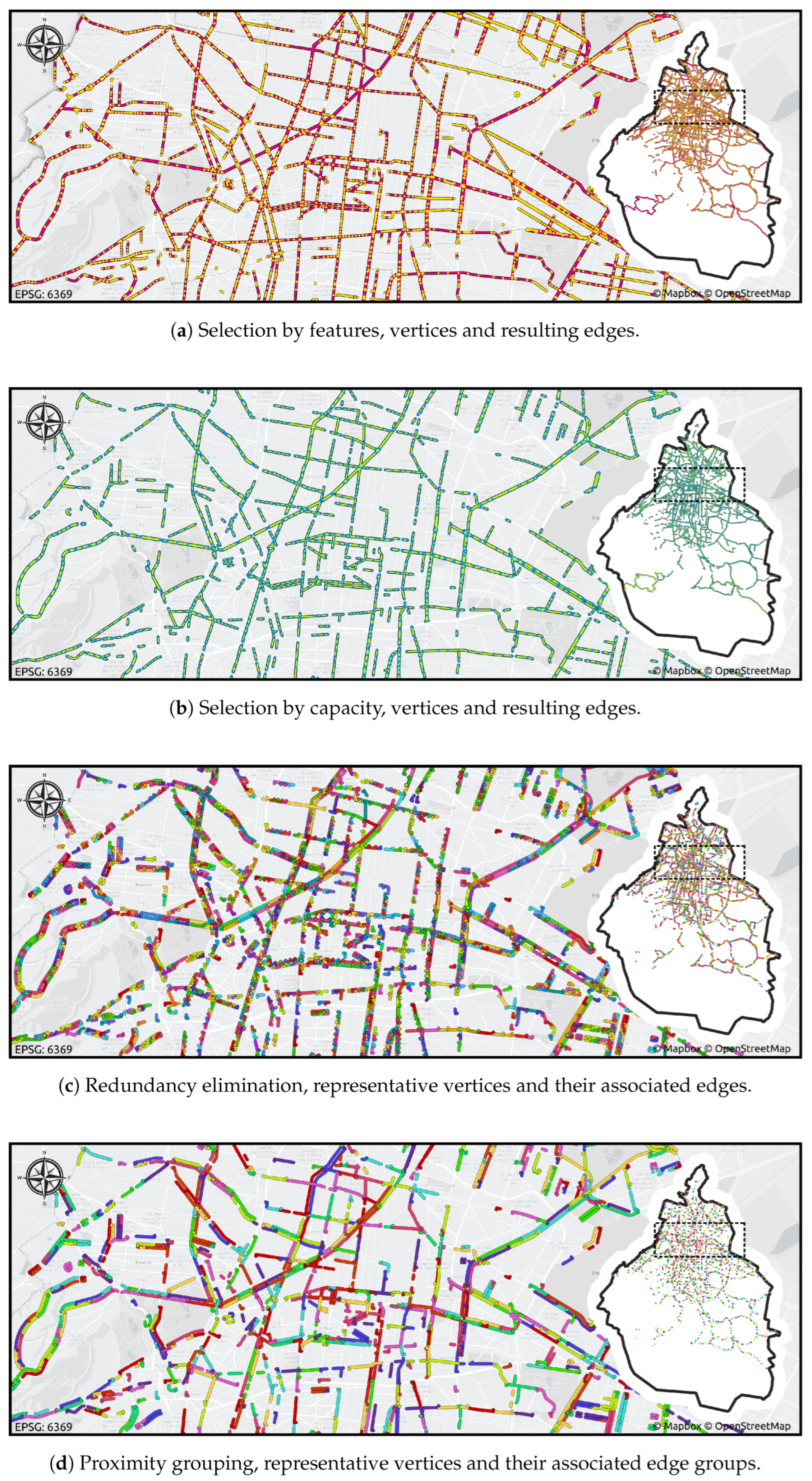
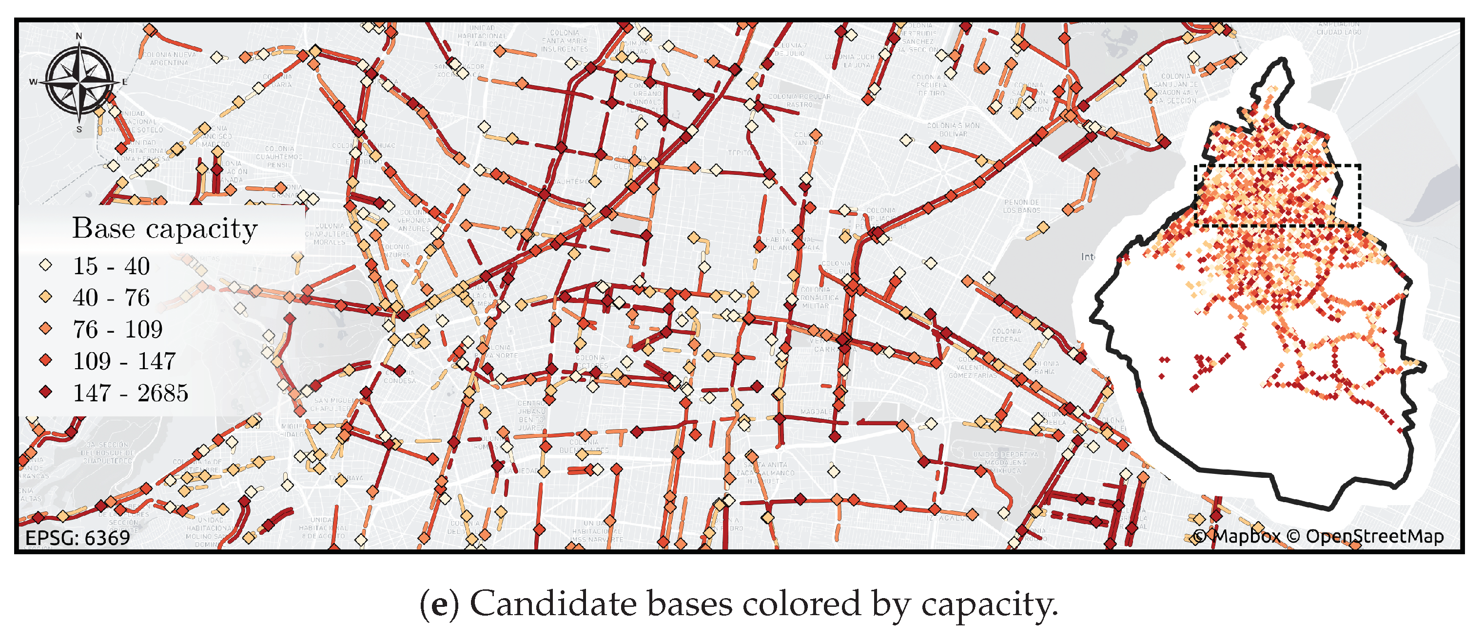
Candidate bases. Several approaches assume that the candidate locations where the ambulances will be placed are known a priori and are typically hospitals. In Mexico City, there is no official data, but in practice, the same transportation infrastructure is usually used to place ambulances. Applying this alternative in other models, each road could be considered as a candidate location, i.e. there would be 305,190 possible locations using the roads individually, or 128,825 taking only the intersections as starting points. However, the search space for the location problem would be , which is not computationally efficient. Therefore, in this work, a methodology based on [11] is proposed to segment the transportation network, described as a transportation graph , and to obtain a filtered graph , such that , considering a limit representing the minimum capacity () as well as a proximity factor (). The methodology used is described below.
-
Selection by characteristics: Roads with any of the following characteristics are discarded:
- It is a highway, incorporation, residential street, or it has no classification.
- They have less than 3 lanes.
- It is represented with a bidirectional edge and has less than 4 lanes.
- The number of lanes is unknown and has a lower hierarchy than the type of secondary road.
- Selection by capacity: Roads are discarded, where it is not possible to assign a minimum of ambulances. On average, the length of an ambulance is considered equal to 6 meters and with . Furthermore, isolated vertices are eliminated and the filtered graph is updated with the capacity factor.
- Elimination of redundancy: Henceforth, roads are represented by their terminal vertex, i.e. the vertex v of the road , because this is the point from which an ambulance will start, and at intersections two or more roads can have a common terminal node. To avoid redundancy, roads that share a terminal node v are grouped, but their individual characteristics are preserved. As a result, a subset of vertices is obtained, which stores the attributes of the edges , and contains two new attributes: the length and the total capacity, which are the sum of the lengths and capacities of the grouped edges, respectively.
- Proximity grouping: The vertices of the set that are “close” are grouped according to a proximity parameter . This proximity factor is measured by the path from point to point using a path in . Using a clustering algorithm, information from multiple vertices is added to a representative vertex v.
Finally, a simplification process is applied, in which the edges representing connected roads without intersections are merged, i.e. the edges are merged into if the vertex v has no neighbors (either ancestors or predecessors) except u and w. For this reason, edges in the graph representation represent more than one road, having multiple attribute values such as name, type, number of lanes, etc. In the previous methodology, these merged roads are considered as a single road of the type of lower hierarchy present in the merged roads, i.e. if a primary road and a secondary road have been merged, the new edge is considered as a secondary road, but preserves the original attributes of the merged roads. To verify the coverage that the bases have throughout the city, the distance between each vertex of and its nearest base is evaluated using the Voronoi diagram of the graph with the resulting candidate bases as control points, i.e. the set V. To detect possible changes in this coverage, different weights can be applied to the edges using historical traffic data.
2.3. Incident Data
In this stage, event information is collected from the location of the centers of attention, considering the confirmed or possible number of victims, as well as blocked roads, traffic data and available hospital capacity. In a real scenario, these data are obtained from government sources as the information is being integrated. In an experimental scenario, historical data from previous incidents are used.
Location of attention focuses. The CDMX open data portal provides georeferenced data on buildings that collapsed or suffered damage during the September 19, 2017 earthquake, which can be used to estimate the probability distribution of damage locations that could occur in future events. It is proposed to generate new hypothetical scenarios that follow this spatial distribution and enable an adjustment of the algorithm parameters based on different instances of the same problem, using the density kernel of the buildings damaged in the 2017 earthquake, using the library scikit learn and a Gaussian kernel. To determine the kernel bandwidth, a grid search is performed (in one dimension) with 1000 values of powers of 10, from to . For each bandwidth value, the KDE is obtained using the leave one out validation method, and the maximum cumulative log-likelihood (max log-likelihood) is selected.
In addition, the demand for each of them has to be estimated. In a real scenario, the responsible official reports the location of the incident and its characteristics to make an initial estimate of the damage per quadrant [12]. This estimate includes details of damaged buildings (does not change), as well as the number of victims (may change as more specific information becomes available). The official data reported in the September 2017 earthquake do not have this information; therefore, it is proposed to make an approximation of the number of victims by using the points generated with the density kernel, the data from the land census and the SEDUVI, which requires the following modifications:
- Only residential buildings with information on the number of levels are considered.
- If a building does not have the number of levels but the height, then half of the height in meters is used as the number of levels.
- For blocks that do not have the average number of occupants, the average of the surrounding blocks is used.
To estimate the number of victims in each , the following steps were performed:
- n points are sampled using the kernel with :
- Search for the nearest building in the land records layer using Euclidean distance.
- The block in which each building is located is identified by calculating the Euclidean distance between the building and the centroids of the blocks.
- The average number of occupants per apartment in the block is taken and rounded to the closest integer using the ceiling function.
- If the building has three floors or less, it is considered a single-family unit, so the number of victims of the block is equal to .
- If the building has more than three levels, it is considered a multifamily building, and the average number of residents in the block is multiplied by the number of levels .
Traffic data. Traffic data can be obtained in real time through TomTom’s TrafficFlow API according to the specifications provided on the website, which is in raster format and segmented into rectangular tiles of fixed size, representing an exponential division of space [13]. To optimize the memory required to maintain all tiles, the data is converted to single-band rasters that preserve the different traffic classes by mapping the RGB components with a range of to a class index of .
When tiles are available as single-band raster data, a sampling is performed for each edge of the graph. This is done by calculating the center of the sampling window, which is the end of the line segment perpendicular to the intermediate line segment of the edge geometry and crossing its center. The final result of the traffic data extraction is a Pandas dataframe that associates the id of each edge with an integer value for each color that corresponds to the most frequently used value in the sampling window. However, if the sample window does not contain a number other than 0, it is assumed to represent free traffic and assigned the number 1.
At this stage, the Previous Data and Incident Data are concentrated and processed. Analysis is performed to ensure that all geographic data is in the same coordinate system and that all files are properly formatted. The incident data updates the status of previous data, such as the possibility of traveling along the road axes, obtaining a geospatial model that describes the complete scenario of the incident. Specifically, this stage consists of the following processes:
Upload Information. The data previously obtained must be loaded, processing the following information:
- Candidate locations as temporary bases I, . Since bases are a subset , they are identified by the id of the vertex in , i.e., the node attribute is used as an index.
- The transport graph .
- The location of hospitals with more than 10 beds.
- The points where the victims are located are identified by an denoted num.
- Traffic data associated with the incident.
Update previous data with incident data. For each particular scenario, the following data must be modified before running an optimization technique, in order to consider the specific characteristics of each incident:
- The traffic information is included in the traffic graph as an attribute traffic of the edges. If historical traffic data is used, all available data collected on the same day of the week with the nearest time to the event is obtained.
- A version of the graph is obtained in which there are no vertices that cannot be reached from a candidate base. Since the download of excludes unclassified roads, some points cannot be traveled from a temporary base. This does not mean that they cannot be accessed, but only that they will not be considered as a destination point, and the nearest available edge or vertex will be considered instead. To determine which points must be discarded, the Voronoi diagram of is calculated using the candidate bases as control points. The vertices that are not grouped in any cell are eliminated from G, resulting in a graph .
- The nearest edge to each demand point and to each hospital in the graph is identified. These edges are stored with their identifier in independent lists that will be used later.
- The edges of that are not traversable are identified, either because they have a value of 5 or 6 in the traffic classification, or if it is the nearest edge to and is found in the list of edges from the previous step. All edges of are assigned a state attribute locked and marked true for those identified in this step.
-
The edge costs of are calculated as the weight attribute as follows:
-
If the value of the block attribute is false, the value corresponding to the mapping traffic→weight is assigned as the value of the weight attribute:
- -
 1
1
- -
 2 .
2 .- -
 3 .
3 .- -
 4
4
Where l is the length of the edge and the coefficient is the inverse of the speed, expressed as distance. - On the other hand, if the lock attribute is true, the maximum weight is .
-
-
Candidate bases that satisfy any of the following conditions will be identified:
- It has no successors in the graph (this can occur at the boundaries of the zone).
- Some of the grouped edges are found in one of the lists in step 3, i.e., there is a demand point or a hospital in one of the streets it represents.
- They have a traffic value greater than 2.
These bases are discarded for use in the optimization problem, so they are not included in the calculation of the cost matrix. - The graph is updated with the new edge attributes.
Computation of the cost matrix. The resulting set I is used to calculate the origin-destination matrix (matrix C). To define the targets (set J), we take the two endpoints of the nearest edge to each focus and use the vertex with the highest cost to consider the worst-case scenario. If the most expensive vertex to reach requires traveling through the blocked path, the lowest-cost point is considered. The result is the set J, where each element represents the closest vertex of the graph to the true location of each focus of attention with the estimated number of casualties.
Assuming , it is more efficient to compute and run Dijkstra’s algorithm times than to use and run the algorithm times. The result is the cost of traveling from each vertex of to , which is stored in a Pandas dataframe that relates the id of each vertex and its distance to j. In addition, another dataframe is stored that relates each vertex to its predecessor. Finally, the dataframes define the cost matrix, where each row represents a base and each column represents a demand point . The relationship between position (row or column number) and base identifier (node attribute) or the demand point (num attribute) is stored to know which indices i and j correspond to each base and demand point, respectively. The implementation of Dijkstra’s algorithm is based on the Cugraph library.
Demand estimate. At this stage, the constants are estimated. Given that each has limited capacity, at this stage, the constants are estimated. Since each has limited capacity and the total number of ambulances must be distributed to cover the total demand, the demand for each is estimated with the ratio between the number of victims at that point and the total number of victims. After identifying the closest activated bases, the number of ambulances assigned to each group can be adjusted, provided that there is a tolerance in the total capacity of each base. To have a tolerance in the capacity of each base, half of the total capacity is taken as a value. Equation 11 describes the calculation of the demand for a point.
Where is the number of victims in and k is the number of ambulances available to satisfy the total demand. There are varying data on the number of ambulances available in Mexico City, although most of the sources consulted agree that there are more than 290 ambulances. Considering that not all of them will be available at the time of a disaster, it is proposed to use the number of 250 ambulances.
Instance Storage. When all the data used to describe the problem are available, the data is stored as Python objects. This process is performed for each of the 10 hypothetical scenarios proposed. Each scenario has its own focus location and random data from one week in November at different times.
2.4. Algorithm Selection
The NSGA-II Genetic Algorithm was used and to improve the performance of the algorithm, its parameters were modified with the following procedure:
Design and Implementation. The implementation of the NSGA-II algorithm is carried out using the Python library . The algorithm works with solutions using a feasible first selection method, as described in the [14] library documentation. To solve the optimization problem, several objects are defined below.
Problem and solution representation. This is an object that describes the mathematical model of the problem. Algorithm.It is the object through which the proposed algorithm is carried out. It receives as input the parameters of the algorithm and three additional parameters:
- Remove duplicates: A Boolean parameter that indicates whether or not solutions that are the same in the current population should be removed. There is no guarantee that there will be no repetition of solutions from previous generations that have been removed. In this paper, this value is set to true (True).
-
Stop criteria: It is an object that contains the criteria that determine when the algorithm stops, which remain fixed for all configurations with the values:
- xtol: Tolerance in the decision space.
- ftol: Tolerance in the target space.
- period: Criteria evaluation period.
- n_skip: Ignore generations for criteria evaluation.
- n_max_gen: Maximum number of generations.
- n_max_evals: Maximum number of evaluations of items.
Tolerance values are used to compare the Pareto fronts of the current generation and a generation from a previous period , each n_skip generations. This comparison depends on the space in which it is done. That is,- In the decision space (xtol), two Pareto fronts and are compared using the equation:where y
- In the target space (ftol), the inverse generation distance is calculated between the normalized fronts to be compared, that is: .
-
Repair function: Depending on the assignment method, the different solution vectors b can change and be reduced to the same solution vector, because activated bases that do not correspond to any demand point are discarded. There are two ways to repair:
- Normal repair: The assignment process is performed and the modified solution vector b that satisfies the required constraints is returned for the algorithm to perform duplicate removal in the current population.
- Repair with mutation: The assignment process is performed and the modified solution vector b is checked; If this vector has already been obtained after the assignment process, regardless of the number of generations, the solution vector is mutated and the assignment process is performed iteratively until a valid modified vector that has not been evaluated before is obtained, that is, an unexplored solution.
Since the assignment process is performed during repair and then before evaluation (for new solutions), it is important that the assignment is the same at both times, i.e., the same b always produces the same a. In the case of the urgency and on-demand methods, this is not a problem, since they are deterministic methods; but in the case of the classical method, the first assignment must be recorded for posterity, since it has a stochastic component. For this purpose, a dictionary is used for storing the pairs (b,a), where b is encoded with the hash method sha256.
Parameter selection. Since each algorithm requires a specific set of parameters, the correspondence between the required parameters and the information described in the geospatial model, whether categorical or numerical variables, is determined. Categorical variables can be different methods of performing an internal procedure of the algorithm, such as the assignment process, crossover and mutation operators, and the metric used to measure performance, among others. Numerical variables are the hyperparameters of an algorithm that can take different integer or real values, such as the number of individuals, the percentage of crossover and mutation, and the number of offspring, among others. For numerical variables, it is important to define a finite set of options to limit the search space. The Table 1 shows the parameters among which it is proposed to find a configuration that can solve the problem in a reasonable time. The values that categorical-type parameters can take are the following:
- un: Cross uniform.
- hun: Cross half uniform.
- bf: Bit flip mutation (bitflip).
- bfo: Active Bit Flip Mutation (bitflip on).
- cl: Classic allocation method.
- ur: Urgency allocation method.
- urc: Allocation method by demand and urgencies.
- rn: Normal repair.
- rm: Repair with mutation.
The biased bit flip mutation operator uses a probability of for active bits (value 1) and zero for inactive bits (value 0). In addition, for each inverted bit, another bit is inverted that is different from all the bits that were originally inverted, so that the number of active bits remains intact after the mutation. Note that the probability of mutation refers to the probability of a chromosome mutating, and each bit within the chromosome has a fixed probability of mutation of . Similarly, the probability of crossover represents the probability that two chromosomes will recombine, and each bit has a probability of inheriting children of 0.5.
Furthermore, the parameter is kept fixed for all instances and the ideal value of meters is proposed, that is, 9 minutes of response from the candidate base to the point of care, assuming one travels at a constant speed of . The value of 9 minutes is a standard recommended by [16] and used in the [17] and [18] models. However, this is an ideal case, so they also propose a range between 9 minutes. This proposal assumes that there is at least one ambulance on standby at each focus, which is assigned the moment a victim is confirmed, and another unit is immediately requested from the corresponding base, even if there is no other confirmed victim. Thus, a response time in that range would be required only in the worst case.
Setting parameters The parameter tuning technique irace was used through its official library in R. Since this technique is designed for single-objective algorithms, it must be adapted to a multi-objective problem by representing the Pareto front by a scalar value [15]. There are several ways to scalarize the Pareto front. Some require knowledge of the ideal Pareto front to quantify their similarity. Since no ideal front is known, these alternatives are not an option. On the other hand, in the implementation guide irace [15] suggests the use of the hipervolumen indicator, which requires a reference point to scalarize a Pareto front that can be used as a comparison metric between different algorithms or configurations.
The reference point for this metric should be chosen to ensure that every solution on the Pareto front contributes to the hypervolume. For this reason, it must be greater than the maximum value of each objective. To guarantee this, the point is defined as the reference point and both objectives are normalized from 0 to 1 by dividing the value of each by the maximum possible value, i.e:
where P is the Pareto front obtained by the algorithm, and the maximum for each objective O is calculated using Equations 14 and 15:
Regarding the implementation of irace, the parameter files are defined together with the scenario and target-runner.py, which is the program that provides the interface between R and the program that receives the parameters and executes the algorithm. In the scenario, a budget of is defined, and the execution method is: “execute_threaded_timeout” with a maximum of two execution attempts per configuration and a maximum time of 420 seconds (7 minutes), after which the execution of irace aborts. To avoid interrupting the execution in the target-runner, a maximum time of 6 minutes is defined for the internal execution of the algorithm. This is based on the assumption that a reasonable time to obtain a solution is 5 minutes plus the time it may take to load the data or generate the instance data. This means that the target-runner time limit is always reached, because the optimizer itself stops the execution when the 6 minutes limit is exceeded and returns a value. If it completes in time, it returns the value of the inverse of the hypervolume of the Pareto front obtained, and if it exceeds the time, it saves the configuration parameters and returns a value of 1 to indicate poor performance and discard it. Note that irace is a minimization algorithm by default, so the inverse of the hypervolume is considered as the evaluation metric.
Performance evaluation. It enables evaluation of the result of different configurations in different cases of the problem. The result is a set of elite configurations. Their performance can be compared to determine how to implement them in future problems. For this purpose, the five elite configurations with the best performance are taken as a reference, along with the three instances that describe the lowest, median and highest number of demand points. To observe the convergence to the Pareto front of the elite configurations, the algorithm is executed 20 times with different random seeds for each elite configuration, obtaining the minimum, maximum, average and standard deviation value of the hypervolume indicator to compare with the information obtained in the parameter adjustment stage. According to the performance of the configurations and the requirements in case of an emergency, different paths are chosen to find the solutions to present, for example, to the decision manager:
- Run the algorithm with the best performance multiple times using different random seeds, until the maximum time is reached.
- Run the algorithm with the different elite configurations obtained as many times as possible without exceeding the maximum time.
For this purpose, the time required for the execution of the algorithm, as a function of its parameters, must be recorded, weighting the importance of the quality of the solution and the speed with which it is generated. Additionally, the execution times of the last 20 iterations per configuration are recorded. To make comparisons between configurations, the median value (50th percentile) of the inverse of the hypervolume is used as a reference, which represents the maximum value that 50% of the executions will have.
2.5. Optimization Process
This stage performs the algorithm using the parameters with the best performance obtained in previous stages. For new cases, steps 1, 2, 3, 4, and 6 should be executed using the algorithm with the best combination of parameters. After the result is obtained, the decision maker must choose one of the available options on the Pareto front to decide how the temporary bases are allocated. By performing multiple executions, the multiple Pareto fronts obtained are merged, and the non-dominated solutions separated, among which the final decision for subsequent implementation will be made. To avoid the fact that multiple executions do not represent a disadvantage in terms of sequential execution time, parallelization of the executions is proposed using the joblib library. In the process of determinng final solutions, if there are activated bases that cover a single point, the actual assignment of ambulances will be made directly to the waiting area of that point, instead of using the closest temporary base determined by the algorithm, since it is not relevant to assign ambulances to a neighboring base.
2.6. Solution Visualization
Once the Pareto front with the candidate solutions is computed, it is possible to plot it to facilitate decision making. For this purpose, the following elements will be displayed on a map of Mexico City:
- The location of the attention centers, showing the number of resources required.
- The location of the activated bases, displaying the number of ambulances.
- The routes from each enabled base to each assigned focus of attention. They are identified by using a different color for each base and their cost.
- Boundaries of townships.
- The attention regions defined in the earthquake emergency plan serve as a reference to assign a person directly responsible for the administration of each base, depending on where they are located.
- The location of the hospitals and, if available, the number of beds available.
- The location of collection centers and refuges.
Visualization is performed using the geopandas library, which contains functions that allow other functions of the folium library to be implemented indirectly, providing visualization parameters without having to develop an implementation from scratch. The product of using this library for visualization is a .html file that can be included in a web page for visualization.
2.7. Implementation Plan
Once the decision maker selects a solution, the implementation plan must be defined to coordinate response activities with different emergency services. Although this stage is not part of the objectives of this research, a proposal is presented to relate the solution to the current earthquake action plan. Initially, more information is obtained from the selected solution, as follows:
- Voronoi diagram with activated bases: The Voronoi diagram of the graph can be obtained using activated bases as control points. In the case of the external Voronoi diagram, the routes for each vertex of the graph are obtained as the destination and the closest activated base as the origin, which can be useful for addressing other incidents that occurred after the current solution was chosen. In the case of the internal Voronoi diagram, the route can be obtained from any vertex of the graph to its closest activated base, allowing one to identify the shortest route that ambulances can take to the assigned base from any point they encounter.
- Voronoi Diagram with Hospitals: By obtaining the internal Voronoi diagram of using the vertices closest to each hospital as control points, we obtain the shortest path from any other vertex in to the nearest hospital. This can be useful in determining which hospital to take patients depending on the location of the victims, whether it is an isolated victim being transported in a private vehicle or a victim from a care center being transported in an ambulance.
-
Attention Flow: Once the available ambulances have been assigned to the activated bases as preparation points, a person in charge of each is designated and the commander in charge of the attention centers is notified that they will be served by that base. The sequence they must follow to distribute the workload is as follows:
- -
- At least one ambulance must remain in the waiting area near the attention center.
- -
- Once a victim is confirmed, he is assigned to the ambulance in the staging area and the appropriate staging area is notified to dispatch another unit.
- -
- The victim is transported to the nearest hospital and the ambulance returns to the same staging area from which it originated, taking the last spot in line. On the way back to the staging area, you can choose to load fuel.
- -
- If one of the bases runs out of ambulances and still has demand, ambulances from other bases with lower demand can be arbitrarily reassigned, omitting the formula for estimating demand and adapting the solution to the new emergency conditions.
- Changes in the Emergency Situation: Although a static model is considered at the time the optimization algorithm is performed, some actions are required to adjust the solution to the new conditions. First, when a significant number of headlights are introduced, the algorithm is repeated, reassigning the ambulances from the old solution to the closest bases from the new solution. If the changes are primarily traffic-related, and there is an Internet connection, it is possible to perform the traffic query to generate the new weights of the edges with these data, and then compute the routes from the bases to the ambulances. However, since the bases are already activated, instead of performing the entire optimization process from scratch, it is sufficient to obtain the external Voronoi diagram with the bases as control points to find the new paths. In this case, the Voronoi algorithm would update the assignment vector a based on the previous solution vector b, but it cannot ensure that the constraints defined in the model are satisfied.
3. Results
The computing equipment used to implement the methodology has an Intel Core i9-9900K processor and NVidia GeForce RTX 2080 graphics card; consequently, all execution time measurements of the procedures are relative to these characteristics.
3.1. Data Generated: Candidate Locations
In order to solve the proposed problem, a first data set must be generated that describes the candidate locations that can be used as temporary ambulance bases. Table 2 describes the number of resulting elements after each step described in the preceding section. On the other hand, the steps to obtain the candidate locations in a specific area are sketched in Figure 2.
Figure 2.
Process for obtaining candidate bases.
To perform coverage analysis, we applied the weights corresponding to the average traffic at each edge according to the defined hours, considering traffic speeds of and . Applying the Voronoi diagram algorithm, the data in Table 3 were obtained. This table presents the percentage of graph vertices that are less than 9 minutes and the response time at which of the vertices are located ( percentile). This table reveals that the difference between the coverage at different times does not vary substantially. In particular, at 7 and 8 p.m. and 3 p.m., the percentage of vertices covered by the nearest base is smaller for the speed 20 . Note that higher speeds increase the percentage of vertices that can be reached from a candidate base in less than 9 minutes. Starting at , all vertices satisfy this property, which is essential to justify the maximum cost constraint used in the problem model.
3.2. Data Generated: Points of Attention
The density kernel used to generate the hypothetical scenarios is shown in Figure 3, where the best bandwidth value found () was used. The projection of the kernel on the X (longitude) and Y (latitude) axes is also observed with the projection of the original data used to generate the kernel (black lines).
In total, 10 hypothetical problem scenarios were generated, each associated with a random date and time from which traffic data can be obtained to define a problem instance. Figure 4 shows the scenarios with the lowest and highest number of points. To generate an instance of the problem, each hypothetical scenario is associated with a time and date from which traffic data can be obtained. The characteristics of these instances are described in Table 4.
3.3. Data Obtained: City Traffic
To capture traffic information for most of the streets in the CDMX by applying the procedure described in the methodology the following parameters and values were used:
- Zoom level: 16.
- Total number of tiles (to cover the bounding box): .
- Tiles occupied (intersecting the polygon of the CDMX): .
- Meters per tile: .
- Meters per pixel: .
3.4. Parameter adjustment
Once the instance generation process is finished, execution of irace is carried out with the implementation of the NSGA-II algorithm. The execution of the algorithm is characterized by the following features:
- Number of iterations: 10.
- Performed experiments: 4,982.
- Remaining budget: 18.
- Number of elites: 5.
- Number of settings used: 679.
- Total user time on CPU: 880930.4, (10.19 days).
The five elite configurations that performed the best on average are listed in order of performance in Table 5. There are parameter values that are repeated in most cases, including the uniform crossover operator (4/5), the emergency assignment method (5/5), the repair with mutation (5/5), the population of 200 with 50% offspring (5/5), the crossover percentage of 0.5 (4/5) and the mutation percentage of 0.5 (4/5). The experiments performed are shown in Figure 7, obtained using the Python code provided in [19]. This figure depicts that in the first iterations, parameters are sampled that generate regular configurations that do not converge near the minimum value found (marked with ); on the other hand, as the iterations advance, the elite configurations begin to appears in the graph (,), and most of the time they are found at the values closest to the known minimum. Furthermore, instances that were interrupted for exceeding the execution time of 6 minutes (they return 1 as a value) are shown at the top, and these instances were registered in a non-feasible configuration file. A total of 164 iterations were interrupted.
3.5. Solution Visualization
The result of the optimization process is a preview visualization, see Figure 9, of all the Pareto front solutions, described in Figure 8, and a table with the relevant data for each solution, see Table 6. Figure 10 shows the html file generated when processing solution number 8 (the knee point of the Pareto front). It is possible to interact with this generated map to visualize more information about the elements found.
4. Conclusions and Future Work
Relevant data can be obtained from official data sources in the study area to solve the problem of location and allocation of ambulances in scenarios with mass casualties in multiple focal points, from historical data on disaster incidents, to the location of complementary resources to the problem, such as hospitals, temporary shelters, collection centers, and the geographical delimitation of regions of care that designate the authorities responsible for the provision of emergency services.
The proposed methodology to find candidate emergency response areas (temporary bases) allows finding a subset of representative vertices in the graph modeling the transportation network, from which at least of the remaining vertices are expected to reach within 9 minutes of 40 km/h, considering different times of day. In contrast to the alternative of using the complete transportation network in the problem model, the resulting search space contains only of the locations. Although the identification of candidate bases is carried out statically, it is possible to discard more bases by considering complementary event data, such as traffic data.
By obtaining the set of roads that can be used as temporary ambulance bases with their respective capacities, the location of the focal points with their respective estimated number of victims, and the graph that models the transportation network, it is possible to model the problem of ambulance location and allocation as a dual objective optimization problem. This model requires the identification of the bases to be activated (location) and the focal point served by each one (allocation), subject to eight constraints that ensure the congruence of the solution and limit the solutions to viable regions, considering the maximum response time or the maximum number of bases to be activated.
From the kernel density estimate of the historical data of the buildings damaged by the earthquake of September 19, 2017, it is possible to generate hypothetical scenarios of the problem. For each scenario (hypothetical or real), a specific instance of the same problem was generated. To generate such an instance, the read time of the data and the procedure have approximately the same duration, but the time needed to compute the cost matrix is proportional to the number of demand points.
The Dijkstra algorithm was used to obtain the cost matrix by inverting the graph and running it twice for each demand point, using as the origin the end points of the edge that is closest to the demand points. Implementing this algorithm using graphs from the Cugraph library accelerated this calculation by approximately 300
The ER allocation method was considered one of the best configurations compared to the classical method and the demand-based method, suggesting that the relationship between base capacity and point of care demand in this problem is not significant enough to benefit from a method that considers the demand first and the proximity afterwards.
The possible parameter values included populations of small size (20, 50) and a percentage of descendants. On the other hand, the mutation repair method outperformed the normal repair method, indicating that the procedure used to discard already explored solutions tends to improve the performance of the algorithm. A more rigorous analysis is needed to verify the relationship between these parameters and the algorithm performance, but these results provide a baseline for designing the required experiments.
The evaluation of the elite configurations on three representative instances with 20 random seeds suggests that although these configurations stand out from other regular configurations evaluated in parameter tuning, better techniques and configurations still need to be evaluated to obtain more accurate results with less variability, exploring solutions on the Pareto front with a smaller number of activated bases; however, the quality of the solutions is improved by merging the Pareto fronts of multiple runs of the same configuration, with the disadvantage of requiring more time. However, by parallelizing the multiple runs to generate the unified Pareto front, the result was obtained in half the time of a sequential execution.
The different solutions of the Pareto front suggest different ways of assigning the ambulances to the focus locations, and the previsualizations allow intuitive identification of which points remain isolated and which bases should be activated. The final visualization, generated in .html format, can be used for further implementation in a context that allows the emergency medical services involved in the care plan to visualize the information interactively, to show or hide elements of interest depending on the circumstances.
Author Contributions
Conceptualization, M.S.-P. and G.G.; methodology, M.M.-P. and M.S.-P.; software, V.K.L.-S. and G.G.; validation, G.G. and M.S.-P.; formal analysis, M.M.-P. and V.K.L.-S; investigation, M.M.-P. and V.K.L.-S; resources, V.K.L.-S. and M.S.-P.; data curation, G.G. and M.M.-P.; writing—original draft preparation, V.K.L.-S. and M.M.-P.; writing—review and editing, G.G. and M.M.-P.; visualization, M.M.-P. and G.G.; supervision, G.G. and M.M.-P.; project administration, M.S.-P. and G.G.; funding acquisition, M.S.-P. and G.G. All authors have read and agreed to the published version of the manuscript.
Funding
This work was partially sponsored by the Instituto Politécnico Nacional under grants 20240426, 20240632, the Consejo Nacional de Humanidades, Ciencias y Tecnologías.
Acknowledgments
We are thankful to the reviewers for their time and invaluable and constructive feedback, which helped improve the quality of the paper.
Conflicts of Interest
The authors declare no conflicts of interest.
References
- The International Federation of Red Cross and Red Crescent Societies. What is a disaster? Available online: https://www.ifrc.org/what-disaster (accessed on 4 November 2022).
- World Health Organization. Emergency cycle. Available online: https://www.who.int/europe/emergencies/emergency-cycle (accessed on 4 November 2022).
- American college of surgeons committee on trauma and Campos, Víctor and Roig, Félix Garcia. PHTLS Soporte Vital de Trauma Preshospitalario; Jones & Bartlett Learning, 2020.
- International Resources Group and "Oficina de los Estados Unidos de Asistencia para Desastres en el Extranjero para Latino América y el Caribe". Curso Básico Sistema de Comando de Incidentes; 2021.
- Halper, R.; Raghavan, S.; Sahin, M. Local search heuristics for the mobile facility location problem. Computers & Operations Research 2015, 62, 210–223. [CrossRef]
- Saeidian, B.; Mesgari, M.S.; Ghodousi, M. Evaluation and comparison of Genetic Algorithm and Bees Algorithm for location–allocation of earthquake relief centers. International Journal of Disaster Risk Reduction 2016, 15, 94–107. [CrossRef]
- Wang, J.; Wang, Y.; Yu, M. A multi-period ambulance location and allocation problem in the disaster. Journal of Combinatorial Optimization 2020, 43, 909–932. [CrossRef]
- Kaveh, M.; Mesgari, M.S. Improved biogeography-based optimization using migration process adjustment: An approach for location-allocation of ambulances. Computers & Industrial Engineering 2019, 135, 800–813. [CrossRef]
- Daskin, M.S.; Maass, K.L., The p-Median Problem. In Location Science; Springer International Publishing: "Cham, 2015; pp. 21–45. [CrossRef]
- Ghoseiri, K.; Ghannadpour, S.F. Solving capacitated p-median problem using genetic algorithm. 2007 IEEE International Conference on Industrial Engineering and Engineering Management. IEEE, 2007. [CrossRef]
- Medina-Perez, M.; Legaria-Santiago, V.K.; Guzmán, G.; Saldana-Perez, M. Search Space Reduction in Road Networks for the Ambulance Location and Allocation Optimization Problems: A Real Case Study. Telematics and Computing; Mata-Rivera, M.F.; Zagal-Flores, R.; Barria-Huidobro, C., Eds.; Springer Nature Switzerland: Cham, 2023; pp. 157–175.
- Secretaria de Gestión Integral de Riesgos y Protección Civil de la Ciudad de México and Urzúa, Myriam. Protocolo del Plan de Emergencia Sísmica; Gaceta oficial de la Ciudad de México, 2021.
- TomTom Developers. Zoom Levels and Tile Grid, 2023. Available online: https://developer.tomtom.com/map-display-api/documentation/zoom-levels-and-tile-grid (accessed on 9 September 2023).
- pymoo: Multi-objective Optimization in Python. Available online: https://www.pymoo.org (accessed on 02 September 2023).
- López-Ibáñez, M.; Dubois-Lacoste, J.; Pérez Cáceres, L.; Birattari, M.; Stützle, T. The irace Package: User Guide, 2022. Available online: https://cran.r-project.org/web/packages/irace/vignettes/irace-package.pdf (accessed on 21 October 2023).
- Fitch, J. Response times: myths, measurement & management. JEMS: a journal of emergency medical services 2005, 30, 46 – 56. [CrossRef]
- Zaffar, M.A.; Rajagopalan, H.K.; Saydam, C.; Mayorga, M.; Sharer, E. Coverage, survivability or response time: A comparative study of performance statistics used in ambulance location models via simulation–optimization. Operations Research for Health Care 2016, 11, 1–12. [CrossRef]
- Wu, C.; Hwang, K.P. Using a Discrete-event Simulation to Balance Ambulance Availability and Demand in Static Deployment Systems. Academic Emergency Medicine 2009, 16, 1359–1366. [CrossRef]
- de Souza, M.; Ritt, M.; López-Ibáñez, M.; Cáceres, L.P. ACVIZ: A Tool for the Visual Analysis of the Configuration of Algorithms with irace. Operations Research Perspectives 2021, 8, 100–186. [CrossRef]
Figure 1.
Proposed Methodology.
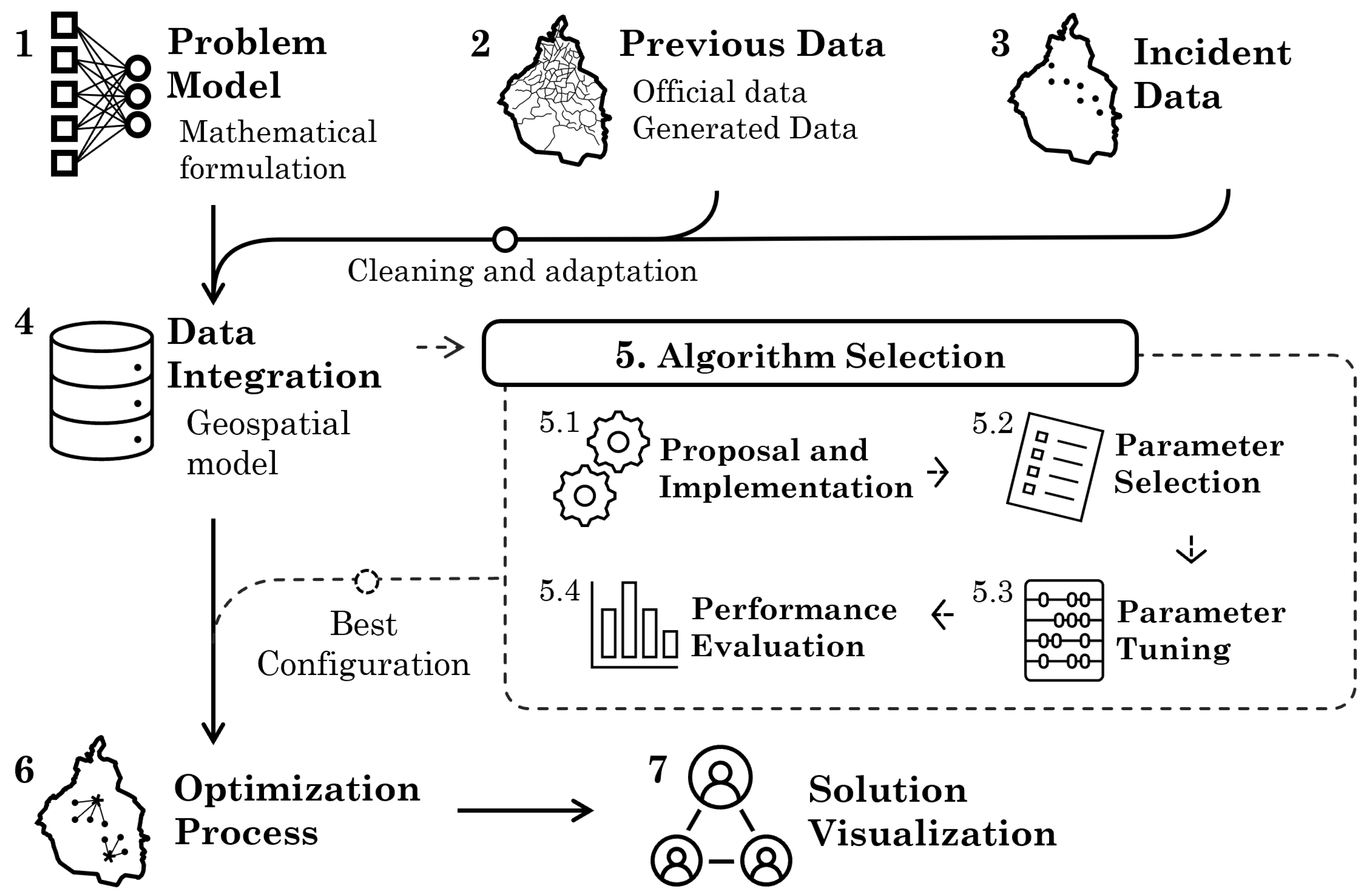
Figure 3.
Kernel Density Estimation of Buildings Damaged by the 09/19/2017 Earthquake.
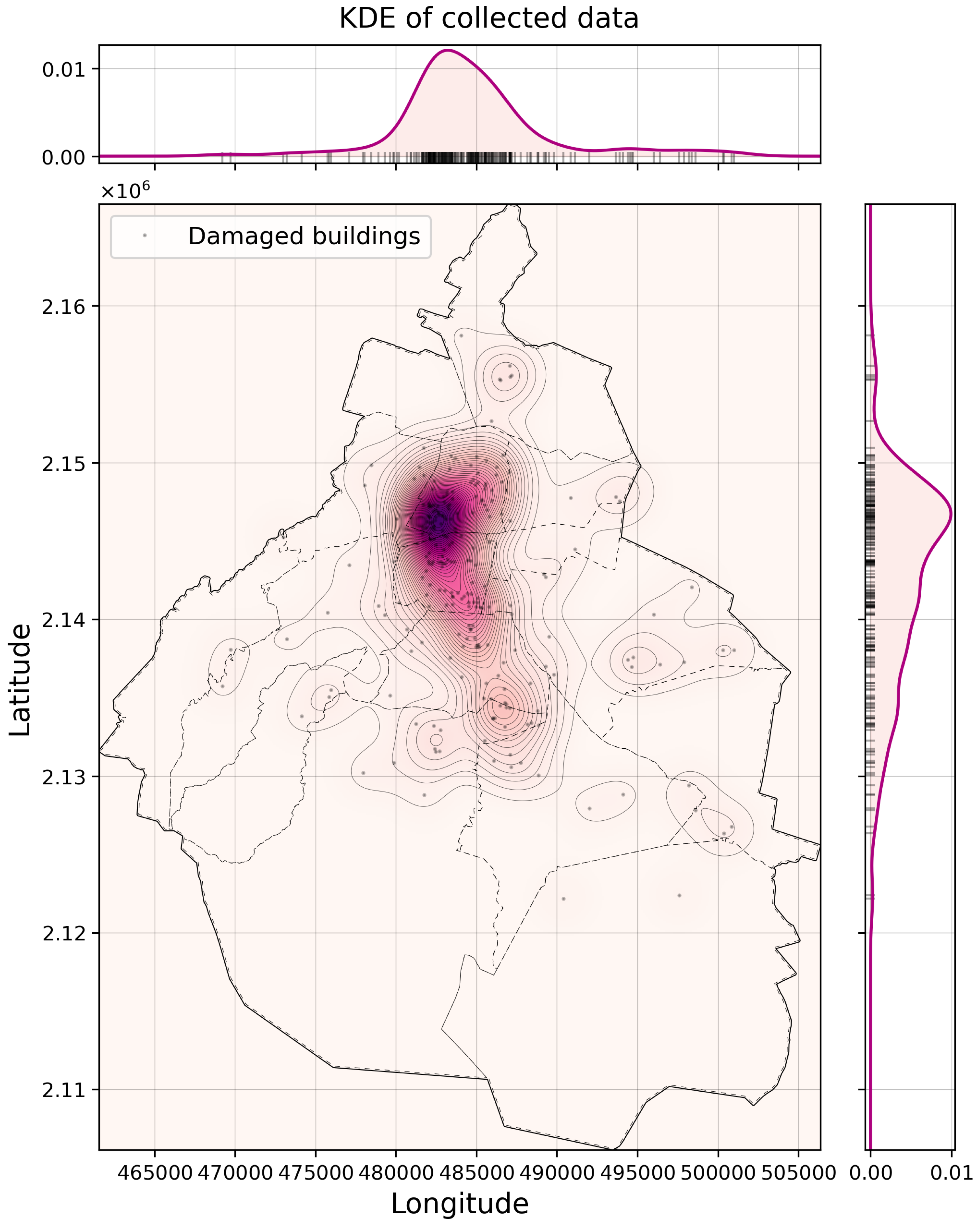
Figure 4.
Instances with the lowest and highest number of points described in Figure 3.
Figure 4.
Instances with the lowest and highest number of points described in Figure 3.
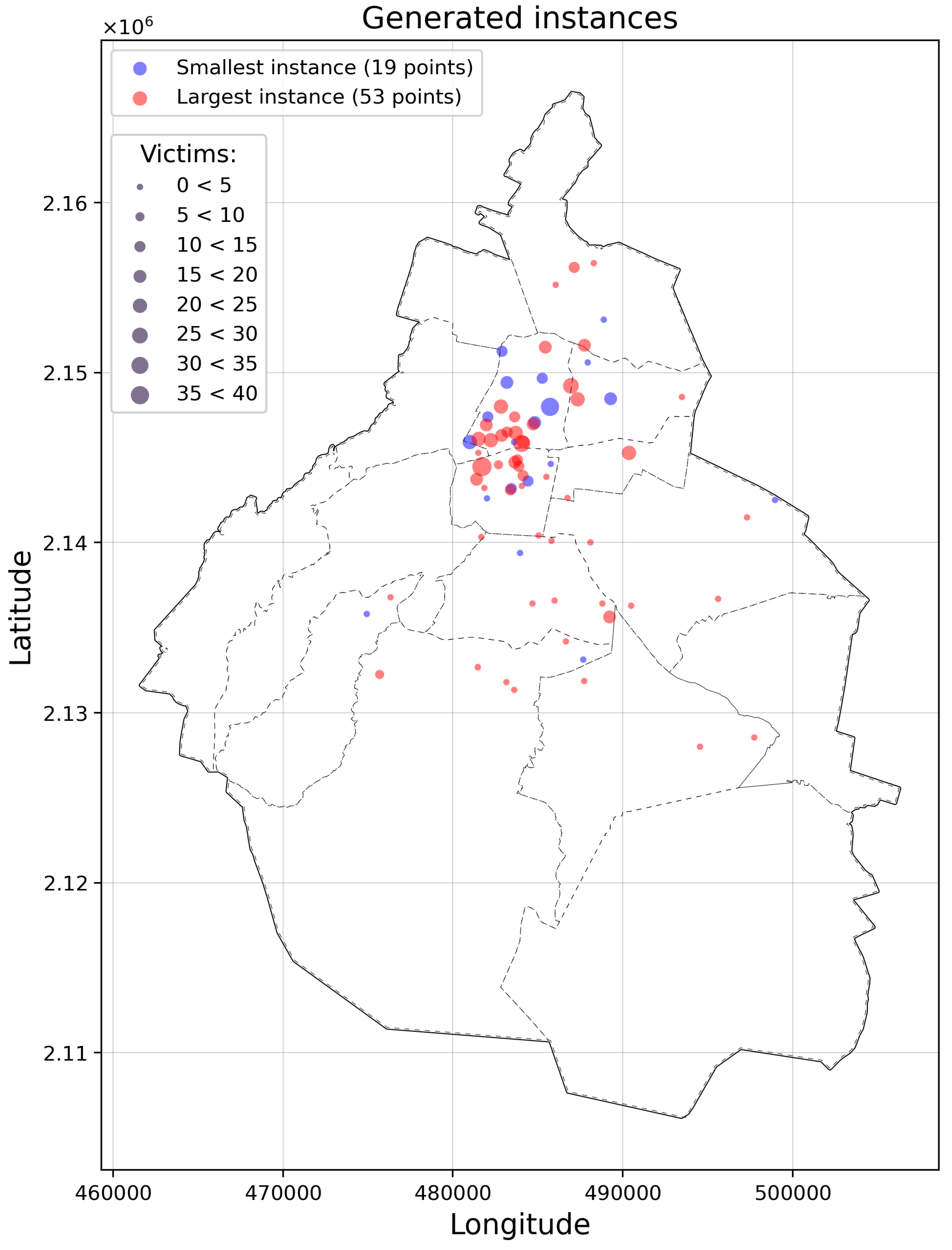
Figure 5.
Tiles used to determine the amount of traffic in Mexico City. Example of data obtained on November 14, 2023 at 13:45 hours.
Figure 5.
Tiles used to determine the amount of traffic in Mexico City. Example of data obtained on November 14, 2023 at 13:45 hours.
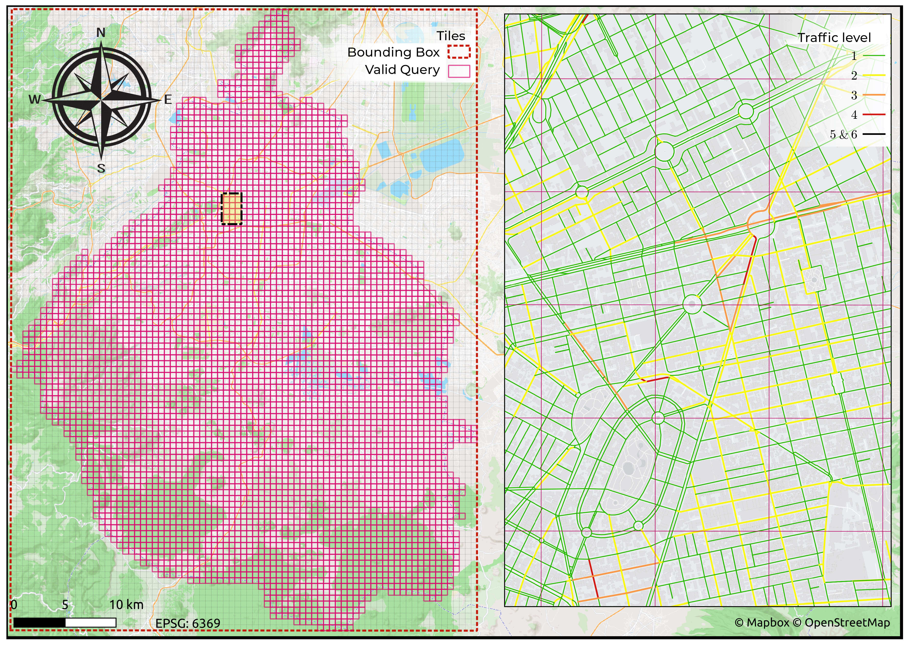
Figure 6.
Stages of obtaining traffic data in the OSMNX network.
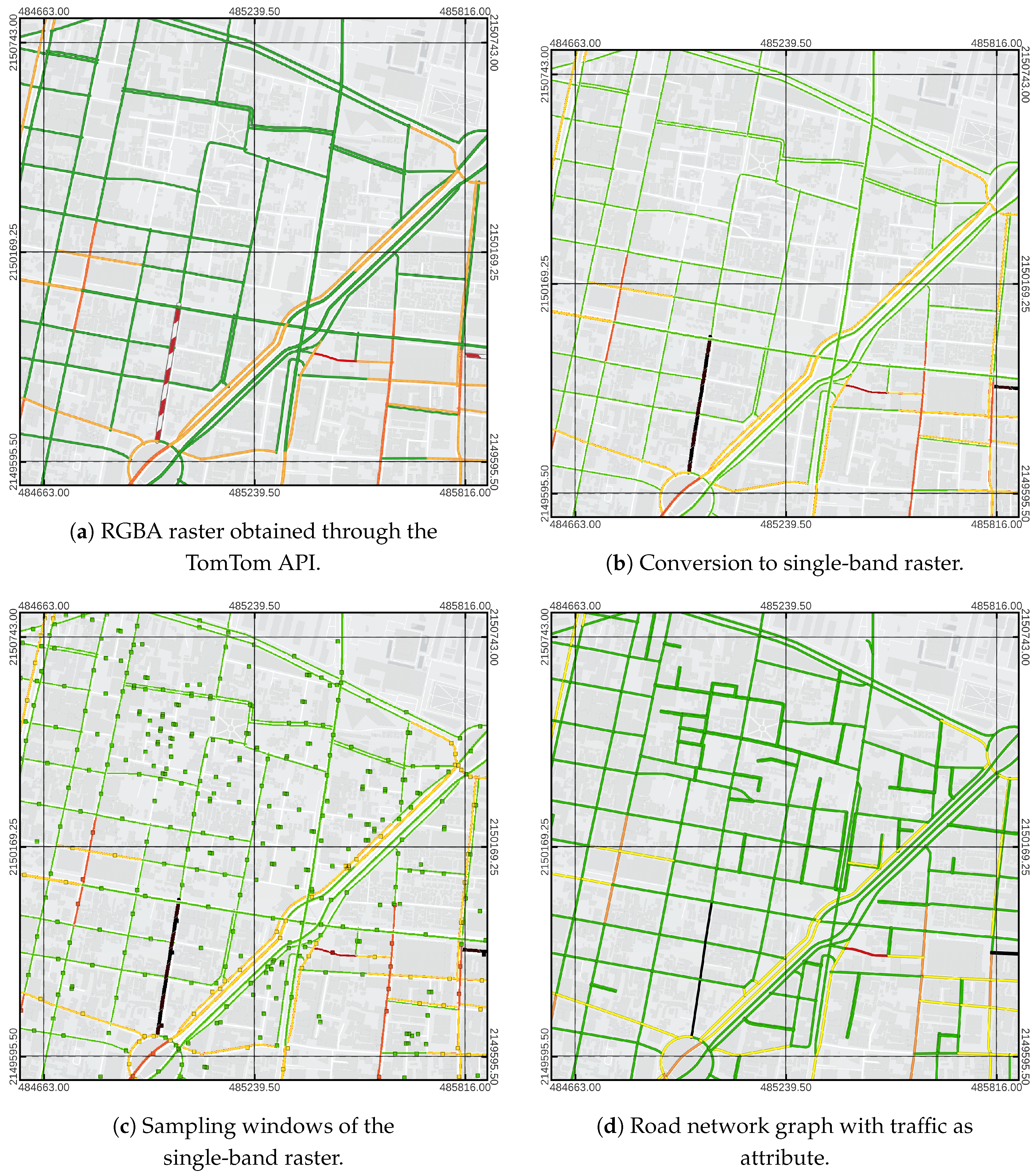
Figure 7.
Experiments performed during parameter tuning.
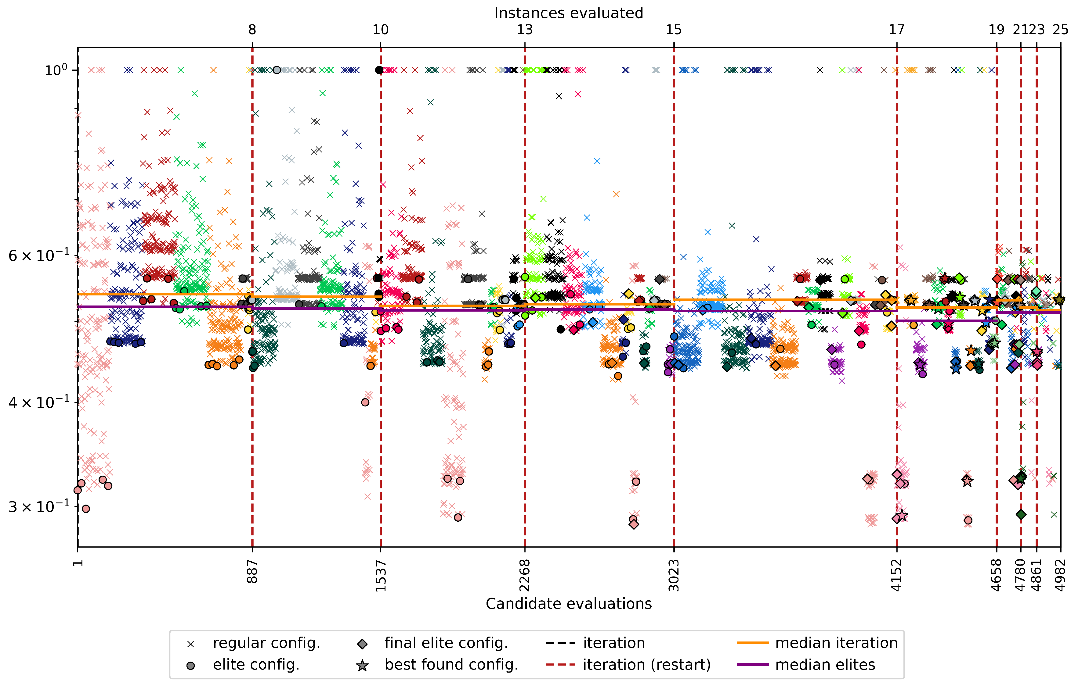
Figure 8.
Pareto front of the post-disaster scenario of the 2017 earthquake.
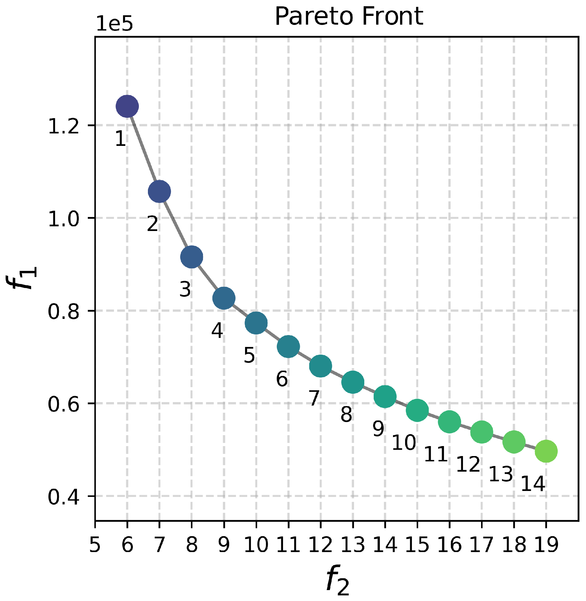
Figure 9.
Preview of the solutions 1, 8 and 14 for the 2017 scenario.
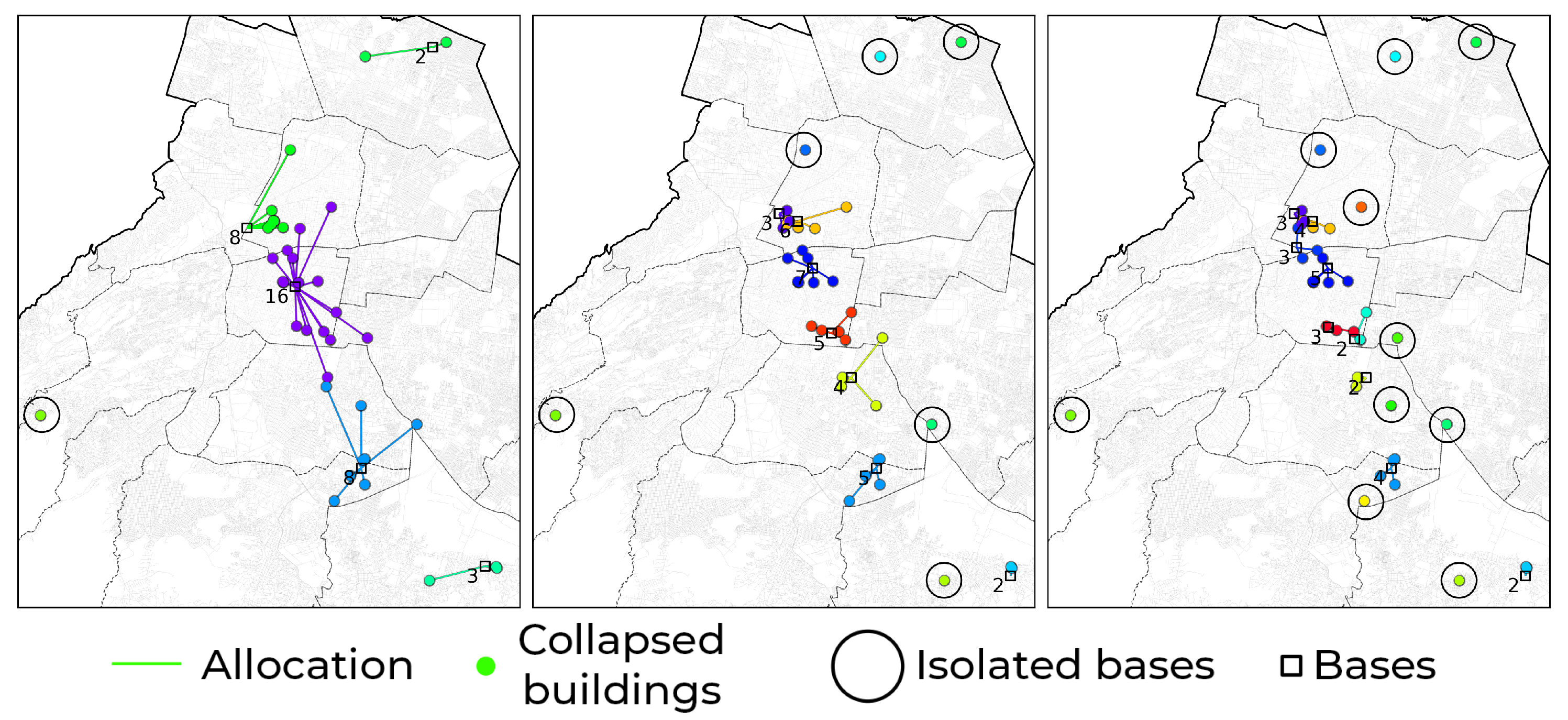
Figure 10.
Interactive visualization of the solution, displaying the available layers and the default map view.
Figure 10.
Interactive visualization of the solution, displaying the available layers and the default map view.
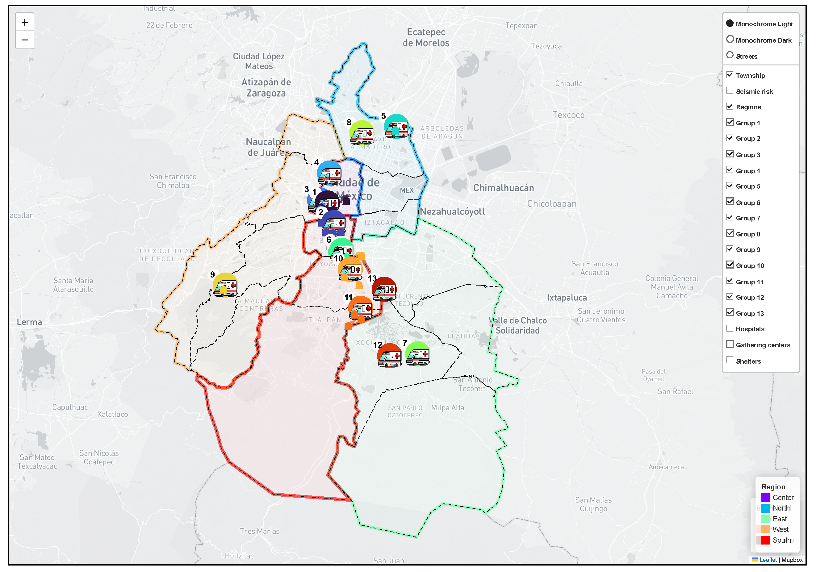

Table 1.
Possible values for algorithm parameters. c*= numeric attributes that are defined as categorical according to documentation [15].
Table 1.
Possible values for algorithm parameters. c*= numeric attributes that are defined as categorical according to documentation [15].
| Parameter | Name | Key | Type | Values |
|---|---|---|---|---|
| Crossover operator | crossover | –cr | c | (un, hun) |
| Mutation operator | mutation | –mu | c | (bf, bfo) |
| Allocation method | allocation | –a | c | (cl, ur, urc) |
| Repair method | repair | –rep | c | (rn, rm) |
| Population size | population | –pop | c* | (20, 50, 100, 200) |
| Percentage of offspring | offsprings | –dec | c* | (25, 50, 75) |
| Crossing percentage | prob_crossover | –prob_cr | c* | (0.5, 0.75, 0.9, 0.99) |
| Mutation percentage | prob_mutation | –prob_mu | c* | (0.5, 0.25, 0.1, 0.01) |
| Start probability | prob_initial | –prob_ini | c* | (0.25, 0.1, 0.01) |
Table 2.
Reducing transport network.
| Step | Result | Size |
|---|---|---|
| Transport network | ||
| Selection by characteristics | ||
| Selection by capacity | ||
| Elimination of redundancy | ||
| Proximity grouping | V |
Table 3.
Response time to vertices from the closest candidate base, %= percentage of vertices covered in less than 9 minutes, p95 = maximum response time for of vertices (95th percentile), =bases discarded by traffic .
Table 3.
Response time to vertices from the closest candidate base, %= percentage of vertices covered in less than 9 minutes, p95 = maximum response time for of vertices (95th percentile), =bases discarded by traffic .
| Daytime | 20 km/h | 30 km/h | 40 km/h | 50 km/h | 60 km/h | ||||||
|---|---|---|---|---|---|---|---|---|---|---|---|
| % | p95 | % | p95 | % | p95 | % | p95 | % | p95 | ||
| 7:00 am | 47 | 0.96 | 8.15 | 0.99 | 5.44 | 0.99 | 4.08 | 1.0 | 3.26 | 1.0 | 2.72 |
| 8:00 am | 69 | 0.96 | 8.25 | 0.99 | 5.5 | 0.99 | 4.13 | 1.0 | 3.3 | 1.0 | 2.75 |
| 9:00 am | 66 | 0.96 | 8.17 | 0.99 | 5.45 | 1.0 | 4.09 | 1.0 | 3.27 | 1.0 | 2.72 |
| 11:00 am | 52 | 0.96 | 8.09 | 0.99 | 5.39 | 1.0 | 4.04 | 1.0 | 3.24 | 1.0 | 2.7 |
| 1:00 pm | 74 | 0.96 | 8.39 | 0.99 | 5.59 | 1.0 | 4.19 | 1.0 | 3.36 | 1.0 | 2.8 |
| 3:00 pm | 122 | 0.95 | 8.75 | 0.99 | 5.84 | 0.99 | 4.38 | 1.0 | 3.5 | 1.0 | 2.92 |
| 5:00 pm | 57 | 0.96 | 8.47 | 0.99 | 5.65 | 0.99 | 4.23 | 1.0 | 3.39 | 1.0 | 2.82 |
| 7:00 pm | 139 | 0.95 | 9.0 | 0.98 | 6.0 | 0.99 | 4.5 | 1.0 | 3.6 | 1.0 | 3.0 |
| 8:00 pm | 55 | 0.95 | 8.71 | 0.99 | 5.81 | 0.99 | 4.36 | 1.0 | 3.49 | 1.0 | 2.9 |
| 9:00 pm | 21 | 0.96 | 8.45 | 0.99 | 5.64 | 0.99 | 4.23 | 1.0 | 3.38 | 1.0 | 2.82 |
Table 4.
General data of the instances that are created, : instance, X: discarded bases, : number of victims, d: demand
Table 4.
General data of the instances that are created, : instance, X: discarded bases, : number of victims, d: demand
| Date/hour | X | Total | min | max | mind | maxd | |||
|---|---|---|---|---|---|---|---|---|---|
| 0 | 27/10 - 09:00 am | 319 | 1527 | 43 | 334 | 2 | 45 | 2 | 26 |
| 1 | 27/10 - 03:00 pm | 482 | 1364 | 45 | 463 | 2 | 45 | 2 | 19 |
| 2 | 28/10 - 11:00 am | 265 | 1581 | 44 | 381 | 2 | 45 | 3 | 17 |
| 3 | 29/10 - 07:00 pm | 227 | 1619 | 38 | 515 | 2 | 45 | 2 | 67 |
| 4 | 30/10 - 1:00 pm | 240 | 1606 | 19 | 193 | 2 | 45 | 5 | 44 |
| 5 | 30/10 - 05:00 pm | 235 | 1611 | 53 | 570 | 2 | 45 | 2 | 16 |
| 6 | 31/10 - 07:00 am | 306 | 1540 | 23 | 192 | 2 | 45 | 5 | 29 |
| 7 | 01/11 - 08:00 am | 267 | 1579 | 37 | 275 | 2 | 45 | 3 | 16 |
| 8 | 01/11 - 08:00 pm | 280 | 1566 | 35 | 376 | 2 | 45 | 3 | 28 |
| 9 | 02/11 - 09:00 pm | 139 | 1707 | 26 | 302 | 2 | 45 | 2 | 34 |
Table 5.
Elite configurations.
| top | id | -cr | -mu | -a | -rep | -pop | -dec | -prob_cr | -prob_mu | -prob_ini |
|---|---|---|---|---|---|---|---|---|---|---|
| 1 | 625 | un | bf | ur | rm | 200 | 50 | 0.5 | 0.25 | 0.1 |
| 2 | 499 | un | bf | ur | rm | 200 | 50 | 0.75 | 0.5 | 0.25 |
| 3 | 432 | hun | bfo | ur | rm | 200 | 50 | 0.5 | 0.5 | 0.25 |
| 4 | 655 | un | bf | ur | rm | 200 | 50 | 0.5 | 0.5 | 0.1 |
| 5 | 617 | un | bfo | ur | rm | 200 | 50 | 0.5 | 0.5 | 0.1 |
Table 6.
Statistics of the Pareto front-end solutions of the 2017 scenario.
| Sol. | f1 | f2 | * | ||||
|---|---|---|---|---|---|---|---|
| 1 | 124065.2 | 6 | 7904.6 | 3264.9 | 1 | 2 | 16 |
| 2 | 105696.9 | 7 | 7800.3 | 2781.5 | 1 | 2 | 13 |
| 3 | 91577.8 | 8 | 6107.8 | 2409.9 | 1 | 2 | 8 |
| 4 | 82685.1 | 9 | 6258.1 | 2175.9 | 1 | 2 | 7 |
| 5 | 77329.4 | 10 | 6258.1 | 2035.0 | 2 | 2 | 7 |
| 6 | 72245.0 | 11 | 5013.1 | 1901.2 | 4 | 3 | 7 |
| 7 | 68039.6 | 12 | 4907.8 | 1790.5 | 5 | 3 | 7 |
| 8 | 64555.3 | 13 | 4907.8 | 1698.8 | 6 | 2 | 7 |
| 9 | 61456.4 | 14 | 4907.8 | 1617.3 | 7 | 2 | 7 |
| 10 | 58493.7 | 15 | 4907.8 | 1539.3 | 7 | 2 | 7 |
| 11 | 56013.6 | 16 | 4907.8 | 1474.0 | 8 | 2 | 7 |
| 12 | 53807.9 | 17 | 4907.8 | 1416.0 | 8 | 2 | 5 |
| 13 | 51680.9 | 18 | 4907.8 | 1360.0 | 9 | 2 | 5 |
| 14 | 49675.7 | 19 | 4907.8 | 1307.3 | 10 | 2 | 5 |
Disclaimer/Publisher’s Note: The statements, opinions and data contained in all publications are solely those of the individual author(s) and contributor(s) and not of MDPI and/or the editor(s). MDPI and/or the editor(s) disclaim responsibility for any injury to people or property resulting from any ideas, methods, instructions or products referred to in the content. |
© 2024 by the authors. Licensee MDPI, Basel, Switzerland. This article is an open access article distributed under the terms and conditions of the Creative Commons Attribution (CC BY) license (http://creativecommons.org/licenses/by/4.0/).
Copyright: This open access article is published under a Creative Commons CC BY 4.0 license, which permit the free download, distribution, and reuse, provided that the author and preprint are cited in any reuse.


