
Submitted:
07 March 2024
Posted:
08 March 2024
You are already at the latest version
Abstract
The massive amount of human biological, imaging and clinical data produced by multiple and diverse sources, necessitates integrative modeling approaches able to summarize all this information into answers to specific clinical questions. In this paper, we present a hypermodeling scheme able to combine models of diverse cancer aspects regardless of their underlying method or scale. Describing tissue-scale cancer cell proliferation, biomechanical tumor growth, nutrient transport, genomic-scale aberrant cancer cell metabolism, and cell signaling pathways that regulate the cellular response to therapy, the hypermodel integrates mutation, miRNA expression, imaging, and clinical data. The constituting hypomodels as well as their orchestration and links are described. Two specific cancer types, Wilms tumor (nephroblastoma) and non-small cell lung cancer, are addressed as proof of concept study cases. Personalized simulations over the actual anatomy of a patient have been carried out. The hypermodel has also applied to predict tumor control after radiotherapy and the relationship between tumor proliferative activity and response to neoadjuvant chemotherapy. Our innovative hypermodel holds promise as a digital twin based clinical decision support system and the core of future in silico trial platforms, although additional retrospective adaptation and validation is necessary.
Keywords:
in silico medicine
; in silico oncology
; cancer
; hypermodeling
; digital twin
; virtual twin
; computational oncology
; Wilms tumor
; non small cell lung cancer
1. Introduction
Over the last decades, a plethora of mathematical models have been developed addressing different aspects of tumor complexity ranging from tumor growth to heterogeneity in tumor microenvironment [1,2]. Furthermore, the massive amount of human biological data being produced by multiple and diverse sources (imaging, expression, mutation, clinical, etc), necessitates the development of integrative approaches able to summarize all this information into answers to specific clinical questions related to treatment response and prognosis. Herein, we present an integration scheme able to combine component models of diverse cancer aspects regardless of their underlying method or scale. Our goal is to integrate clinical, treatment, imaging and genomic data with models, stemming from multiple disciplines, in a simple but efficient and coherent way, to optimise treatment strategy and promote precision medicine in oncology. The hypermodelling scheme allows complex multi-scale simulations to be broken down into simpler and more manageable models, so-called hypomodels, that can be combined and potentially be replaced by equivalent ones.
Specifically, the hypermodel presented here is orchestrated as a composition of five different physical components, each one representing different aspects of cancer biology at genome, cellular and tissue scale. At the heart of the hypermodel lies the Oncosimulator a tissue-scale model of cancer cell multiplication, cellular response to treatment and spatial tumour expansion/shrinkage based on the notion of discrete event-discrete state modelling [3]. The Oncosimulator acts as the hypermodel integrator and is linked with a Vasculature hypomodel, a Biomechanics hypomodel, a cell kill rate focusing Molecular hypomodel and a Metabolic network hypomodel. The Vasculature hypomodel describes the transport of nutrients in tumours at the tissue-scale. It predicts glucose concentration as a function of the three-dimensional spatial distribution of vessel volume fraction and tumour tissue. The Metabolic hypomodel is a sub-cellular component that delineates the aberrant metabolism of cancer cells on a genomic scale. This component utilizes constraint-based methodologies, specifically employing the Flux Balance Analysis method, in which cancer cells optimize their growth rates subject to flux balancing constraints and substrate uptake bounds, governed by glucose availability [4]. The Molecular component constitutes an integrated cellular framework to model key cell signalling pathways operating at different time scales. Particularly, the ErbB receptor mediated Ras-MAPK and PI3K/AKT pathway and the p53 mediated DNA damage response pathway are modelled and integrated to predict kill probability of tumour cell under specific drug/combinations or radiation treatment and patient specific miRNA expression levels. The Biomechanical Simulator (BMS) is a hypomodel for the simulation of bio-mechanical aspects of macroscopic tumour growth. It models the effects of cell diffusion from the bulk tumour into surrounding healthy tissue, and the mechanical constraints on growth direction, respectively. It relies on the Finite Element Method (FEM) to compute mechanical stresses and strains resulting from tumour growth or shrinkage in a patient-specific anatomy.
The primary emphasis of this paper lies in the conception and development of an integrated modeling approach that distills available information from diverse individualized patient data. At technical level, the communication between the hypomodels was achieved by exploiting loosely and tightly coupled topologies. In a tightly coupling topology, a feedback loop exists within the model, resulting in certain other models being revisited. To do so, the execution software must maintain some models in a waiting state while others are processing. Conversely, a loosely coupled topology is devoid of cycles and a model is deemed complete once it has transmitted its information [5]. Details on the technological infrastructure that was developed for the execution of the hypermodel can be found in [6].
The hypermodel was applied in patients with nephroblastoma or Wilms tumour (WT) and non–small-cell lung cancer (NSCLC), addressing clinical questions related to tumour growth and reaction to treatment along time. All data exploited by the present study have been provided, following anonymization, through the security framework implemented within the CHIC European Commision-funded program (Project FP7-ICT-600841, [7])
2. Materials and Methods
2.1. Component Models
2.1.1. The Oncosimulator
The Oncosimulator is a lattice-based, discrete-event discrete-state approach that models tumor cell population kinetics at supercellular and tissue scale either under free growth or under treatment conditions. Within the framework of CHIC, two instances of the Oncosimulator concept have been implemented: the Lung Oncosimulator, a model of lung tumor response to external beam radiotherapy, and the Wilms tumor, WT, (Nephroblastoma) Oncosimulator, a model of Wilms tumor response to preoperative combined chemotherapy treatment of actinomycin and vincristine. The core algorithms of the Lung and WT Oncosimulators have been previously developed by the In Silico Oncology and In Silico Medicine Group and the implementation details can be found in [3,8]. Herein, Lung Oncosimulator was algorithmically extended to account for the effect of external beam radiotherapy as described in [9]. To enable communication with the CHIC platform and the exchange of data with the other component models, new code was developed and added according to guidelines [10] in both instances [see also section ‘Hypermodel coupling topology’]. Below, basic notions of the modelling approach, common for both Oncosimulators, are briefly presented.
The reconstructed tumor area is represented by a three-dimensional grid of cubic voxels, named Geometrical Cells (GCs). Each GC belonging to the tumor corresponds to a tissue volume of either 1 or 8 mm3 and is occupied by an inhomogeneous community of living and dead tumor cells. Specifically, the tumor is assumed to be organized as a hierarchy originating from a type of immature cells with unlimited mitotic capacity. These cells, termed cancer stem cells, may divide either symmetrically, with probability Psym, to produce two stem cells or asymmetrically to produce a stem cell and a cell of limited mitotic potential (LIMP) that follows an aberrant differentiation process. LIMP cells are allowed to perform a specific number of divisions, NLIMP, before entering an irreversible differentiated state (compartment of differentiated -DIFF- cells). Stem and LIMP cells may exist in a cycling or resting, G0, phase. Cycling cancer cells are distributed into four compartments corresponding to the four cell cycle phases (G1, S, G2, M). The withdraw probability, Psleep, of cycling cells to a resting phase following mitosis, is regulated by the local conditions of nutrient and oxygen supply. Tumor cells are allowed to spend an average time, TG0, in G0 phase. Afterwards they re-enter the cell cycle, with probability PG0toG1, or die via necrosis. The necrotic loss of resting cells is assumed to be caused by nutrient or oxygen deprivation. Stem and LIMP cell categories may die with rate RA, through spontaneous apoptosis. DIFF cells may undergo either apoptosis with rate RADiff or necrosis with rate RNDiff. The time required for apoptotic and necrotic cells to be permanently removed from the tumor bulk is TA and TN respectively.
The Oncosimulator explicitly models chemotherapy and/or radiotherapy. During chemotherapeutic treatment, a fraction of stem and LIMP cells are assumed to undergo lethal damage by the drug(s). These cells follow a rudimentary cell cycle before apoptotic death through a cell cycle phase dictated each time by the mechanism of action of the specific chemotherapeutic agent. The effect of the drug is assumed instantaneous at the time of its administration. In the case of radiation therapy lethally damaged cells die through a radiation-induced necrotic mechanism. These cells enter a rudimentary cell cycle and die after undergoing a few mitotic divisions. The probability of cells to be hit by irradiation depends primarily on the phase they reside. Cell killing by irradiation is described by the Linear Quadratic or LQ Model [11]:
where S(D) is the surviving fraction after a (uniform) dose D (Gy) of radiation to a population of cells. The parameters α (alpha) (Gy-1) and β (beta) (Gy-2) are called the radiosensitivity parameters of the LQ model.
S(D)=exp[-(αD+βD2)],
The model integrates cytokinetic, metabolic, pharmacokinetic/pharmacodynamic and mechanical rules to simulate the dynamic behavior of the tumor over time. A computational grid (discretized mesh) is used to model the spatial distribution of cells within the tumor. Two mesh scans address the biological aspects (cytokinetics) and the spatial dynamics (tumor expansion/shrinkage) within the simulation. Specially-designed algorithms are employed to control the movement of cells within the mesh, defining tumor spatial evolution as described analytically in [3]. In the framework of the hypermodel presented herein, a biomechanical simulator governs the movement of biological cells within the discretized mesh, as detailed in the subsequent sections.
The model is implemented in C++ programming language.

Table 1.
Model parameters of the Oncosimulator.
| Symbol | Description | Units |
|---|---|---|
| CELL PHASE DURATIONS | ||
| Tc | Cell cycle duration | hr |
| TG0 | G0 (dormant phase) duration i.e., time interval before a dormant cell re-enters cell cycle or dies through necrosis | hr |
| TA | Time needed for both apoptosis to be completed and its products to be removed from the tumor | hr |
| TN | Time needed for both necrosis to be completed and its lysis products to be removed from the tumor | hr |
| CELL CATEGORY/PHASE TRANSITION RATES AND FRACTIONS¦ | ||
| RA | Apoptosis rate of living stem and limp tumor cells, i.e., fraction of cells dying through apoptosis per unit time | hr -1 |
| RADiff | Apoptosis rate of differentiated tumor cells | hr -1 |
| RNDiff | Necrosis rate of differentiated tumor cells | hr -1 |
| Psym | Fraction of stem cells that perform symmetric division | - |
| Psleep | Fraction of cells entering the G0 phase following mitosis | - |
| PG0toG1 | Fraction of dormant (stem and LIMP) cells that re-enter cell cycle | - |
| MISCELLANEOUS PARAMETERS | ||
| NLIMP | Number of mitoses performed by LIMP cells before becoming differentiated | - |
| RADIOTHERAPY - CHEMOTHERAPY PARAMETERS | ||
| CKR | Cell kill rate: the numbers of biological cells lethally hit by treatment at each administration. In case of chemo, it is defined separately for each drug. | - |
| α/β | alpha to beta ratio | Gy |
| D | Dose of radiation to a population of cells | Gy |
2.1.2. The Molecular Hypomodel
The molecular component explicitly models two types of signalling pathways, which are important determinants of tumor cell fate (death and proliferation) and treatment resistance, as well as the interfaces between them: the ErbB receptor mediated Ras-MAPK and PI3K-AKT pathways and the TP53 mediated DNA damage response pathways.
ErbB Receptor Mediated Ras/Raf/MAPK and PI3K/AKT Pathways: This part of the model has been adapted from Chen et al. [12] after suitable modifications. It is a continuum ordinary differential equations (ODE) based model with 504 distinct species, 827 elementary mass action type reactions, and 252 parameters. It consists of all the ErbB family of receptors and a subset of the homo and heterodimers. Though the model includes both epidermal growth factor (EGF) and heregulin (HRG) as the growth factors, for simplicity we only consider the effect of EGF here. The growth factors activate the receptors which, in turn, initialize the downstream signaling cascade. This component model incorporates the effect of receptor internalization and recycling and the cross-talks involved between the Ras-MAPK cascade and PI3K/AKT cascade. This has also been extended to take into account various mutant forms of EGFR receptor like L858R and deletion mutants which can be constitutively active.
TP53 Mediated DNA Damage Response Module: This part of the model has been adapted and modified from [13]. It consists of two main submodules corresponding to cell cycle progression and apoptosis. The first module consists of cyclin-CDK mediated cell cycle progression which affects the G1 to S phase entry of the cell cycle. The cell death module is the intrinsic apoptotic pathway which is mediated by key proteins like Bax and Bcl-2 which regulates the cell death protein Caspase 9. Damage to DNA activates ATM kinase which in turn activates TP53 through kinases Chk1 and Chk2. Activated TP53 in turn activates DNA damage repair pathways or cell death pathways depending on the extent of damage. The ultimate cell fate will depend on the combined interactions of all the various components of the network and their initial activation state. This module consists of 16 nodes with 160 negative and 218 positive feedbacks. The module is modeled using a discrete Boolean model. Depending on set thresholds, each node of the network can have two possible states – ON or OFF. The interaction between the nodes is also a discrete number which can be both positive and negative depending on whether it activates or represses the downstream node. These kinds of discrete models can give two possible outcomes: a) a point attractor which is a single steady state where the activation state of all the nodes in the network does not change over successive time steps and b) a cyclic attractor which corresponds to a sequence of repeating states (cycle). For the current model there were three possible outcomes corresponding to three different cell fates: a) cell cycle progression (point attractor with high cyclin-G and low p53 activity), b) apoptosis (point attractor high p53 and high caspase activity) and c) cell senescence (cyclic attractor with oscillations in p53 and Mdm2).
Module Interfaces and Hybrid Simulator Algorithm: The two modules are able to communicate through the states of the common nodes; these are Erk, Akt and PTEN. We run the modules sequentially where the final states of the interface nodes obtained from each module is fed to the other module at the start of each new time step. The ODE states of the common nodes are described by continuous time concentration functions which are discretized by applying appropriate thresholds before passing them to the Boolean module. The Boolean p53 model will pass the activation fraction of the common nodes to the ODE Ras-MAPK and PI3K/AKT module. We assume that the reactions in the Ras-MAPK and PI3K/AKT module are much faster than the p53 module. This enables us to partially uncouple these processes and pass pseudo-steady state information from the fast to the slow process. We assume that within the short time step of the Ras-MAPK and PI3K/AKT module, the state of p53 module is invariant. On the other hand, the p53 module will evolve with its own time scale but its behavior will be modified by the information about the interface species it receives from Ras-MAPK and PI3K/AKT module. The modules are run until the p53 module (slow process) converge to a steady state (point or cyclic attractor).
2.1.3. The Vasculature Hypomodel
The vasculature hypomodel describes the transport of nutrients, glucose in particular, in tumors at the tissue-scale. It uses the finite difference method to predict nutrient concentrations as a function of the three-dimensional spatial distribution of vessel volume fraction and tumor tissue, the latter being provided by other hypomodels. The vessel volume fraction is assumed fixed in time. The vasculature hypomodel returns a three-dimensional nutrient field, which can be used as input to other hypomodels.
In general, the vasculature plays a vital role in the transport of nutrients and therapeutics to tumors, with tumor size limited by its ability to co-opt and maintain a vessel network. The Angiogenesis hypomodel is motivated by the well-known model of vascularized tumor growth by Hahnfeldt et al. [14]. This model describes the rate of change of tumor volume as a function of carrying capacity , assuming a spherical tumor:
where is a growth rate parameter. The adopted rate of change of the carrying capacity term is:
where , and are constants. Implicit in this form is a balance between a rate of increase in carrying capacity due to tumor stimulation of new vasculature, and a rate of decrease in carrying capacity due to increasing diffusion length scales as the tumor grows. Since 3D imaging data and other hypomodels can give a more general tumor shape as inputs to the hypomodel, it is useful to relax the spherical tumor assumption.
The vasculature hypomodel assumes steady-state, diffusion-limited transport of nutrient with concentration , which is supplied by the vasculature at a rate dependent on vessel amount (volume fraction or density) , and is consumed by tumor tissue at a rate proportional to the number or volume fraction of viable cells . The tissue is assumed to comprise a tumor region and a non-tumor region, as shown in Figure 1.
In practice these regions are determined based on segmentations of clinical images, performed in a pre-processing step external to the vasculature component in the hypermodel execution. In the non-tumor region it is assumed that the tissue is well vascularized and nutrient concentrations are set to a reference value . In the tumor region nutrient transport is described according to:
where is the effective nutrient diffusion coefficient in the tumor tissue, (redefined) is the rate of nutrient consumption and is rate of nutrient delivery by vessels. In this simple model the nutrient concentration in the tumor will approach the value in the surrounding healthy tissue as the vessel volume fraction increases, or as the rate of consumption by cells decreases.
For the WT and NSCLC hypermodels the Vasculature component describes the transport of glucose and uses a vessel volume fraction that is fixed in time. This simple model was chosen to aid hypermodel integration and validation, as it has a favourably low number of input parameters.
The nutrient transport problem is solved on a regular finite difference grid in 3D. This method was chosen for computational efficiency and to avoid interpolation when used with the grid-based descriptions of cell growth used in other hypomodels.
The model is implemented in the Chaste [15] open-source C++ framework for soft tissue modelling. A custom Chaste build was developed to allow the incorporation of MUSCLE libraries for run-time coupling of hypomodels and also packaging as a standalone executable. The code can be found on GitHub [16]. Validity checks of the vasculature component are presented in Appendix B.
2.1.4. The Metabolic Hypomodel
Normal mammalian cells are exposed to a continuous supply of oxygen, glucose and other nutrients in circulating blood. In normal cells, glucose is taken up by specific transporters and is converted to pyruvate in the cytoplasm through glycolysis generating 2 moles of ATP per glucose. In the presence of sufficient oxygen, pyruvate is then completely oxidized in mitochondria generating additional 36 moles of ATP per glucose. However, when oxygen is insufficient, pyruvate is redirected away from mitochondrial oxidation and is converted to the waste product lactate. In contrast to normal cell metabolism, Warburg’s observations [17] showed that cancer cells produce a substantial amount of energy by inefficiently metabolizing glucose to lactate, independent of oxygen availability- a phenomenon termed the Warburg effect or aerobic glycolysis. The exact regulatory mechanisms of tumor metabolism are far from complete. The tumor microenvironment significantly affects the metabolic activity and rewiring, impacting metabolite transporters and glycolytic enzymes. Signaling pathways involving various oncogenes and tumor suppressor genes have been identified to play a role in the altered metabolism [18,19].
To model the metabolic adaptations of highly proliferating human cancer cells, Shlomi et al. [4] employed a genome-scale human metabolic network, comprising 1496 ORFs, 3742 reactions, and 2766 metabolites [20]. They introduced metabolic demands for biomass synthesis required for high proliferation rates, with the flux through biomass serving as the objective function. Additionally, they considered solvent capacity constraints to further restrict the fluxes of metabolic reactions. Their approach successfully replicated several experimentally observed metabolic characteristics during cancer development.
We extend the work of Shlomi et al. [4] and apply a metabolic strategy that allows for near-optimal growth solution, while maximizing lactate secretion. This approach aims to elucidate the high-flux mechanisms leading to a substantial increase in lactate production observed in tumor cells. Sub-optimal growth solutions have been noted to describe the metabolic capabilities of microorganisms under environmental stress and in the absence of sufficient evolutionary pressure [21] indicating that variability around optimal growth is not unexpected for biological systems, including cancer. The lactate maximization strategy is mathematically described as a two-step optimization problem, akin to the Flux Variability Analysis (FVA) method [22], which has been utilized to identify alternate optimal and sub-optimal metabolic states. The lactate maximization strategy employs an iterative procedure to pinpoint the minimal compromise in growth rate necessary to achieve lactate production [23].
Specifically, in the first step, the optimization problem is solved as described in [4] where cells are assumed to maximize their growth rate subject to flux balancing constraints, uptake bounds in the substrate reactions and the solvent capacity constraint. Within these specific constraints, the first problem aims to identify the maximum growth rate. The second optimization problem aims to maximize the lactate production rate. Additionally, it includes the constraint that the growth rate should not be less than a given percentage, k, of the optimal growth rate determined in the first problem. The second step is iteratively performed for decreasing values of k until a solution is found, as long as the lactate secretion rate remains below a specified tolerance (0.01 umol/mgDW/h). The model provides a solution closer to optimal growth by varying k from its maximum to lower values. The model has demonstrated its ability to capture several metabolic phenotypes observed experimentally in cancer. Slight deviations around the optimal growth rate (90-99%) were found to be sufficient for adequate lactate production, with increasing deviations observed at lower glucose uptake bounds.
2.1.5. The Biomechanics Simulator
The Biomechanics Simulator (BMS) aims to predict the mechanical impact of a growing tumor, its so-called “mass-effect”. Rapid cell division and increase of the number of cells in a tissue segment gives rise to mechanical forces that lead to volumetric growth. This tumor-induced strain results in mechanical stresses in the tumor and the surrounding healthy tissue.
Such tumor-induced biomechanical forces shape the tumor environment and are known to affect tumor growth and evolution [24], for example by reducing blood perfusion through compression of intratumoral vessels [25]. For certain tumor locations, such as the brain, mass-effect is also of direct clinical importance.
BMS is designed to model a tumor’s mass-effect and the resulting mechanical stress distribution on macroscopic length scales, i.e., the tissue-level. First, tumor-induced strains are computed as spatially varying volumetric growth factor , where indicates the location in space, based on volumetric considerations and the ratio of local tumor cell concentration to a reference concentration . Incorporating these strains into a continuum mechanics model of the tumor growth domain then allows the resulting stresses to be computed. We have previously employed this approach for modelling the mechanical stresses resulting from tumor growth [26,27,28,29].
In the CHIC hypermodelling framework, mechanical information is used to identify the most likely growth direction of the tumor. Thus, the role of BMS is to compute tissue stresses resulting from the current tumor cell distribution in each time step. From this information, the direction for tumor growth and shrinkage are computed to inform the redistribution of tumor cells in the next time step.
BMS relies on the Finite Element Method (FEM) to solve the linear-momentum equilibrium equations with a given mechanical material model and in a patient-specific anatomy. Its usage involves a pre-processing step in which a personalized FE Model of the patient-specific anatomy is created and parametrized, followed by iteratively coupled execution with OS, as described in section 2.2.3. A custom pre-processing pipeline has been developed to automate the model configuration process, including the assignment of material properties and boundary conditions from simple configuration options. In combination with automatic segmentation tools, this pipeline permits rapid generation of patient-specific FEM models for personalized simulations (section 2.3.5). FEM model and pre-processing pipeline are implemented using Open-Source libraries and software packages (CGAL, VTK, FEBio).
2.2. Hypermodel Coupling Topology
2.2.1. Oncosimulator – Molecular Hypomodel
Cellular intrinsic sensitivity or resistance to treatment is a determinant of treatment outcome. The cell kill probability (CKP), i.e., the probability of a tumor cell to be lethally hit by a given therapeutic regimen is an input parameter of the Oncosimulator (Table 1) and it is explicitly computed by the Molecular model based on the molecular profile (e.g., EGFR mutations, miRNA expression data etc.) of the patient.
The unidirectional data flow between the Oncosimulator and the molecular model has been implemented by a serial coupling topology, i.e., the component models are called and executed sequentially. Within CHIC framework, the aforementioned coupling topology is orchestrated via TAVERNA workflow management system [30] which passes CKP as a command line argument to the Oncosimulator (Figure 2).
2.2.2. Oncosimulator – Vasculature – Metabolic Hypomodels
The hyper-modelling scenario dictates an iterative, tightly-coupled communication scheme between the Oncosimulator, Vasculature and Metabolic models (Figure 2).
As tumor grows, well-vascularized regions that provide ample nutrients to cancer cells may coexist with nutrient-limited areas within the tumor mass. In this work, we focus on glucose as the sole limiting resource, although oxygen and glutamine can also be considered. The dependence of glucose uptake on glucose concentration is modeled using Michaelis-Menten kinetics as illustrated in equation (5). Here, C represents the glucose concentration, Vmax corresponds to the maximum rate of the process (dependent on factors like GLUT receptor concentration), and Km is the saturation constant indicating the glucose concentration at which the uptake rate equals to Vmax/2. This implies that glucose availability sets an upper limit on the glucose uptake rate. We further assume that Vbound reaches Vmax when the glucose concentration C reaches its maximum observed value in tissues (Cmax= 0.9 kg m-3).
A relatively slow varying environment is assumed where cancer cells can operate at optimal or near optimal growth rates constrained by the current nutrient availability. The Oncosimulator computes and passes the initial and updated (during execution) tumor domain geometry and population of proliferating, quiescent, terminally differentiated, apoptotic and necrotic tumor cells at each voxel of the grid (GC-geometrical cell) to the vasculature model. The vasculature model solves the reaction-diffusion equation for glucose transport at each GC, based on the current tumor geometry and cell composition, and outputs the normalized glucose field ( at each GC) for use by the metabolic model. The spatiotemporal-dependent inflow of glucose flux is constrained by the Michaelis-Menten kinetics model and an instantaneous optimization problem is solved for each cell position and time point by the metabolic model. During that time interval, the fluxes of the metabolic model are assumed constant. The metabolic model, given the available glucose concentration at every position in the computational grid, provides information regarding the uptake fluxes (e.g., glucose), intake fluxes (e.g., lactate) and the local proliferation rate of the tumor cells that reside within each GC. The latter is passed to the Oncosimulator to update its state.
Considering that Oncosimulator does not have as an intrinsic parameter the proliferation rate of the tumor cells as modulated by local metabolism (see model parameters in Table 1), a parameter transformation needs to take place. The local conditions of nutrient supply, such as glucose concentration, primarily regulate the withdrawal of tumor cells in a quiescent state, in an attempt by the tumor to sustain viability under conditions of reduced nutrient supply [31]. Hence, a reasonable first approximation, is to translate the proliferation rate, a, of the cell population to the fraction of newborn cells entering quiescent state, Psleep, within the population. The following formula has been considered:
where TC the cell cycle duration, TG0 the residence time of tumor cells in quiescent state and PG0toG1 the fraction of quiescent cells re-entering cell cycle. Equation (6) has been derived from Eq. (7) in [32] that describes the proliferation rate of a tumor cell population with stem and progenitor cell hierarchy as regulated by the symmetric divisions of stem cells, the spontaneous apoptosis, the withdraw of cells in a quiescent state following mitosis and the cycle entry of quiescent cells:
where Psym the fraction of stem cells that divide symmetrically and RA the rate of spontaneous apoptosis. As a first approximation, we consider that metabolism has no effect on spontaneous apoptosis and symmetric divisions and, thereby, ignore stem hierarchy and apoptosis by setting Psym=1 and RA=0. The described parameter transformation has been implemented as intrinsic part of the Oncosimulator.
Furthermore, the proliferation rate, a, returned by the metabolic model consists an upper bound of the cell cycle (TC, max=ln(2)/α), and corresponds to the case that no newborn cell withdraws to a quiescent state (Psleep=0). For cell cycles longer than ln(2)/α, the Psleep computed by (6) is negative and therefore biologically unrealistic.
The previously described cyclic coupling is implemented via MUSCLE platform [10]. The component models are called simultaneously and the data exchanges take place dynamically, i.e., during the runtime of the component models. Data transfer is triggered by the Oncosimulator at every predefined time interval. All the component models run until the Oncosimulation finishes executing. MUSCLE is triggered through TAVERNA.
2.2.3. Oncosimulator – Biomechanics Simulator
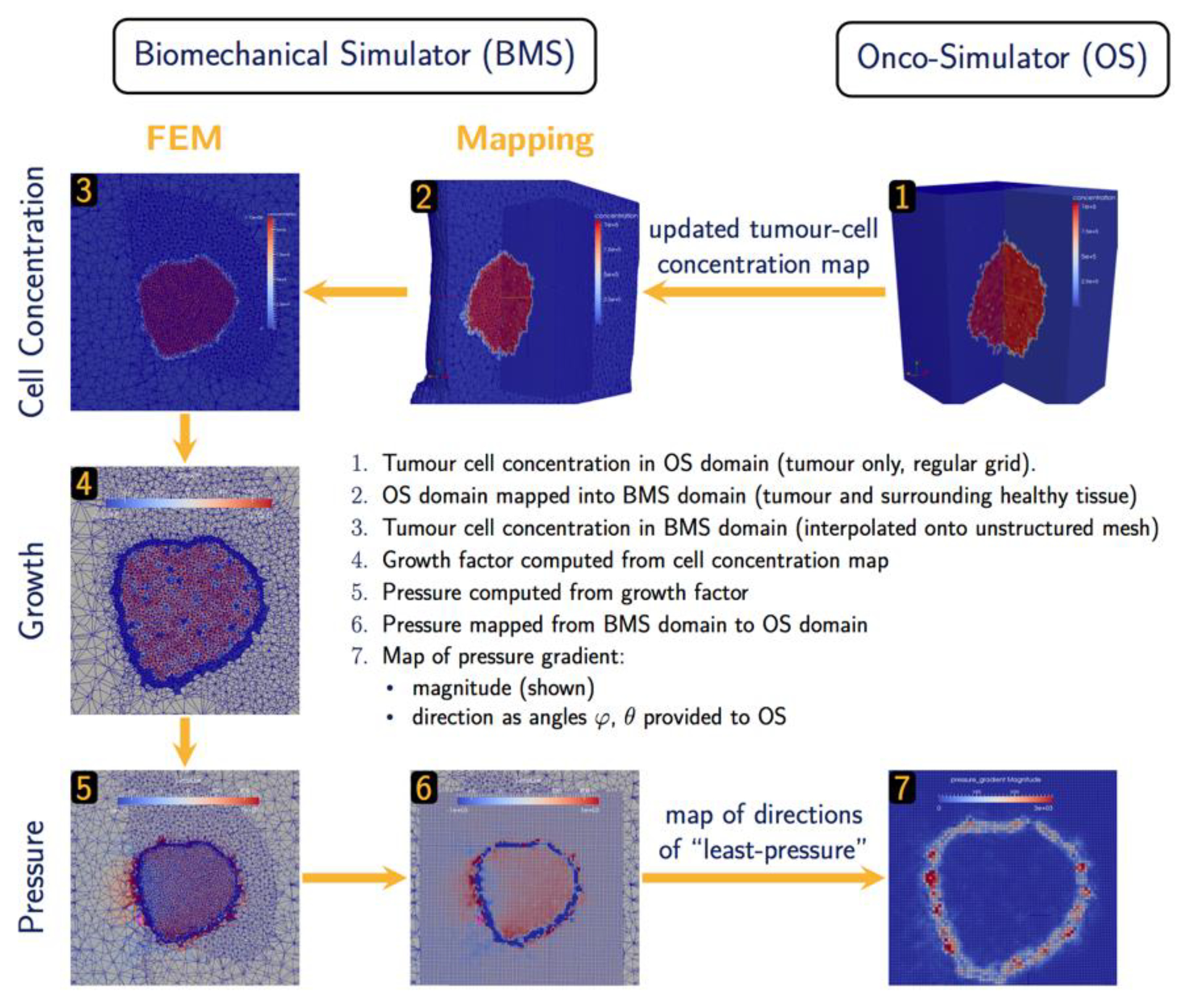
The hyper-modelling scenario dictates an iterative tightly-coupled communication scheme between the Oncosimulator (OS) and the Biomechanics simulator (BMS) (Figure 2 and Figure 3). The dynamic coupling is implemented via MUSCLE as previously described. The Oncosimulator computes cell proliferation in the case of free growth or cell loss in the case of treatment. Starting from an initial spatial map of cancer cell concentrations, BMS receives an (updated) tumor cell concentration map from OS in each time step. BMS and OS operate on distinct domains (OS: tumor only; BMS: tumor & healthy tissue) and discretization (OS: regular grid; BMS: unstructured mesh). Therefore, OS cell concentrations are first mapped into the BMS simulation domain before spatial maps of local tumor-induced volumetric growth can be computed. As the predicted mechanical stresses are intended to inform the spatial redistribution of existing tumor cells, we define the “growth” strain relative to a fixed maximum carrying capacity , below (above) which additional tumor cells may still be accepted (will be rejected) in a region of interest:
Tumor-induced strain assumes positive (negative) values when the local tumor cell concentration exceeds (is less than) the maximum carrying capacity. From this strain map, tumor-induced mechanical stresses (x) are computed using a linear-elastic material model with tissue-specific mechanical parameters, Young’s modulus and poisson ratio . The resulting pressure field is then mapped back from the unstructured grid of the BMS simulation domain into the regular grid of the OS where the “direction of least-pressure” is computed as the normalized negative pressure gradient:
This information is returned to OS where it informs the movement and redistribution of tumor cells. Both models and their joint application (not as separate components) have been tested successfully for brain tumor simulation [26].
Figure 3.
Data exchange and Computation in BMS-OS coupled execution.
2.3. Tumor- and Patient-Specific Parameterization
The parameterization of component models accounts for the observed interpatient variability for both NSCLC adenocarcinoma and Wilms tumor. By incorporating the molecular information of a patient and by properly adjusting model parameters a wide range of genetic, anatomical, tumor growth and tumor response profiles can be reproduced, as described below per component model.
2.3.1. Molecular Hypomodel
Micro-RNAs, short non-coding RNAs that regulate gene expression post-transcriptionally, play critical role in various forms of cancer. Normalized tissue and serum miRNA expression data of a patient are utilized to adjust the initial levels of the nodes of our networks. In particular, we identify the 5-10 miRNA which are overexpressed in particular patient data. Using miRTarBase [33], we are able to obtain the target proteins of these miRNA. The combined molecular model is run with lower levels of activity or concentration for these target proteins, determined based on the expression levels of miRNA with respect to control. For lung cancer, the model additionally, incorporates the sequencing information by considering the mutational status of EGFR, KRAS, BRAF, and AML/ALK. Hence, the final outcomes are tailored to the particular expression profile of the patients to generate clinically useful outcomes.
For WT, nodes are constrained in a similar fashion, based on the drug interactions. In total, we consider doxorubicin, vincristine, and actinomycin. For each type of chemotherapeutic drug there exists literature published cell kill rates which are uniformly applied for all patients. We aim to obtain an adjusted cell kill rate that takes into account patient specific genetic variation. To do this we assume that the effect of drug on cell survival follows a Poisson distribution so that the fraction of cells killed (CKR) is given by where k is a rate constant that is proportional to the cell kill probability. Using subscripts ‘lit’ and ‘adj’ for literature and adjusted cell kill rates we get and . Then the two CKRs are related through the following equation:
The ratio is obtained from simulation for a patient and a control where control indicates no miRNA based initialization of the model. For a combination of drug we assume additivity of rate constants (probabilities) instead of additivities in cell kill rates which is commonly used in literature.
The effect of radiation dosage is implemented through the linear-quadratic model (LQ) [34]. Radiation dosage introduces DNA single and double strand breaks which activates the p53 mediated DNA repair and apoptotic pathways. Due to the discrete nature of our p53 mediate DNA damage model, we are only able to account for the dose independent part (the linear term involving α). Future version will aim to account for the dose dependent part as well which requires a more detailed model which takes into account the various double strand DNA repair mechanisms. In brief, the linear-coefficient is used to constrain the node that regulates the p53 activation in a radiation dose-dependent manner. In particular, we activate the ATM kinase levels according to a probability exp(-α*D). The survival calculated by the model is then modified by the quadratic term involving β. The values of α and β are obtained from the literature.
Finally, the model is run based on the input miRNA and treatment and averages over several tissue conditions such as growth factor levels and receptor expression. An average as well as a distribution of cell growth, cell senescence and cell kill probabilities are obtained for a given patient. The average cell kill probability is translated to cell kill rate (i.e., fraction of cells killed) that is passed on to the multi-modeler framework.
2.3.2. Oncosimulator
The Oncosimulator accounts for the diverse proliferative behavior observed between tumors based on the balance/interplay between active proliferation, reversible dormancy and cell loss due to differentiation, apoptosis or nutrient/oxygen deprivation. However, there is lack of patient-specific data directly linked to the related model parameters. Some experimental data may only suggest plausible value ranges. To overcome this limitation a parametrization methodology has been developed that fits/adapts model predictions to macroscopic clinical proliferation features. We consider that a set of model parameter values constitutes a virtual tumor. The parametrization methodology aims to derive a group of virtual tumors that constitute solutions to the same adaptation problem and efficiently cover the parameter space. These virtual tumors have common a predefined tumor- and patient-specific proliferation profile but, in general, will differ in their treatment response and long-term behavior. The parameter space can be efficiently covered by exploiting computationally low-cost, statistical sampling methods, such as latin hypercube sampling (LHS). If consistent results can be demonstrated for the considered set of virtual tumors (e.g., a clinically significant volume reduction in all cases when applying a specific schedule), this result may be considered robust to the uncertainty in parameter values.
Herein, the proliferation profile of a tumor is described by: a) the doubling time, Td, of tumor volume, b) the growth fraction (GF). To perform personalized predictions, Td can be estimated based on the observed tumor volume increase between two successive imaging examinations, e.g., MRI or CT scans, prior to treatment [S3 in [35]]. GF can be determined by immunohistochemistry for the Ki-67 antibody in biopsies or resected specimens. In the case of non-availability of personalized data, a literature survey can provide biologically reasonable and tumor-specific reference values or value ranges.
Constrains related to other proliferation features of the virtual tumor, i.e., the fraction of stem cells, necrotic and apoptotic cells are also imposed. Value ranges of these critical features informed by clinical studies in literature are utilized.
The parametrization methodology along with the mathematical derivations used to link proliferation features with model parameters are presented in Appendix A. More information can be found in [35,36].
2.3.3. Metabolic Hypomodel
It has been shown that aerobic glycolysis in NSCLC is promoted through oncogenic mutations in two critical proteins, K-RAS and EGFR [37,38]. Ras-driven cancer cells display increased glucose uptake and aerobic glycolysis that support both nucleotide biosynthesis and protein glycosylation for growth signaling. However, it should be noted that high heterogeneity in metabolism proteome has been observed i) compared to normal lung tissue, ii) between lung subtypes and iii) between primary and metastatic lung cancer.
In order to construct a tumor-specific metabolic model in a simplified manner, we included constraints in the metabolic reactions of the model, which are associated with bibliographically reported differentially expressed metabolic genes/proteins in these tumors. mRNA levels cannot accurately determine enzyme concentrations as inaccuracies in experiments, post-translational modifications and other effects might occur. However, they can determine an upper bound on the amount of available enzyme concentrations. In particular, enzyme levels, Ei, bound the fluxes of the corresponding metabolic reactions vi through vi =Kcati Ei, where Kcati corresponds to the enzyme’s turnover number. However, in the absence of quantitative information, metabolic reactions catalyzed by up-regulated metabolic proteins/enzymes, are constrained to carry non-zero fluxes via a lower bound, which is set equal to 0.1umol/mgDW/h unless stated otherwise, for all the involved reactions. Different bounds have also been tested. It is important to mention that the level of flux bound substantially alters the metabolic capabilities of the cells. Downregulated genes constrain the corresponding reactions via an upper bound, which is usually set equal to zero unless stated otherwise.
An extensive omics analysis [37] integrating DNA, RNA and proteomics data from normal lung, patient primary tumors and primary tumor-derived xenograft tumors revealed sets of proteins that are consistently up- or downregulated across tumors, recapitulated in xenograft tumors and their associated genes map into regions of focal amplification or deletion respectively. This DNA->RNA->protein association indicates a response to selective pressure driving cancer phenotype. From the reported metabolism proteome clusters in [37], we used specific clusters of proteins (Table 2) consistently upregulated in LADC (cluster index: C15) and LSCC (cluster index: C10) to constrain the corresponding metabolic fluxes of the genome-scale metabolic network. It is also important to mention that individual proteome clusters have been correlated with overall survival in cancers other than NSCLC.
WT is believed to arise from the malignant transformation of renal stem cells that abnormally persist after embryogenesis and maintain embryonic differentiation capacity. Although there are a few studies that have shown metabolic alteration related to glycolytic phenotype in WT, unfortunately, there are no thorough studies currently available, which have investigated the metabolism of WT in detail. There is only indirect evidence from the genes altered in WT that there are alterations of cell metabolism. Thus, in the absence of bibliographic or other data, we use the generic cancer metabolic model to describe WT metabolism, which can be supported by the fact that Wilms’ tumor cells are believed to derive from pluripotent embryonic renal precursor cells.
Figure 4 summarizes the output variables for different glucose concentrations and different phenotypes. Although the glucose uptake rates (Figure 4c) are very similar among the different phenotypes, their proliferation time (Figure 4a) as well as the lactate production (Figure 4b) are substantially different for the different concentrations of glucose.
2.3.4. Vasculature Hypomodel
Although the model has a physical basis, determination and physical interpretation of parameter values (, , , , ) is challenging. In practice, these parameters should be treated in a phenomenological manner and used in fitting model predictions to observed clinical tumor growth (or shrinkage) rates. Discrimination of the relative influence of delivery by the vasculature and consumption by cells may be aided by additional observations of tumor micro-vessel density, vascular function through functional imaging or cell numbers by functional imaging. However, this has not been performed to date.
In order to obtain reasonable estimates for these parameters for model evaluation, literature values based on observations in tumor spheroids are adopted [39]. Within the hypermodelling framework dependent components use glucose concentrations to predict cell proliferation rates in the tumor. Although the mechanism of glucose consumption by cells also depends on oxygen availability [39], to preserve the simplicity of the model it is assumed that the diffusing nutrient is glucose and glucose consumption is independent of oxygen concentration. Parameter values are shown in Table 3.
2.3.5. Biomechanics Simulator
The mechanical response evoked by a growing tumor depends on its mechanical growth environment which is defined by the surrounding healthy tissues, the tumor’s shape and location, as well as mechanical constraints. The BMS simulator component supports two levels of parameterization to represent (1) different simulation scenarios, such as tumors growing at different body sites, and (2) the patient-specific geometry in any of these scenarios.
In each tumor growth scenario, we identify those tissues that are expected to make a distinct contribution to the tumor’s mechanical landscape, either because of their immediate vicinity to the developing tumor or because of their distinctly different mechanical properties. Average bulk values are assumed for other tissues. As mechanical boundary conditions, we assume the movement of nodes on the outer surface of the BMS simulation domain to be fully constraint. In both hyper modelling scenarios, the BMS simulation domains are chosen to be significantly larger than the actual tumor growth domain (provided by OS). Scenario-specific tissue types and mechanical properties are listed in Table 4 for the WT and the NSCLC scenarios.
While material parameters and boundary conditions are assumed identical across patients within a simulation scenario, differences in patient anatomy are accounted for by solving the equations of continuum elasticity on a patient-specific domain. These personalized computational models are created by first segmenting the region and tissues of from clinical imaging of each patient. From the segmentations of each patient’s anatomy, tetrahedral meshes are generated using an in-house C++ tool based on open-source libraries. Figure 5 and Figure 6 illustrate patient-specific BMS simulation domains for one exemplary patient of the WT and NSCLC scenario, respectively.
3. Results
3.1. Assessing Personalized Predictions for NSCLC Adenocarcinoma: A Proof of Concept Study
A 63-year-old female patient with a past history of lung cancer is considered in the present study. The patient was followed-up and treated at the Institute of Pathology of the University Hospital of Saarland. The study involves the progression and response to radiation treatment of a cancer recurrence that the patient developed.
Treatment schedule considered: The patient received external radiation of the right upper lobe. Four fractions of 15 Gy were given, once a day, three days/week. The radiation schedule considered is detailed in Appendix C.
Patient-specific data: Histological examination of the resected primary section revealed NSCLC adenocarcinoma of stage IB disease (pT2aN0M0) (TNM Classification of Malignant Tumors, 7th ed.) with acinar growth patterns (grade II). Proliferative index determined by Ki-67 labelling was 23%. Mutation analysis revealed the presence of the KRAS mutation Gly12Cys, but no EGFR, BRAF, ALK or ROS-1 alterations. Furthermore, tumor and normal lung tissue samples were analysed for the expression levels of 2549 miRNAs. Values are considered in the present study using quantile normalization [40].
Approximately three years after surgery, successive CT scans show the appearance and progression of a recurrence. Two CT imaging sets of the recurrent cancer acquired three months and one week before the onset of radiotherapy are available for study purposes. A follow-up with CT scan one year after irradiation revealed no tumor presence in the treated area.
Due to the non-availability of biopsy-related data, as a first approximation, the mutation data, miRNA expression values and the Ki-67 proliferation index of the recurrent cancer are considered the same as the ones of the primary tumor (time point T0). The Hypermodel also considers the applied radiotherapeutic scheme (dose, radiation instants) and the 3D image of the tumor as reconstructed from the segmented CT imaging data. In the absence of volumetric data that allow the delineation of any tumor metabolic subregions, segmentation has been restricted to the boundary of the tumor. Hence, the virtual tumor is assumed homogeneous with a shape compliant to the reconstructed tumor image.
Predicted cell kill rate: The predicted cell kill rate from the molecular model was compared with that obtained from the empirical LQ model (Table 5). We observe that the predicted cell kill rates converge at higher radiation dosages but molecular model predictions are lower compared to the LQ model at lower dosage fractions. The results obtained from the molecular model are averages over various growth factor and time scale considerations taking into consideration the molecular profile of the patient.
Predicted treatment outcome: The clinical questions addressed by the hypermodel concerns the prediction of tumor recurrence and in the case of recurrence, to predict the volume of the tumor one year following the completion of tumor irradiation. The progression ‘phase’ of the recurrent tumor before irradiation is used to adapt the Lung Oncosimulator. More specifically, a group of virtual tumors that constitute solutions to the same adaptation problem and efficiently cover the parameter space are derived. The following proliferation constrains/assumptions have been exploited: a) the virtual tumor implementations must have a growth fraction (GF) equal to the proliferation index (Ki67) of the patient (=0.23), b) the volume doubling time must be around 370 days and c) the population composition should be within the value ranges reported in Table 6. Furthermore, the ranges of the model parameters considered are given in Table 6. The doubling time has been estimated based on the observed volume increase between the two available volumetric data before the radiation therapy. At a second step the Oncosimulator is run to simulate tumor progression and treatment response and predict recurrence and tumor volume after irradiation.
LHS has been run to generate 200 combinations of parameter values that fulfill the above requirements, following the methodology described in section 2.3.2. Combinations that result in biologically non-relevant tumors e.g., negative cell class transition rates Psleep and RNDiff, or in tumors with non-relevant proliferation dynamics e.g., stem cell fractions out of range, are excluded.
The first clinical question is addressed by computing the tumor cure probability (TCP), which is the probability that no clonogens survive after treatment [50]. We have adopted the Poisson model of TCP, which is considered a good approximation when the surviving fraction is << 1 [61], as in our clinical case: TCP=exp(-N), where N is the average number of surviving clonogens or cancer stem cells (CSCs) at the end of treatment. In our case, N is derived based on the execution of the hypermodel. In particular, because the Oncosimulator explicitly models the proliferation and treatment-induced death of CSCs, the number of CSCs that remains at the end of the radiation treatment can be computed for each virtual tumor. The number of remaining CSCs depends on their initial number. The latter is determined based on initial tumor volume, assumed tumor cell density (106/mm3) and the value of OS input parameters related to the kinetics of CSCs. Proper adjustment of the consider value ranges ensures that the fraction of CSCs is within the range of TIC (tumor initiating cells) frequency reported in literature (Table 6) for the majority of the virtual tumors returned by the LHS. Virtual tumors having an initial frequency of cancer stem cells beyond this range are excluded from the analysis.
Three scenarios are demonstrated here. In all scenarios the cell kill rate of cells in the all phases is considered equal to the estimation of the molecular component for the specific patient and radiation dose considered. Moreover, the withdrawal of cells in a quiescent phase, as a means to adapt to the local nutrient (glucose) conditions, is regulated by the vasculature and metabolic components. A sufficient average vessel density and glucose consumption rate is considered because the presence or extent of necrosis, which is associated with the local disappearance of blood vessels, is usually low in this histological type [58,59]. The first scenario considers the dose that was actually administered (15 Gy), while the second scenario corresponds to a lower radiation dose (10 Gy). In the third scenario, radiation therapy is given one month earlier.
Figure 8 display the box and whisker plots of the estimated TCP and the predicted tumor volume one year following radiotherapy for the three clinical scenarios. In the first scenario that exploits all available imaging, treatment and molecular data, a TCP close eto zero is estimated (median TCP: 4*10-12, IQR: 2*10-22 – 7*10-5), suggesting that the tumor will recur. The volume of the predicted lesion is approximately 0.91 mm3 (median: 0.908, IQR: 0.909-0.912) at the time point of the final CT acquisition. The predicted volume size is below the detection limit [62] for all virtual tumors implemented. Administration of a lower dose per radiotherapy session (scenario 2) would result again in no local control (TCP: 0), while the predicted tumor size is much larger (median: 78 mm3, IQR:77-79 mm3). If radiotherapy would be given one month earlier (scenario 3), TCP wouldn’t improve (median: 7*10-12, IQR: 7*10-20 – 9*10-6).
Summarizing, the hypermodel predicts (scenario 1) a tumor of an equivalent diameter approximately 0,97 mm i.e., a tumor not easily detected. Based on patient data no visible tumor exists one year after irradiation. Even-though hypermodel predictions seem consistent with reality, follow-up data beyond this period would be needed to properly validate the hypermodel, for the specific clinical case.
3.2. Clinical Adaptation and Partial Validation of the Hypermodel: A Proof of Principle Study for Wilms Tumor
Two clinical cases of Wilms tumor have been selected for the present study. The patients were diagnosed and treated at the Department of Pediatric Oncology and Hematology of the University Hospital of Saarland. The study involved the response to combination chemotherapy.
Treatment schedules considered: Both patients received preoperative chemotherapy with a 4-week regimen of vincristine (1.5 mg/m2, maximum 2 mg) and actinomycin D (45 mg/kg IV, maximum 2 mg) according to the SIOP 2001/GPOH clinical trial for unilateral stage I-III nephroblastoma tumors. (Appendix C). For Case 1 only schedule was available. Dosage was assumed based on other patients.
Patient-specific data: Because of the fragile nature of Wilms tumor, no biopsy is performed in clinical practice and the diagnosis is always made after the surgery. For the cases considered, the histological reports of the resected tumors were not available.
The hypermodel considers the normalized serum miRNA data, the applied chemotherapeutic scheme (dose, administration times) and the 3D image of the tumor as reconstructed from the segmented MRI imaging data. Two MRI imaging sets of the tumor acquired before and after chemotherapy are available for the study purposes. Because of lack of macroscopically distinct tumor subregions, the virtual tumor is assumed homogeneous with a shape compliant to the reconstructed tumor image.
Predicted cell kill rate: The cell kill rates predicted by the molecular model based on the normalized miRNA data are depicted in Table 7. Molecular data model a moderate response to combined chemotherapy for cases 2, while a high CKR is computed for case 1.
Assessment of proliferation profile: The hypermodel is applied to estimate the proliferation profile of the examined clinical cases. The following tumor proliferation features have been considered based on literature: a. volume doubling time: Td=11 days, 25 days, 40 days, b. growth fraction: GF = 10%, 25%, 50% and c. cell proliferation times = 13.1h, 20h, 50h corresponding to high, moderate and very low glucose concentration (Figure 4a), leading to 27 proliferation profiles i.e., pairs of (Td, GF, cell proliferation time). The value range of the input parameters are reported in Table 8. Only parameters related to free growth are varied. Cell kill rates are fixed to the patient-specific estimates from the molecular model (Table 7). LHS has been run to generate 60 virtual tumors (combinations of parameter values) for each pair of (Td, GF, cell proliferation time). Combinations that result in negative cell class transition rates, namely negative Psleep and RADiff, are excluded. For each virtual tumor, the Oncosimulator simulates the therapeutic plan of each clinical case (Appendix C) and the treatment induced volume reduction is predicted. The real chemotherapy-induced shrinkage of tumor volume is compared against the predicted volume reduction to determine the proliferation profiles that are compatible with each clinical case.
The boxplot of the predicted volume reductions for each combination of Td, GF and cell proliferation time is depicted in Figure 9. The tumor volume doubling times cover the entire value range reported in literature. The growth fractions chosen approximately correspond to median values for different histological types of WT [67,68]. The results clearly demonstrate the potential of the integrative hypermodel to predict tumor shrinkage following proper adaptation. In both cases, there are proliferation profiles that are consistent with the observed tumor behavior. For case 1 most virtual tumors suggest a high tumor shrinkage. In case 2 proliferation profiles not consistent with the observed behavior are evident. It is noted that for the specific predictions the only personalized data utilized that could affect the predicted outcome were the serum miRNA expression data. They were used by the molecular model to assess chemosensitivity. The rest of the hypomodels utilized cancer-specific knowledge. The results demonstrate that the increased chemosensitivity of case 1 was successfully captured. Studies of this type can be used to link proliferation activity with response taking into consideration the sensitivity profile of the patient to therapy.
3.3. Assessing Evolution of Tumor Shape and Position
Available clinical medical images at two time points (t1, t2) were registered using a rigid registration procedure in order to establish a common spatial reference frame, facilitating comparison and analysis. Then, the position of the center-of-mass (COM) was computed for both images at the initial time point(t1), the second time point (t2) and at the various simulation timesteps ts,i between t1 and t2. The spatial agreement between the simulation and reality is assessed by measuring the distance between the tumor centre-of-mass positions of the simulated tumor at each simulation time steps ts,i and the center of mass at the final imaging time point (t2). This distance metric serves as a measure of how well the simulation aligns with the actual imaging data.
This assessment strategy was applied to results of the fully integrated WT and NSCLC hypermodels. Figure 7 illustrates 3D shape and position of the simulated tumor in comparison to the actually observed tumor. For the lung scenario medical clinical images at time of diagnosis (t1) and after three months of free growth (t2) were acquired. For the Wilms tumors scenarios, medical imaging was acquired at time of diagnosis (t1) and after the completion of administered chemotherapy scheme (t2). During the simulation period, tumor volume increases in the Lung scenario and decreases in the WT scenario. The simulated free growing tumor in the lung scenario maintains a compact shape, in agreement with observation. Its simulated and observed position at the second imaging time point are approximately 2 cm apart. Likewise, the COM distance remains in the range of about 2 cm for the two selected WT cases. Visual comparison of tumor shape shows that the simulated tumor does not shrink isotropically to a compact bulk tumor with smaller radius as expected from the segmentations of the second imaging time points. Instead, the tumors appear to dissolve from one side, forming a porous and partially disconnected structure.
4. Discussion
The presented multi-scale hyper modeling framework combines subcellular processes related to cell proliferation and cellular response to therapeutic agents, as well as macroscopic processes such as biomechanical interaction between healthy tissue and tumor. Two prevalent cancer types, Wilms tumor and non-small cell lung cancer, were addressed, considering chemotherapy and radiation therapy as treatment modalities. The application of this framework aimed to address different clinical questions related to tumor shrinkage after neoadjuvant therapy and tumor recurrence.
In clinical practice, the detection limits of imaging modalities, underscores the importance of combining heterogeneous data for accurate lesion characterization. In lung, radiological assessments alone may not suffice in discerning small lesions e.g., up to 3mm. Integrated analyses are necessary for a timely distinction between tumors from other condition such as infections or scars. Moreover, accurate tumor localization is relevant for surgical planning, particularly in procedures like nephron-sparing surgery. Knowledge of vascular pathways and potential adherence to other organs like liver, spleen, pancreas and colon is vital for optimizing patient outcomes and minimizing risks. Finally, traditional therapeutic advancements in clinical settings predominantly rely on randomized clinical trials, which aim to identify favorable treatment outcomes on average. However, patient responses to therapies often vary significantly from this averaged behavior. Integrated approaches like the ones presented here can be of great clinical value in determining drug effectiveness, dosage and duration as well as investigating development of resistance to drugs and effect of intra and inter-tumoral heterogeneity. Multiscale cancer modeling holds promise in elucidating why certain treatments fail while others effectively control tumor progression, as well as why a specific therapy is effective only in a subset of patients. Eventually, by training the model using individual patient data, a more precise depiction of disease progression kinetics can be attained.
At molecular level, the p53 mediated signaling pathways are particularly important in determining tumor cell response to DNA damage chemotherapeutic drugs like doxorubicin and vincristine as well as radiation therapy [71]. In the present work, we presented an integrated molecular model to model key cell signaling pathways operating at different time scales – a well-recognized challenge in the field. We model the p53 mediated DNA damage response pathway and we refine its predictions by running a model of the ErbB receptor mediated Ras-MAPK and PI3K/AKT pathways. Information is passed across the identified interfaces in both directions. In order to consider the effect of patient-specific molecular profiling, we have also incorporated the miRNA expression and various mutation data to re-normalize the initial expression levels of corresponding mRNAs to a given patient. In doing so, however, we have also taken into account the heterogeneity of the microenvironment and have adopted an ensemble of models approach by averaging over multiple conditions of receptor expression, growth factor availability, and nature of the memory coupling signaling and transcriptional modules. The aim is to provide a mechanistic foundation to the more empirical models to obtain patient specific cell kill rates under particular dosage conditions. The future work will be focused on performing a detailed sensitivity analysis to simulate the inherent tumor heterogeneity and also the effect of various mutations and subject the framework to clinical validation.
The obtained cell kill rate was directly incorporated as an input to the Oncosimulator. The Oncosimulator serves as an integrator, effectively bridging scales and facilitating the “exposure” of molecular mechanisms to the scale where the outcome is formulated. The Oncosimulator is build based on cancer stem cell hypothesis and accounts for tumor repopulation during and after treatment assuming different tumor proliferation dynamics and varying degrees of adaptation to nutrient-deprived conditions. As tumor grows well-vascularized regions providing sufficient nutrients to cancer cells can coexist with nutrient-limited regions within the tumor mass. In this work, glucose is assumed to be the only limiting resource, although oxygen can also be incorporated as well as glutamine. The metabolic component models the dependence of glucose uptake on glucose concentration, using Michaelis-Menten kinetics at genome scale. The model encapsulates the metabolic adaptations exhibited by highly proliferating human cancer cells and provides information to the Oncosimulator regarding the cell proliferation rate given the available glucose. The local concentration of glucose is described by the vasculature model.
A simple vasculature model was constructed as the first to be used in the development, verification and validation of the WT and NSCLC multi-modeler hypermodels. More detailed models, as described subsequently, can be readily incorporated in the framework if justified by available clinical data. First of all, several ‘nutrient’ fields can be considered such as oxygen and glutamine. In reality, when used to model glucose transport, oxygen availability should also be accounted for, as per [72]. Another aspect is that the metabolic hypomodel uses an independent model of glucose consumption. In theory, the rate of glucose consumption from the metabolic model could be passed back to the vasculature component and used to update glucose concentrations. Moreover, the vasculature is assumed to be ‘static’ in the current model, in that it does not evolve in time. If justified by available data temporal evolution of the vasculature can be easily included. In addition to the tissue-scale transport model used in the clinical demonstrators, a range of more spatially resolved models of transport in tumor micro-vessels have been developed using Chaste [15]. These models can be used to inform the hypomodel used in the present work.
The hypermodel is found to reproduce realistic tumor shapes in growth scenarios (Lung), whereas shrinkage scenarios (Nephroblastoma (WT)) tend to result in tumor shapes that have a more ‘diffuse’ appearance than those observed. The hypermodel achieved a good prediction of tumor position in the simulated cases. The following limitations may explain the observed discrepancies and could be the subject of future research. A critical issue for Biomechanics Simulator is the uncertainty in mechanical tissue parameters (not patient-specific) and the lack of well-defined boundary conditions for mechanical computations that are particularly difficult to establish for the WT and Lung scenarios. Furthermore, the evaluation relies on image registration techniques to compare simulation results to imaging data at a later time point. This process introduces an uncertainty in the relative positioning of the tumors. To reduce the importance of this uncertainty in future studies, the use of fixed anatomical markers as reference within the respective imaging frame could be investigated. Another limitation is related to the complexity of the coupling between OS and BMS. Mapping of the pressure (direction of least-pressure) field computed by BMS into the discrete model of OS is challenging, as is the update of BMS with OS cell concentration values. Accuracy in both steps is affected by interpolation. Mesh creation from image segmentations and mapping of 3D parameters distributions between domains, are a commonly used in Finite Element or Finite Difference based simulations. These ‘convenience functions’ are crucial for functioning simulator components. We believe that each of these functionalities could be well encapsulated in a standalone hypo-model in the future. This would not only greatly facilitate the creation of new personalized FEM models and the parameter exchange between other component simulators; it would also ensure consistent handling of these critical simulation and communication aspects across the platform. Finally, morphological changes in the healthy tissue also influence tumor evolution. This aspect is not taken into account by the present hypermodels.
5. Conclusions
Based on the partial validation results and analyses that have been reported in this document, the highly innovative CHIC hypermodels and Oncosimulators appear to possess a great potential for serving as clinical decision support systems (CDS) and/or cores of future in silico trial platforms. However, additional retrospective validation work for the developed hypermodels and Oncosimulators is needed in order to more fully substantiate and support their “candidacy” for undergoing validation through prospective clinical trials. This is a necessary step in order to definitely assess both their clinical validity and clinical value. Further retrospective validation work will be carried out by specific former CHIC partners on a bilateral or small partner group basis. Regarding the eventual prospective clinical validation of the hypermodels, certain exploratory steps have already been taken, including focused discussions within the framework of the International Society for Paediatric Oncology (SIOP).
Author Contributions
Hypermodel conceptualization, G.S., P.B., R.R., H.B. and N.G.; lung and Wilms tumor oncosimulator algorithmic development, G.S, E.K and E.G; lung oncosimulator implementation, E.K.; Wilms tumor oncosimulator implementation, E.G. and E.K.; biomechanics hypomodel, D.A. and P.B.; vasculature hypomodel, J.G. and H.B.; metabolic hypomodel, E.T. and V.S.; molecular hypomodel, A.G. and R.R.; design of the overarching topology of the corresponding hypermodels, E.K., J.G., D.A., E.T., V.S., R.R. and G.S.; preparation and provision of clinical data: N.G., R.B. and E.M.,; lung tumor segmentation: K.N.; image processing & visualization, I.K., N.M., D.K. and F.D.; performed analyses, E.K.; writing—original draft preparation, E.K., D.A., A.G., E.T., J.G., E.G. and G.S. ; writing—editing, E.K.; writing—review, E.G., P.B., R.R., H.B., V.S., N.G. and G.S.; CHIC project coordination, G.S. All authors have read and agreed to the published version of the manuscript.
Funding
The research leading to these results has received funding from the European Union’s Seventh Framework Programme (FP7/2007-2013) under grant agreement n° 600841- “CHIC” [73].
Institutional Review Board Statement
Ethical approval was given by the “Ärztekammer des Saarlandes for retrospective data use of WT and NSCLC patients under 104/10 of 19th August 2013
Informed Consent Statement
Informed consent was given by the parents of children with WT for the retrospective usage of data for research. For the NSCLC all patients of the university hospital were informed and agreed to the surgical procedures and to the histopathological and molecular pathology investigations according to the national lung cancer treatment guideline (“AMWF S3 Leitlinie Lungenkrebs”). A separate “informed consent” document for pathologists was not required by the review board.
Data Availability Statement
The core work of the manuscript was done during the implementation of the European Commission funded project CHIC (Computational Horizons In Cancer (CHIC): Developing Meta- and Hyper-Multiscale Models and Repositories for In Silico Oncology) that took place between 2013 and 2017 (https://cordis.europa.eu/project/id/600841). Since then, significant conceptual processing has taken place, especially in view of the current prioritization of the development and the clinical translation of digital twins, such as the CHIC oncosimulators and hypermodels. In this context, the multiscale clinical data used for the needs of the work reported ceased to be accessible one year after the completion of the CHIC project, in accordance with the consortium agreement and in line with the then applicable ethical and legal provisions, including GDPR. Meta-data are included in Appendix C. Regarding the computer codes, these have been developed and built in house by the modelling partners of the CHIC consortium and are not “open access”, with the exception of the vasculature hypomodel. It is worth mentioning, however, that the CHIC project outcomes were thoroughly reviewed and evaluated by external independent reviewers appointed by the European Commission. The CHIC project was evaluated by the independent reviewers as “excellent”, whereas its outcomes were designated as “great achievements” (https://digital-strategy.ec.europa.eu/en/news/great-achievements-eu-funded-chic-project)
Conflicts of Interest
The authors declare no conflicts of interest.
Appendix A
Parametrization Methodology of the Oncosimulator
The Latin Hypercube Sampling method is used to generate a plausible collection of model parameter values that corresponds to virtual tumors having a common proliferation pattern in terms of volume doubling time, Td, growth fraction (GF). We consider the fraction of newborn cells that enter the G0 phase, Psleep, and the necrosis rate of differentiated cells, RNDiff, as the dependent parameters of this multi-constrained problem. The independent variables comprise the rest of the model parameters that regulate tumor proliferation pattern, i.e., cell cycle time, TC, the duration of G0 phase, TG0, the duration of apoptosis, TA, and the duration of necrosis, TN, the apoptosis rate of stem and LIMP cells, RA, the apoptosis rate of differentiated cells, RADiff, the symmetric division fraction, Psym, the fraction of stem cells that re-enter cell cycle from a quiescent state, PG0toG1, the number of mitoses performed by LIMP cells before becoming terminally differentiated NLIMP, and resistance of stem cells to chemotherapy, CKF, and the above mentioned tumor proliferation features: GF and Td.
The analysis has been performed using the Matlab toolbox. The built-in function ‘lhsdesign’ is run to produce N combinations of the independent model parameters: TC, TG0, TN, TA, RA, RADiff, PG0toG1, NLIMP, α/β. LHS output is modified in the case of parameters with value range other than [0, 1] and parameters of integer type. For input parameters bounded in any range [ap, bp] other than [0, 1], the ‘lhsdesign’ output has been rescaled by applying the formula:
where xp the vector of the N returned values for parameter p. For integer input parameters the rescaled values are rounded to the nearest integer.
For each set of the independent parameter values, parameter Psleep is computed based on the cell proliferation time returned by the metabolic hypomodel as described in section 2.2.2.
Then, Psym and RNDiff, are derived from the following formulas, so as to achieve the given Td and GF.
Initially, the Psym value is computed so as to achieve the given Td:
where α=ln(2)/ Td
RNDiff, is calculated in order to achieve the given GF:
where
Appendix B
Validity Checks of Vasculature Component
An advantage of the simple nature of the adopted hypomodel is that it allows for testing and a clear path for model comparison with clinical datasets. This section overviews verification and testing of the final hypomodel implementation.
For testing it is useful to assume a spherical tumor of radius . Non-dimensionalising Equation (4) with spatial coordinate and concentration gives:
where is a Thiele modulus related to vessel delivery efficiency and is a Thiele modulus related to tumor consumption efficiency. Assuming a 100.0 mm radius tumor, the parameter values in Table 3, a typical cell number of 1.e9 in a region of interest and a vessel volume fraction of 1.0 gives = 160 and = 80, suggesting a reasonably high rate of glucose consumption versus delivery and very high reaction versus diffusion timescales. Converting Equation (B1) to spherical coordinates and dropping accents gives:
with at and at . This can be solved explicitly, giving
Solution values for a range of values of and are shown in Figure A1, along with hypomodel predictions. This serves as both hypomodel verification and a means for identifying suitable parameter values when attempting to describe clinical observations.
Figure A1.
(a) The test geometry for the hypomodel, a 100 mm radius spherical tumor. (b) The predicted dimensionless nutrient field for and . (c) A comparison of the hypomodel predictions versus Equation (B3). There is good agreement, within deviations at due to the use of a regular grid to discretize the spherical tumor.
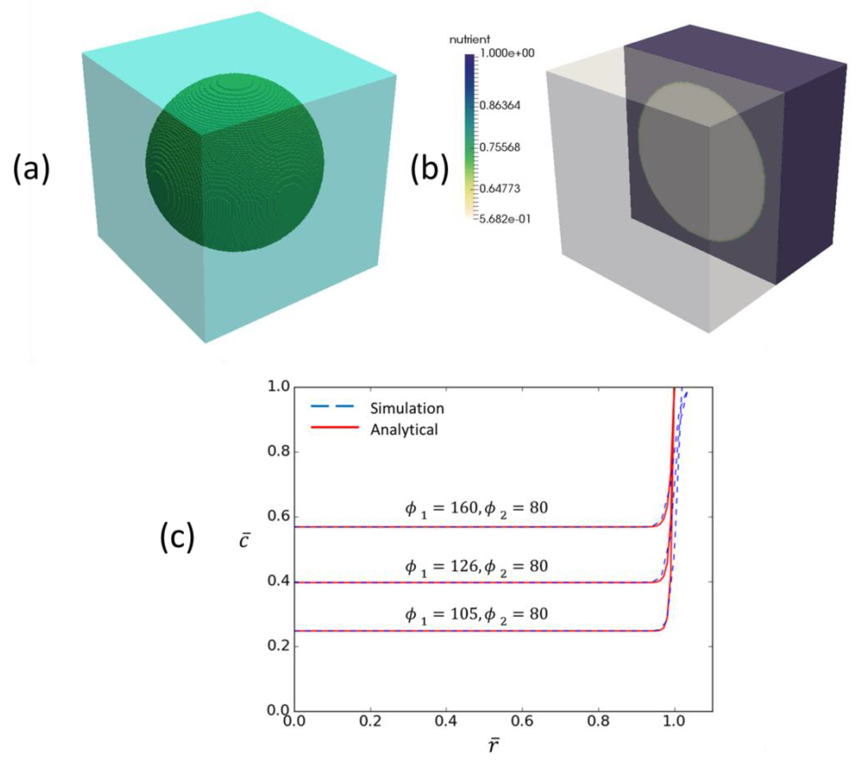
The following model serves as a simple method for relating the hypomodel inputs to tumor growth rate predictions using the dimensional form of Equation (B3), based on a more detailed treatment in [39]:
where s is the tumor cell proliferation rate per unit nutrient concentration. Solution of Equation (B4) following the steps in [39] allows for the estimation of hypomodel parameter values from clinical data by fitting of clinically observed tumor growth rates. In the case of the demonstrator hypermodels and CHIC clinical data, more detailed, integrated, fitting is required.
Appendix C
Clinical Data of the Lung Case Studies Detailed in Section 3
For the Lung cancer case studies detailed in Section 3, three sets of MRI imaging data have been available, two at a time instant prior to chemotherapy and one approximately one year after the completion of radiootherapy. The clinical tumor volumes, as calculated based on the segmentation of the tumors on these imaging sets, are depicted in Figure A2 and Table A2.
The simulation duration and the exact treatment scheme administered for each, as derived from the available clinical data of the patients, are illustrated in Figure A2.
Figure A2.
The simulation durations and chemotherapy protocols for the lung cancer case, presented in the paper (Section 3).
Figure A2.
The simulation durations and chemotherapy protocols for the lung cancer case, presented in the paper (Section 3).
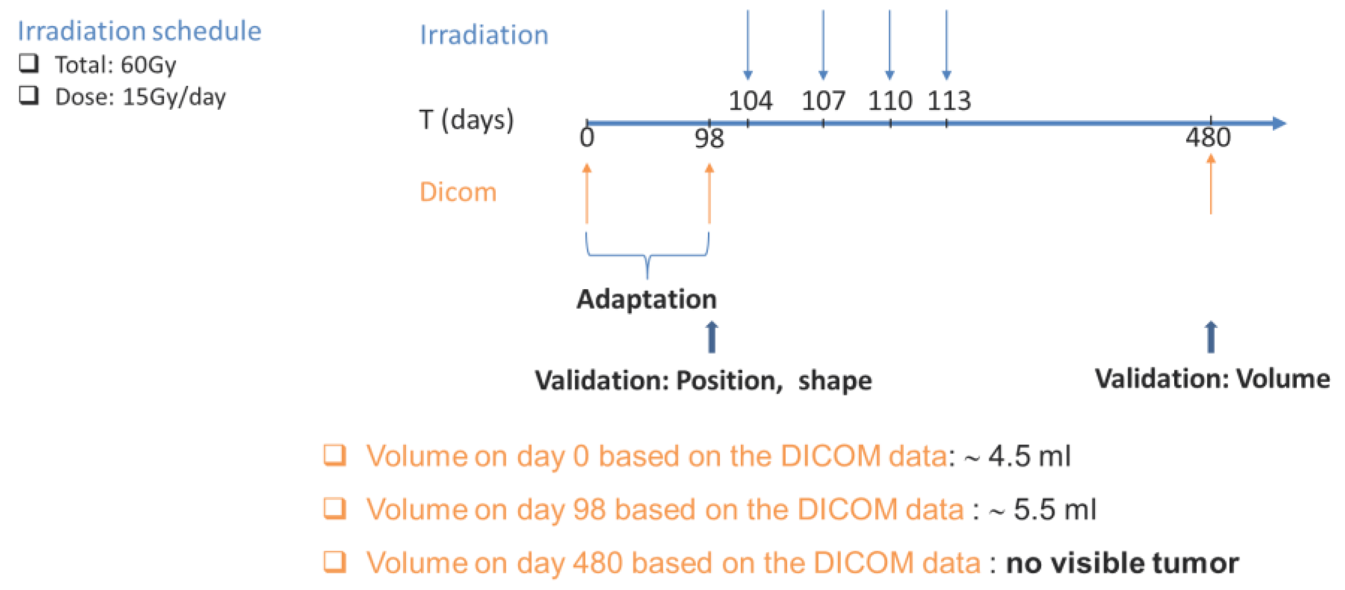
Table A1.
Imaging data information of the lung cancer patients simulated and presented in Section 3.
Table A1.
Imaging data information of the lung cancer patients simulated and presented in Section 3.
| Imaging | VCT (cc) | DVCT (%) | |
|---|---|---|---|
| Case 1 | PRE 1st | 4.5 | 22.22 |
| PRE 2nd | 5.5 |
Clinical Data of the Wilms Case Studies Detailed in Section 3
For the Wilms case studies detailed in Section 3, two sets of MRI imaging data have been available, one at a time instant prior to chemotherapy (t1) and one after the completion of chemotherapy and before surgery (t2). The clinical tumor volumes, as calculated based on the segmentation of the tumors on these imaging sets, are depicted in Table A2.
The simulation duration and the exact treatment scheme administered for each, as derived from the available clinical data of the patients, are illustrated in Figure A3.
Figure A3.
The simulation durations and chemotherapy protocols for Wilms cases, presented in the paper (Section 3).
Figure A3.
The simulation durations and chemotherapy protocols for Wilms cases, presented in the paper (Section 3).
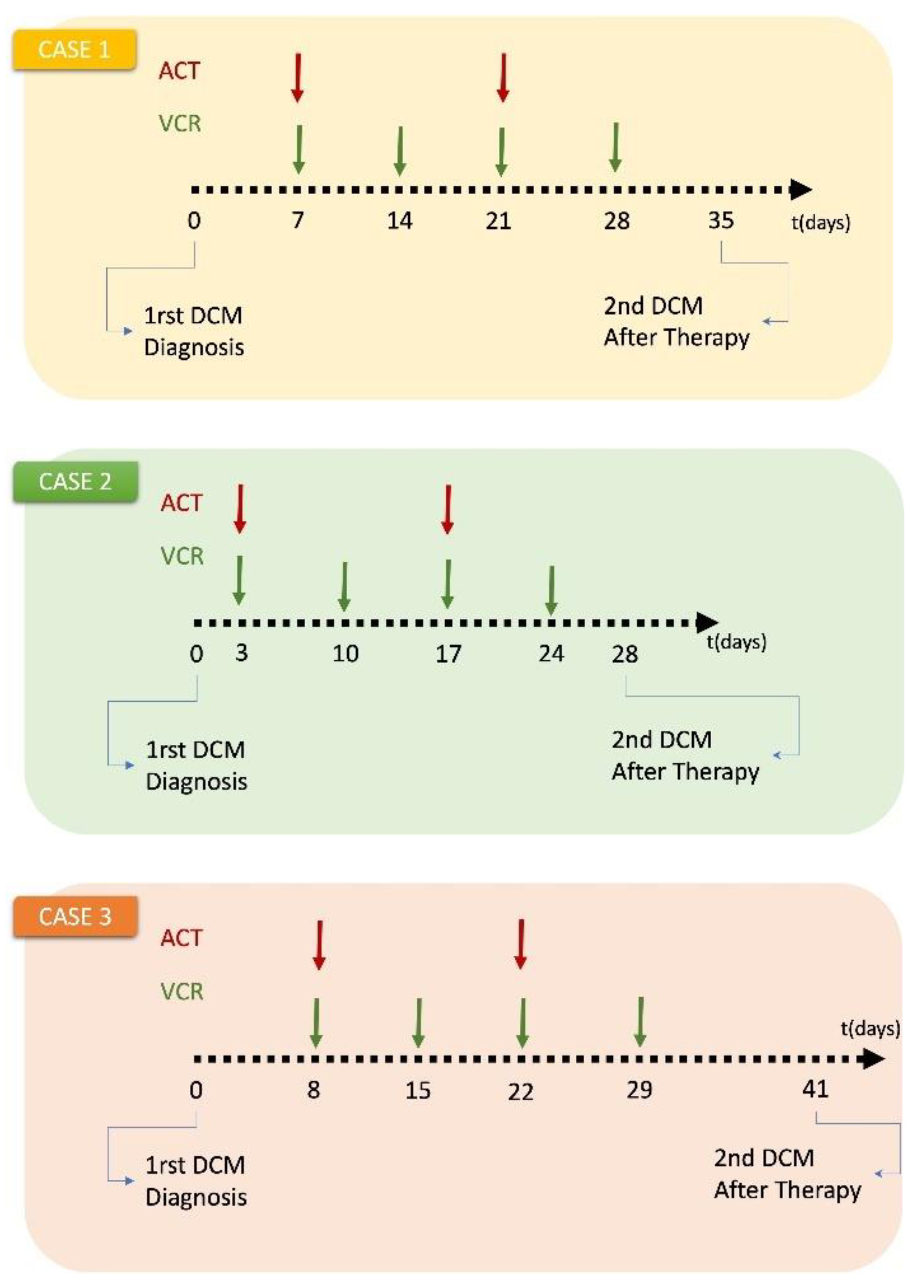
Table A2.
Imaging data information of the nephroblastoma patients simulated and presented in Section 3.
Table A2.
Imaging data information of the nephroblastoma patients simulated and presented in Section 3.
| Imaging | VCT (cc) | DVCT (%) | |
|---|---|---|---|
| Case 1 | PRE | 78.54 | 90.68 |
| POST | 7.32 | ||
| Case 2 | PRE | 109 | 52.29 |
| POST | 52 | ||
| Case 3 | PRE | 754.75 | 80.43 |
| POST | 147.68 |
References
- Goh WWB, Wong L. The Birth of Bio-data Science: Trends, Expectations, and Applications. Genomics, Proteomics & Bioinformatics. 2020;18(1):5-15. [CrossRef]
- Anaya-Isaza A, Mera-Jiménez L, Zequera-Diaz M. An overview of deep learning in medical imaging. Informatics in Medicine Unlocked. 2021;26:100723. [CrossRef]
- Stamatakos GS, Kolokotroni EA, Dionysiou DD, Georgiadi ECh, Desmedt C. An advanced discrete state–discrete event multiscale simulation model of the response of a solid tumor to chemotherapy: Mimicking a clinical study. Journal of Theoretical Biology. 2010;266(1):124-139. [CrossRef]
- Shlomi T, Benyamini T, Gottlieb E, Sharan R, Ruppin E. Genome-scale metabolic modeling elucidates the role of proliferative adaptation in causing the Warburg effect. PLoS Comput Biol. 2011;7(3):e1002018. [CrossRef]
- Borgdorff J, Bona-Casas C, Mamonski M, et al. A Distributed Multiscale Computation of a Tightly Coupled Model Using the Multiscale Modeling Language. Procedia Computer Science. 2012;9:596-605. [CrossRef]
- Viceconti M, Bnà S, Tartarini D, et al. VPH-HF: A software framework for the execution of complex subject-specific physiology modelling workflows. Journal of Computational Science. 2018;25:101-114. [CrossRef]
- http://www.chic-vph.eu.
- Stamatakos GS, Georgiadi EC, Graf N, Kolokotroni EA, Dionysiou DD. Exploiting Clinical Trial Data Drastically Narrows the Window of Possible Solutions to the Problem of Clinical Adaptation of a Multiscale Cancer Model. Zhang L, ed. PLoS ONE. 2011;6(3):e17594. [CrossRef]
- Dionysiou DD, Stamatakos GS, Uzunoglu NK, Nikita KS, Marioli A. A four-dimensional simulation model of tumour response to radiotherapy in vivo: parametric validation considering radiosensitivity, genetic profile and fractionation. J Theor Biol. 2004;230(1):1-20. [CrossRef]
- Borgdorff J, Mamonski M, Bosak B, et al. Distributed multiscale computing with MUSCLE 2, the Multiscale Coupling Library and Environment. Journal of Computational Science. 2014;5(5):719-731. [CrossRef]
- Steel GG, ed. Basic Clinical Radiobiology. 3. ed. Arnold; 2002.
- Chen WW, Schoeberl B, Jasper PJ, et al. Input–output behavior of ErbB signaling pathways as revealed by a mass action model trained against dynamic data. Molecular Systems Biology. 2009;5(1):239. [CrossRef]
- Choi M, Shi J, Jung SH, Chen X, Cho KH. Attractor landscape analysis reveals feedback loops in the p53 network that control the cellular response to DNA damage. Sci Signal. 2012;5(251):ra83. [CrossRef]
- Hahnfeldt P, Panigrahy D, Folkman J, Hlatky L. Tumor development under angiogenic signaling: a dynamical theory of tumor growth, treatment response, and postvascular dormancy. Cancer Res. 1999;59(19):4770-4775.
- Mirams GR, Arthurs CJ, Bernabeu MO, et al. Chaste: An Open Source C++ Library for Computational Physiology and Biology. Prlic A, ed. PLoS Comput Biol. 2013;9(3):e1002970. [CrossRef]
- https://github.com/jmsgrogan/Chic.
- Warburg O. On the origin of cancer cells. Science. 1956;123(3191):309-314. [CrossRef]
- Cairns RA, Harris IS, Mak TW. Regulation of cancer cell metabolism. Nat Rev Cancer. 2011;11(2):85-95. [CrossRef]
- Vander Heiden MG, Cantley LC, Thompson CB. Understanding the Warburg Effect: The Metabolic Requirements of Cell Proliferation. Science. 2009;324(5930):1029-1033. [CrossRef]
- Duarte NC, Becker SA, Jamshidi N, et al. Global reconstruction of the human metabolic network based on genomic and bibliomic data. Proc Natl Acad Sci U S A. 2007;104(6):1777-1782. [CrossRef]
- Ibarra RU, Edwards JS, Palsson BO. Escherichia coli K-12 undergoes adaptive evolution to achieve in silico predicted optimal growth. Nature. 2002;420(6912):186-189. [CrossRef]
- Mahadevan R, Schilling CH. The effects of alternate optimal solutions in constraint-based genome-scale metabolic models. Metab Eng. 2003;5(4):264-276. [CrossRef]
- E. Tzamali, V. Sakkalis, and K. Marias, “The effects of near optimal growth solutions in genome-scale humanME cancer metabolic model,” presented at the Bioinformatics & Bioengineering (BIBE), 2012 IEEE 12th International Conference, Larnaca, Cyprus, 2012.
- Jain RK, Martin JD, Stylianopoulos T. The Role of Mechanical Forces in Tumor Growth and Therapy. Annu Rev Biomed Eng. 2014;16(1):321-346. [CrossRef]
- Helmlinger G, Netti PA, Lichtenbeld HC, Melder RJ, Jain RK. Solid stress inhibits the growth of multicellular tumor spheroids. Nat Biotechnol. 1997;15(8):778-783. [CrossRef]
- May CP, Kolokotroni E, Stamatakos GS, Büchler P. Coupling biomechanics to a cellular level model: an approach to patient-specific image driven multi-scale and multi-physics tumor simulation. Prog Biophys Mol Biol. 2011;107(1):193-199. [CrossRef]
- Bauer S, May C, Dionysiou D, Stamatakos G, Buchler P, Reyes M. Multiscale Modeling for Image Analysis of Brain Tumor Studies. IEEE Trans Biomed Eng. 2012;59(1):25-29. [CrossRef]
- Rikhtegar F, Kolokotroni E, Stamatakos G, Buchler P. A model of tumor growth coupling a cellular biomodel with biomechanical simulations. In: Proceedings of the 2014 6th International Advanced Research Workshop on In Silico Oncology and Cancer Investigation - The CHIC Project Workshop (IARWISOCI). IEEE; 2014:1-4. [CrossRef]
- Abler D, Büchler P. Evaluation of a Mechanically Coupled Reaction–Diffusion Model for Macroscopic Brain Tumor Growth. In: Gefen A, Weihs D, eds. Computer Methods in Biomechanics and Biomedical Engineering. Lecture Notes in Bioengineering. Springer International Publishing; 2018:57-64. [CrossRef]
- http://www.taverna.org.uk/.
- Nik Nabil WN, Xi Z, Song Z, et al. Towards a Framework for Better Understanding of Quiescent Cancer Cells. Cells. 2021;10(3):562. [CrossRef]
- Kolokotroni EA, Dionysiou DD, Uzunoglu NK, Stamatakos GS. Studying the growth kinetics of untreated clinical tumors by using an advanced discrete simulation model. Mathematical and Computer Modelling. 2011;54(9-10):1989-2006. [CrossRef]
- Chou CH, Chang NW, Shrestha S, et al. miRTarBase 2016: updates to the experimentally validated miRNA-target interactions database. Nucleic Acids Res. 2016;44(D1):D239-247. [CrossRef]
- Brenner DJ. The linear-quadratic model is an appropriate methodology for determining isoeffective doses at large doses per fraction. Semin Radiat Oncol. 2008;18(4):234-239. [CrossRef]
- Kolokotroni E, Dionysiou D, Veith C, et al. In Silico Oncology: Quantification of the In Vivo Antitumor Efficacy of Cisplatin-Based Doublet Therapy in Non-Small Cell Lung Cancer (NSCLC) through a Multiscale Mechanistic Model. Komarova NL, ed. PLoS Comput Biol. 2016;12(9):e1005093. [CrossRef]
- Kyroudis CA, Dionysiou DD, Kolokotroni EA, Stamatakos GS. Studying the regression profiles of cervical tumours during radiotherapy treatment using a patient-specific multiscale model. Sci Rep. 2019;9(1):1081. [CrossRef]
- Li L, Wei Y, To C, et al. Integrated Omic analysis of lung cancer reveals metabolism proteome signatures with prognostic impact. Nat Commun. 2014;5(1):5469. [CrossRef]
- Davidson SM, Papagiannakopoulos T, Olenchock BA, et al. Environment Impacts the Metabolic Dependencies of Ras-Driven Non-Small Cell Lung Cancer. Cell Metab. 2016;23(3):517-528. [CrossRef]
- Greenspan HP. Models for the Growth of a Solid Tumor by Diffusion. Stud Appl Math. 1972;51(4):317-340. [CrossRef]
- Faraldi M, Gomarasca M, Sansoni V, Perego S, Banfi G, Lombardi G. Normalization strategies differently affect circulating miRNA profile associated with the training status. Sci Rep. 2019;9(1):1584. [CrossRef]
- Jeong J, Oh JH, Sonke JJ, et al. Modeling the Cellular Response of Lung Cancer to Radiation Therapy for a Broad Range of Fractionation Schedules. Clinical Cancer Research. 2017;23(18):5469-5479. [CrossRef]
- Liu C, Tsao MS. Proto-oncogene and growth factor/receptor expression in the establishment of primary human non-small cell lung carcinoma cell lines. Am J Pathol. 1993;142(2):413-423.
- Masuda N, Fukuoka M, Takada M, Kudoh S, Kusunoki Y. Establishment and characterization of 20 human non-small cell lung cancer cell lines in a serum-free defined medium (ACL-4). Chest. 1991;100(2):429-438. [CrossRef]
- Durand RE, Sham E. The lifetime of hypoxic human tumor cells. Int J Radiat Oncol Biol Phys. 1998;42(4):711-715. [CrossRef]
- Ginsberg T. Modellierung und Simulation der Poliferationsregulation und Strahlentherapie normaler und maligner Gewebe. Als Ms. gedr. VDI-Verl; 1996.
- Chvetsov AV, Palta JJ, Nagata Y. Time-dependent cell disintegration kinetics in lung tumors after irradiation. Phys Med Biol. 2008;53(9):2413-2423. [CrossRef]
- Kerr JF, Wyllie AH, Currie AR. Apoptosis: a basic biological phenomenon with wide-ranging implications in tissue kinetics. Br J Cancer. 1972;26(4):239-257. [CrossRef]
- Gavrieli Y, Sherman Y, Ben-Sasson SA. Identification of programmed cell death in situ via specific labeling of nuclear DNA fragmentation. The Journal of cell biology. 1992;119(3):493-501. [CrossRef]
- Bursch W, Paffe S, Putz B, Barthel G, Schulte-Hermann R. Determination of the length of the histological stages of apoptosis in normal liver and in altered hepatic foci of rats. Carcinogenesis. 1990;11(5):847-853. [CrossRef]
- Rawlins EL, Hogan BLM. Epithelial stem cells of the lung: privileged few or opportunities for many? Development. 2006;133(13):2455-2465. [CrossRef]
- Rawlins EL, Hogan BLM. Ciliated epithelial cell lifespan in the mouse trachea and lung. Am J Physiol Lung Cell Mol Physiol. 2008;295(1):L231-234. [CrossRef]
- Lippmann M. Environmental Toxicants: Human Exposures and Their Health Effects. 3rd ed. J. Wiley; 2009.
- Flindt R. Amazing Numbers in Biology. Springer-Verlag; 2006.
- Pine SR, Ryan BM, Varticovski L, Robles AI, Harris CC. Microenvironmental modulation of asymmetric cell division in human lung cancer cells. Proc Natl Acad Sci U S A. 2010;107(5):2195-2200. [CrossRef]
- Morrison BJ, Steel JC, Morris JC. Sphere culture of murine lung cancer cell lines are enriched with cancer initiating cells. PLoS One. 2012;7(11):e49752. [CrossRef]
- Van Leeuwen CM, Oei AL, Crezee J, et al. The alfa and beta of tumours: a review of parameters of the linear-quadratic model, derived from clinical radiotherapy studies. Radiat Oncol. 2018;13(1):96. [CrossRef]
- Ishizawa K, Rasheed ZA, Karisch R, et al. Tumor-Initiating Cells Are Rare in Many Human Tumors. Cell Stem Cell. 2010;7(3):279-282. [CrossRef]
- Törmänen U, Eerola AK, Rainio P, et al. Enhanced apoptosis predicts shortened survival in non-small cell lung carcinoma. Cancer Res. 1995;55(23):5595-5602.
- Moon SW, Kim JJ, Jeong SC, Kim YH, Han JW. Clinical significance of tumor necrosis and viability in non-small cell lung cancer. J Thorac Dis. 2022;14(4):892-904. [CrossRef]
- O’Neill AJ, Staunton MJ, Gaffney EF. Apoptosis occurs independently of bcl-2 and p53 over-expression in non-small cell lung carcinoma. Histopathology. 1996;29(1):45-50. [CrossRef]
- Zaider M, Minerbo GN. Tumour control probability: a formulation applicable to any temporal protocol of dose delivery. Phys Med Biol. 2000;45(2):279-293. [CrossRef]
- Grannis FW. Limitations of molecular testing in combination with computerized tomographic for lung cancer screening. Nat Commun. 2022;13(1):3890. [CrossRef]
- Groninger E, Meeuwsen-de Boar T, Koopmans P, et al. Pharmacokinetics of vincristine monotherapy in childhood acute lymphoblastic leukemia. Pediatr Res. 2002;52(1):113-118. [CrossRef]
- Hill CR, Cole M, Errington J, Malik G, Boddy AV, Veal GJ. Characterisation of the Clinical Pharmacokinetics of Actinomycin D and the Influence of ABCB1 Pharmacogenetic Variation on Actinomycin D Disposition in Children with Cancer. Clin Pharmacokinet. 2014;53(8):741-751. [CrossRef]
- Theerakitthanakul K, Saetang J, Kruatong J, et al. Senescence Process in Primary Wilms’ Tumor Cell Culture Induced by p53 Independent p21 Expression. J Cancer. 2016;7(13):1867-1876. [CrossRef]
- Royer-Pokora B, Busch MA, Tenbusch S, et al. Comprehensive Biology and Genetics Compendium of Wilms Tumor Cell Lines with Different WT1 Mutations. Cancers. 2020;13(1):60. [CrossRef]
- Berrebi D, Leclerc J, Schleiermacher G, et al. High Cyclin E Staining Index in Blastemal, Stromal or Epithelial Cells Is Correlated with Tumor Aggressiveness in Patients with Nephroblastoma. Westermark P, ed. PLoS ONE. 2008;3(5):e2216. [CrossRef]
- Jurić I, Pogorelić Z, Kuzmić-Prusac I, et al. Expression and prognostic value of the Ki-67 in Wilms’ tumor: experience with 48 cases. Pediatr Surg Int. 2010;26(5):487-493. [CrossRef]
- Craft A. Growth rate of Wilms’ tumour. The Lancet. 1999;354(9184):1127. [CrossRef]
- Middleton P, Banieghbal B, Pitcher R, Schubert P. Radiological response and histological findings in nephroblastoma: Is the any correlation? Afr J Paediatr Surg. 2020;17(3):39. [CrossRef]
- Lee CL, Blum JM, Kirsch DG. Role of p53 in regulating tissue response to radiation by mechanisms independent of apoptosis. Transl Cancer Res. 2013;2(5):412-421.
- Roose T, Chapman SJ, Maini PK. Mathematical Models of Avascular Tumor Growth. SIAM Rev. 2007;49(2):179-208. [CrossRef]
- https://ec.europa.eu/digital-single-market/en/news/great-achievements-eu-funded-chic-project.
Figure 1.
The simulation domain for the transport problem. Distinct tumor and non-tumor regions are assumed.
Figure 1.
The simulation domain for the transport problem. Distinct tumor and non-tumor regions are assumed.
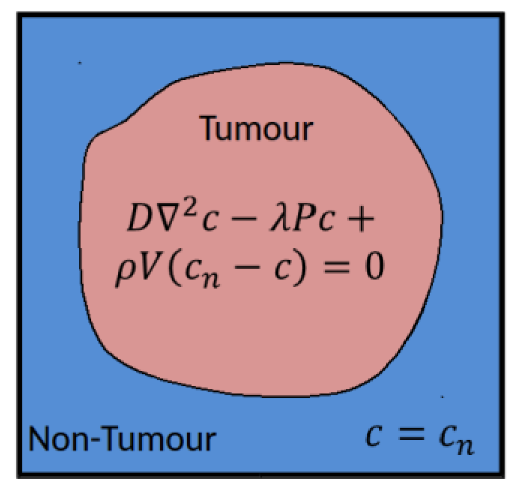
Figure 2.
Multimodeler Hypermodel communication scheme.
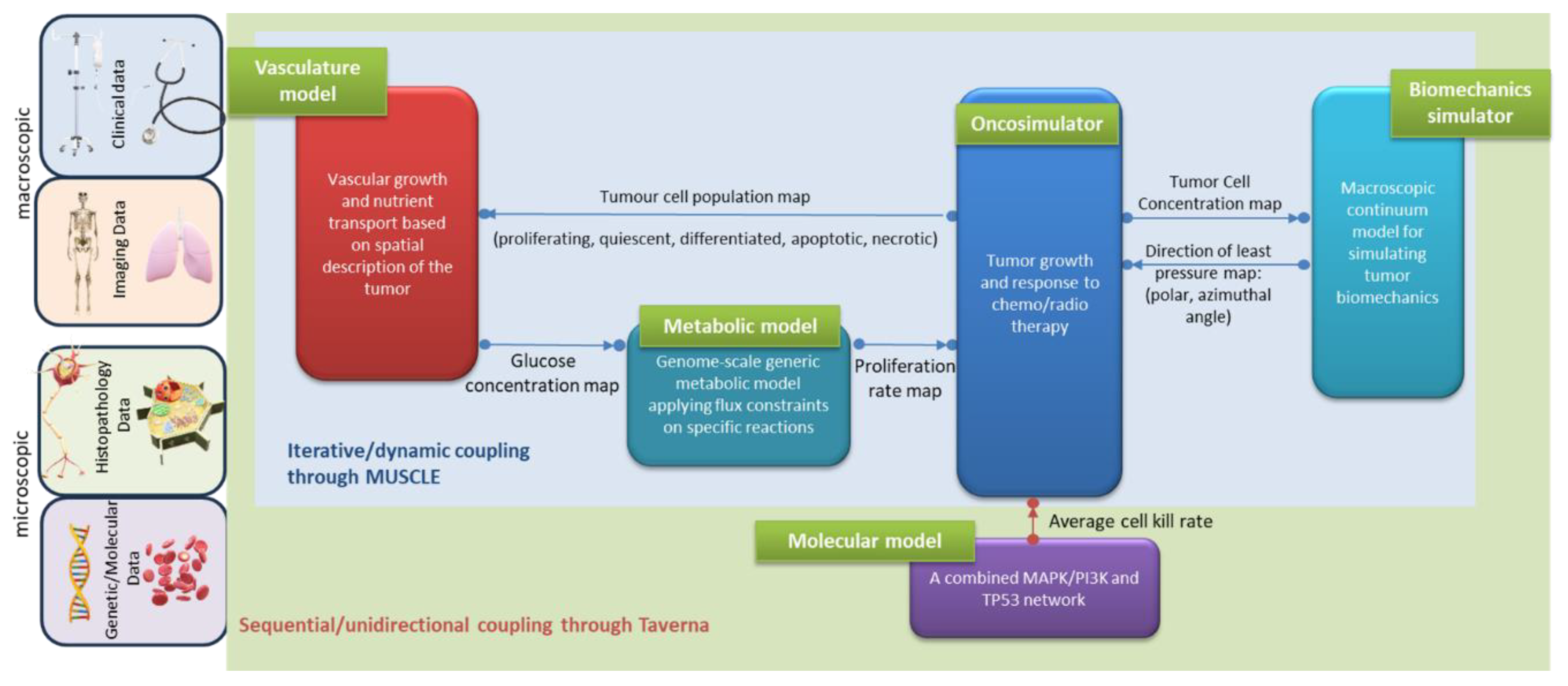
Figure 4.
Predicted linking variables between the metabolic model and the HDC tumor growth model for specific flux bounds in the corresponding reactions.
Figure 4.
Predicted linking variables between the metabolic model and the HDC tumor growth model for specific flux bounds in the corresponding reactions.
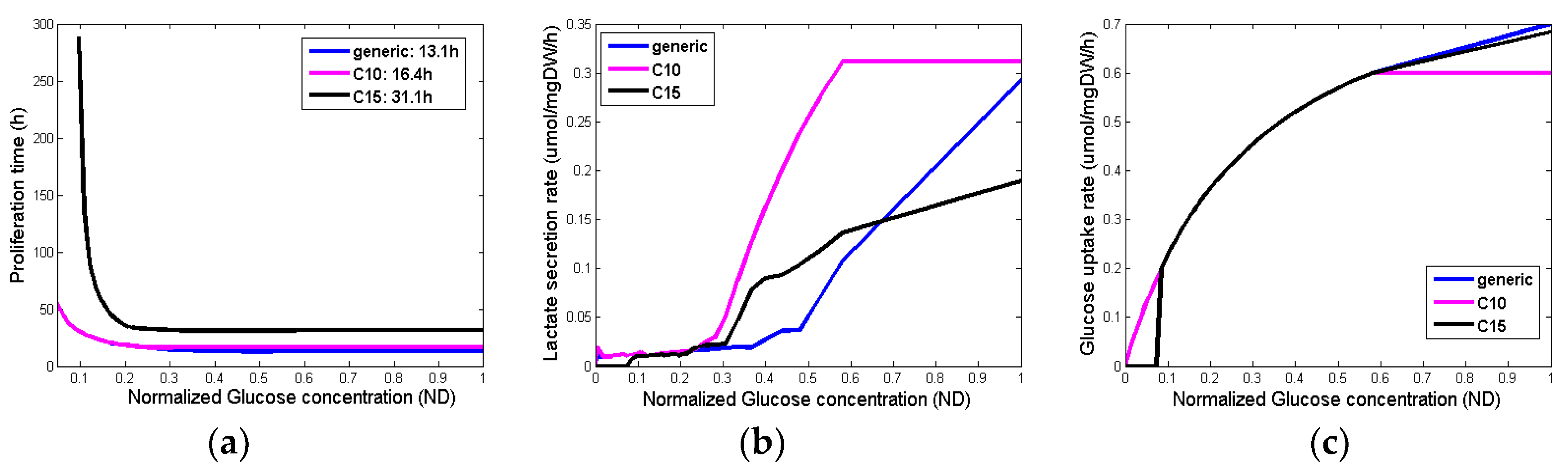
Figure 5.
Personalised FEM model for WT scenario, derived from patient anatomy.
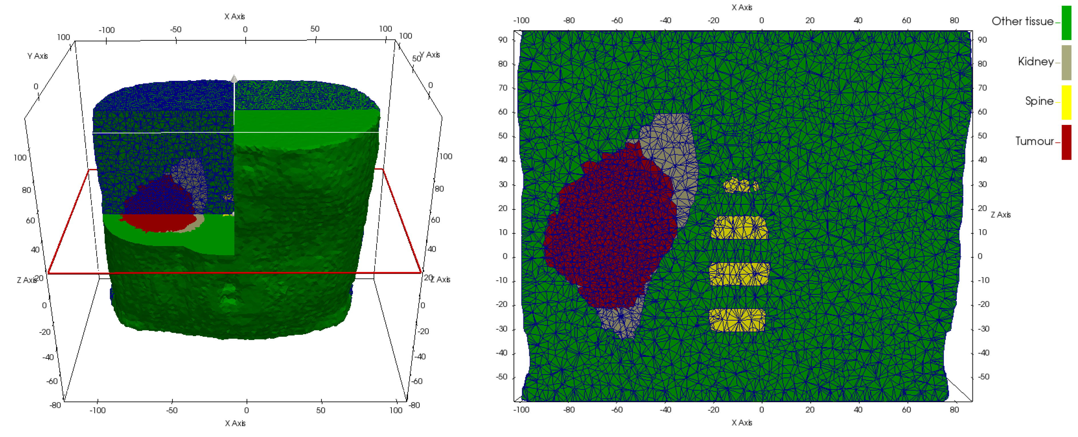
Figure 6.
Personalized FEM model for NSCLC scenario, derived from patient anatomy.
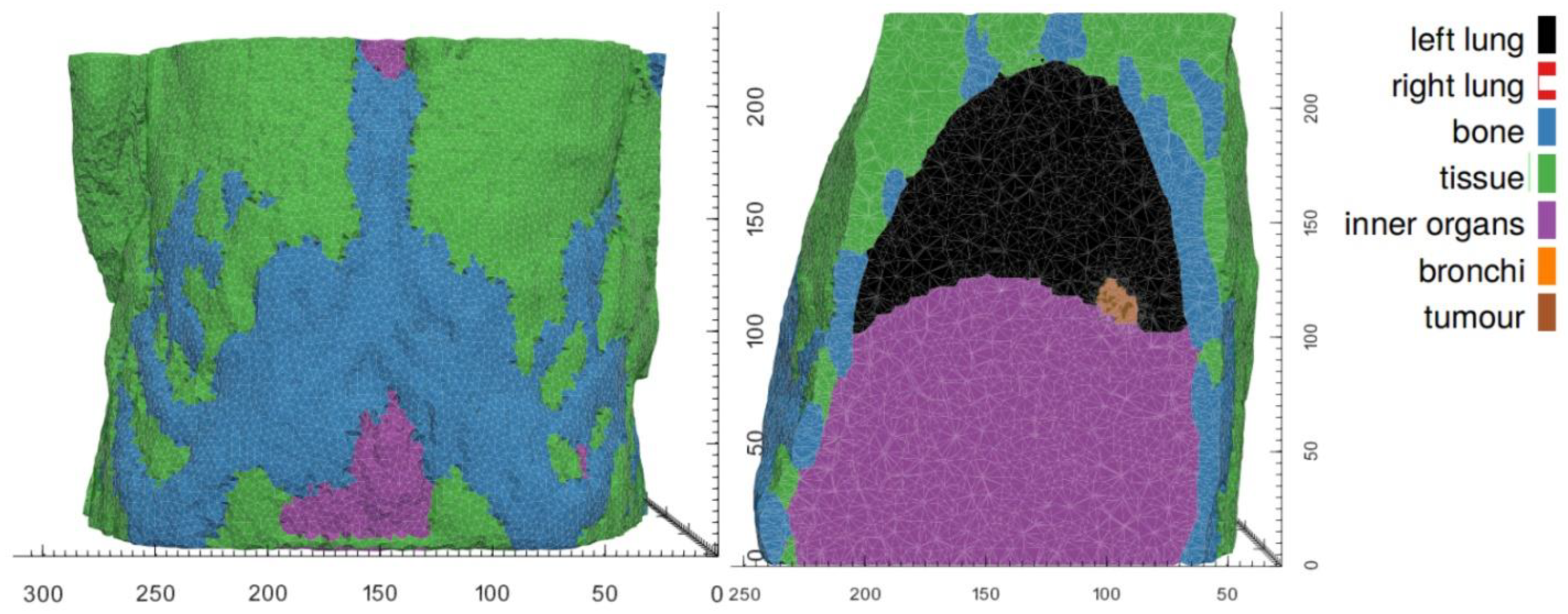
Figure 8.
Box-and-whisker plots of the predicted volume one year post radiotherapy and the estimated TCP for a NSCLC case. Scenario 1 considers the applied therapeutic scheme and dosage. Scenario 2 assumes a reduced administration dose. Scenario 3 assumes that radiotherapy is administrated one month earlier.
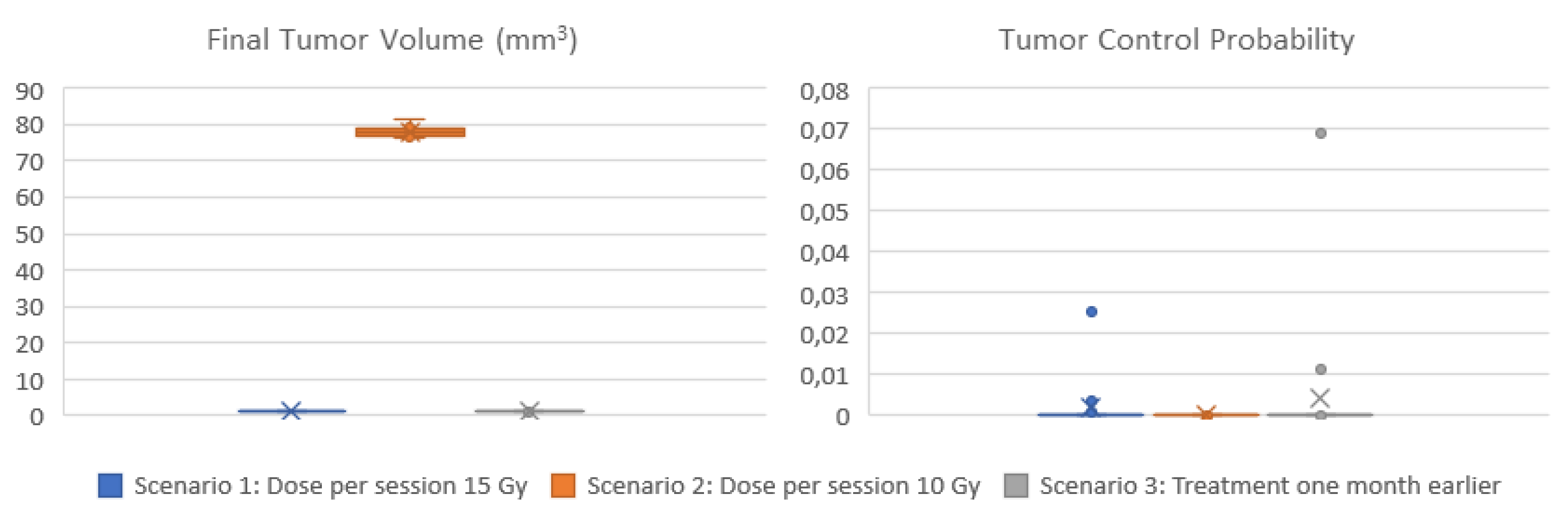
Figure 9.
Box-and-whisker plots of the predicted volume reductions at the time of 2nd image acquisition for two WT patients. Black dashed line corresponds to real volume reduction. 9 proliferation profiles, i.e., combinations of (Td, GF), and 3 cell proliferation times have been considered. Based on metabolic model the cell proliferation time of WT cancer cells can vary between approximately 13 and 50 hr depending on glucose concentration (Figure 4). Panels (a) and (d) correspond to an adequate glucose concentration and a low cell proliferation time=13hr. Panels (b) and (e) correspond to a moderate glucose concentration and a cell proliferation time=30hr. Panels (c) and (f) correspond to a low glucose concentration and a cell proliferation time =50hr.
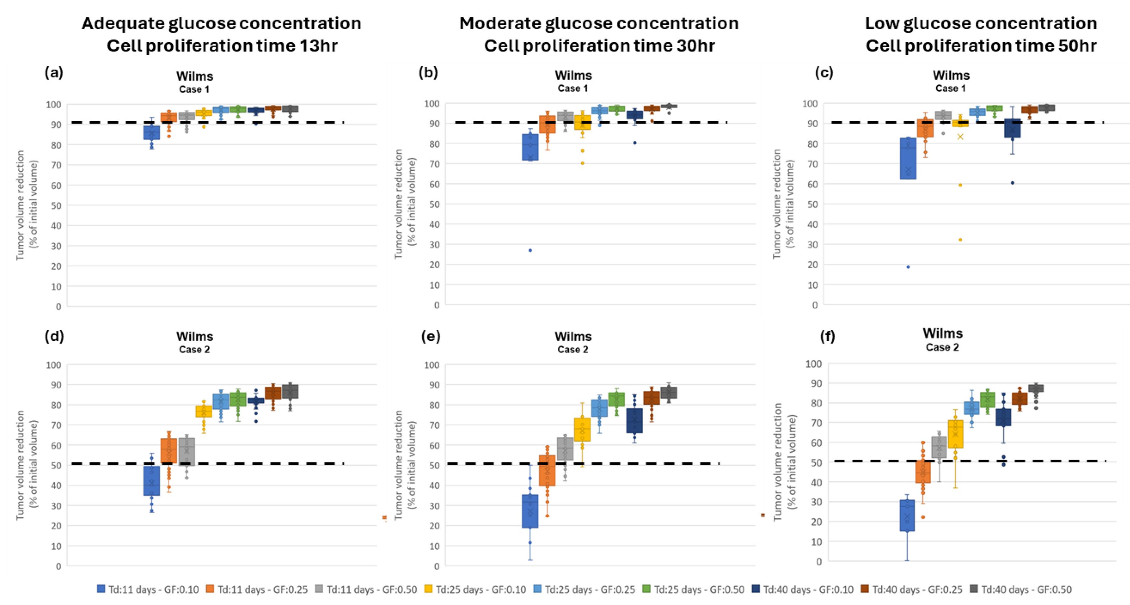
Figure 7.
Visual comparison of shape and position between simulated (red) and observed (blue) tumors at the respective second imaging time point (t2). In the NSCLC scenario, during the simulation period (day 1-98), the tumor volume increases (simulation of free growth before start of irradiation). In the WT scenarios, the tumors decreases (simulation of tumor response to chemotherapy) during the simulation periods (case 1: day 0-41; case 2: day 0-28).
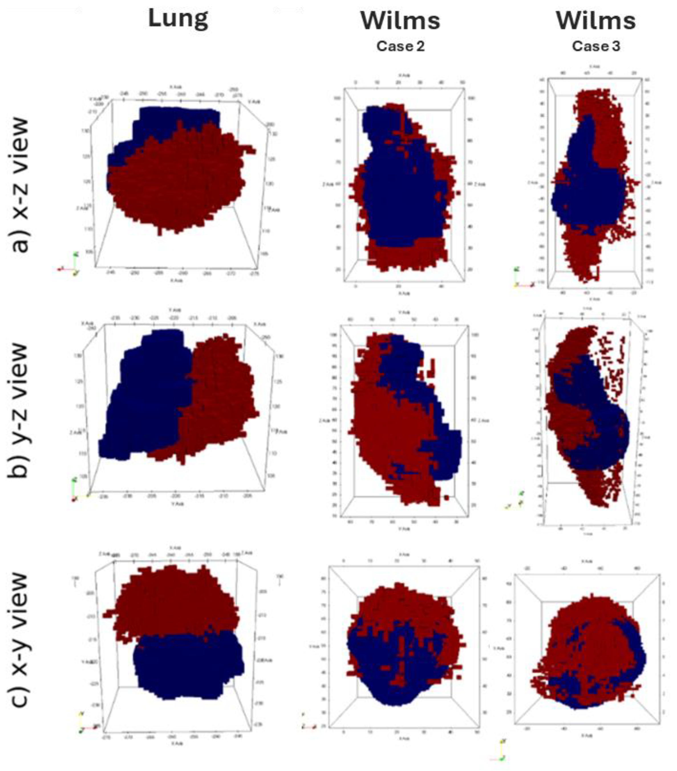
Table 2.
Specific metabolism proteome clusters upregulated in lung cancer as reported in [37].
Table 2.
Specific metabolism proteome clusters upregulated in lung cancer as reported in [37].
| Cluster ID | Cluster proteins (gene names) | Excluded from model |
|---|---|---|
| C10 | ADSS, ATP2A2, CTPS1, IMPDH2, PKM2, PTGES3, SGPL1 | SGPL1 |
| C15 | NAT10, NME2, OAT, PPAT, SHMT2, GART, PAICS, SRM, UMPS, QARS, ABCE1, ABCF2, ACOT7 |
OAT, SHMT2 |
Table 3.
Assumed parameter values for the vasculature hypomodel for WT and NSCLC.
| Symbol | Description | Unit | Value | Source |
|---|---|---|---|---|
| Glucose Diffusivity | mm2.hr-1 | 0.396 | [39] | |
| Glucose Consumption Rate | (Num cells)-1.hr-1 | 7.6e-10 | Modified from [39] | |
| Glucose Concentration in Non Tumor Regions | Kg.m3 | 0.9 | Value used in metabolic hypomodel | |
| Vascular Delivery Efficiency | hr-1 | 0.25 | User chosen/fit to data |
Table 4.
Tissues and mechanical tissue parameters for WT and NSCLC scenarios.
| Tissue Type | E [Pa] | Poisson ratio |
|---|---|---|
| WT scenario | ||
| Healthy kidney | 5.3 ∙ 103 | 0.40 |
| Bone | 1.0 ∙ 109 | 0.30 |
| Other tissues | 5.0 ∙ 103 | 0.40 |
| Tumor | 20.0 ∙ 103 | 0.40 |
| NSCLC scenario | ||
| Lung tissue | 5.0 ∙ 103 | 0.40 |
| Bone | 1.0 ∙ 109 | 0.30 |
| Other tissues | 5.0 ∙ 103 | 0.40 |
| Inner organs | 5.0 ∙ 103 | 0.40 |
| Bronchi | 5.0 ∙ 103 | 0.40 |
| Tumor | 10.0 ∙ 103 | 0.40 |
Table 5.
Cell kill rate (i.e., fraction of cells killed) averaged over various growth factor concentration and cell cycle times as obtained from the molecular model compared with the results obtained from the LQ model. Typical radiosensitivity parameters are considered to be α=0.35Gy-1, β=0.035Gy-2 [41]. Values are rounded at the 3rd decimal place.
| Dose per fraction (Gy) | Cell kill rate based on LQ | Modified cell kill rate |
|---|---|---|
| 5 | 0.928 | 0.433 |
| 10 | 0.999 | 0.712 |
| 15 | 1.000 | 0.905 |
| 20 | 1.000 | 0.979 |
Table 6.
Assumed parameter values of the Oncosimulator and tumor characteristics for NSCLC.
| Parameter | Value range | Reference(s) |
|---|---|---|
| Tc (h) | 20-134 | [42,43], the upper limit is constrained by the proliferation rate computed by the metabolic hypomodel |
| TG0 (h) | 96-240 | [44] |
| TN (h) | 1-100 | [45,46], estimation based on the extend of necrosis reported in literature |
| TA (h) | 1-25 | [47,48,49] |
| NLIMP | 13-24 | estimation based on frequency of tumor initiating cells reported in literature |
| RA (h-1) | 0-0.001 | estimation |
| RADiff (h-1) | 0.0001-0.02 | extension of [50,51,52,53] |
| RNDiff (h-1) | - | estimated per virtual tumor based on patient’s data (GF) |
| PG0toG1 | 0-0.2 | |
| Psleep | - | estimated per virtual tumor based on the cell proliferation rate computed by the metabolic hypomodel |
| Psym | <0.3 | [54,55], estimated per virtual tumor based on patient’s data (Td) |
| CKR | Study 1, 3: 0.905 Study 2: 0.712 |
estimated by molecular hypomodel based on patient’s miRNA and mutation data |
| α/β | 4-10 | [56] |
| Cell proliferation rate | 70h | computed by metabolic model |
| Stem/living | 0,00001-0,00025 | [57] |
| GF | 23% | Patient‘s data: Ki-67 |
| Td | 370 days | patient‘s data: tumor volumetric increase between two successive imaging data prior therapy |
| Necrotic/Total | <30% | based on [58,59] |
| Apoptotic/Total | <5% | [60] |
Table 7.
Cell kill rate (CKR) (i.e., fraction of cells killed) averaged over various growth factor concentration and cell cycle times and adjusted to patient specific genetic variation. Typical CKRs are considered to be CKRVincristine=0,28, CKRActinomycin=0.4, CKRcombo=0.568 (Calculated following methodology in supplement S3 from [8] based on data from [63,64]. Values are rounded at the 3rd decimal place.
| Vincristine (mg/m2) | Actinomycin (ug/kg) | Cell-Death-Mean propability | CKR Adjusted | |
|---|---|---|---|---|
| Case 1 | 0 | 0 | 0.179 | N/A |
| 1 | 650 | 0.527 | 0.916 | |
| Case 2 | 0.83 | 0 | 0.112 | 0.28 |
| 0.83 | 540 | 0.149 | 0.673 |
Table 8.
Assumed parameter values for the Oncosimulator for the WT.
| Parameter | Value Range | Reference(s) |
|---|---|---|
| Tc (h) | 11-50 | [63,65,66], constrained by the output of metabolic hypomodel |
| TG0 (h) | 96-240 | [44] |
| TN (h) | 1-200 | [45,46], estimation based on extend of necrosis in resected tumors reported in literature |
| TA (h) | 1-25 | [47,48,49] |
| NLIMP | 13-24 | Estimation based on frequency of tumor initiating cells reported in literature |
| RA (h-1) | 0-0.001 | - |
| RADiff (h-1) | 0-0.02 | - |
| RNDiff (h-1) | - | estimated per virtual tumor based on patient’s data (GF) |
| PG0toG1 | 0-0.2 | |
| Psleep | - | estimated per virtual tumor based on the cell proliferation rate computed by the metabolic hypomodel |
| Psym | - | [54,55], estimated per virtual tumor based on patient’s data (Td) |
| CKR | - | Estimated by molecular hypomodel basen on patient’s miRNA |
| GF | 0-80% | [67,68] |
| Td | 11-40 days | [69] |
| Necrotic/Total | 0-100% | [70] |
Disclaimer/Publisher’s Note: The statements, opinions and data contained in all publications are solely those of the individual author(s) and contributor(s) and not of MDPI and/or the editor(s). MDPI and/or the editor(s) disclaim responsibility for any injury to people or property resulting from any ideas, methods, instructions or products referred to in the content. |
© 2024 by the authors. Licensee MDPI, Basel, Switzerland. This article is an open access article distributed under the terms and conditions of the Creative Commons Attribution (CC BY) license (http://creativecommons.org/licenses/by/4.0/).
Copyright: This open access article is published under a Creative Commons CC BY 4.0 license, which permit the free download, distribution, and reuse, provided that the author and preprint are cited in any reuse.


