
Submitted:
07 March 2024
Posted:
07 March 2024
You are already at the latest version
Abstract
Climate change poses a significant threat to global food security, necessitating a thorough examination across multiple dimensions. Establishing appropriate food security evaluation indicators that align with the evolving concept of food security is imperative. This study enhances food security evaluation by refining a multi-dimensional framework and analyzing the impact of climate change across various regions from 2002 to 2021. By constructing an Food Security Index system composed of a three-tier indicator system and employing the entropy method for weighting, we assess the impacts of climate change on food security using a climate-economic model. Regression analysis reveals a negative linear relationship between mean temperatures and food security (p<0.01), while precipitation impacts food security non-linearly, particularly exhibiting inverse U-shaped patterns in major grain-producing and grain-consuming areas. Extreme high temperatures consistently reduce food security, whereas extreme precipitation displays a complex, statistically significant inverse U-shaped association. In regions where production and consumption are balanced, mean temperatures have a negative effect on food security, while precipitation exhibits a positive correlation, but excessive precipitation can have adverse effects. These findings highlight the intricate interplay between climate change, regional disparities, and food security in China, emphasizing the need to consider multi-dimensional factors and regional variations in addressing food security challenges. These insights are invaluable for policy-making and planning aimed at enhancing food security in China.
Keywords:
Climate change
; Food security
; Economic-climate model
1. Introduction
Climate change poses a great challenge to global food security and current changes in global food insecurity can be plausibly attributed to climate change [1,2]. Numerous studies have discussed the impact of climate change on various aspects of food security, including the quality of agricultural products [3], the impact on prices [4], as well as the impact on agricultural production environments such as farmland [5,6], agricultural water use [7], and agricultural ecosystems [8,9]. In fact, the global food security situation is currently facing unprecedented challenges, with nations experiencing an increase in systemic food security risks [10,11]. According to the 2022 State of Food Security and Nutrition in the World report released by the United Nations Food and Agriculture Organization [12], food security issues still exist widely, especially against the backdrop of changing climates. Climate change and extreme climate events have become one of the main contributors to the worsening of global hunger conditions, seriously affecting all aspects of food security, including food supply, access, utilization, and stability.
As the world’s largest producer and consumer of food, China supports nearly 20% of the global population with only 9% of the world’s cultivated land and 6% of freshwater resources [13,14]. Food security has always been seen as China’s most important issue related to people’s livelihood, as well as a crucial foundation for economic development, social stability, and national security. However, with rising temperatures, frequent extreme weather events, and changes in precipitation patterns, China’s food production and supply chain are facing increasingly severe threats of climate change, bringing more uncertainty risks [15,16,17,18]. The government implements comprehensive strategies to ensure the stability and continuous improvement of food security through technological advancement, land protection, subsidies, food reserves, market regulation, agricultural insurance, and international cooperation. Climate in China typically varies significantly across regions due to its vast land area and diverse climatic. Therefore, understanding the multi-dimensional impacts of climate change on China’s food security is crucial.
The concept of food security has undergone three significant evolutions internationally [19]. In 1974, the Food and Agriculture Organization of the United Nations (FAO) defined food security as "the ability of all people, at all times, to access enough food for an active and healthy life." This definition emphasized quantitative security. In 1983, the definition evolved further to include affordability, emphasizing economic security, particularly for low-income groups. At the 1996 World Food Summit, it raised that "food security exists when all people, at all times, have physical and economic access to sufficient safe and nutritious food that meets their dietary needs and food preferences for an active and healthy life," highlighting nutrition and health. Across the world, there are mainly two authoritative international organizations for food security evaluation are the FAO and the Economist Intelligence Unit (EIU). The FAO’s food security evaluation system mainly focuses on individual nutritional status [12], constructed from four dimensions: food supply level, food availability, food utilization level, and stability. The EIU’s food security index (the Global Food Security Index, GFSI) focuses the categories of affordability, availability, and quality and safety [20], and and it holds global significance as a demonstrative tool.
Food security level is impacted by various natural and human factors, and there are many relevant studies. Study on spatio-temporal evolution and scale differences of food security risk patterns in China [21] have provided a comprehensive analysis of the evolving risk patterns and their implications for policy-making and risk management. Zhang et al. (2022) [22] explored the spatio-temporal evolution and coordination of agricultural green efficiency and food security in China. A quantitative evaluation of future food security risk considering water scarcity as a key factor is conducted [23], which highlighted the importance of water resources in ensuring food security and the need for effective water management strategies. The relationship between gross primary production, solar-induced chlorophyll fluorescence, terrestrial water storage, crop grain production, and agricultural investment and policy are examined [24], providing insights into the complex interactions between these factors and their impact on food security. Focusing on the interaction between food production security and agricultural ecological protection, Liu et al. (2023) [25] emphasized the need for a balanced approach that considers both food production and ecological sustainability. The work on the impact of low-intensity pollution on China’s sustainable development of food security highlighted the role of pollution in compromising food security and the need for effective pollution control measures [26]. Yang and Cui (2023) [27] discussed the balance between feed grain security and meat security, examining the trade-offs and synergies between the two. Zhang et al. (2023) [28] assessed the impacts of global climate change on water and food security in the black soil region of Northeast China using an improved SWAT-CO2 model. Their findings provided insights into the potential impacts of climate change on water resources and food production in this region, highlighting the need for adaptive measures to mitigate these impacts.
Based on this, it is crucial for assessing global and regional food security to establish appropriate food security evaluation indicators. Heady and Ecker (2013) [29] suggested concentrating on four key indicators: calories, poverty, dietary diversity, and subjective indicators. In contrast, Coates (2013) [30] advocated for the utilization of five dimensions: food sufficiency, nutrient adequacy, cultural acceptability, safety, and certainty and stability. Domestic scholars have constructed food security evaluation systems based on China’s national conditions. These systems have evolved from a single focus on supply-demand balance to emphasizing food availability, especially for low-income groups, and then to focusing on ecological and resource security, as well as dietary nutrition and health. Representative scholars and their research include: Zhang et al. (2015) [31] constructed an indicator system covering eight aspects, including supply, distribution, consumption, utilization efficiency, security outcomes, stability, sustainability, and regulatory capacity. Wang et al. (2022) [32] established a food security evaluation system from the perspective of food security guarantee capabilities, covering five dimensions: basic guarantee capabilities, market regulation capabilities, production supply capabilities, utilization of international market resources, and agricultural modernization development capabilities. Gao and Zhao (2023) [33] proposed strengthening the foundation of food security from multiple aspects such as total quantity security, quality improvement, structural optimization, ecological sustainability, and supply diversification. These studies have provided a useful theoretical foundation for understanding the multi-dimensional impacts of climate change on China’s food security.
Most studies on food security systems primarily focused on grain production, supply and demand, and distribution, with a strong emphasis on quantitative food security. However, as economic and social development progressed, food security was given new connotations and objectives. In the contemporary era, the concept of food security has broadened to encompass not only ensuring production capacity but also promoting nutritional, green, diverse, and open food production. This implies safeguarding both quantitative and qualitative food security while maintaining environmental friendliness, economic efficiency in food production, and high resource utilization efficiency. A recent work by Cui and Nie (2019) [34] proposed a comprehensive food security evaluation system encompassing five dimensions: quantitative security, qualitative security, ecological environmental security, economic security, and resource security. Building upon this framework, the present study has refined and improved the food security evaluation indicator system, aiming to provide a more holistic and comprehensive assessment of food security in the modern context.
Therefore, based on inter-provincial panel data, this study constructs multi-dimensional food security evaluation indicators to explore the mechanism and actual impact of climate change on food security, and analyzes the regional differences in the impact of climate change on food security in different regions. The entropy method is employed to determine the weights of indicators and calculate the for each province in China. A model of economy-climate as the C-D-C model [35,36] is introduced to assess the multi-dimensional impacts of climate change on China’s food security. This work will complement the existing evidence of factors influencing food security, help the Chinese government formulate more comprehensive and targeted policies and measures, provide useful policy insights for addressing the complex challenges of climate change to China’s food security, and ensure the sustainability and safety of China’s food supply.
2. Materials and Methods
2.1. Climate Data Source
The climate data used in this study come from the CN05.1 gridded observation dataset developed and released by the China’s National Climate Center [37]. This dataset is based on daily observation data from more than 2,400 national stations (basic, benchmark, and general stations) of the National Meteorological Information Center. The variables included are: daily mean temperature, precipitation, maximum temperature, minimum temperature, mean wind speed, relative humidity, and evaporation. In this study, the annual average temperature, annual precipitation, accumulated temperature above C (Tm10), extreme high temperature index (TX90p, Percentage of days when daily maximum temperature percentile) , and extreme precipitation index (R95TOT: Accumulation of summer precipitation when daily precipitation percentile) are calculated using these variables.
2.2. Agricultural Data Source and China’s Grain Regional Division
The provincial agricultural data utilized in this study consist of two main components. Firstly, the construction of food security index data encompasses various metrics, including grain production volatility, grain yield per unit area, per capita grain production, pesticide and fertilizer usage per unit of cultivated land area, proportion of grain affected by disasters, grain consumer price index, Engel’s coefficient for rural residents, cultivated land area per unit of grain production, and water resources used per unit of grain production. Secondly, agricultural input data comprises planted area, effective irrigation area, total agricultural machinery power. These datasets are sourced from multiple authorities such as the National Bureau of Statistics, provincial statistics bureaus, the China Economic Data website, the National Intellectual Property Administration, the "China Statistical Yearbook," the "China Rural Statistical Yearbook," and provincial statistical yearbooks, primarily accessed through the publicly available website https://data.stats.gov.cn/. Owing to data unavailability and to ensure research feasibility, data from the Hong Kong, Macau, and Taiwan regions were excluded from this study.
According to China’s grain regional division, 31 provinces can be divided into three regions, namely, the main grain-production area (MPA), the main grain-consumption area (MCA), and the producing-consumption balance area (BA). The MPA refers to the key grain production areas with geographical, soil, climate, technological, and other advantages, which are suitable for planting certain grain crops and have certain resource advantages, technological advantages, and economic benefits, including 13 provinces (Heilongjiang, Jilin, Liaoning, Neimenggu, Hebei, Henan, Shandong, Jiangsu, Anhui, Jiangxi, Hubei, Hunan, and Sichuan). The MCA refers to the grain consumption area with relatively developed economy, but with a large population and limited land resources, low self-sufficiency rate of grain, and a large gap between grain production and demand. It is mainly concentrated in the southeastern coastal areas and big cities, including 7 provinces (Beijing, Tianjin, Shanghai, Zhejiang, Fujian, Guangdong, and Hainan). The BA refers to the provinces that contribute limitedly to the national grain production but can basically maintain self-sufficiency, including 11 provinces (Shanxi, Ningxia, Qinghai, Gansu, Xizang, Yunnan, Guizhou, Chongqing, Guangxi, Shaanxi, and Xinjiang).
2.3. The Establishment of Food Security Indicator System
When measuring the food security level of each province in China, the entropy method is used to determine the weights of the three-level indicators of the food security evaluation indicator system as is shown in Table 1, and the food security index of each province is calculated accordingly.
2.3.1. Detailed Explanation of the Indicators
Firstly, the Quantitative Security (s1) solves the problem of whether people can "eat enough", directly reflecting the level of grain supply. It is the foundation and most important indicator of food security. In this work, three indicators are selected as follows, both of which are positive indicators:
- Grain Production Fluctuation Rate (%) . It refers to the measure of changes in grain production over a specific period of time indicating the stability or variability of grain production from year to year.
- Grain Yield per Unit Area (kg/hectare). It measures the grain production efficiency of a region.
- Per Capita Grain Production (kg). It refers to the average amount of grain produced per person in a given region or country.
Secondly, Qualitative Security (s2) measures the issue of whether people can "eat safely and healthily". This article selects two indicators, both negative, as follows:
- Pesticide Usage per Unit of Cultivated Area (kg/hectare). It measures the amount of pesticide applied to a specific area of landr reflecting the intensity of pesticide applications.
- Fertilizer Usage per Unit of Cultivated Area (Pure Quantity, kg/hectare). It refers to the quantity of fertilizers applied to a specific land area. Fertilizer is known as the "food" of grain, mainly used to improve soil fertility and land yield per unit area. However, excessive application of fertilizer leads to a decrease in soil organic matter, soil hardening, a decrease in land quality, and pollution of irrigation water.
Thirdly, Ecological Environment Security (s3) examines the sustainability of food production. Food production should not only consider whether the current food production and quality can meet the needs of contemporary people, but also investigate the sustainability of resources. The Grain Disaster Rate is selected as follows:
- Grain Disaster Rate (%). It measures the impact and response capabilities of each province to diseases, pests, and climate disasters through the proportion of food crops affected by disasters.Table 1. Food Security Indicator System involved in this study.
Tier 1 Indicator Tier 2 Indicator Tier 3 Indicator Indicator Direction* Food Security Index
(FSI)Quantitative Security
(s1)j1: Grain Production Fluctuation Rate (%) Positive j2: Grain Yield per Unit Area (kg/hectare) Positive j3: Per Capita Grain Production (kg) Positive Qualitative Security (s2) j4: Pesticide Usage per Unit of Cultivated Area (kg/hectare) Negative j5: Fertilizer Usage per Unit of Cultivated Area (Pure Quantity, kg/hectare) Negative Ecological Environment
Security (s3)j6: Grain Disaster Rate (%) Negative Economic Security
(s4)j7: Consumer Price Index for Grain Products (Previous Year = 100) Negative j8: Rural Residents’ Engel Coefficient (%) Negative Resource Security
(s5)j9: Cultivated Area Used per Unit of Grain Production (hectare/ton) Negative j10: Water Resources Used per Unit of Grain Production (cubic meters/ton) Negative * "Positive" indicates that a higher numerical value of the indicator corresponds to a higher level of food security; "Negative" indicates that a lower numerical value of the indicator corresponds to a higher level of food security.

Then, Economic Security (s4) measures whether people can "afford" to eat. This work selects two negative indicators as follows:
- Consumer Price Index for Grain Products (Previous Year = 100). It is a measure that tracks changes in the prices of grain-related products consumed by the general population.
- Rural Residents’ Engel Coefficient (%). It refers to the proportion of food expenditure in the total consumption expenditure of rural households. This coefficient provides insights into the living standards and consumption patterns of rural residents.
Lastly, Resource Security (s5) examines the resource occupation of food production. This article selects two negative indicators as follows:
- Cultivated Area Used per Unit of Grain Production (hectare/ton). It refers to the amount of land required to produce a certain quantity of grain. It is a measure that indicates the efficiency of land use in grain production.
- Water Resources Used per Unit of Grain Production (cubic meters/ton). It refers to the amount of water consumed in the production of a specific quantity of grain. This metric is crucial in assessing the water efficiency of agricultural systems and the sustainability of grain production practices.
2.3.2. The Entropy Weight Method
The entropy weight method is a commonly used approach for evaluating the effectiveness of multiple attributes or criteria in decision-making problems. It is based on the concept of entropy from information theory, which measures the uncertainty or the amount of information contained in a random variable or a set of data. In the entropy weight method, the entropy value of each evaluation criterion is calculated. This entropy value reflects the degree of dispersion or uncertainty associated with the data for that criterion. The weights of the criteria are then determined based on their entropy values. Criteria with higher entropy values (indicating greater uncertainty or dispersion) are assigned lower weights, while criteria with lower entropy values (indicating less uncertainty or dispersion) are assigned higher weights. The method provides a quantitative measure of the contribution of each criterion to the overall decision result. It is often used in multi-attribute decision-making problems where there are multiple criteria or indicators that need to be considered simultaneously.
In this work, the entropy weight method the entropy weight method is performed to determine the weight of each indicators in the Food Security Indicator System in Table 1. Detailed steps of how to perform this method can be seen in section Appendix A.1.
2.4. The Panel Data Analysis Method
Panel Data Analysis is a statistical technique used to analyze data that combines both cross-sectional and time-series dimensions. This type of data, often referred to as "panel data" or "longitudinal data," involves observations of multiple entities across multiple time periods. It can be used to estimate the effects of time-invariant and time-varying explanatory variables on a dependent variable, taking into account both the cross-sectional and time-series dimensions of the data. The analysis typically involves fitting a regression model to the panel data, where the dependent variable is regressed on a set of explanatory variables. Panel regression analysis has a wide range of applications in various fields, including economics, finance, sociology, and political science. It is particularly useful when studying processes that involve both individual and time-varying factors, such as economic growth, firm performance, or social change.
In this work, a climate-economic model is used to assess the multi-dimensional impacts of climate change on China’s food security. The establishment of this model can be seen in section Appendix A.2.
3. Results
3.1. Climate Mean State and Variability
Agriculture is deeply intertwined with climate. Climate conditions, such as temperature, rainfall, and humidity, significantly impact crop growth, yield, and diversity. Adapting agricultural practices to specific climates is crucial for sustainable food production. Thus, the basic conditions of climate and its changes are presented. Surface air temperature and precipitation over China for the period of 2002-2021 are derived from the CN05.1 observational dataset, as is shown in Figure 1.
For the 20-year mean annual averaged temperature in Figure 1a, it shows that temperature in China typically varies significantly across regions due to its vast land area and diverse climatic zones. However, in general, the average annual temperature in China ranges between C to C, with a mean of around C to C. The northern regions, including the Northeast, North, and parts of the Northwest, generally have cooler annual temperatures, averaging around C to C. These areas experience colder winters and relatively warmer summers. The central and southern regions, including the East, Central, South, and Southwest, have warmer annual temperatures, averaging between C to C. The mountainous regions, such as the Himalayas in the west and the Qinghai-Tibet Plateau in the northwest, have significantly lower annual temperatures, often below 0°C due to their high altitude. In Figure 1b, it shows that the most pronounced year-to-year variations occur in the North and Northeast regions. Along with the global warming, China has seen a general trend of warming over the past 20 years, with average annual temperatures increasing slightly, as is shown in Figure 1c. However, this trend is not uniform across the country. Some regions, especially in the north, central and southwest parts, have experienced more pronounced warming than other regions, with linear trends larger than C per 10 years.
Climatological mean precipitation are presented in Figure 1d, generally showing that the southern regions of China receive higher average annual precipitation than the northern regions. The southern areas, including the South, East, and parts of the Central and Southwest regions, experience abundant rainfall with higher than 1000 mm per year. These regions are influenced by the East Asian monsoon, which brings moist air from the oceans, resulting in frequent rainy seasons and abundant precipitation. By contrast, the northern regions, including the North, Northwest, and parts of the Northeast, receive lower average annual precipitation, ranging from 200 to 600 mm per year. These areas have a more continental climate, with dry winters and limited moisture supply, leading to lower precipitation levels. Figure 1e shows that the year-to-year variations have similar pattern to the mean precipitation, and the most pronounced variations occur over southeast part. Linear trends of precipitation in Figure 1f shows that regions of Sichuan-Chongqing-Guizhou, Jiangsu-Zhejiang-Shanghai-Anhui, and parts of the Northeast regions have experienced significant increase in annual precipitation, while regions of Eastern Guangdong and Western Guangdong, Henan, Yunnan have experienced decrease in annual precipitation, resulting higher risks of drought in these regions.
3.2. Food Security Evaluation
To more accurately assess the impact of climate change on China’s food security, we should establish an indicator system that can reflect the level of food security. Basing on the indicator system shown in Table 1, the entropy weight method is performed to determine the weight of each indicators in the subsystem. Detailed steps of how to perform this method can be seen in section Appendix A.1. Using provincial panel data collected from public dataset, the food security index (FSI) are derived, together with score series of the five Tier-2 indicators of Quantitative Security (s1), Qualitative Security (s2), Ecological Environment Security (s3), Economic Security (s4), and Resource Security (s5). The respective weights assigned to each individual indicator within the Food Security Indicator System are presented in Table 2. Utilizing the available provincial panel data and the food security indicator system outlined in Table 1, it becomes apparent that Quantitative Security (s1) holds a substantial weight of approximately 63% in determining the overall FSI. This significant influence primarily originates from the key indicator of j3: Per Capita Grain Production (kg). Following closely is Qualitative Security (s2) with a weight of around 13%, while Economic Security (s4) and Resource Security (s5) contribute with weights of approximately 11% and 9%, respectively. Lastly, Ecological Environment Security (s3) accounts for the least, weighing in at around 4%. This distribution of weights highlights the significant influence of various factors on food security and their relative importance within the indicator system.
The fluctuations in the national FSI and its associated indicators are depicted in Figure 2. From a holistic perspective, China’s food security exhibited a fluctuating upward trend over this period as per the FSI. To delve deeper, the Tier-2 indicators in Table 1, which compose the FSI, provide further insights into these variations. Specifically, the Quantitative Security (s1), Ecological Environment Security (s3), Economic Security (s4), and Resource Security (s5) – contributing 62.9%, 3.8%, 10.8%, and 9.4% to the FSI respectively – all exhibit strong positive correlations with the FSI (correlation coefficients of 0.98, 0.94, 0.94, and 0.93 respectively, all exceeding the 99% confidence level), reflecting a similarly fluctuating growth pattern during the specified period. In contrast, the Qualitative Security (s2) demonstrates a negative correlation (-0.62, surpassing the 99% confidence threshold), suggesting a declining trend throughout the same period.
Similar work is conducted by combining panel data on food security indicators in 31 provincial administrative regions of China. Figure 3 introduces the boxplot to show the diversity of on spacial and temporal dimensions. On spacial dimension, as is shown in Figure 3a, five provinces (Heilongjiang, Jilin, Neimenggu, Liaoning, Xinjiang) see higher level of food security, with median values above 0.50. The lowest level of food security occur at Hainan province, with the median value less than 0.30. In terms of mean scores, the top 13 provinces are all in the set of MPA, which is consistent with the national grain production regional division. The 14th to 25th places include 11 provinces, in which 6 provinces (Xinjiang, Chongqing, Yunnan, Guangxi, Shanxi, Ningxia) are BA areas, and 5 provinces (Shanghai, Zhejiang, Tianjin, Beijing, Guangdong) are MCA areas. The remaining 7 provinces with the lowest average grain scores are Fujian, Shaanxi, Guizhou, Xizang, Gansu, Hainan, and Qinghai. Among them, 5 provinces (Shaanxi, Guizhou, Tibet, Gansu, Qinghai) are BA areas, and 2 provinces (Fujian, Hainan) are MCA areas. It can be seen that the food security of the BA areas has already been suffering a warning issued for food security. From a temporal perspective, as is shown in Figure 3b, the provincial food security level generally shows a continuous upward trend. The median value of the 31 provinces has risen from below 0.4 to nearly 0.5.
To quantitatively evaluate the provincial food security level, a Taylor diagram is introduced in Figure 4, which can provide a visual framework for comparing provincial to national wide mean . The radial distance from the origin represents the fraction of provincial variations and national wide mean variation. The temporal correlation coefficient between the provincial and national wide mean is denoted by the angular distance from the x-axis. As can be seen from this figure, there are significant regional differences in food security indices among provinces nationwide. From the perspective of variance, compared to the national wide mean , the standard deviation of for most provinces falls within the range of 0.5 to 1.5. There are four provinces (Heilongjiang, Neimenggu, Jilin, Xinjiang) with standard deviations above 1.5, indicating larger interannual fluctuations. On the other hand, three provinces (Fujian, Guangdong, Zhejiang) have standard deviations below 0.5, indicating smaller interannual variations in their . From the perspective of correlation, the interannual variations of the majority of provinces are relatively consistent with that of the national wide mean . There are 28 provinces with correlation coefficients exceeding 0.7, with the highest exceeding 0.99 (Neimenggu). However, there are 3 provinces (Guangdong, Hainan, Beijing) with correlation coefficients below 0.7, indicating that their variations differ significantly from those of other provinces.
3.3. Empirical Analysis of the Impact of Climate Change on China’s Food Security
On the basis of the understanding of China’s climate conditions and changes over the past 20 years, combined with the newly constructed provincial-level food security index in China, this section employs panel regression analysis methods to investigate the multi-dimensional impacts of climate change on China’s food security during the period of 2002-2021.
Climate change is a significant and growing threat to food security, already affecting vulnerable populations across the world [38]. In the context of climate change, both climate extremes and climate mean are important considerations. Climate change is causing shifts in both the mean and extreme values of weather variables. For example, global warming is leading to higher average temperatures and more frequent and intense extreme heat events. Similarly, changes in precipitation patterns are resulting in both wetter and dryer regions, with more intense rainfall events in some areas and decreased rainfall in others. It is important to consider both climate extremes and climate mean when assessing the impacts of climate change and developing adaptation strategies. Understanding how these two aspects of climate are changing can help us prepare for and mitigate the potential negative impacts of climate change on human society and the natural environment. Thus, two groups of climate variables are analyzed respectively.
3.3.1. Impact of Climate Mean State Change on
Climate change refers to long-term shifts in the Earth’s climate system, including temperature, precipitation, wind patterns, and other weather variables. In this work, the variables of accumulated temperature above C () and yearly accumulated precipitation () are used to represent the climate mean state change for the period of 2002-2021, and are designated to be the explanatory variables. The provincial food security index () is designated to be the dependent variable. Besides, the cultivated land area (), the effective irrigation area (), and the total agricultural machinery power () are selected as the control variables. Both entity-specific fixed effects and time fixed effects have been incorporated into the model.
Firstly, employing a panel regression analysis on the provincial dataset, we confined our attention to the linear effects by considering only the first-order terms of the explanatory variables. This was done using the Panel Data Analysis model (Equation A11) detailed in Appendix A.2. The outcomes from this specific analysis are displayed in Table 3. From the presented table, one can discern that for the Food Security Index (), the coefficient of stands at -0.188, a value that is statistically significant at the p<0.01 level. This implies a negative linear relationship between and , suggesting that as rises, there is a corresponding decrease in the . On the contrary, no statistically significant association exists between and . Regarding control variables, both and exert significant positive influences on food security. The model’s R-squared value amounts to 0.758, signifying that our model effectively accounts for 75.8% of the variability in the dependent variable . This is considered a relatively high R-squared value, indicating that our model offers a good fit to the data, with substantial explanatory power regarding fluctuations in China’s provincial food security levels. Regarding the sub-indicators, it is evident that both Quantitative Security (s1) and Economic Security (s4) demonstrate strong correlations with variations in , where the significance level surpasses p<0.01. This signifies a detrimental effect on Quantitative Security but a favorable impact on Economic Security due to changes in . Additionally, Resource Security (s5) exhibits a negatively correlated relationship with at a significant level of p<0.1, suggesting a decrease as increases. However, no statistically significant effects are observed between and Qualitative Security (s2) or Ecological Environment Security (s3).
Subsequently, to account for the non-linear effects of precipitation and temperature on food security, quadratic terms for the explanatory variables and are incorporated into the model. A refined panel regression analysis is performed using a modified version based on Equation A13 detailed in Appendix A.2. Post-regression, individual U-tests were carried out to examine each variable’s non-linearity. The results from this advanced analysis are showcased in Table 4. The findings reveal that while there is no statistically significant U-shaped relationship between and food security, an inverse U-shaped relationship between and food security has been established as significant. This leads to the conclusion that the effect of temperature () on food security is linear, whereas the influence of precipitation () exhibits a nonlinear pattern. Consequently, only the first-order term of temperature is retained in the model, while both the first-order and second-order terms for precipitation are maintained to reflect its nonlinear impact. This indicates that when annual precipitation falls within a certain optimal range, increasing it can indeed contribute positively to ensuring food security. Yet, beyond a particular threshold, any further rise in precipitation will inversely affect food security levels, leading to a decline. This inverse U-shaped relationship between precipitation and food security is consistently mirrored in the Quantitative Security (s1), Ecological Environment Security (s3), and Resource Security (s5) sub-indicators, suggesting that the effects of precipitation on these dimensions follow a similar pattern of initially improving then potentially deteriorating food security conditions under excessive amounts.
3.3.2. Impact of Climate Extremes Change on
Climate extremes refer to the occurrence of unusually high or low values of weather variables, such as temperature, precipitation, that fall outside the range of normal variations expected in a given region. These extreme events can include extreme heat waves, droughts, floods, and other severe weather conditions. Climate extremes can have significant impacts on human health, agriculture, infrastructure, and ecosystems.
In a similar vein to the examination of mean climate state changes ( for precipitation and for temperature), we use two variables that embody climate extremes: , which represents the percentage of days when the daily maximum temperature exceeds the 90th percentile, and , denoting the accumulated precipitation on days where daily precipitation is equal to or above the 95th percentile. These variables encapsulate climate extremes data for the period between 2002 and 2021 and are thus designated as the explanatory variables in our subsequent analysis. The fixed effects configuration, as well as the inclusion of other variables – including the control variables and the constant term – remain consistent across the analyses.
In the context of solely examining the linear effects of the explanatory variables, we utilized the regression model constructed in accordance with Equation A12 detailed in Appendix A.2. The outcomes from this regression analysis are showcased in Table 5. As evidenced by the table, there is a highly statistically significant (p<0.01) negative association between extreme high temperatures () and food security, indicating that an escalation in intense heat occurrences results in a reduction of food security levels. However, no discernible linear correlation exists between extreme precipitation () and food security. Upon closer inspection of the Tier-2 indicators, it becomes apparent that consistently exerts detrimental impacts on Quantitative Security (s1), Ecological Environment Security (s3), and Resource Security (s5). This uniform manifestation of adverse influence suggests that the deleterious effect of extreme heat on food security is channeled through its impact on these specific sub-indicators.
In the context of examining the non-linear effects encapsulated by the quadratic terms of the explanatory variables, we utilized a regression model derived from Equation A14 detailed in Appendix A.2. The results of this analysis are showcased in Table 6. Our research findings reveal that there is no statistically significant non-linear correlation between and overall food security. However, it is noteworthy that the sub-indicators Quantitative Security (s1) and Economic Security (s4) exhibit opposing U-shaped trends. On the other hand, an inverted U-shaped relationship with statistical significance has been observed between and food security, which has successfully undergone validation via the U-test. This particular relationship is primarily underpinned by the inverse U-shape associations existing between and the following Tier-2 indicators: Quantitative Security (s1), Ecological Environment Security (s3), as well as Resource Security (s5).
3.4. Regional Differences in the Impact of Climate Change on
In order to delve deeper into the regional disparities in the effects of climate change on food security, this study introduces three regional dummy variables: is set to 1 for provinces within the MPA region and 0 for those outside it; similarly, assumes a value of 1 for provinces in the BA region and 0 for others, while takes the value 1 for provinces in the MCA region and 0 otherwise. We proceed with a panel regression analysis using provincial panel data based on the Panel Data Analysis model presented in Equation A15 and A16 within Appendix A.2. Throughout all analyses, the fixed effects settings are maintained consistently, as are the inclusion of other variables such as control variables and the constant term. This approach allows us to discern how the impacts of climate change, including climate mean and climate extremes, vary across different regions with respect to food security.
3.4.1. Impacts of Climate Mean State Change
We initially explore the impacts of climate mean state changes, as represented by (mean temperature) and (precipitation). The outcomes from this investigation are presented in Table 7. These results reveal that a significant negative linear relationship between and the Food Security Index () prevails predominantly in the BA region, with a p-value less than 0.05. Moreover, the analysis also shows a positive linear correlation between and , which is statistically significant at the p<0.01 level in the BA region and marginally significant at the p<0.1 level in the MPA region.
In contrast to linear analysis, the investigation incorporates non-linear effects by including quadratic terms of the explanatory variables. Table 8 showcases the outcomes from this non-linear examination. It is noteworthy that no significant non-linear relationship between and the Food Security Index () can be observed across all three designated regions. However, when it comes to precipitation (), a distinct non-linear pattern emerges: there is a statistically significant inverse U-shaped association between and food security in both the MPA and MCA regions. This implies that beyond certain thresholds, an increase in precipitation does not proportionally enhance food security in these areas; instead, it may lead to diminishing returns or even negative impacts on food security.
Similarly, we performed regression analyses on the climate extremes changes, represented by (extreme high temperature) and (extreme precipitation), examining both linear and non-linear effects. The outcomes of these analyses are presented in Table 9 for linear effects and Table 10 for non-linear effects. In terms of extreme temperatures, a consistent negative linear relationship with food security is observed across all three regions, although this correlation reaches statistical significance at the p<0.01 level only within the BA region. On the other hand, the influence of extreme precipitation exhibits an inverse U-shape relation with food security in all three regions. Notably, this non-linear relationship surpasses the p<0.01 significance threshold in both the MPA and MCA regions, indicating that there is a threshold beyond which increased extreme precipitation negatively impacts food security in these areas.
4. Discussion
The assessment of food security in China is a multifaceted and intricate process, heavily influenced by regional disparities and varying policy frameworks. The complexity of the subject has led to the development of distinct indicator systems reflecting individual research priorities, which may yield differing conclusions when evaluating the nation’s food security status. This study presents a holistic framework for food security analysis that encompasses five key dimensions: Quantitative Security, Qualitative Security, Ecological Environmental Security, Economic Security, and Resource Security. This robust structure builds upon and refines existing indicators, aiming to offer a more integrated and thorough understanding of food security in light of current challenges and dynamics.
Quantitative Security accounts for a critical 63% weight within China’s Food Security Index (FSI). Over time, there has been a general strengthening of China’s food security, with strong positive correlations observed for Quantitative, Ecological Environment, Economic, and Resource Security aspects. However, the decline in Qualitative Security, as indicated by its negative correlation, highlights the vital need for persistent improvements in grain production efficiency and strict adherence to cultivated land red line policies. Core strategies include advancing agricultural technologies, judicious land use management, and stringent protection against overexploitation to ensure sustainable food output and resilience to adversities.
A closer examination of Figure 3 reveals that among the 31 provinces studied, five provinces—Shaanxi, Guizhou, Xizang, Gansu, and Qinghai—in balanced production-consumption regions exhibit notably low food security scores, signifying heightened insecurity and significant challenges to national food security. These regions, characterized by less fertile lands and underdeveloped infrastructure, are prime targets for agricultural improvement initiatives. In response to intensifying food security risks in these balance zones, urgent and comprehensive action is required. This involves enhancing agricultural productivity, protecting arable land, augmenting grain reserves, optimizing logistics, establishing robust emergency plans, promoting climate-smart agriculture, encouraging moderate-scale farming, and implementing targeted support measures. These strategic steps are indispensable for maintaining stable grain supplies and reinforcing national food security amidst growing threats from climate change, dwindling land resources, and volatile market conditions.
Climate change, marked by rising temperatures and more frequent extreme heat events, significantly impacts China’s food security landscape. Precipitation influences display a U-shaped pattern, initially benefiting food production until it reaches a point where excessive levels become detrimental. Therefore, local food security strategies must be adapted to address climate change by assessing regional climate risks, diversifying agricultural outputs, optimally allocating water resources, upgrading agricultural facilities, promoting resilient farming practices, bolstering community resilience, and fostering collaboration across stakeholders to enhance adaptive capabilities. Upholding the red line for cultivated land, improving soil quality, and endorsing moderate-scale farming operations are fundamental elements to strengthen the stability and resilience of agricultural production under an evolving climate scenario.
5. Conclusions
To conduct a comprehensive quantitative assessment of China’s food security, this study devised a provincial Food Security Index () system consisting of five secondary indicators and ten tertiary indicators. The entropy method was employed to assign weights and compute the for each province. Leveraging a climate-economic model, the investigation scrutinized the multifaceted impacts of climate change on China’s food security landscape over the 2002-2021 period, culminating in several noteworthy findings.
China’s diverse climates exhibit increasing temperatures and variable precipitation patterns, with the most significant warming trends observed in its northern, central, and southwestern regions. Southern provinces receive higher annual rainfall due to monsoons, whereas interannual fluctuations in southeast regions elevate the likelihood of drought occurrences.
Quantitative Security elements account for a dominant share (63%) within the overall , which has generally exhibited improvement across multiple dimensions, except for Qualitative Security, which experienced a downturn. While provincial food security levels have improved collectively, they are notably under threat in BA designated areas.
Statistical regression analyses uncovered a robust negative linear relationship between accumulated temperatures () and provincial food security, demonstrating statistical significance at p<0.01. Precipitation, conversely, influences food security in a non-linear fashion, manifesting as an inverse U-shaped curve that becomes substantial when surpassing certain thresholds, particularly in MPA and MCA zones.
Extreme high temperatures consistently lower food security across multiple indicators, while no such linear correlation exists for extreme precipitation. However, there’s a statistically significant inverse U-shaped association between extreme precipitation and food security.
In the specific context of the BA region, exert a significantly detrimental effect on food security, contrasting sharply with the positive correlation found between and food security, a relationship that appears more pronounced in BA compared to MPA. Further, non-linear analyses divulge that beyond certain thresholds, escalating precipitation can lead to diminishing returns or even adverse effects on food security.
Author Contributions
Conceptualization, H.Z. and N.C.; methodology, H.Z.; software, H.Z. and N.C.; validation, N.C., L.Y. and J.X.; formal analysis, H.Z.; investigation, N.C.; resources, H.Z. and N.C.; data curation, H.Z. and N.C.; writing—original draft preparation, H.Z. and N.C.; writing—review and editing, N.C., L.Y. and J.X.; visualization, H.Z. and N.C.; supervision, L.Y.; project administration, J.X.; funding acquisition, L.Y. and J.X. All authors have read and agreed to the published version of the manuscript.
Funding
This research was funded by the National Natural Science Foundation of China (grant number 72293604) and the Shenzhen Science and Technology Program (grant number JCYJ20210324131810029). This work is part of the project conducted by H.Z. for her Master’s degree.
Institutional Review Board Statement
Not applicable.
Informed Consent Statement
Not applicable.
Data Availability Statement
Data are available from the authors upon request.
Acknowledgments
The National Climate Center, the National Bureau of Statistics and other relevant institutes are acknowledged for kindly making their dataset publicly available.
Conflicts of Interest
The authors declare no conflicts of interest.
Abbreviations
The following abbreviations are used in this manuscript:
| Food security index | |
| Accumulated temperature above C | |
| Precipitation, | |
| Percentage of days when daily maximum temperature percentile | |
| Accumulation of precipitation when daily precipitation percentile | |
| FE | Fixed effects |
| Cultivated land area | |
| Effective irrigation area | |
| Total agricultural machinery power | |
| MPA | Main grain-production areas |
| BA | Production-consumption balance areas |
| MCA | Main grain-consumption areas |
Appendix A. Supplement Materials for the Methods
Appendix A.1. Performing the Entropy Weight Method to Composite FSI
The use of entropy weight method to determine the weights of indicators and to composite the follow seven steps:
Step1: Given n samples and m indicators, represents the numerical value of the jth indicator for the ith sample (where i=1, 2, ..., n; j=1, 2, ..., m).
Step2: Indicator standardization: Since the units, dimensions, and scales of the indicators may vary, standardization of the initial indicators is necessary to avoid meaningless values. The following processing methods are applied for positive (eq.A1) and negative (eq.A2) indicators respectively:
Step3: Calculating the proportion of indicator values for the ith sample and jth indicator:
Step4: Obtaining the information entropy of the jth indicator:
Step5: Calculating the redundancy of information entropy:
Step6: Calculating the weights of the indicators:
Step7: Calculating the food security index of the ith sample for each subsystem:
In these formulas used in this work, n represents the number of years, and m represents the number of indicators in the subsystem.
Appendix A.2. The Panel Data Analysis Model
The Cobb-Douglas production function is based on the empirical study of the American manufacturing industry made by Paul H. Douglas and C.W. Cobb. It is a linear homogeneous production function of degree one which takes into account two inputs, labour (L) and capital (C), for the entire output of the manufacturing industry (Q):
On this basis, previous works [35,36] developed a C-D-C model to estimate China’s climate change risks on food production by introducing the impact of climate change:
The formula can be linearized by taking the logarithm:
In this work, climate variables of , , , are used to represent the climate risks on the . Thus, this work developed a formula to determine when considering mean climate change:
in which the the cultivated land area (), the effective irrigation area (), and the total agricultural machinery power () are selected as the control variables. When considering extreme climate change, the formula can be expressed as:
Further, by taking into account the non-linear effects of precipitation and temperature on food production, the quadratic terms for climate variables are introduced into this model as:
and,
To further consider the regional differences in the impact of climate change on food security, this study has set up three regional dummy variables: the MPA region =1 with other regions =0, the BA region =1 with other regions =0, and the MCA region =1 with other regions =0. The relevant formula is as follows (, represent the , and , respectively):
and,
In these formulas, the , and represent regional fixed effects, temporal fixed effects, and random disturbances respectively. Other variables are consistent with the definition in above text as well as in the section of Abbreviations.
References
- Ray, D.K.; West, P.C.; Clark, M.; Gerber, J.S.; Prishchepov, A.V.; Chatterjee, S. Climate change has likely already affected global food production. PLOS ONE 2019, 14, e0217148. [Google Scholar] [CrossRef] [PubMed]
- Dasgupta, S.; Robinson, E.J.Z. Attributing changes in food insecurity to a changing climate. Scientific Reports 2022, 12, 4709. [Google Scholar] [CrossRef] [PubMed]
- Myers, S.S.; Zanobetti, A.; Kloog, I.; Huybers, P.; Leakey, A.D.B.; Bloom, A.J.; Carlisle, E.; Dietterich, L.H.; Fitzgerald, G.; Hasegawa, T.; et al. Increasing CO2 threatens human nutrition. Nature 2014, 510, 139–142. [Google Scholar] [CrossRef] [PubMed]
- Nelson, G.C.; Rosegrant, M.W.; Palazzo, A.; Gray, I.; Ingersoll, C.; Robertson, R.D.; Tokgoz, S.; Zhu, T.; Sulser, T.B.; Ringler, C.; et al. Food security, farming, and climate change to 2050: Scenarios, results, policy options. Report, 2010. [CrossRef]
- Zaveri, E.; Russ, J.; Damania, R. Rainfall anomalies are a significant driver of cropland expansion. Proceedings of the National Academy of Sciences 2020, 117, 10225–10233. [Google Scholar] [CrossRef] [PubMed]
- Cordovil, C.M.d.S.; Bittman, S.; Brito, L.M.; Goss, M.J.; Hunt, D.; Serra, J.; Gourley, C.; Aarons, S.; Skiba, U.; Amon, B.; et al. , Chapter 22 - Climate-resilient and smart agricultural management tools to cope with climate change-induced soil quality decline. In Climate Change and Soil Interactions; Prasad, M.N.V.; Pietrzykowski, M., Eds.; Elsevier, 2020; pp. 613–662. [CrossRef]
- Rosa, L.; Chiarelli, D.D.; Rulli, M.C.; Dell’Angelo, J.; D’Odorico, P. Global agricultural economic water scarcity. Science Advances 2020, 6, eaaz6031. [Google Scholar] [CrossRef] [PubMed]
- Bebber, D.P.; Ramotowski, M.A.T.; Gurr, S.J. Crop pests and pathogens move polewards in a warming world. Nature Climate Change 2013, 3, 985–988. [Google Scholar] [CrossRef]
- Saccone, D.; Vallino, E. Food security in the age of sustainable development: Exploring the synergies between the SDGs. World Development 2022. [Google Scholar] [CrossRef]
- Puma, M.J.; Bose, S.; Chon, S.Y.; Cook, B.I. Assessing the evolving fragility of the global food system. Environmental Research Letters 2015, 10, 024007. [Google Scholar] [CrossRef]
- Sartori, M.; Schiavo, S. Connected we stand: A network perspective on trade and global food security. Food Policy 2015, 57, 114–127. [Google Scholar] [CrossRef]
- FAO.; IFAD.; UNICEF.; WFP.; WHO. The State of Food Security and Nutrition in the World 2022. Repurposing food and agricultural policies to make healthy diets more affordable. Report, 2022. [CrossRef]
- Fan, M.; Shen, J.; Yuan, L.; Jiang, R.; Chen, X.; Davies, W.J.; Zhang, F. Improving crop productivity and resource use efficiency to ensure food security and environmental quality in China. Journal of Experimental Botany 2012, 63, 13–24. [Google Scholar] [CrossRef]
- Qiao, L.; Wang, X.; Smith, P.; Fan, J.; Lu, Y.; Emmett, B.; Li, R.; Dorling, S.; Chen, H.; Liu, S.; et al. Soil quality both increases crop production and improves resilience to climate change. Nature Climate Change 2022, 12, 574–580. [Google Scholar] [CrossRef]
- Yao, G. China’s food news going forward. Nature Sustainability 2021, 4, 1019–1020. [Google Scholar] [CrossRef]
- Fu, J.; Jian, Y.; Wang, X.; Li, L.; Ciais, P.; Zscheischler, J.; Wang, Y.; Tang, Y.; Müller, C.; Webber, H.; et al. Extreme rainfall reduces one-twelfth of China’s rice yield over the last two decades. Nature Food 2023, 4, 416–426. [Google Scholar] [CrossRef] [PubMed]
- Lee, C.C.; Zeng, M.; Luo, K. How does climate change affect food security? Evidence from China. Environmental Impact Assessment Review 2024, 104, 107324. [Google Scholar] [CrossRef]
- Ortiz, A.M.D.; Chua, P.L.C.; Salvador, D.; Dyngeland, C.; Albao, J.D.G.; Abesamis, R.A. Impacts of tropical cyclones on food security, health and biodiversity. Bulletin of the World Health Organization 2023, 101, 152–154. [Google Scholar] [CrossRef]
- Akbari, M.; Foroudi, P.; Shahmoradi, M.; Padash, H.; Parizi, Z.S.; Khosravani, A.; Ataei, P.; Cuomo, M.T. The Evolution of Food Security: Where Are We Now, Where Should We Go Next? Sustainability 2022, 14, 3634. [Google Scholar] [CrossRef]
- Izraelov, M.; Silber, J. An assessment of the global food security index. Food Security 2019, 11, 1135–1152. [Google Scholar] [CrossRef]
- Li, F.; Ma, S.; Liu, X. Changing multi-scale spatiotemporal patterns in food security risk in China. Journal of Cleaner Production 2023, 384, 135618. [Google Scholar] [CrossRef]
- Zhang, Z.; Shi, K.; Tang, L.; Su, K.; Zhu, Z.; Yang, Q. Exploring the spatiotemporal evolution and coordination of agricultural green efficiency and food security in China using ESTDA and CCD models. Journal of Cleaner Production 2022, 374, 133967. [Google Scholar] [CrossRef]
- Chen, L.; Chang, J.; Wang, Y.; Guo, A.; Liu, Y.; Wang, Q.; Zhu, Y.; Zhang, Y.; Xie, Z. Disclosing the future food security risk of China based on crop production and water scarcity under diverse socioeconomic and climate scenarios. Science of The Total Environment 2021, 790, 148110. [Google Scholar] [CrossRef]
- Liu, F.; Xiao, X.; Qin, Y.; Yan, H.; Huang, J.; Wu, X.; Zhang, Y.; Zou, Z.; Doughty, R.B. Large spatial variation and stagnation of cropland gross primary production increases the challenges of sustainable grain production and food security in China. Science of The Total Environment 2022, 811, 151408. [Google Scholar] [CrossRef] [PubMed]
- Liu, L.; Wang, X.; Meng, X.; Cai, Y. The coupling and coordination between food production security and agricultural ecological protection in main food-producing areas of China. Ecological Indicators 2023, 154, 110785. [Google Scholar] [CrossRef]
- Norse, D.; Ju, X. Environmental costs of China’s food security. Agriculture, Ecosystems & Environment 2015, 209, 5–14. [Google Scholar] [CrossRef]
- Yang, S.; Cui, X. Large-scale production: A possible way to the balance between feed grain security and meat security in China. Journal of Agriculture and Food Research 2023, 14, 100745. [Google Scholar] [CrossRef]
- Zhang, Y.; Liu, H.; Qi, J.; Feng, P.; Zhang, X.; Liu, D.L.; Marek, G.W.; Srinivasan, R.; Chen, Y. Assessing impacts of global climate change on water and food security in the black soil region of Northeast China using an improved SWAT-CO2 model. Science of The Total Environment 2023, 857, 159482. [Google Scholar] [CrossRef] [PubMed]
- Headey, D.; Ecker, O. Rethinking the measurement of food security: from first principles to best practice. Food Security 2013, 5, 327–343. [Google Scholar] [CrossRef]
- Coates, J. Build it back better: Deconstructing food security for improved measurement and action. Global Food Security 2013, 2, 188–194. [Google Scholar] [CrossRef]
- Zhang, Y.; Liu, C.; Guo, L. Appraisal and Strategic Consideration on Food Security Status of China. China Rural Survey (In Chinese) 2015, pp. 2–15+29+93.
- Wang, R.; Li, S.; Kong, F. Food Security Capacity: Connotation Characteristics, Index Measurement and Promotion Path. Journal of Sichuan Agricultural University 2022, 40, 910–919. [Google Scholar]
- Gao, M.; Zhao, X. Grain security from the perspective of agricultural power: Realistic foundation, problem challenges and promotion strategies. Research of Agricultural Modernization 2023, 44, 185–195. [Google Scholar] [CrossRef]
- Cui, M.; Nie, C. Study on Food Security in China Based on Evaluation Index System. Bulletin of Chinese Academy of Sciences 2019, 34, 910–919. [Google Scholar] [CrossRef]
- Dong, W.; Chou, J.; Feng, G. A new economic assessment index for the impact of climate change on grain yield. Advances in Atmospheric Sciences 2007, 24, 336–342. [Google Scholar] [CrossRef]
- Chou, J.; Dong, W.; Xu, H.; Tu, G. New Ideas for Research on the Impact of Climate Change on China’s Food Security. Climatic and Environmental Research (in Chinese) 2022, 27, 206–216. [Google Scholar] [CrossRef]
- Wu, J.; Gao, X.J. A gridded daily observation dataset over China region and comparison with the other datasets. Chinese Journal of Geophysics (in Chinese)VL - 56 2013, pp. 1102–1111. 1102. [Google Scholar] [CrossRef]
- Wiebe, K.; Robinson, S.; Cattaneo, A. , Chapter 4 - Climate Change, Agriculture and Food Security: Impacts and the Potential for Adaptation and Mitigation. In Sustainable Food and Agriculture; Campanhola, C.; Pandey, S., Eds.; Academic Press, 2019; pp. 55–74. [CrossRef]
Figure 1.
(a,b,c) Climatological mean state, standard deviation and linear trend of surface air temperature, and (d,e,f) that of precipitation same as temperature, basing on the CN05.1 gridded observation dataset for the period of 2002-2021.
Figure 1.
(a,b,c) Climatological mean state, standard deviation and linear trend of surface air temperature, and (d,e,f) that of precipitation same as temperature, basing on the CN05.1 gridded observation dataset for the period of 2002-2021.
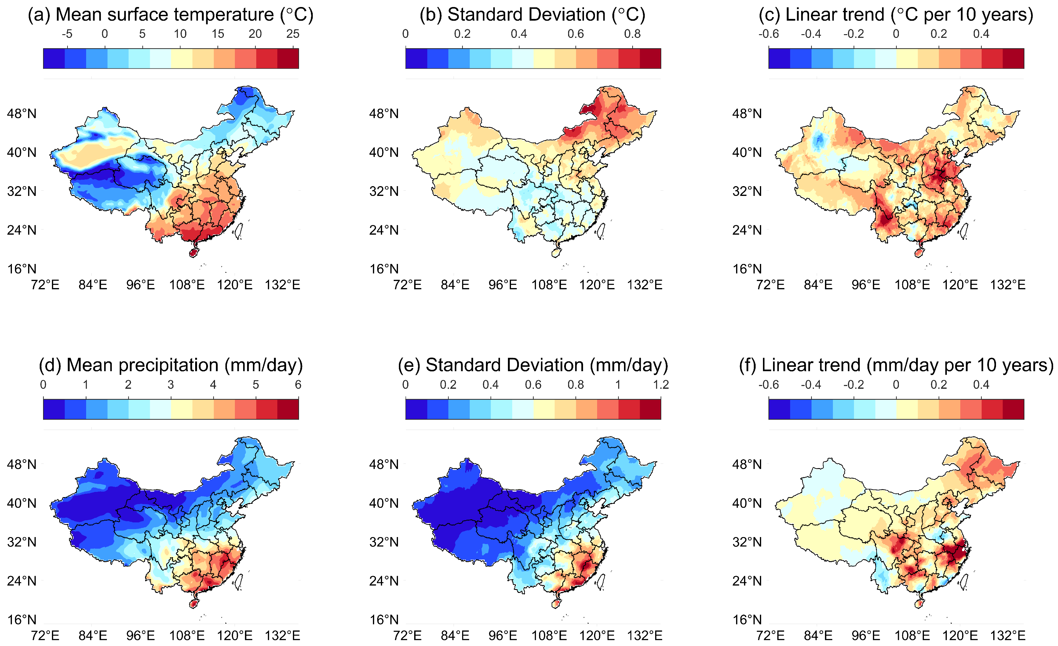
Figure 2.
Variations of national mean Food Security Index (FSI) and the sub-system indicators during 2002-2021.
Figure 2.
Variations of national mean Food Security Index (FSI) and the sub-system indicators during 2002-2021.
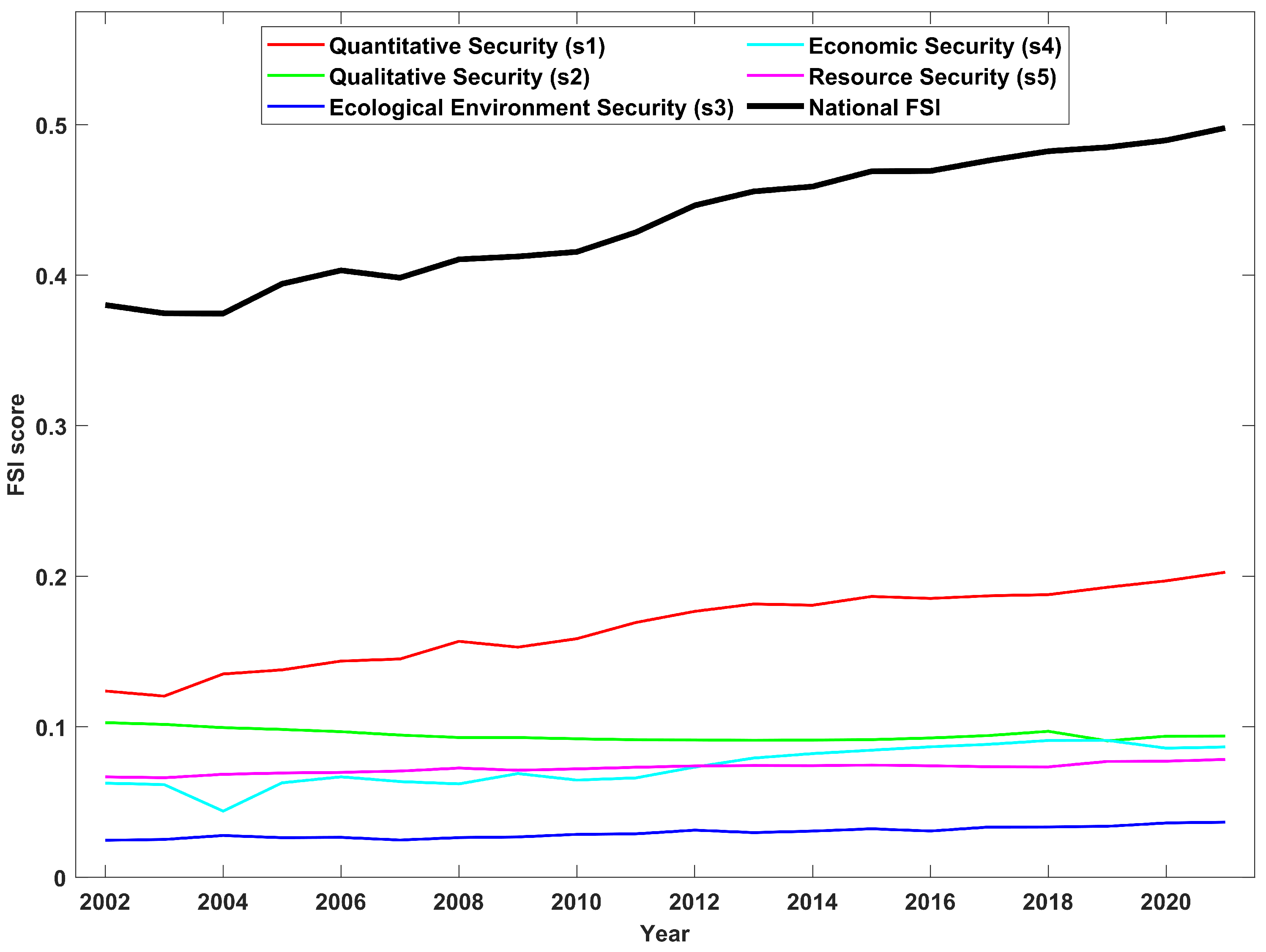
Figure 3.
Boxplot of the provincial on Dimensions of (a) space and (b) time.
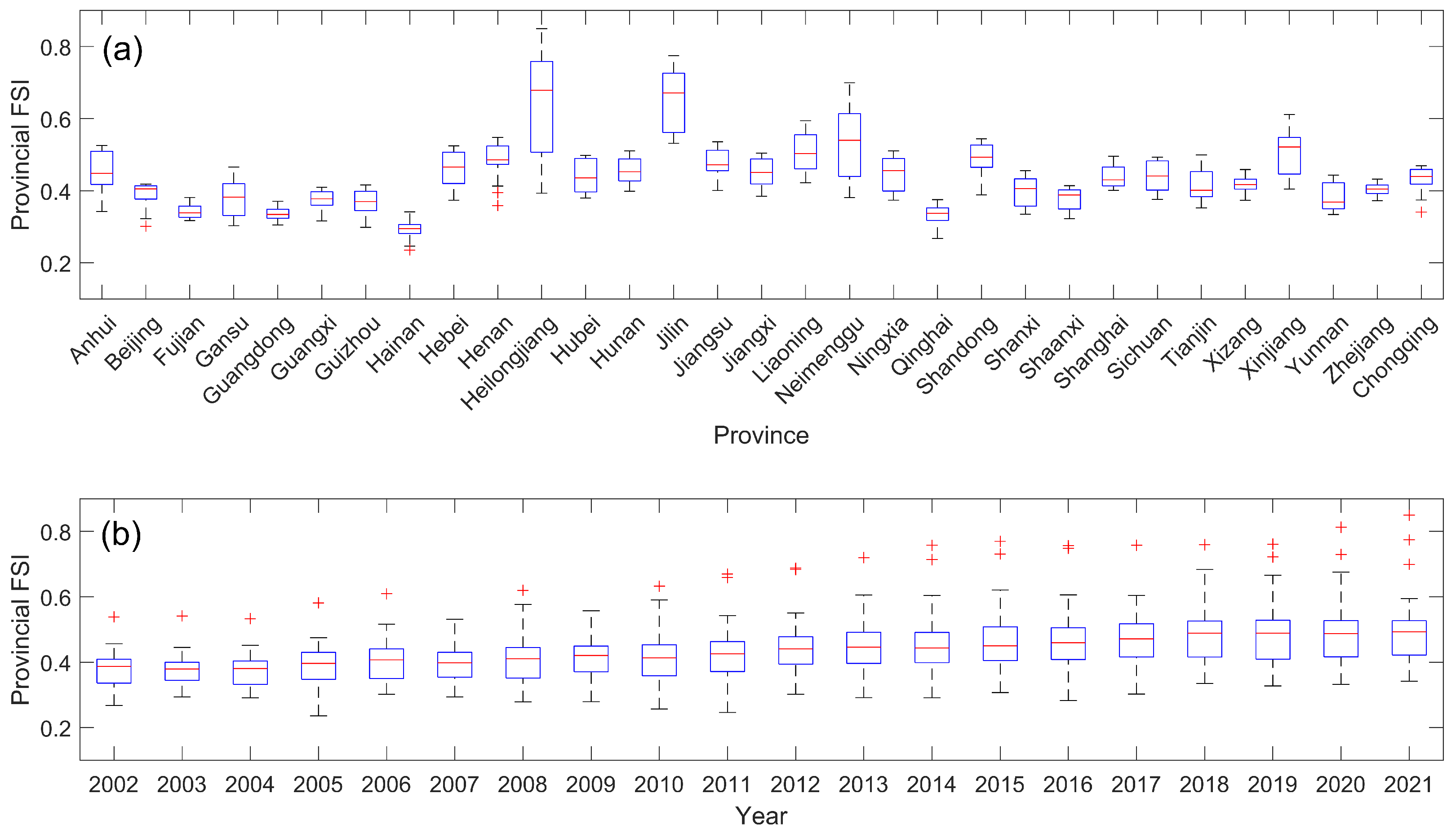
Figure 4.
Taylor diagram for evaluating the diversity of provincial . The angular distance from the x-axis denotes the temporal correlation coefficient between each provincial to national wide mean .
Figure 4.
Taylor diagram for evaluating the diversity of provincial . The angular distance from the x-axis denotes the temporal correlation coefficient between each provincial to national wide mean .
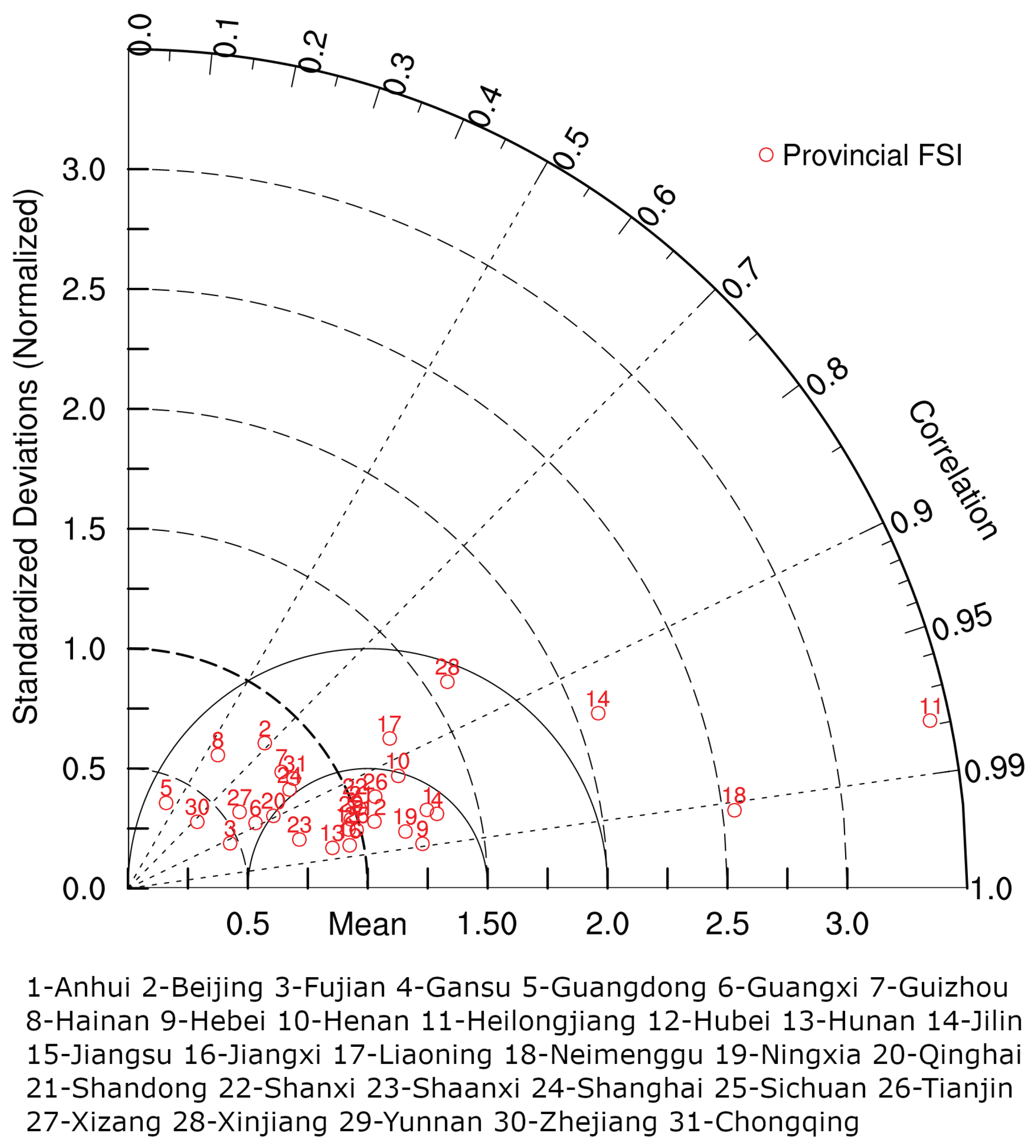
Table 2.
Weights of indicators in Food Security Indicator System involved in this study.
| Tier 2 Indicator | Tier 3 Indicator | Weight |
|---|---|---|
| s1 | j1 | 2.54% |
| j2 | 19.15% | |
| j3 | 41.25% | |
| s2 | j4 | 5.64% |
| j5 | 7.51% | |
| s3 | j6 | 3.78% |
| s4 | j7 | 3.08% |
| j8 | 7.67% | |
| s5 | j9 | 6.09% |
| j10 | 3.30% |
Table 3.
The linear impact of annual mean climate variables on China’s provincial Food Security Index (FSI) and its five Tier-2 sub-indicators, as enumerated in Table 1.
Table 3.
The linear impact of annual mean climate variables on China’s provincial Food Security Index (FSI) and its five Tier-2 sub-indicators, as enumerated in Table 1.
| Variables | s1 | s2 | s3 | s4 | s5 | FSI |
|---|---|---|---|---|---|---|
| -0.553*** | 0.137 | -0.272 | 0.418*** | -0.175* | -0.188*** | |
| (0.12) | (0.10) | (0.18) | (0.08) | (0.09) | (0.06) | |
| 0.063* | 0.024 | 0.061 | -0.022 | 0.010 | 0.024 | |
| (0.04) | (0.03) | (0.06) | (0.03) | (0.03) | (0.02) | |
| 0.242*** | 0.478*** | 0.114 | 0.002 | -0.066* | 0.176*** | |
| (0.05) | (0.04) | (0.07) | (0.03) | (0.04) | (0.02) | |
| 0.261*** | -0.267*** | -0.020 | -0.016 | 0.187*** | 0.087*** | |
| (0.05) | (0.04) | (0.08) | (0.04) | (0.04) | (0.02) | |
| -0.134*** | -0.079*** | -0.004 | 0.206*** | -0.001 | -0.026* | |
| (0.03) | (0.03) | (0.05) | (0.02) | (0.02) | (0.01) | |
| Constant | -0.811 | -4.957*** | -2.620 | -7.471*** | -2.159*** | -1.399*** |
| (1.08) | (0.88) | (1.68) | (0.78) | (0.83) | (0.50) | |
| Entity FE | Yes | Yes | Yes | Yes | Yes | Yes |
| Time FE | Yes | Yes | Yes | Yes | Yes | Yes |
| 0.652 | 0.381 | 0.366 | 0.859 | 0.298 | 0.758 | |
| Observation | 620 | 620 | 620 | 620 | 620 | 620 |
Standard errors in parentheses; *** p<0.01, ** p<0.05, * p<0.1; All variables being taken the logarithm.
Table 4.
Same as Table 3, but with the quadratic terms for and being incorporated.
Table 4.
Same as Table 3, but with the quadratic terms for and being incorporated.
| Variables | s1 | s2 | s3 | s4 | s5 | FSI |
|---|---|---|---|---|---|---|
| -0.512*** | 0.138 | -0.201 | 0.414*** | -0.152* | -0.166*** | |
| (0.11) | (0.10) | (0.18) | (0.09) | (0.09) | (0.05) | |
| 2.397*** | 0.088 | 4.076*** | -0.224 | 1.342*** | 1.321*** | |
| (0.41) | (0.34) | (0.63) | (0.30) | (0.32) | (0.19) | |
| -0.173*** | -0.005 | -0.297*** | 0.015 | -0.099*** | -0.096*** | |
| (0.03) | (0.03) | (0.05) | (0.02) | (0.02) | (0.01) | |
| 0.208*** | 0.478*** | 0.056 | 0.005 | -0.085** | 0.157*** | |
| (0.05) | (0.04) | (0.07) | (0.03) | (0.04) | (0.02) | |
| 0.253*** | -0.267*** | -0.035 | -0.016 | 0.182*** | 0.082*** | |
| (0.05) | (0.04) | (0.08) | (0.04) | (0.04) | (0.02) | |
| -0.116*** | -0.078*** | 0.027 | 0.204*** | 0.009 | -0.016 | |
| (0.03) | (0.03) | (0.05) | (0.02) | (0.02) | (0.01) | |
| Constant | -8.755*** | -5.174*** | -16.288*** | -6.781*** | -6.693*** | -5.814*** |
| (1.74) | (1.45) | (2.69) | (1.28) | (1.36) | (0.80) | |
| Entity FE | Yes | Yes | Yes | Yes | Yes | Yes |
| Time FE | Yes | Yes | Yes | Yes | Yes | Yes |
| 0.671 | 0.381 | 0.408 | 0.859 | 0.319 | 0.777 | |
| Observation | 620 | 620 | 620 | 620 | 620 | 620 |
Standard errors in parentheses; *** p<0.01, ** p<0.05, * p<0.1; All variables being taken the logarithm.
Table 5.
Same as Table 3, but for impact of climate extremes change.
Table 5.
Same as Table 3, but for impact of climate extremes change.
| Variables | s1 | s2 | s3 | s4 | s5 | FSI |
|---|---|---|---|---|---|---|
| -0.069*** | -0.028 | -0.155*** | 0.020 | -0.054*** | -0.041*** | |
| (0.03) | (0.02) | (0.04) | (0.02) | (0.02) | (0.01) | |
| 0.017 | 0.002 | -0.068* | -0.024 | -0.015 | -0.005 | |
| (0.03) | (0.02) | (0.04) | (0.02) | (0.02) | (0.01) | |
| 0.221*** | 0.484*** | 0.102 | 0.017 | -0.072** | 0.169*** | |
| (0.05) | (0.04) | (0.07) | (0.03) | (0.04) | (0.02) | |
| 0.250*** | -0.265*** | -0.020 | -0.007 | 0.183*** | 0.083*** | |
| (0.05) | (0.04) | (0.08) | (0.04) | (0.04) | (0.02) | |
| -0.137*** | -0.079*** | -0.015 | 0.205*** | -0.004 | -0.028* | |
| (0.03) | (0.03) | (0.05) | (0.02) | (0.02) | (0.01) | |
| Constant | -4.674*** | -3.660*** | -3.566*** | -4.231*** | -3.246*** | -2.595*** |
| (0.42) | (0.34) | (0.64) | (0.30) | (0.32) | (0.19) | |
| Entity FE | Yes | Yes | Yes | Yes | Yes | Yes |
| Time FE | Yes | Yes | Yes | Yes | Yes | Yes |
| 0.642 | 0.381 | 0.379 | 0.853 | 0.304 | 0.758 | |
| Observation | 620 | 620 | 620 | 620 | 620 | 620 |
Standard errors in parentheses; *** p<0.01, ** p<0.05, * p<0.1; All variables being taken the logarithm.
Table 6.
Same as Table 5, but with the quadratic terms for explanatory variables being incorporated.
Table 6.
Same as Table 5, but with the quadratic terms for explanatory variables being incorporated.
| Variables | s1 | s2 | s3 | s4 | s5 | FSI |
|---|---|---|---|---|---|---|
| 0.482** | 0.022 | -0.140 | -0.421** | 0.016 | 0.045 | |
| (0.23) | (0.19) | (0.35) | (0.17) | (0.18) | (0.11) | |
| -0.126** | -0.011 | -0.005 | 0.101*** | -0.016 | -0.020 | |
| (0.05) | (0.04) | (0.08) | (0.04) | (0.04) | (0.02) | |
| 1.054*** | 0.062 | 2.319*** | -0.160 | 0.730*** | 0.631*** | |
| (0.23) | (0.19) | (0.35) | (0.17) | (0.18) | (0.11) | |
| -0.086*** | -0.005 | -0.197*** | 0.012 | -0.062*** | -0.053*** | |
| (0.02) | (0.02) | (0.03) | (0.01) | (0.01) | (0.01) | |
| 0.197*** | 0.482*** | 0.073 | 0.028 | -0.083** | 0.160*** | |
| (0.05) | (0.04) | (0.07) | (0.03) | (0.04) | (0.02) | |
| 0.247*** | -0.265*** | -0.042 | -0.012 | 0.177*** | 0.078*** | |
| (0.05) | (0.04) | (0.08) | (0.04) | (0.04) | (0.02) | |
| -0.137*** | -0.080*** | -0.003 | 0.209*** | -0.000 | -0.026* | |
| (0.03) | (0.03) | (0.05) | (0.02) | (0.02) | (0.01) | |
| Constant | -8.135*** | -3.877*** | -10.416*** | -3.448*** | -5.442*** | -4.493*** |
| (0.80) | (0.66) | (1.20) | (0.59) | (0.61) | (0.37) | |
| Entity FE | Yes | Yes | Yes | Yes | Yes | Yes |
| Time FE | Yes | Yes | Yes | Yes | Yes | Yes |
| 0.658 | 0.382 | 0.428 | 0.855 | 0.325 | 0.773 | |
| Observation | 620 | 620 | 620 | 620 | 620 | 620 |
Standard errors in parentheses; *** p<0.01, ** p<0.05, * p<0.1; All variables being taken the logarithm.
Table 7.
Regional disparities in the influence of climate mean state changes on China’s provincial Food Security Index () by considering the distinct roles and characteristics of provinces within the context of food production and sales distribution.
Table 7.
Regional disparities in the influence of climate mean state changes on China’s provincial Food Security Index () by considering the distinct roles and characteristics of provinces within the context of food production and sales distribution.
| Variables | in MPA | in BA | in MCA |
|---|---|---|---|
| -0.155 | -0.114** | 0.024 | |
| (0.13) | (0.06) | (0.23) | |
| 0.042* | 0.111*** | -0.024 | |
| (0.02) | (0.03) | (0.03) | |
| 0.169*** | 0.125*** | 0.121** | |
| (0.03) | (0.04) | (0.05) | |
| 0.285*** | 0.004 | 0.010 | |
| (0.03) | (0.04) | (0.06) | |
| -0.029 | -0.063*** | -0.071* | |
| (0.02) | (0.02) | (0.04) | |
| Constant | -3.348*** | -1.443** | -1.503 |
| (1.17) | (0.57) | (2.06) | |
| Entity FE | Yes | Yes | Yes |
| Time FE | Yes | Yes | Yes |
| 0.889 | 0.811 | 0.615 | |
| Observations | 260 | 220 | 140 |
Standard errors in parentheses; *** p<0.01, ** p<0.05, * p<0.1; All variables being taken the logarithm.
Table 8.
Same as Table 7, but with the quadratic terms for explanatory variables being incorporated.
Table 8.
Same as Table 7, but with the quadratic terms for explanatory variables being incorporated.
| Variables | in MPA | in BA | in MCA |
|---|---|---|---|
| 3.321 | -1.233 | 5.616 | |
| (2.50) | (0.95) | (6.56) | |
| ( | -0.208 | 0.078 | -0.330 |
| (0.15) | (0.07) | (0.38) | |
| 1.866*** | 0.242 | 1.424*** | |
| (0.30) | (0.29) | (0.48) | |
| ( | -0.135*** | -0.010 | -0.104*** |
| (0.02) | (0.02) | (0.03) | |
| 0.123*** | 0.128*** | 0.129** | |
| (0.03) | (0.04) | (0.05) | |
| 0.283*** | -0.000 | -0.004 | |
| (0.03) | (0.04) | (0.06) | |
| -0.025 | -0.059*** | -0.038 | |
| (0.02) | (0.02) | (0.04) | |
| Constant | -23.615** | 2.056 | -30.319 |
| (10.31) | (3.48) | (28.54) | |
| Entity FE | Yes | Yes | Yes |
| Time FE | Yes | Yes | Yes |
| Observations | 260 | 220 | 140 |
| 0.905 | 0.813 | 0.646 |
Standard errors in parentheses; *** p<0.01, ** p<0.05, * p<0.1; All variables being taken the logarithm.
Table 9.
Same as Table 7, but for impact of climate extremes change.
Table 9.
Same as Table 7, but for impact of climate extremes change.
| Variables | in MPA | in BA | in MCA |
|---|---|---|---|
| -0.017 | -0.062*** | -0.019 | |
| (0.02) | (0.02) | (0.02) | |
| 0.019 | 0.028 | -0.031 | |
| (0.02) | (0.02) | (0.02) | |
| 0.172*** | 0.096** | 0.123** | |
| (0.03) | (0.04) | (0.05) | |
| 0.281*** | -0.003 | 0.012 | |
| (0.03) | (0.04) | (0.06) | |
| -0.027 | -0.073*** | -0.073* | |
| (0.02) | (0.02) | (0.04) | |
| Constant | -4.447*** | -1.334*** | -1.251*** |
| (0.33) | (0.37) | (0.36) | |
| Entity FE | Yes | Yes | Yes |
| Time FE | Yes | Yes | Yes |
| 0.888 | 0.815 | 0.620 | |
| Observations | 260 | 220 | 140 |
Standard errors in parentheses; *** p<0.01, ** p<0.05, * p<0.1; All variables being taken the logarithm.
Table 10.
Same as Table 9, but with the quadratic terms for explanatory variables being incorporated.
Table 10.
Same as Table 9, but with the quadratic terms for explanatory variables being incorporated.
| Variables | in MPA | in BA | in MCA |
|---|---|---|---|
| -0.002 | -0.066*** | -0.029 | |
| (0.02) | (0.02) | (0.02) | |
| 1.359*** | 0.233* | 0.981*** | |
| (0.21) | (0.14) | (0.30) | |
| ( | -0.108*** | -0.018 | -0.080*** |
| (0.02) | (0.01) | (0.02) | |
| 0.118*** | 0.097** | 0.135*** | |
| (0.03) | (0.04) | (0.05) | |
| 0.274*** | -0.009 | 0.022 | |
| (0.03) | (0.04) | (0.06) | |
| -0.024 | -0.072*** | -0.067* | |
| (0.02) | (0.02) | (0.04) | |
| Constant | -8.098*** | -1.860*** | -4.571*** |
| (0.65) | (0.51) | (1.06) | |
| Entity FE | Yes | Yes | Yes |
| Time FE | Yes | Yes | Yes |
| Observations | 260 | 220 | 140 |
| R | 0.905 | 0.817 | 0.655 |
Standard errors in parentheses; *** p<0.01, ** p<0.05, * p<0.1; All variables being taken the logarithm.
Disclaimer/Publisher’s Note: The statements, opinions and data contained in all publications are solely those of the individual author(s) and contributor(s) and not of MDPI and/or the editor(s). MDPI and/or the editor(s) disclaim responsibility for any injury to people or property resulting from any ideas, methods, instructions or products referred to in the content. |
© 2024 by the authors. Licensee MDPI, Basel, Switzerland. This article is an open access article distributed under the terms and conditions of the Creative Commons Attribution (CC BY) license (http://creativecommons.org/licenses/by/4.0/).
Copyright: This open access article is published under a Creative Commons CC BY 4.0 license, which permit the free download, distribution, and reuse, provided that the author and preprint are cited in any reuse.


