
Submitted:
06 March 2024
Posted:
08 March 2024
You are already at the latest version
Abstract
Software project estimating (SPE) is a powerful but necessary step in the production of projects for software. Software project estimating includes several components, estimating software time, software resources, software costs, and software effort estimation (SEE). SEE seeks to estimate the number of "hours-person" and "months-person" of work required for developing or managing a software program. During the initial phase of the development of software, future efforts are impossible to predict. To estimate effort, many deep learning (DL) and machine learning (ML) models were previously created. For estimate, single-model techniques and ensemble methods were investigated in this research. Ensemble methods involve a combination of multiple separate models. Bagging, boosting, and voting were the ensemble methods looked into for estimation. Datasets considered for estimation were COCOMO81, COCOMONasa I, COCOMONasa II, Albrecht, Maxwell, China, Desharnais, Desharnais_1_1, Kitchenham, Boehm, and Belady. The evaluation criteria used MAE, RAE, RMSE, RRSE, and CC. The result from previous studies is that the total size of the set of data utilized is small in predicting the effort, as the largest size of the set of data used is the China dataset containing only 499 projects. So, in this study, the dataset has been merged to increase the total size of the set of data and increase the accuracy of prediction. The results indicated that the suggested merged dataset increased effort estimation accuracy.
Keywords:
Artificial Intelligence(AI)
; Bagging
; Boosting
; ComImp
; Effort Estimation(EE)
; Ensemble Learning(EL)
; Machine Learning(ML)
; Merge Dataset
; PCA-ComImp
; Voting
; Random Forest(RF)
; Software Project Management(SPM)
; Software Effort Estimation(SEE)
1. Introduction
The accurate Effort Estimation (EE) is also a member of the most essential assignments in Software Project Management(SPM). Since it has a significant impact role in the achievement of software projects, among other factors. A low estimate leads to schedule/budget delay and performance agreement, whereas an overestimation wastes resources[29]. A rising amount of research is being conducted to increase the estimation accuracy of the development of software. efforts by applying algorithms. of Artificial Intelligence(AI) in recent years. Nevertheless, All the available models are appropriate for every situation. This model’s performance is unreliable because it fluctuates from dataset to dataset.
COCOMO it is known as the "Constrictive Cost Model" and is mostly used for SEE. It forecasts the total cost of the design, the listed time for the design, and the amount of trouble required for the design. Additionally, it calculates how many Man-Months (MM) are required to complete the development of software applications[23].
The COCOMO model provides a lot of benefits, but it also has significant drawbacks. One of these is that the estimation changes with time [23]. The COCOMO model also relies on previous project data, which isn’t always easily accessible [24]. The COCOMO prototype is unable to estimate every phase of the "Software Development Life Cycle (SDLC)" [24]. Regarding the COCOMO model to work, A huge quantity of data is required. As a result, the industry will have to invest a lot of time in project estimation. However, there are significant issues with this approach, including the number of projects that should be evaluated and the limitation of the project’s attributes to data accessible at the start of the evaluation procedure [24].
Machine Learning (ML) approaches have lately become crucial in the field of software studies. Most likely in many other domains of science, ML methods are being employed and put into practice [3]. The quick evolution of the software cost estimation process and planning time, which could include technological advancements, team expertise, tools, and programming languages available, makes ML techniques superior to certain other approaches that may just focus on work in statistics and mathematics [3]. ML may be a good approach to create the suggested model because it can study from prior data and adjust to the broad range of deviations that come with a software project’s progress.
The prior study[28], employed a small sample size of a dataset containing only 499 projects and compared across various models, including Ada-boost regression, K-nearest neighbor(KNN), Decision Trees(DT), bagging regressors, Random Forest Regressors(RFR), gradient boosting(G-Boosting). According to the results, which show an accuracy of 93%, the G-boosting regressor model is outperforming with greater accuracy.
The objective of the current research is to expand the size of a dataset by using 1200 software projects collected from many open sources. The dataset definition is in Table 1. Moreover, a suitable approach must be identified and defined to provide an estimate that is as near to the actual effort as possible. The EL techniques/prediction models (Bagging, Boosting, and Voting) are utilized and implemented to the dataset, and its results are contrasted with different models to get more accuracy.EL is a method that combines multiple learning algorithms to produce more accurate predictions than could be obtained from any of the constitutive learning algorithms singly. In contrast to a statistics ensemble in statistics mechanics, which is typically infinite, an ML ensemble only comprises a finite collection of potential models, but usually provides for an even more adaptable model to there are some of those options to produce a better precision for EE. The results were evaluated and compared using different metrics MAE, RAE, RMSE, RRSE, CC.
2. Research Question
The primary objective of the present research is to analyze the three research questions that follow: RQ1: How can EL be applied to SEE? What is the best EL(Bagging, Boosting, Voting) approach, and what are the benefits of using this approach? RQ2: How can we evaluate the performance of an EL-based method for SEE, and what are the appropriate metrics to use? RQ3: Merging different projects from several open sources can potentially improve the performance of an EL model, instead of using a small size of projects.
3. Literature Review
Three main techniques can be used to categorize software effort assessment methods: expert opinion, algorithmic models, and Artificial Intelligence(AI) [31,32]. Estimates made by specialists are based on their prior work on related projects. The level to which a new project aligns with the expert’s expertise and skill sets determines how accurate this strategy is. A recent experiment revealed that expert judgment-based estimates of software development efforts display a considerable degree of variation [30]. As a result, the estimation procedure is not explicit and cannot be repeated [31].
The relationship between a software project’s characteristics, typically its size, and its development effort is represented by algorithmic models. These models are parametric, parameterizing from historical data using a standard form formula. COCOMO [34], and function points analysis [33] are a few examples of these models. The algorithmic models of relationships are too complex for algorithmic models to fully understand.
Recently, there has been a widespread use of AI techniques for SEE. Regression Trees(RT), and Naive Bayes Classifier (NBC) [35], Fuzzy Logic(FL) [36], Neural Networks(NN) [32,37], Bayesian Networks(BN)[38], Case-Based Reasoning(CBR) [39], Support Vector Regression(SVM) [2,41], and Genetic Programming(GP), Manual StepWise Regression(MSWR) [14,40] are a few examples. AI models have several benefits, such as their capacity to represent the intricate interrelationships between effort and their capacity to acquire knowledge from past project information [42].
There aren’t many homogeneous EL models that have been created and assessed specifically for SEE. The application of bagging predictors in SEE was examined in [34]. An ensemble of NN with Associated memory was studied to estimate software development expenses. By averaging across a heterogeneous ensemble of numerous learners in assessed the group. Nevertheless, there was no improvement in the software work estimation accuracy[43].
SEE is a critical task in SPM. ML has been widely used to develop models for SEE. In this literature review, we summarize some of the recent studies that have used ML and EL for SEE.
3.1. ML Methods for SEE Review
Software effort is typically estimated using a variety of methods that have been published by scholars all over the prior years. The function based on the points model, the COCOMO model, and the computation of effort utilizing previously collected information in a unique formula were the initial three techniques for EE of commonly used software. Software development EE has been made with great success using ML methods. By using these ML algorithms, specialists can focus more of their time on other software system tasks that meet client needs and less time on assessing the proposed project. Several researchers have utilized ML to measure effort over the last ten decades.
The validation method was used in [26]. They compared the Random Forest(RF) model they had developed to the Regression Tree(RT) model depending on three separate datasets: Tukutuku, ISBSG, and COCOMO. The instruments employed for evaluation include Sum Squared Error(SSE), Mean Magnitude of Relative Error(MMRE), Relative Standard Deviation(RSD), Standard Accuracy(SA), Evaluation Function (EF), Median Magnitude of Relative Error(MdMRE), and Prediction(Pred). Depending on the findings, the performance of the RF design is superior. [26].
This Paper [35] offered a model SVR for SEE that utilized several project-related features such as code size, requirements volatility, and development experience. The authors evaluated the model on three datasets. According to the findings, the SVR-based model performed better than traditional statistical models and achieved advanced outcomes. In [13] offered a model of Artificial Neural Networks (ANN) for SEE that used features like these "function points(FP)", "lines of code(LoC)", and development skills. The authors evaluated the model on six datasets. Depending on the findings, the ANN framework operated better than traditional statistical models and achieved advanced outcomes. Also, Paper [6] offered a model RF for SEE that utilized several project-related features such as code complexity, development experience, and team size. The authors evaluated the model on six datasets. According to the findings, the RF-based model performed best than traditional statistical models and achieved advanced outcomes.
Also in [44], Finding the best accurate ML algorithm is the primary objective of the computation of three different algorithms. They utilized SVM, Multi-layer Perceptions(MLP), and Linear Regression (LR) techniques on the "Software Engineering in the Republic of Sudan(SEERA)" dataset to forecast the quantity of effort and time required to finish the project. To analyze the predictive model’s accuracy in forecasting the resources and time needed. to build software, they have examined the Mean Squared Error(MSE), MAE, and Root-Squared(R-squared) assessment metrics. Consequently, the R-squared for LR is 0.95, the SVR is less than 0.04, and the MLP score is 0.83. The LR model outperforms the MLP and SVR algorithms as well as the accuracy of predictions, according to the results.[44].
3.2. EL Methods for SEE Review
SEE is a major role in software engineering, and EL became known as a potential method to develop models for this purpose. This literature review discusses some recent studies that have used EL for SEE.
There has been much research done on ensemble SEE so far. Several single estimating procedures were ensembled, resulting in unique estimations with comparable high accuracy. Using voting ensemble models, the five different models MLP, RT, Radial basis function(RBF), SVM, and KNN have been compared [21]. The results indicated that the models are inaccurate and perform differentially among diverse datasets. The combined model outperforms all other models with an MMRE of 0.61 and a PRED of 37.50%. They created three EL models in this study [19] by utilizing KNN, RT, MLP, and SVM techniques. The models were tested using datasets from Albrecht and Miyazaki. The findings show that there is no optimal absolute EL model compared to the individual approaches because the suggested ensemble’s performance differs depending on the dataset.
Additionally, the combination of MLP Neural Network(MLPNN) on Ridge, Lasso, Bagging, and AdaBoosting has been researched [20]. The outcomes showed that AdaBoosting-MLPNN increased the accuracy to 82.2% compared to using MLPNN only resulted in an accuracy of 78%. The ensemble averaging of three ML algorithms, SVM, and KNN, was proposed in [18]. The EL models were more accurate than the single model, the EL model increased accuracy from 85% to 91%.
These studies used a small sample size of datasets across different models, according to previous research results, showing a high accuracy of 93% on a dataset size of 499 projects.
ML techniques, such as classification approaches, clustering methods, regression techniques, NN, and EL methods, are frequently used to SEE. The survey of SEE utilizing different methods, estimation datasets, assessment metrics, results, and discussion from each work are all detailed in Table 10.
4. Back Ground
4.1. Machine Learning (ML)
ML is a category of AI. AI in computers is produced using a variety of learning strategies. Consequently, there are many different kinds of ML, such as supervised learning, deep learning, evolutionary learning, and reinforcement learning [46]. To create models depending on the dataset’s learning, ML algorithms like KNN, RF, RT, LR, NN, NB, SVM, etc. are utilized. The dataset will be utilized for testing and training to generate the ML models. The importance of ML is that it continually keeps up with the environment, and the model continually enhances itself by learning from data or knowledge. Using ML, you can reduce mistakes made by humans and effort. [46].
ML has been used to predict effort and cost for software projects. One can measure the accuracy of ML algorithms used for estimation by computing metrics such as MMRE, RMSE, RSE, MdMRE, SSE, RSD, SA, EF, etc [46].
Two categories apply to ML algorithms:
- Supervised Learning: There are examples in every dataset used in ML. Features are used to define or represent the instances. These characteristics may be "continuous" or "binary/categorical". Marked instances are those that match the correct output or response. After the dataset (training and testing data) is marked, supervised machine learning techniques are utilized. Using marked previous and present data, these systems analyze and forecast. [47]. Classification and Regression types of supervised learning. A collection of classes exists in the output space of a supervised learning problem called classification [47]. One kind of supervised learning issue is regression, in which a set of continuous values serves as the output space. By statistical approaches, methods of regression, estimate the relationship between the output and factors that affect the result[47].
- Unsupervised Learning: is used in place of supervised learning for cases that are not marked. To create a function that explains the data’s pattern, the unsupervised algorithms examine the information without marking[48]. These methods don’t provide very accurate output identification. Nonetheless, these techniques are useful for identifying and documenting findings about the data’s latent patterns. Unsupervised learning includes association and clustering[48].
4.2. Algorithms
The supervised ML algorithms and ensemble techniques used in this research to construct the EL model are listed below, following the completion of the basic literature review and the supervisor’s recommendations. The chosen supervised ML algorithms used in this research are briefly explained below:
4.2.1. K-nearest neighbors (KNN)
The techniques based on supervised peers are applied to regression and classification issues alike. "Non-generalizing" ML techniques are those that use neighbors. Case-based reasoning, which includes actions like locating cases, locating related cases, and adopting cases, is the fundamental idea underlying these techniques[49]. Neighbors-based techniques are as straightforward and effective as they seem. When the labels on the data are continuous, regression neighbors-based techniques are applied. The average of "k" of the target label’s closest neighbor labels serves as the basis for The forecasting or evaluation of the target labels. The user provides the value (integer) of ’k’ [49].
The concept behind KNN’s operation, namely analogy reasoning, is straightforward to comprehend, and its non-generalizing and non-parametric methods are among its benefits[49].
One potential challenge when utilizing KNN is that the technique’s prediction rate relies on the data’s availability, and poor feature scaling may have an impact on how well it performs [49]. To address these constraints, we have standardized the data and carefully chosen the features.
4.2.2. Decision Tree (DT)
DT is a nonlinear approach that seeks to create a model using decision rules learned from data features. By using the rules as a guide, the model forecasts the target variable. When addressing regressor difficulties, the DT Regressor is employed. The following are some benefits of DTs: They are simple to comprehend and apply; They require little data preparation; and they can handle a variety of data kinds, including categorical and numerical data[15].
One potential challenge when utilizing DT is that it can be challenging to comprehend the idea of how DT operates. Since DTs are sensitive to even minute changes, using them with ensembles is advised. To address them, we conducted a thorough background investigation on the methodology and applied DT using an ensemble approach to get rid of the sensitivity with variation in our study[15].
4.2.3. Navies Bayes (NB)
A variant of the Bayesian network classifier, the NB classifier is constructed by the assumption that the variables, given the class variable, are conditionally independent. A NB structure does not allow for any more connections. Because of its benefits over other classifiers, NB has been utilized as an excellent classifier for a long time. It works incredibly well over a wide range of domains, is efficient, robust against noisy or missing data, and is comparatively easy to apply[50].
4.3. Ensemble Learning (EL)
Through the combination of forecasts from several learning algorithms/estimators, ensemble approaches attempt to increase an estimator’s robustness.[51]. Three types of ensemble methods can be defined:
- Methods for averaging: The goal is to create and forecast using a variety of estimators, and then average these forecasts. Because of a lower variance, it is claimed that the estimator combined by employing the average technique outperforms an individual estimator on average. Random forest trees, bagging, and other average ensemble techniques are a few examples[51].
- Methods for boosting: These techniques aim to create an effective ensemble by combining several weak estimators, as opposed to averaging ensemble methods. By developing single estimators one after the other, these techniques aim to reduce the ensemble’s bias. Boosting ensemble techniques include adaboost, gradient tree boosting, and others[51].
- Methods for voting: A voting classifier is an ML model that is trained on a wide EL of models and forecasts an output (class) depending on the models’ largest potential of providing the desired class.[51].
4.3.1. Bagging
Bagging creates an EL model by periodically creating occurrence groups (with substitution) from the source training datasets and then implementing a learning model to each of the occurrence subsets, such as a regression tree for general scenarios. The overall projected value is the mean of all the calculated estimates. Theoretically, the error caused by unfavorable model variance can be minimized by any ensemble technique based on independent sampling [49].
Furthermore, feature randomness and bagging are combined by the random forest algorithm to create an uncorrelated forest of decision trees, which is considered an enhancement above the bagging method.
4.3.2. Random Forest (RF)
RF is a meta-averaging algorithm. that builds several decision trees on various dataset subsets to increase prediction accuracy and reduce overfitting [6]. Each estimation’s values are averaged and provided as the final output. When there are continuous target values, the RF Regressor is used.
4.3.3. AdaBoosting
The fundamental idea underlying the well-known boosting approach AdaBoost is to combine weaker estimators and apply them to better data types. The outcomes for every forecast are then aggregated by balancing the vote of the majority or strict vote. The Adaboost regressor is a tool for addressing regression issues.[20].
5. Methodology
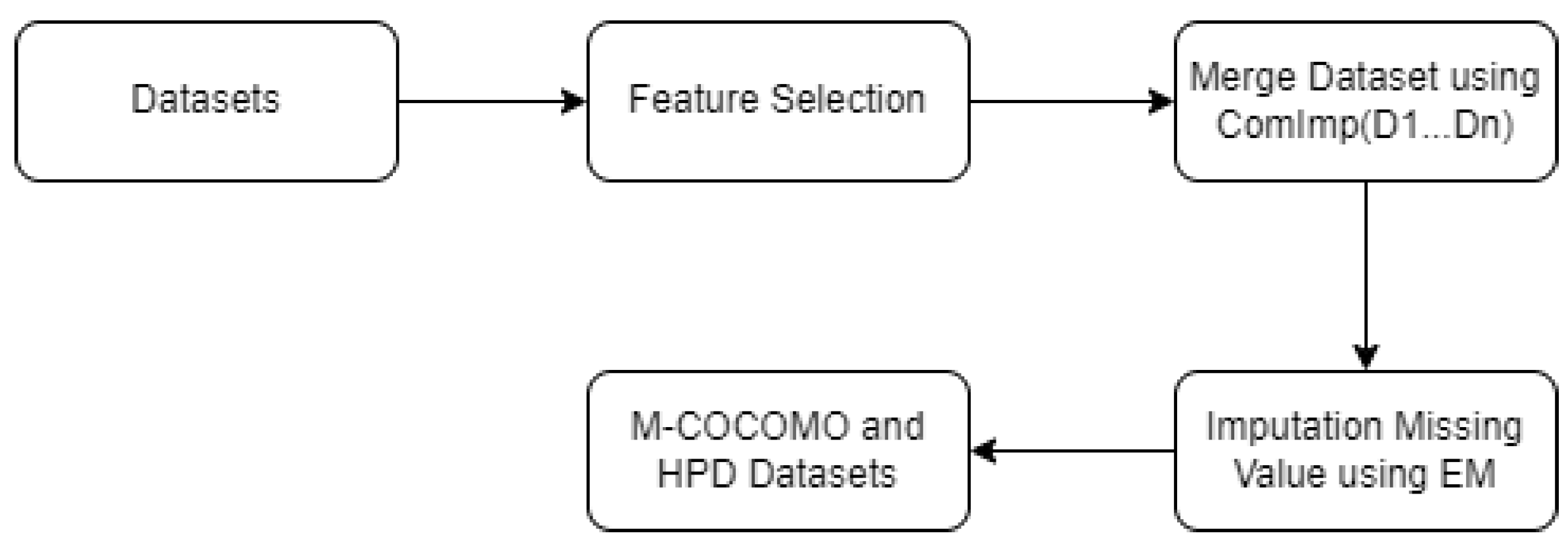
Based on the conclusions of the literature review and associated investigation, we have decided to use the EL (bagging, Boosting, and Voting) method to empirically create an efficient method for SEE in our research. The motivation is that few research have looked at this method, and its simple yet successful benefits encourage us to experiment with it. The result based on the findings obtained in the associated research shows that the size of the collection of the dataset utilized is small in predicting the effort, as the largest size of the collection of the dataset used is the China dataset containing only 499 projects. Therefore, the major purpose of this research is to expand the size of a dataset by using 1200 software projects collected from many open sources. The EL prediction models (Bagging, Boosting, and Voting) are utilized and implemented into the dataset, and their results are contrasted with different models to get more accuracy. The suggested methodology of SEE is illustrated in Figure 1, and each phase will be discussed thoroughly in the research sections.
6. Dataset
6.1. Dataset Collection
To investigate the resilience and flexibility of the constructed model, it can be helpful to select various datasets that vary in terms of size and feature count. The choice of datasets depends on the available research survey we completed to learn more about the datasets used to estimate software development efforts.
The selected datasets were gathered based on "Predictor Models in Software Engineering (PROMISE)" repository [58], and this makes datasets accessible to the public for use in Software Engineering-related studies and research. GitHub dataset search was also utilized by us.
6.2. Datasets Description
The selection of eleven datasets is freely accessible to the public and was heavily used in numerous earlier research to estimate software development efforts[1,2,3,4,5,6,7,8,9,10,11,12,13,14,15,16,17,18,19,21,22,23,24,25,25].Table 1 is a summary of each dataset’s description. The descriptions for each dataset utilized in this research are listed below. And explaining the Feature Selection(FS) from each dataset according to previous research[1,2,3,4,5].
6.2.1. COCOMO81
The COCOMO81 dataset [1] was frequently used to validate different methods of EE. There are 63 software projects in all, and each one is explained by 17 features and a concerted effort. In COCOMO81, the dataset calculates the actual effort in “person-months”, or the time required for a single person to complete a project. Table 2 gives a detailed explanation of the COCOMO81 repository.
6.2.2. COCOMONasa I
The COCOMONasa I dataset[2] was frequently used to validate different methods of EE. There are 60 software projects in all, and each one is explained by 17 features and a concerted effort. In COCOMONasa I, the dataset calculates the actual effort in “person-months”, or the duration of time required for a single person to complete a project. Table 3 gives a detailed explanation of the COCOMONasa I repository.
6.2.3. COCOMONasa II
The COCOMONasa II dataset[5] was frequently used to validate different methods of EE. There are 93 software projects in all, and each one is explained by 24 features and a concerted effort. The COCOMONasa II dataset computes the real effort to make sense of "person-months," or the duration of time needed for a single person to complete a project. A thorough description of the COCOMONasa II repository may be found in Table 4. The COCOMONasa II dataset includes 93 projects and twenty-four attributes. Of these, seven (record number, project name, forg, cat2, center, mode, and year) are not effort multiplier effects, therefore we can exclude them.
6.2.4. KITCHENHAM
6.2.5. DESHARNAIS
Eighty-one software projects from Canadian software companies made up the initial version of the Desharnais dataset [8]. Nine features make up this dataset. The dataset calculates the actual effort in"person-hours", or the duration of time required for a single person to complete a project. The Desharnais dataset is fully described in Table 6.
6.2.6. DESHARNAIS_1_1
Eighty-one software projects from Canadian software companies made up the initial version of the Desharnais_1_1 dataset[8]. Twelve features make up this dataset. The dataset calculates the actual effort in"person-hours", or the time required for a single person to complete a project. The Desharnais_1_1 dataset is fully described in Table 7.
6.2.7. MAXWELL
The 62 projects in the Maxwell dataset[20], it was assembled based on of Finland’s biggest commercial lending institutions, and are each characterized by 23 features. Table 8 offers an extensive overview of the Maxwell dataset. In Maxwell, the dataset calculates the actual effort in “person-hours”, or the duration of time required for a single person to complete a project.
6.2.8. BELADY
6.2.9. BOEHM
6.2.10. CHINA
There are 14 features in the China dataset[9] used to predict software effort. In total, there are 499 distinct project instances. The dataset calculates the actual effort in"person-hours", or the time required for a single person to complete a project. The China dataset is fully described in Table 11.
6.2.11. ALBRECHT
A publicly accessible dataset that contains information useful for estimating SDE is called Albrecht[4]. The dataset includes 24 projects, eight features all numeric values. This dataset’s objective feature is effort, which stands for real effort. The dataset calculates the actual effort in"person-hours", or the time required for a single person to complete a project. The Albrecht dataset is fully described in Table 12.
6.3. Merge Dataset
Merging data from several datasets can be useful in many use scenarios to enhance the accuracy of an ML model, particularly when there are few samples in a minimum of one of the various datasets[59].
When it comes to executing any type of ML technique, the dataset size is believed to be the most important component. When there’s not enough information for a model to develop, the forecasts that it makes may be unreliable[59]. The datasets used in the present research are freely accessible, and the number of data points associated with these databases is similarly limited. However, I need to merge datasets to increase the size of the data and enhance the accuracy of prediction.
In this research, the data set used in Table 1 has been divided into two parts according to the output feature effort, monthly or hourly that can be defined below:
- Merge COCOMO81, COCOMONasa I, and COCOMONasa II to produce a new Month-COCOMO(M-COCOMO) dataset containing 216 projects with 17 features.
- Merge China, Maxwell, Desharnais, Desharnais_1_1, Albrecht, Kitchenham, belady, and Boehm to produce a new hours phase dataset(HPD) dataset containing 988 projects with seven features.
Even though some features from these sets of datasets are shared by all of them, there is still a further difficulty in these situations because the features from each dataset differ. We utilized an entirely novel structure identified as Combine datasets based on Imputation (ComImp) to address this after making a feature selection[59]. Additionally, we utilized PCA-ComImp, a ComImp variation that applies Principle Component Analysis (PCA), in which dimension reduction is carried out just during dataset merging. This is helpful in cases where there are a lot of unique features in the datasets[59].
6.3.1. ComImp (Combine Datasets Based on Imputation)
A structure called ComImp enables the vertical combination of datasets through the imputation of missing data. When equivalent features in one dataset cannot be found in the dataset but can be found in another component dataset, the algorithm inserts columns of missing entries into the datasets that are intended to be merged, therefore vertically stacking the datasets by overlapping features (weight). Using the stacking data to impute missing values[59]. In this research, the Expectation-Maximization(EM) technique is utilized to impute missing data[57]. The proposed ComImp for the merged dataset is shown in Figure 2
Below is the summary of each dataset produced after making ComImp:
- M-COCOMO: The M-COCOMO dataset was frequently used to validate different methods of EE. There are 216 software projects in all, and each one is explained by five features and a concerted effort. In M-COCOMO, the dataset calculates the actual effort in "person-months", the time required for a single person to complete a project. . The result is no missing value after merging these datasets. Table 13 provides a full explanation of the M-COCOMO repository.
- HPD: There are twelve features in the HPD dataset used to predict software effort. In total, there are 988 software projects in all. The dataset calculates the actual efforts in"person-hours", the time required for a single person to complete a project. The result missing value after merging these datasets. The HPD dataset is fully described in Table 14.
Figure 2.
ComImp for merge datasets
6.3.2. ComImp that utilizes Principle Component Analysis (PCA-ComImp)
Sequential operations can merge various datasets with several attributes that are not common. For instance, let’s say we have ,.. . Next, we may merge and to obtain , and then and to obtain , and so on.
- Attributes analysis: The set of features (data columns) for each data source is recognized and identified. This helps to recognize how various attributes reflect various information and which must be included for the vertical scale of your combined data to change.
- Fined the intersection between and , to produced .
- Then fined , It indicates that is the collection of features that are part of but not . is equivalent.
- Redused dimension of the dataset using PCA: ,.
- Finally, produced .
- Next, similar to ComImp, we produced HPD, stacked them together, and imputed them.
- For missing values, in this research, the EM technique was used to impute missing data.
Below is the summary of each dataset produced after making PCA-ComImp:
- M-COCOMO: The M-COCOMO dataset was frequently used to validate different methods of EE. There are 216 software projects in all, and each one is explained by 17 features and a concerted effort. In M-COCOMO, the dataset calculates the actual effort in "person-months", the time required for a single person to complete a project. The result is no missing value after merging these datasets. Table 15 gives a detailed explanation of the M-COCOMO repository.
- HPD: There are seven features in the HPD dataset used to predict software effort. In total, there are 988 software projects. The dataset calculates the actual effort in "person-hours", the time required for a single person to complete a project. The result missing value after merging these datasets. The HPD dataset is fully described in Table 16.
7. Data Pre-Processing
7.1. Feature Selection (FS)
Eliminating unnecessary and redundant data is the primary function of FS, which helps to increase the estimation’s accuracy. Essentially, FS is carried out on sampling data sets to raise the estimations’ score for accuracy. One of the actions carried out during the reprocessing stage of an estimation is feature selection. FS has several key benefits, including removing unnecessary attributes, reducing data size, simplifying the data mining procedure, and identifying relevant features [52].
7.2. Standardization of Features(SF)
It is generally required to standardize features in advance of applying ML algorithms into practice. Effective feature standardization is done by eliminating mean values and scaling data depending on variance in units. [53]. The following procedure is used to calculate the standard scale for a sample "y" in Equation (1)
where could represent either zero or the mean of the training samples under evaluation [53]. The standard deviation of the training sample under evaluation is denoted by .
The dataset is standardized before being divided into training and testing once the dataset has been separated into two sections: "target," which stores the target elements, and "source," which stores the remaining elements. The data in Figure 5 and Figure 6 below shows the COCOMO81 dataset before and after standardization. Every dataset is standardized using the same process as the COCOMO81 dataset.
7.3. Imputation Missing Values
The imputer for ComImp should be selected based on several characteristics, including quick, imputation quantity, and sample-by-sample prediction ability, ignoring the fact that there are numerous imputation techniques available. For limited datasets, imputation quality can be achieved by slow approaches like kNN, MICE, and missForest [55], which can be taken into consideration. These techniques cannot be applied to high dimensional data, though, as they may be too slow for comparatively large-size data [55].
In this research, they used EM to impute missing values after the merge dataset, because the data type numerical other techniques need categorical data type, and do not use all the attributes for classification. In large sample sizes (more than 30), the EM technique outperformed the other methods; its effect size values matched more closely with the effect size values of the entire data set with all possible loss ratios[57].
EM a technique for determining the highest probability estimation of the model parameters is the EM technique. The maximum probability of estimations for the missing data is generated using the method of iteration. The ease of use and variety of cases that can be handled by this method are its defining features[56]. This approach leverages all available information from both complete and incomplete situations by imputing missing data using estimates derived from a repetitive estimating procedure. Based on preliminary estimates of the model’s parameter values, the missing data is predicted; these predictions are then used to adjust the parameter values, and the prediction process is repeated with the adjusted model parameters until the parameters are close to the highest probability estimates[56].
8. Performance Evaluation
The metrics listed below are utilized to evaluate the performance of the EL algorithms :
8.1. Mean Absolute Error (MAE)
8.2. Root Mean Squared Error (RMSE)
It computes the mean-variance among the actual values and the values predicted by a model. It provides a rough estimate of the accuracy, or how well the model can forecast the expected outcome [1]. As shown below, the RMSE for every observation ’i’ across ’n’ samples can be computed as follows in Equation (3).
8.3. Relative Absolute Error (RAE)
RAE determines a predictive model’s accuracy. ML can make use of RAE. Additionally, RAE can be represented as a percentage that calculates the average error or residual of errors generated by a simple[1]. If the result is less than 1, the model will be considered non-trivial. As shown below [1], the RAE for every observation ’i’ across ’n’ samples can be computed as follows in Equation (4).
8.4. Root Relative Squared Error (RRSE)
The RRSE is used for normalizing the average after the average errors are squared. To keep the errors within the exact same length, the square root is then calculated [1]. If the result is lower than one, the model will be considered non-trivial[1]. The following formula can be used to determine the RRSE for each unique observation "i" over "n" samples in Equation (5).
Where,
8.5. Correlation Coefficient (CC)
The mathematical connection between two variables is measured by the CC. The variables could be a dataset’s columns. A strong connection exists when the CC is larger; a weak connection occurs when it is lower[1].
9. Result & Discussion
Previously, an enormous amount of datasets were used to assess and apply models for SEE. The datasets used in the present research are freely accessible, and the number of data points associated with these databases is similarly limited. The datasets considered were COCOMO81, COCOMONasa I, COCOMONasa II, Albrecht, China, Desharnais, Desharnais_1_1, Maxwell, Kitchenham, Boehm, and Belady. However, I need to merge datasets to increase the size of the data and enhance the accuracy of prediction.
The new datasets are created from datasets in Table 1:
- M-COCOMO contains 216 projects from merging (COCOMO81, COCOMONasa I , and COCOMONasa II) by two methods of merging(ComImp and PCA-ComImp).
- HPD contains 988 projects from merging (Albrecht, China, Desharnais, Desharnais_1_1, Maxwell, Kitchenham, Boehm, and Belady) by two methods of merging(ComImp and PCA-ComImp).
Since the results of earlier studies were presented using various performance criteria, several metrics are taken into account while comparing and assessing the findings MAE, RAE, RMSE, RRSE, and Correlation Coefficient (CC). Low values for RMSE, MAE, RAE, and RRSE, and high values for CC characterize an appropriate estimate model.
Where MAE is an indication of the average absolute variance between the actual and forecast values, RMSE demonstrates that it is more vulnerable to bigger errors due to the squaring process, and RAE is a percentage of the average absolute error relative to the observed values’ mean. It gives a measure of error normalized by the data scale, while RRSE provides a relative measure of error compared to the average of the observed values. It is a normalized measure, similar to RAE, with CC signifying a very strong positive correlation between expected and actual values. A close to 1 number indicates a strong linear relationship, and accuracy is the percentage of accurately predicted instances compared to all instances.
Different EL techniques available were Bagging, Boosting, and Voting. For the EL(bagging and Boosting), these models need to put the value of the estimator,(where the estimator is the number of models combined) the result after experiencing the values from two models to ten models is the ten models is the best value of estimator. Bagging is combined by the RF and Boosting is Combined by the DT. The Voting model contains individuals ML (NB, KNN, and DT).
The results of the EL model generated (Bagging, AdaBoosting, and Voting) compared two created datasets (M-COCOMO, HPD) with a single dataset used.
Table 17 details how the experiment was done on COCOMO81 after feature selection(data, time, Stor, tool, and Loc) with a testing dataset of 20% and a training dataset of 80%. Based on Table 17, the best model is voting because the lower value of MAE is 0.0143, RMSE is 0.0565, RAE is 44%, and RRSE is 44.5%, and the high value of CC is 0.9998.
Table 18 details how the experiment was done on COCOMONasa I after feature selection(data, time, Stor, tool, and Loc) with a testing dataset of 20% and a training dataset of 80%. Based on Table 18, the best model is AdaBoosting because the lower value of MAE is 0.0009, RMSE is 0.0356, RAE is 9.7%, and RRSE is 25%, and the high value of CC is 0.9996.
Table 19 details how the experiment was done on COCOMONasa II after feature selection(data, time, Stor, tool, and Loc) with a testing dataset of 20% and a training dataset of 80%. Based on Table 19, the best model is AdaBoosting because the lower value of MAE is 0.0013, RMSE is 0.0228, RAE is 5.5%, and RRSE is 19.7%, and the high value of CC is 0.9998.
Table 20 details how the experiment was done on Desharnais after feature selection(Transactions, and PointAdjust) with a testing dataset of 20% and a training dataset of 80%. Based on Table 20, the best model is AdaBoosting because the lower value of MAE is 0.0090, RMSE is 0.0419, RAE is 36.7%, and RRSE is 38%, and the high value of CC is 0.9999.
Table 21 details how the experiment was done on Desharnais_1_1 after feature selection(Transaction, PointAdjust, and Point non Adjust) with a testing dataset of 20% and a training dataset of 80%. Based on Table 21, the best model is AdaBoosting because the lower value of MAE is 0.0094, RMSE is 0.0421, RAE is 36.7%, and RRSE is 37%, and the high value of CC is 0.9999.
Table 22 details how the experiment was done on Belady with a testing dataset of 20% and a training dataset of 80%. Based on Table 22, the best model is AdaBoosting because the lower value of MAE is 0.0023, RMSE is 0.0313, RAE is 3.6%, and RRSE is 17.7%, and the high value of CC is 0.9996.
Table 23 details how the experiment was done on Bohem with a testing dataset of 20% and a training dataset of 80%. Based on Table 23, the best model is AdaBoosting because the lower value of MAE is 0.00643, RMSE is 0.0488, RAE is 19.7%, and RRSE is 48.5%, and the high value of CC is 0.9989.
Table 24 details how the experiment was done on Kitchenham after feature selection(First Estimate) with a testing dataset of 20% and a training dataset of 80%. Based on Table 24, the best model is AdaBoosting because the lower value of MAE is 0.0003, RMSE is 0.0101, RAE is 1.9%, and RRSE is 12%, and the high value of CC is 0.9999.
Table 25 details how the experiment was done on Maxwell after feature selection(Size, Duration , and T15(Team Skill’s)) with a testing dataset of 20% and a training dataset of 80%. Based on Table 25, the best model is AdaBoosting because the lower value of MAE is 0.0118, RMSE is 0.0481, RAE is 37%, and RRSE is 38%, and the high value of CC is 0.9999.
Table 26 details how the experiment was done on Albrecht after feature selection(Output, Inquiry, RawFPoint, and AdjFP) with a testing dataset of 20% and a training dataset of 80%. Based on Table 26, the best model is Voting because the lower value of MAE is 0.0202, RMSE is 0.0505, RAE is 25%, and RRSE is 25%, and the high value of CC is 0.9999.
Table 27 details how the experiment was done in China after feature selection(Resource, and N-Effort) with a testing dataset of 20% and a training dataset of 80%. Based on Table 27, the best model is AbaDoosting because the lower value of MAE is 0.0001, RMSE is 0.0051, RAE is 1.5%, and RRSE is 11%, and the high value of CC is 0.9998.
Table 28 details how the experiment was done on M-COCOMO with a testing dataset of 20% and a training dataset of 80%. Based on Table 28, the best model is AdaBoosting because the lower value of MAE is 0.002, RMSE is 0.0085, RAE is 1%, and RRSE is 9.7% and the high value of CC is 0.9998.and the techniques for merging dataset is "PCA-ComImp", the result no need feature selection before merging dataset.
Table 29 details how the experiment was done on HPD with a testing dataset of 20% and a training dataset of 80%. Based on Table 29, the best model is AdaBoosting because the lower value of MAE is 0.0001, RMSE is 0.0002, RAE is 1.5%, and RRSE is 10%. The high value of CC is 0.9998.and the technique for merging the dataset is "PCA-ComImp", the result is no need for feature selection before merging the dataset.
10. Conclusions and Future Work
The presented research provides an estimation of software effort using EL approaches and ML algorithms. Bagging, boosting, and voting were the ensemble approaches that were compared using COCOMO81, COCOMONasa I, COCOMONasa II, Albrecht, China, Desharnais, Desharnais_1_1, Maxwell, Kitchenham, Boehm, and Belady datasets and merged dataset M-COCOMO, and HPD. The results indicated that the suggested merged dataset increased EE accuracy. The results indicate that the AdaBoosting best-predicting EE for merged datasets HPD containing 988 projects with MAE value of 0.0001, RMSE value of 0.0002, RAE value of 1.5%, RRSE value of 10%, and CC value of 0.9998, and M-COCOMO containing 216 projects with MAE value of 0.002, RMSE value of 0.0085, RAE value of 1.02%, RRSE value of 9.7%, and CC value of 0.9999. Future works include an assessment of security factors that affect software effort estimation using ensemble learning models(Bagging, Boosting, and Voting) and will be compared using merged datasets M-COCOMO, and HPD.

Table 30.
Software Effort Estimation (SEE): A Survey Utilizing ML and EL
| Papers | Dataset | Algorithm(ML & EL) | Evaluation measures | Result | Discussion |
| B. Marapelli [1] |
|
|
|
The results on the data sets show that in comparison to KNN (COCOMONASA2, COCOMONASA, COCOMO81) the LR model is a good estimator since it produces greater CC and lower values of RRSE, RAE, RMSE, and MAE. | LR: Its accuracy is dependent on the quality of the data and might overlook complicated, non-linear relationships. When working with large datasets, KNN can be computationally expensive and may need selecting the distance measure and k value carefully. |
| B.,Turhan et al [2] |
|
|
|
Across the three datasets, RBF performed the best. The COCOMO model is effective in EE for the two datasets, NASA and USC, as demonstrated by the results of the experiments. | To enhance the model, the metrics obtained from those models may be modified, adjusted, or expanded upon with additional metrics. |
| P. Pospieszny et al. [3] |
|
EL combined:
|
|
MLP, SVM, and GLM combined for EE. The combined model outperforms the single model. The results of EL models developed for EE and duration early in a project’s lifetime indicate that they are highly accurate contrasted to other methods used by different studies and can be implemented in real-world settings. | The variability of the ISBSG dataset is a result of its sourcing from numerous initiatives and organizations. Another factor is the high number of missing values, which when combined with heterogeneity, could make preparing data and creating ML models difficult. |
| Singal et al.[4] |
|
|
|
Less memory was used and less computational complexity was achieved with the DE technique. It offered superior values for the cost factors, which greatly enhanced the EE. | The researcher just utilized the MMRE as a fitness function; alternative measures may be taken into account to increase accuracy. Also just use one model DE for EE. |
| P. Rijwani et al.[5] |
|
|
|
MLF with the Back Propagation Method uses ANN. The(MLF-ANN) however, offered greater prediction accuracy. | Gathering and maintaining high-quality data is essential. Data quality and quantity directly affect the performance of the design. Additionally, the training and validation of ANNs require expertise and computational resources. Also, not enough datasets were used. |
| Z.abdelali et al.[6] |
|
|
|
In this paper, three commonly used accuracy metrics Pred(0.25), MMRE, and MdMRE were applied to determine which approaches were the most accurate. Overall, the RF model outperforms the RT model, especially when it comes to COCOMO and ISBSG R8. | RF is robust to overfitting and noise in the data, making it suitable for real-world software projects where data quality can vary. |
| M.Hammad, et al.[7] |
|
|
|
SVM offers the highest accuracy for forecasting in comparison to other methods because it has the lowest MAE values. For the SVM model, its lowest MAE value was 2.6. | Configuring hyperparameters for ML algorithms, such as selecting the right architecture for an ANN, can be a time-consuming process, Not enough datasets are used (73 projects), and other evaluation measures. |
| M. Kumar, et al.[8] |
|
|
|
When the 12 features were merged with the LR, MLP, and RF methods, outcomes show that LR outscored the other ML techniques based on estimation. The LR performance matrices RSE, RMSE, and MAE are employed. The Desharnais dataset, with just seven features chosen, demonstrated that when LR was used, a more accurate estimation was feasible than when MLP and RF were used. | The data set used is not sufficient to judge the best model and did not provide evidence for the suggested work’s effects when applied to additional datasets. |
| S. Elyassami,et al.[9] |
|
|
|
More accurate outcomes are obtained by ANN with HL and SVM with AK, respectively, than by ANN with two HL and SVM with LK. | The choice of the kernel function can significantly impact SVM’s performance. Selecting the right kernel for SEE can be challenging. Suitable for small datasets and complicated architecture. |
| S. Elyassami , et al.[10] |
|
|
|
Pred (25) was used to determine that, in regards to prediction accuracy, the NBC technique was equally beneficial as the SWR technique. | Data preprocessing is required to address potential outliers and missing values in the ISBSG dataset. These techniques are computationally expensive and only work on linear issues; they cannot tackle non-linear problems and Must use other evaluation measures. |
| I. F., da Silva [11] |
|
|
|
For this data set, the ANN outperformed LR. When the ANN is not restricted to a linear function, it may perform greater efficiency when dealing with data that is not a straight line. | The data set used is not sufficient to judge the best model and did not provide evidence for the suggested work’s effects when applied to additional datasets and Must use other evaluation measures. |
| Benala et al.[12] |
|
|
|
More accurate estimations are produced by DBSCAN/UKW FLANN than by FLANN, SVR, RBF, and CART. | Clustering algorithms have parameters that need to be set, and their effectiveness can be influenced by the quality of the data. |
| Leal et al. [13] |
|
|
|
WNNLR outperforms SVR, Bagging, and NNLR in terms of outcomes depending on the MMRE and the prediction rate. | Weight assignments in WNNLR, the choice of a distance metric, feature scaling, and other hyperparameters must be carefully tuned for optimal performance and Not enough datasets are used (73 projects). |
| F., Gravino et al[14] |
|
|
|
GP outperformed CBR and MSWR depending on the MMRE, MdMRE, and the prediction rate. | GP can be computationally expensive and may require substantial computational resources. |
| Nassif et al [15] |
|
|
|
In terms of each assessing measure, It is clear that DTF outperforms DT and MLR and has statistical significance. At the 95% confidence level, the DTF model has statistical significance (p value less than 0.05). | DT forests can help mitigate overfitting to some extent, but finding the right balance between complexity and accuracy is a challenge.DTF may produce less interpretable results, making it challenging to explain the reasoning behind predictions to stakeholders. |
| Dave et al [16] |
|
|
|
MMRE demonstrates that FFNN outperforms RBFNN as an estimating model. However, our evaluation of these models using the Modified MMRE and RSD demonstrates that the RBFNN model has greater accuracy at EE. This demonstrates that MMRE is an unreliable criterion for evaluation and does not always result in the best estimating model. | The data set used is not sufficient to judge the best model and did not provide evidence for the suggested work’s effects when applied to additional datasets. |
| Attarzadeh et al [17] |
|
|
|
When contrasted during the COCOMO II prototype, the proposed model improves accuracy by 17.1%. | Suitable for small datasets and complicated architecture. |
| Hidmi et al [18] |
|
EL Combined:
|
|
The best-case scenario for a single strategy employed alone is an acceptable accuracy of 85%, according to the results. Nevertheless, when we mix the classifiers, we get an accuracy of 91.35% with the Desharnais dataset and 85.48% with the Maxwell dataset. We can therefore conclude that combining two methods improves estimation accuracy. | KNN might require a careful choice of distance metric and k value, Must use other ML algorithms and other data sets to give more accuracy, and Must use other evaluation measures. |
| Hosni et al [19] |
|
EL combined:
|
|
There is not an optimum percentage EL since the performance of the suggested ensemble varies by dataset. | KNN might require a careful choice of distance metric and k value, Must use other ML algorithms and other data sets to give more accuracy, and Must use other evaluation measures. |
| Shukla et al [20] |
|
|
|
The R-squared achievement of AdaBoost-MLPNN is 82.213%, Which is the greatest across every model, whereas MLPNN has a score of 78.33%. | The data set used is not sufficient to judge the best model and did not provide evidence for the suggested work’s effects when applied to additional datasets. |
| Elish et al [21] |
|
EL combined:
|
|
The results validate the unreliability of individual models due to their inconsistent and unstable performance on various datasets. Conversely, the EL model offers performance that is more reliable than individual models | Ensemble averaging combines the predictive power of different algorithms, resulting in more accurate EE and duration estimates. |
Software Effort Estimation (SEE): A Survey Utilizing ML and EL
Author Contributions
Conceptualization, F.O. and M.K.; methodology, F.O. and M.K.; software, F.O.; validation, F.O. and M.K.; formal analysis, F.O and M.K.; investigation, F.O. and M.K.; resources, F.O.; data curation, N.O., F.O. and M.S.; writing—original draft preparation, F.O.; writing—review and editing, F.O., M.K., and O.S.; supervision, M.K.; project administration, F.O.; funding acquisition, F.O., M.K. and O.S. All authors have read and agreed to the published version of the manuscript.
Funding
This research was funded by the Deanship of Scientific Research at Birzeit University through the Fast-track Research Funding Program.
Conflicts of Interest
The authors declare no conflict of interest.
References
- Marapelli, B. (2019). Software Development Effort Duration and Cost Estimation using Linear Regression and K-Nearest Neighbors Machine Learning Algorithms. International Journal of Innovative Technology and Exploring Engineering, 9(2), 1043-1047. [CrossRef]
- Baskeles, B.; Turhan, B.; Bener, A. SEE using machine learning methods. In 2007 22nd International Symposium on Computer and Information Sciences; IEEE: November 2007; pp. 1-6. 20 November.
- Pospieszny, P.; Czarnacka-Chrobot, B.; Kobylinski, A. An effective approach for software project effort and duration estimation with machine learning algorithms. Journal of Systems and Software 2018, 137, 184–196. [Google Scholar] [CrossRef]
- Singal, P.; Kumari, A. C.; Sharma, P. Estimation of software development effort: A Differential Evolution Approach. Procedia Computer Science 2020, 167, 2643–2652. [Google Scholar] [CrossRef]
- Rijwani, P.; Jain, S. Enhanced Software Effort Estimation Using Multi-Layered Feed Forward Artificial Neural Network Technique. Procedia Computer Science 2016, 89, 307–312. [Google Scholar] [CrossRef]
- Abdelali, Z.; Mustapha, H.; Abdelwahed, N. Investigating the use of random forest in software effort estimation. Procedia Computer Science 2019, 148, 343–352. [Google Scholar] [CrossRef]
- Hammad, M.; Alqaddoumi, A. Features-level software effort estimation using machine learning algorithms. In 2018 International Conference on Innovation and Intelligence for Informatics, Computing, and Technologies (3ICT); IEEE, 2018.
- Kumar, M.; Singh, A. Comparative Analysis on Prediction of Software Effort Estimation Using Machine Learning Techniques. SSRN Electronic Journal 2020. [CrossRef]
- Prabhakar; Dutta, M. Prediction of Software Effort Using Artificial Neural Network and Support Vector Machine. International Journal of Advanced Research in Computer Science and Software Engineering 2013, 3(3).
- Elyassami, S. Investigating Effort Prediction of Software Projects on the ISBSG Dataset. International Journal of Artificial Intelligence & Applications 2012, 3(2), 121-132. [CrossRef]
- Tronto, I. F. de Barcelos; da Silva, J. D. S.; Sant’Anna, N. Comparison of artificial neural network and regression models in software effort estimation. In 2007 International Joint Conference on Neural Networks; IEEE, 2007.
- Benala, T. R.; Dehuri, S.; Mall, R.; ChinnaBabu, K. Software Effort Prediction Using Unsupervised Learning (Clustering) and Functional Link Artificial Neural Network. In World Congress on Information and Technology (WCIT), 2012.
- Leal, L. Q.; Fagundes, R. AA; de Souza, R. MCR; Moura, H. P.; Gusmão, C. MG. Nearest-neighborhood linear regression in an application with software effort estimation. In 2009 IEEE International Conference on Systems, Man and Cybernetics; IEEE, 2009.
- Ferrucci, F.; Gravino, C.; Oliveto, R.; Sarro, F. Genetic programming for effort estimation: An analysis of the impact of different fitness functions. In 2nd International Symposium on Search-Based Software Engineering; IEEE, 2010.
- Nassif, A. B.; Capretz, L. F.; Ho, D. A Comparison Between Decision Trees and Decision Tree Forest Models for Software Development Effort Estimation. In International Conference on Communications and Information Technology (ICCIT), 2013.
- Dave, V. S.; Dutta, K. Neural network-based software effort estimation & evaluation criterion MMRE. In 2011 2nd International Conference on Computer and Communication Technology (ICCCT-2011); IEEE, 2011.
- Attarzadeh, I.; Ow, S. H. Proposing a new software cost estimation model based on artificial neural networks. In 2010 2nd International Conference on Computer Engineering and Technology; IEEE, 2010.
- Hidmi, O.; Sakar, B. E. Software development effort estimation using ensemble machine learning. Int. J. Comput. Commun. Instrum. Eng. 2017, 4(1), 143–147. [Google Scholar]
- Hosni, M.; Idri, A.; Nassif, A. B.; Abran, A. Heterogeneous ensembles for software development effort estimation. In 2016 3rd International Conference on Soft Computing & Machine Intelligence (ISCMI); IEEE, 2016.
- Shukla, S.; Kumar, S.; Bal, P. R. Analyzing effect of ensemble models on multi-layer perceptron network for software effort estimation. In 2019 IEEE World Congress on Services (SERVICES); vol. 2642, pp. 386-387, 2019.
- Elish, M. O. Assessment of voting ensemble for estimating software development effort. In 2013 IEEE Symposium on Computational Intelligence and Data Mining (CIDM); IEEE, 2013, pp. 316-321.
- Jorgensen, M. What We Do and Don’t Know about Software Development Effort Estimation. IEEE Software 2014, 31(2), 37–40. [Google Scholar] [CrossRef]
- Kaur, T. A Review on Cost Estimation Models for Effort Estimation. Int. J. Sci. Eng. Res. 2015, 6(5), 179–183. [Google Scholar]
- Huang, Y.; Li, F.; Xie, M. An empirical analysis of data preprocessing for machine learning-based software cost estimation. Information and Software Technology 2015, 67, 108–127. [Google Scholar] [CrossRef]
- Dolado, J. J.; Fernandez, L. Genetic programming, neural networks and linear regression in software project estimation. In Proceedings of International Conference on Software Process Improvement, Research, Education and Training; 1998; pp. 157–171. [Google Scholar]
- Abdelali, Z.; Mustapha, H.; Abdelwahed, N. Investigating the use of random forest in software effort estimation. Procardia Computer Science 2019, 148, 343–352. [Google Scholar] [CrossRef]
- Shon, T.; Moon, J. A hybrid machine learning approach to network anomaly detection. Information Sciences 2007, 177, 3799–3821. [Google Scholar] [CrossRef]
- Kumar, P. S.; Behera, H. S.; Nayak, J.; Naik, B. A pragmatic ensemble learning approach for effective software effort estimation. Innovations in Systems and Software Engineering 2022, 18(2), 283–299. [Google Scholar] [CrossRef]
- Denard, S.; Ertas, A.; Mengel, S.; Ekwaro-Osire, S. Development cycle modeling: Resource estimation. Applied Sciences 2020, 10(14), 5013. [Google Scholar] [CrossRef]
- Grimstad, S.; Jørgensen, M. Inconsistency of expert judgment-based estimates of software development effort. Journal of Systems and Software 2007, 80(11), 1770–1777. [Google Scholar] [CrossRef]
- López-Martín, C.; Yáñez-Márquez, C.; Gutiérrez-Tornés, A. Predictive accuracy comparison of fuzzy models for software development effort of small programs. Journal of Systems and Software 2008, 81(6), 949–960. [Google Scholar] [CrossRef]
- Tronto, I. F. Tronto, I. F. de Barcelos; da Silva, J. D. S.; Sant’Anna, N. An investigation of artificial neural networks based prediction systems in software project management. Journal of Systems and Software 2008, 81(3), 356-367. [CrossRef]
- Albrecht, A. J.; Gaffney, J. E. Software function, source lines of code, and development effort prediction: A software science validation. IEEE Transactions on Software Engineering 1983, 6, 639–648. [Google Scholar] [CrossRef]
- Braga, P. L.; Oliveira, A. L. I.; Ribeiro, G. H. T.; Meira, S. R. L. Bagging predictors for estimation of software project effort. In 2007 International Joint Conference on Neural Networks; IEEE, 2007, pp. 1595-1600.
- Başkeleş, B.; Turhan, B.; Bener, A. Software Effort Estimation Using Machine Learning Methods. In 2007 22nd International Symposium on Computer & Information Sciences; 2007.
- Garcia-Diaz, N.; Lopez-Martin, C.; Chavoya, A. A comparative study of two fuzzy logic models for software development effort estimation. Procedia Technology 2013, 7, 305–314. [Google Scholar] [CrossRef]
- Heiat, A. Comparison of artificial neural network and regression models for estimating software development effort. Information and Software Technology 2002, 44(15), 911–922. [Google Scholar] [CrossRef]
- Pendharkar, P. C.; Subramanian, G. H.; Rodger, J. A. A probabilistic model for predicting software development effort. IEEE Transactions on Software Engineering 2005, 31(7), 615–624. [Google Scholar] [CrossRef]
- Chiu, N. H.; Huang, S. J. The adjusted analogy-based software effort estimation based on similarity distances. Journal of Systems and Software 2007, 80(4), 628–640. [Google Scholar] [CrossRef]
- Burgess, C. J.; Lefley, M. Can genetic programming improve software effort estimation? A comparative evaluation. Information and Software Technology 2001, 43(14), 863–873. [Google Scholar] [CrossRef]
- Oliveira, A. L. Estimation of software project effort with support vector regression. Neurocomputing 2006, 69(13-15), 1749-1753. [CrossRef]
- Idri, A.; Abran, A.; Khoshgoftaar, T. M. Estimating software project effort by analogy based on linguistic values. In Proceedings Eighth IEEE Symposium on Software Metrics; June 2002; pp. 21-30.
- Kocaguneli, E.; Kultur, Y.; Bener, A. Combining multiple learners induced on multiple datasets for software effort prediction. In International Symposium on Software Reliability Engineering (ISSRE); November 2009.
- Pandey, P. Analysis of the Techniques for Software Cost Estimation. In 2013 Third International Conference on Advanced Computing and Communication Technologies (ACCT); Rohtak, India, 2013.
- Başkeleş, B.; Turhan, B.; Bener, A. Software Effort Estimation Using Machine Learning Methods. In 2007 22nd International Symposium on Computer & Information Sciences; 2007.
- Lv, H.; Tang, H. Machine learning methods and their application research. In 2011 2nd International Symposium on Intelligence Information Processing and Trusted Computing; IEEE, 2011, pp. 108-110.
- Kotsiantis, S. B.; Zaharakis, I.; Pintelas, P. Supervised machine learning: A review of classification techniques. Emerging Artificial Intelligence Applications in Computer Engineering 2007, 160(1), 3–24. [Google Scholar]
- Saravanan, R.; Sujatha, P. A state of art techniques on machine learning algorithms: A perspective of supervised learning approaches in data classification. In 2018 Second International Conference on Intelligent Computing and Control Systems (ICICCS); IEEE, 2018, pp. 945-949.
- Hosni, M.; Idri, A.; Abran, A.; Nassif, A. B. On the value of parameter tuning in heterogeneous ensembles effort estimation. Soft Computing 2018, 22, 5977–6010. [Google Scholar] [CrossRef]
- Wu, J.; Gao, S. Software Productivity Estimation by Regression and Naive-Bayes Classifier-An Empirical Research. In International Conference on Promotion of Information Technology (ICPIT 2016); August 2016; pp. 20-24.
- Brown, G.; Wyatt, J. L.; Tino, P. Managing diversity in regression ensembles. Journal of Machine Learning Research 2005, 6, 1621–1650. [Google Scholar]
- Visalakshi, S.; Radha, V. A literature review of feature selection techniques and applications: Review of feature selection in data mining. In 2014 IEEE International Conference on Computational Intelligence and Computing Research; IEEE, 2014, pp. 1-6.
- Rana, P.; St-Onge, B.; Prieur, J. F.; Budei, B. C.; Tolvanen, A.; Tokola, T. Effect of feature standardization on reducing the requirements of field samples for individual tree species classification using ALS data. ISPRS Journal of Photogrammetry and Remote Sensing 2022, 184, 189–202. [Google Scholar] [CrossRef]
- Van Buuren, S.; Groothuis-Oudshoorn, K. Mice: Multivariate imputation by chained equations in R. Journal of Statistical Software 2011, 45, 1–67. [Google Scholar] [CrossRef]
- Stekhoven, D. J.; Bühlmann, P. MissForest—non-parametric missing value imputation for mixed-type data. Bioinformatics 2012, 28(1), 112–118. [Google Scholar] [CrossRef]
- Abd Elmegaly, A. A. Evaluation of Expectation Maximization and Full Information Maximum Likelihood as Handling Techniques for Missing Data. 2022.
- Aljuaid, T.; Sasi, S. Proper imputation techniques for missing values in data sets. In 2016 International Conference on Data Science and Engineering (ICDSE); IEEE, 2016, pp. 1-5.
- Sayyad Shirabad, J.; Menzies, T. J. The PROMISE Repository of Software Engineering Databases. School of Information Technology and Engineering, University of Ottawa, Canada, 2005.
- Nguyen, T.; Khadka, R.; Phan, N.; Yazidi, A.; Halvorsen, P.; Riegler, M. A. Combining datasets to improve model fitting. In 2023 International Joint Conference on Neural Networks (IJCNN); IEEE, 2023, pp. 1-9.
Figure 1.
Methodology of SEE using EL
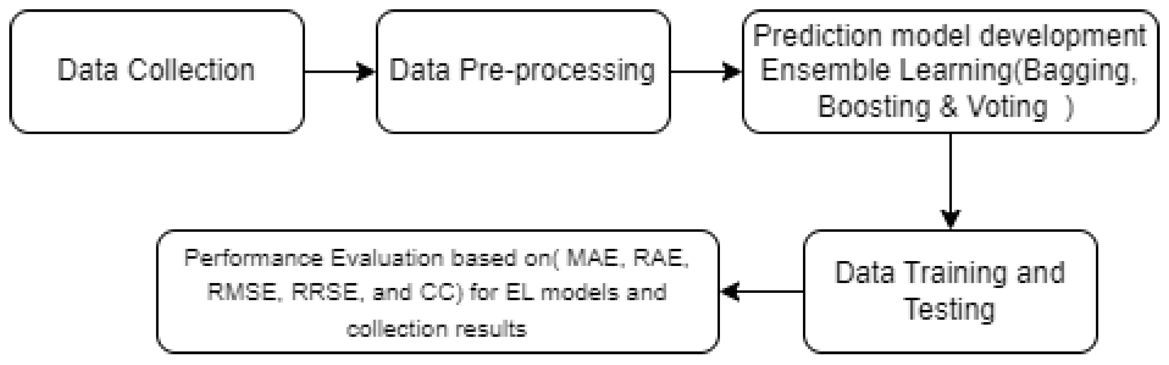
Figure 3.
Algorithm PCA-ComImp
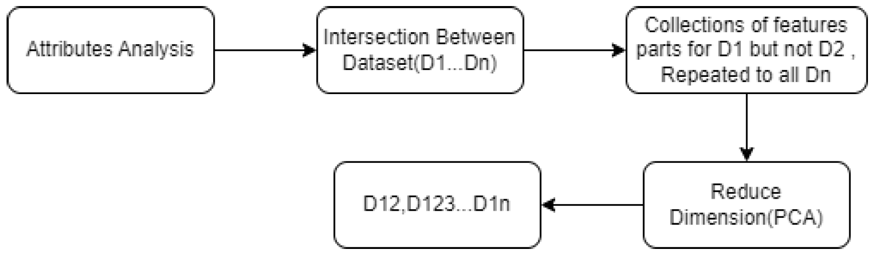
Figure 4.
PCA-ComImp for merge datasets
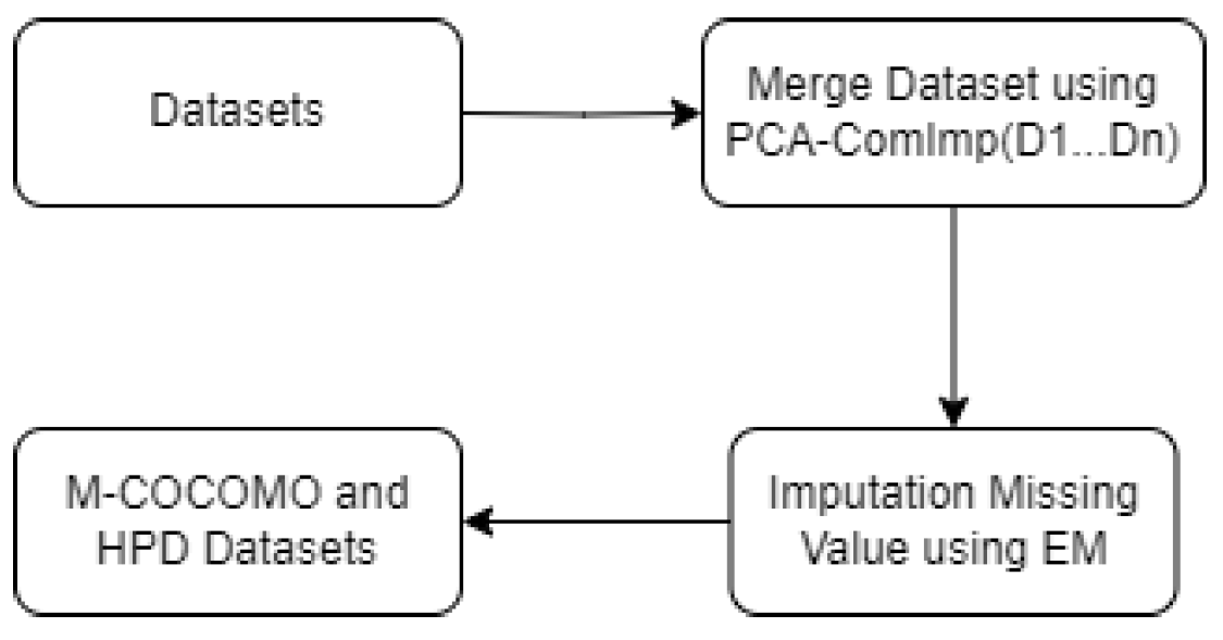
Figure 5.
The COCOMO81 dataset just before standardization
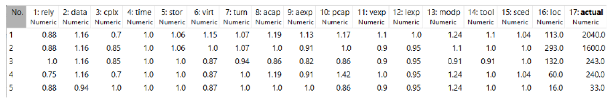
Figure 6.
The COCOMO81 dataset just after standardization
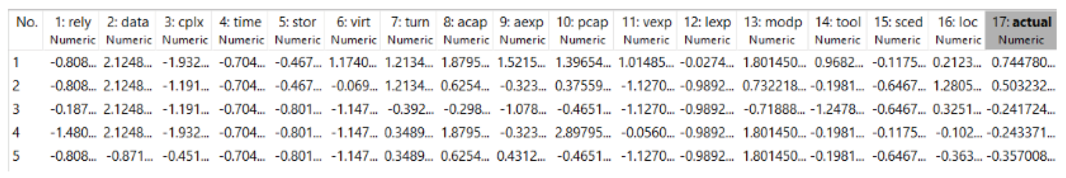
Table 1.
Datasets used in this research
| Dataset name | Source Repository | Number of Features | Number of projects | Output feature-effort | Reference |
| COCOMO81 | Promise | 17 | 63 | Person-months | [1,4,6,11,12,14] |
| COCOMO NASA 1 | Promise | 17 | 63 | Person-months | [1,2,4,16,19] |
| COCOMO NASA 2 | Promise | 24 | 93 | Person-months | [1,5,17] |
| Maxwell | Github | 27 | 62 | Person-hours | [20] |
| Desharnais | Github | 9 | 81 | Person-hours | [8,14,15,18,20,23] |
| Desharnais-1-1 | Github | 12 | 81 | Person-hours | [8] |
| China | Github | 16 | 499 | Person-hours | [9] |
| Albrecht | Github | 8 | 24 | Person-hours | [4,19,21] |
| belady | Github | 2 | 32 | Person-hours | [25] |
| boehm | Github | 2 | 62 | Person-hours | [25] |
| Kitchenham | Github | 4 | 145 | Person-hours | [24] |
Table 2.
A brief description of the COCOMO81 dataset
| COCOMO81 Features | Description | FS | Data Type |
| Rely | Describes the application and its reliability required. | Numeric | |
| Data | Describes the dimension of the database’s records. | ✓ | Numeric |
| IntComplx | Describes the procedure’s complexities. | Numeric | |
| Time | Describes the central processing unit (CPU) time constraint. | ✓ | Numeric |
| Stor | Describes the CPU’s main limitation. | ✓ | Numeric |
| Virt | Describes the machine volatility. | Numeric | |
| Turn | Describes how long it takes to turn around. | Numeric | |
| Acap | Describes the Capability Analyzer. | Numeric | |
| aexp | Describes the app’s experiences. | Numeric | |
| Pcap | Describes programmers’ abilities. | Numeric | |
| vepx | Describes a virtual usage of computers. | Numeric | |
| lexp | Describes the foreign language experience of learning. | Numeric | |
| Modp | Describes the processes utilized in modern software. | Numeric | |
| Tool | Describes the software tools that are implemented. | ✓ | Numeric |
| Sced | Describe the timetable restriction. | Numeric | |
| loc | Describes the source code lines. | ✓ | Numeric |
| Effort | Describes the actual time spent in "person-months". | ✓ | Numeric |
Table 3.
A brief description of the COCOMONasa I dataset
| COCOMO Nasa-I Features | Description | FS | Data Type |
| Rely | Describes the application and its reliability required. | Numeric | |
| Data | Describes the dimension of the database’s records. | ✓ | Numeric |
| IntComplx | Describes the procedure’s complexities. | Numeric | |
| Time | Describes the central processing unit (CPU) time constraint. | ✓ | Numeric |
| Stor | Describes the CPU’s main limitation. | ✓ | Numeric |
| Virt | Describes the machine volatility. | Numeric | |
| Turn | Describes how long it takes to turn around. | Numeric | |
| Acap | Describes the Capability Analyzer. | Numeric | |
| aexp | Describes the app’s experiences. | Numeric | |
| Pcap | Describes programmers’ abilities. | Numeric | |
| vepx | Describes a virtual usage of computers. | Numeric | |
| lexp | Describes the foreign language experience of learning. | Numeric | |
| Modp | Describes the processes utilized in modern software. | Numeric | |
| Tool | Describes the software tools that are implemented. | ✓ | Numeric |
| Sced | Describe the timetable restriction. | Numeric | |
| loc | Describes the source code lines. | ✓ | Numeric |
| Effort | Describes the actual time spent in "person-months". | ✓ | Numeric |
Table 4.
A brief description of the COCOMONasa II dataset
| COCOMO Nasa-II Features | Description | FS | Data Type |
| id | Describes the Project ID. | Numeric | |
| ProjectNam | Describes the Project name. | Ordinal | |
| mode | Describes the development mode. | Ordinal | |
| year | Describes the year of development. | Numeric | |
| cat2 | Describes the category of application. | Ordinal | |
| center | Describes which NASA center. | Ordinal | |
| forg | Describes the flight or ground system. | Ordinal | |
| Rely | Describes the application and its reliability required. | Numeric | |
| Data | Describes the dimension of the database’s records. | ✓ | Numeric |
| IntComplx | Describes the procedure’s complexities. | Numeric | |
| Time | Describes the central processing unit (CPU) time constraint. | ✓ | Numeric |
| Stor | Describes the CPU’s main limitation. | ✓ | Numeric |
| Virt | Describes the machine volatility. | Numeric | |
| Turn | Describes how long it takes to turn around. | Numeric | |
| Acap | Describes the Capability Analyzer. | Numeric | |
| aexp | Describes the app’s experiences. | Numeric | |
| Pcap | Describes programmers’ abilities. | Numeric | |
| vepx | Describes a virtual usage of computers. | Numeric | |
| lexp | Describes the foreign language experience of learning. | Numeric | |
| Modp | Describes the processes utilized in modern software. | Numeric | |
| Tool | Describes the software tools that are implemented. | ✓ | Numeric |
| Sced | Describe the timetable restriction. | Numeric | |
| loc | Describes the source code lines. | ✓ | Numeric |
| Effort | Describes the actual time spent in "person-months". | ✓ | Numeric |
Table 5.
A brief description of the KITCHENHAM dataset
| KITCHENHAM Features | Description | FS | Data Type |
| Actual. duration | Describes the project duration. | Numeric | |
| Adjusted function points | Describes the Function Point Adjustment Factor. | Numeric | |
| First. Estimate | Describes the first estimate for the project. | ✓ | Numeric |
| Actual. effort | Describes the actual time spent in "person-hours". | ✓ | Numeric |
Table 6.
A brief description of the DESHARNAIS dataset
| DESHARNAIS Features | Description | FS | Data Type |
| TeamExp | Describes the project’s team member’s capabilities. | Numeric | |
| ManagerExp | Describes the project manager’s experience. | Numeric | |
| YearEnd | Describes the final year of the project. | Numeric | |
| Transactions | Describes the number of transactions processed. | ✓ | Numeric |
| Entities | Describes the overall number of instances in the structure’s data. | Numeric | |
| PointsAdjust | Describe the adjustments functionality points. | ✓ | Numeric |
| Envergure | Describes the environment for the project. | Numeric | |
| Language | Describes the project’s language. | Ordinal | |
| Effort | Describes the actual time spent in "person-hours". | ✓ | Numeric |
Table 7.
A brief description of the DESHARNAIS_1_1 dataset
| DESHARNAIS_1_1 Features | Description | FS | Data Type |
| ID | Describes the object ID. | Numeric | |
| TeamExp | Describes the project’s team member’s capabilities. | Numeric | |
| ManagerExp | Describes the project manager’s experience. | Numeric | |
| YearEnd | Describes the final year of the project. | Numeric | |
| Transactions | Describes the number of transactions processed. | ✓ | Numeric |
| Entities | Describes the overall number of instances in the structure’s data. | Numeric | |
| PointsAdjust | Describe the adjustments functionality points. | ✓ | Numeric |
| PointsnonAdjust | Describes the non-adjustment function points(Transaction & Entities). | ✓ | Numeric |
| Length | Describes the actual project schedule in months. | Numeric | |
| Language | Describes the language used for the project. | Ordinal | |
| Adjustment | Describes the function point adjustment factor for complexity. | Numeric | |
| Effort | Describes the actual time spent in "person-hours". | ✓ | Numeric |
Table 8.
A brief description of the MAXWELL dataset
| MAXWELL Features | Description | FS | Data Type |
| Size | Describes the application size. | ✓ | Numeric |
| Duration | Describes the project duration. | ✓ | Numeric |
| Time | Describes the Time taken. | Numeric | |
| Year | Describes the year of development. | Numeric | |
| app | Describes the application type for the project. | Numeric | |
| har | Describes the required hardware framework. | Numeric | |
| dba | Describes the project’s database. | Numeric | |
| ifc | Describes the user interface for the project. | Numeric | |
| Source | Describes the conditions under which software is created. | Numeric | |
| nlan | Describes the number of languages that were used. | Numeric | |
| telonuse | Describes the Telon used for the project. | Numeric | |
| T01 | Describes how the client interacts. | Numeric | |
| T02 | Describes the creation of an environment’s capability. | Numeric | |
| T03 | Describes the project’s workforce accessibility. | Numeric | |
| T04 | Describes the standard used for the project. | Numeric | |
| T05 | Describes the method used for the project. | Numeric | |
| T06 | Describes the tools used for the project. | Numeric | |
| T07 | Describes the logic that underlies the complexity of the software. | Numeric | |
| T08 | Describes the range of limitations. | Numeric | |
| T09 | Describes the standard of excellence criteria. | Numeric | |
| T10 | Describes what is necessary for productivity. | Numeric | |
| T11 | Describes the process of installation criteria. | Numeric | |
| T12 | Describes the critical thinking skills of the team members. | Numeric | |
| T13 | Describes the program and the experience of staff members. | Numeric | |
| T14 | Describes the project’s team technical capabilities. | Numeric | |
| T15 | Describes the project’s team member’s capabilities. | ✓ | Numeric |
| Effort | Describes the actual time spent in "person-hours". | ✓ | Numeric |
Table 9.
A brief description of the BELADY dataset
| BELADY Features | Description | FS | Data Type |
| Size | Describes the application size. | ✓ | Numeric |
| Effort | Describes the actual time spent in "person-hours". | ✓ | Numeric |
Table 10.
A brief description of the BOEHM dataset
| BOEHM Features | Description | FS | Data Type |
| Size | Describes the application size. | ✓ | Numeric |
| Effort | Describes the actual time spent in "person-hours". | ✓ | Numeric |
Table 11.
A brief description of the CHINA dataset
| CHINA Features | Description | FS | Data Type |
| AFP | Describe the altered functionality parameters. | Numeric | |
| Input | Describes the function points of input for the project. | Numeric | |
| Output | Describes the function points of output for the project. | Numeric | |
| Inquiry | Describes the function points of external output inquiry. | Numeric | |
| Files | Describes the function pointers of internal logical files. | Numeric | |
| Interface | Describes the function pointers of the external interface added. | Numeric | |
| Added | Describes the function pointers of the added functions. | Numeric | |
| Changed | Describes the function pointers of changed functions. | Numeric | |
| Resource | Describes the team type for the project. | ✓ | Numeric |
| Duration | Describes the project duration. | Numeric | |
| PDR_AFP | Describes the Productivity delivery rate(adjustment functionality parameters). | Numeric | |
| PDR _UFP | Describes the Productivity delivery rate(Un-adjustment functionality parameters). | Numeric | |
| NPDR _AFP | Describes the Normalized productivity delivery rate(adjustment functionality parameters). | Numeric | |
| NPDU _UFP | Describes the Productivity delivery rate(Un-adjustment functionality parameters). | Numeric | |
| N-Effort | Describes the normalized effort. | ✓ | Numeric |
| Effort | Describes the actual time spent in "person-hours". | ✓ | Numeric |
Table 12.
A brief description of the ALBRECHT dataset
| ALBRECHT Features | Description | FS | Data Type |
| Input | Describes the quantity of inputs a software must handle. | Numeric | |
| Output | Describes the quantity of outputs that a program generates. | ✓ | Numeric |
| Inquiry | Describes the number of queries or questions that an application must respond to. | ✓ | Numeric |
| Files | Describes the amount of records needed for the program to write to or read from. | Numeric | |
| FPAdj | Describes the Function Point Adjustment Factor. | Numeric | |
| RawFPcounts | Describes the Function Point Measures are used to calculate the raw function points. | ✓ | Numeric |
| AdjFP | Describes the function’s point adjustments factor given by the original function points. | ✓ | Numeric |
| Effort | Describes the actual time spent in "person-hours". | ✓ | Numeric |
Table 13.
A brief description of the M-COCOMO dataset after feature selection
| M-COCOMO Features | Description | Data Type |
| Data | Describes the Database Size. | Numeric |
| Time | Describes the CPU time limitation. | Numeric |
| Stor | Describes the CPU’s main limitation. | Numeric |
| Tool | Describes the software tools that are implemented. | Numeric |
| loc | Describes the source code lines. | Numeric |
| Effort | Describes the actual time spent in "person-months". | Numeric |
Table 14.
A brief description of the HPD dataset after feature selection
| HPD Features | Description | Data Type |
| Resource | Describe the team type for the project. | Numeric |
| Output | Describes the quantity of outputs that a program generates. | Numeric |
| Enquiry | Describes the number of queries or questions that an application must respond to. | Numeric |
| Team Exp | Describes the team experience in years. | Numeric |
| First Estimate | Describes the first estimate for the project. | Numeric |
| AFP | Describes the Function Point Adjustment Factor | Numeric |
| Non-AFP | Describes the non-adjustment function points. | Numeric |
| Transaction | Describes the number of transactions processed. | Numeric |
| Size | Describes the application size. | Numeric |
| Duration | Describes the project duration. | Numeric |
| N-effort | Describes the normalized effort. | Numeric |
| Effort | Describes the actual time spent in "person-hours". | Numeric |
Table 15.
A brief description of the M-COCOMO dataset after PCA-ComImp
| M-COCOMO Features | Description | Data Type |
| Rely | Describes the application and its reliability required. | Numeric |
| Data | Describes the dimension of the database’s records. | Numeric |
| IntComplx | Describes the procedure’s complexities. | Numeric |
| Time | Describes the central processing unit (CPU) time constraint. | Numeric |
| Stor | Describes the CPU’s main limitation. | Numeric |
| Virt | Describes the machine volatility. | Numeric |
| Turn | Describes how long it takes to turn around. | Numeric |
| Acap | Describes the Capability Analyzer. | Numeric |
| aexp | Describes the app’s experiences. | Numeric |
| Pcap | Describes programmers’ abilities. | Numeric |
| vepx | Describes a virtual usage of computers. | Numeric |
| lexp | Describes the foreign language experience of learning. | Numeric |
| Modp | Describes the processes utilized in modern software. | Numeric |
| Tool | Describes the software tools that are implemented. | Numeric |
| Sced | Describes the timetable constraint . | Numeric |
| loc | Describes the source code lines. | Numeric |
| Effort | Describes the actual time spent in "person-months". | Numeric |
Table 16.
A brief description of the HPD dataset after PCA-ComImp
| HPD Features | Description | Data Type |
| Input | Describes the quantity of inputs a software must handle. | Numeric |
| Output | Describes the quantity of outputs that a program generates. | Numeric |
| File | Describes the number of files required for a program to write to or read from. | Numeric |
| First Estimate | Describes the first estimate for the project. | Numeric |
| AFP | Describe the function of the Points Adjustments Factor. | Numeric |
| N-effort | Describes the normalized effort. | Numeric |
| Effort | Describes the actual time spent in "person-hours". | Numeric |
Table 17.
Comparison of EL models with COCOMO81 Dataset
| Model | MAE | RMSE | RAE | RRSE | CC |
| Bagging | 0.0158 | 0.0671 | 53.2419 % | 56.3547 % | 0.9578 |
| AdaBoost | 0.0159 | 0.0589 | 46.9494 % | 48.5212 % | 0.9998 |
| Voting | 0.0143 | 0.0565 | 44.3188 % | 44.5415 % | 0.9998 |
Table 18.
Comparison of EL with COCOMONasa I Dataset
| Model | MAE | RMSE | RAE | RRSE | CC |
| Bagging | 0.0214 | 0.0819 | 53.6069 % | 58.0754 % | 0.9759 |
| AdaBoost | 0.0039 | 0.0356 | 9.7092 % | 25.2217 % | 0.9996 |
| Voting | 0.0168 | 0.0640 | 42.0561 % | 45.3716 % | 0.9995 |
Table 19.
Comparison of EL with COCOMONasa II Dataset
| Model | MAE | RMSE | RAE | RRSE | CC |
| Bagging | 0.0143 | 0.0661 | 53.8579 % | 57.3016 % | 0.9578 |
| AdaBoost | 0.0013 | 0.0228 | 5.5397 % | 19.7348 % | 0.9998 |
| Voting | 0.0109 | 0.0502 | 40.9738 % | 43.5082 % | 0.9998 |
Table 20.
Comparison of EL with Desharnais Dataset
| Model | MAE | RMSE | RAE | RRSE | CC |
| Bagging | 0.0131 | 0.0615 | 53.5125 % | 55.7224 % | 0.9179 |
| AdaBoost | 0.009 | 0.0419 | 36.7875 % | 37.9658 % | 0.9999 |
| Voting | 0.0115 | 0.0519 | 47.0259 % | 47.0276 % | 0.9999 |
Table 21.
Comparison of EL with Desharnais_1_1 Dataset
| Model | MAE | RMSE | RAE | RRSE | CC |
| Bagging | 0.0094 | 0.0454 | 36.6104 % | 40.0959 % | 0.9164 |
| AdaBoost | 0.0094 | 0.0421 | 36.7417 % | 37.1824 % | 0.9999 |
| Voting | 0.0102 | 0.0463 | 41.9686 % | 41.9719 % | 0.9999 |
Table 22.
Comparison of EL with Belady Dataset
| Model | MAE | RMSE | RAE | RRSE | CC |
| Bagging | 0.0347 | 0.102 | 55.6538 % | 57.7707 % | 0.8922 |
| AdaBoost | 0.0023 | 0.0313 | 3.6618 % | 17.7461 % | 0.9996 |
| Voting | 0.0305 | 0.0878 | 48.8484 % | 49.7202 % | 0.9996 |
Table 23.
Comparison of EL with Boehm Dataset
| Model | MAE | RMSE | RAE | RRSE | CC |
| Bagging | 0.0182 | 0.0771 | 56.4441 % | 60.7297 % | 0.8685 |
| AdaBoost | 0.00643 | 0.0488 | 19.7554 % | 38.4640 % | 0.9989 |
| Voting | 0.0176 | 0.0727 | 54.4594 % | 57.2534 % | 0.9989 |
Table 24.
Comparison of EL with Kitchenham Dataset
| Model | MAE | RMSE | RAE | RRSE | CC |
| Bagging | 0.0076 | 0.0467 | 53.5633 % | 55.4589 % | 0.9936 |
| AdaBoost | 0.0003 | 0.0101 | 1.9578 % | 12.0124 % | 0.9999 |
| Voting | 0.0071 | 0.0423 | 49.8529 % | 50.2115 % | 0.9999 |
Table 25.
Comparison of EL with Maxwell Dataset
| Model | MAE | RMSE | RAE | RRSE | CC |
| Bagging | 0.0172 | 0.0705 | 54.0836 % | 55.9919 % | 0.9615 |
| AdaBoost | 0.0118 | 0.0481 | 37.2787 % | 38.1860 % | 0.9999 |
| Voting | 0.0140 | 0.0556 | 44.0882 % | 44.1649 % | 0.9999 |
Table 26.
Comparison of EL with Albrecht Dataset
| Model | MAE | RMSE | RAE | RRSE | CC |
| Bagging | 0.0429 | 0.1116 | 53.7217 % | 55.6905 % | 0.9892 |
| AdaBoost | 0.0299 | 0.0764 | 37.3913 % | 38.2528 % | 0.9999 |
| Voting | 0.0202 | 0.0505 | 25.2501 % | 25.2845 % | 0.9999 |
Table 27.
Comparison of EL with China Dataset
| Model | MAE | RMSE | RAE | RRSE | CC |
| Bagging | 0.0015 | 0.0183 | 36.1662 % | 40.3380 % | 0.9938 |
| AdaBoost | 0.0001 | 0.0051 | 1.4717 % | 11.1515 % | 0.9998 |
| Voting | 0.0021 | 0.0229 | 49.9593 % | 50.2752 % | 0.9998 |
Table 28.
Comparison of EL for the M-COCOMO Dataset
| ComImp | Model | MAE | RMSE | RAE | RRSE | CC |
| Bagging | 0.0066 | 0.0443 | 43.5009 % | 49.6498 % | 0.9320 | |
| AdaBoost | 0.0009 | 0.0183 | 6.1038 % | 20.948 % | 0.9999 | |
| Voting | 0.0057 | 0.0357 | 37.3736 % | 40.9089 % | 0.9999 | |
| PCA-ComImp | Bagging | 0.0069 | 0.0429 | 45.1777 % | 49.1607 % | 0.9359 |
| AdaBoost | 0.0002 | 0.0085 | 1.0243 % | 9.7135 % | 0.9999 | |
| Voting | 0.0038 | 0.0276 | 24.801 % | 31.697 % | 0.9999 |
Table 29.
Comparison of EL with HPD Dataset
| ComImp | Model | MAE | RMSE | RAE | RRSE | CC |
| Bagging | 0.0008 | 0.0135 | 36.2509 % | 39.5167 % | 0.9978 | |
| AdaBoost | 0.0122 | 0.0494 | 37.2849 % | 38.5657 % | 0.9997 | |
| Voting | 0.0004 | 0.0054 | 15.6635 % | 15.6637 % | 0.9999 | |
| PCA-ComImp | Bagging | 0.0008 | 0.0135 | 36.0581 % | 39.5376 % | 0.9972 |
| AdaBoost | 0.0001 | 0.0002 | 1.5617 % | 10.1143 % | 0.9999 | |
| Voting | 0.0008 | 0.0114 | 32.986 % | 33.1954 % | 0.9999 |
Disclaimer/Publisher’s Note: The statements, opinions and data contained in all publications are solely those of the individual author(s) and contributor(s) and not of MDPI and/or the editor(s). MDPI and/or the editor(s) disclaim responsibility for any injury to people or property resulting from any ideas, methods, instructions or products referred to in the content. |
© 2024 by the authors. Licensee MDPI, Basel, Switzerland. This article is an open access article distributed under the terms and conditions of the Creative Commons Attribution (CC BY) license (http://creativecommons.org/licenses/by/4.0/).
Copyright: This open access article is published under a Creative Commons CC BY 4.0 license, which permit the free download, distribution, and reuse, provided that the author and preprint are cited in any reuse.


