Checking the 8Be Anomaly with a Two-Arm Electron Positron Pair Spectrometer

Preprint

Article

Checking the ⁸Be Anomaly with a Two-Arm Electron Positron Pair Spectrometer

Altmetrics

Downloads

109

Views

Comments

A peer-reviewed article of this preprint also exists.

Supplementary Material

supplementary.pdf (442.79KB )

Submitted:

05 March 2024

Posted:

05 March 2024

You are already at the latest version

Alerts

Abstract

We have repeated the experiment performed recently by Krasznahorkay et al., (Phys. Rev. Lett. 116, 042501 (2016)), which may indicate a new particle called X17 in the literature. In order to get a reliable, and independent result, we used a different type of electron-positron pair spectrometer which have a more simple acceptance/efficiency as a function of the correlation angle, but the other conditions of the experiment were very similar to the published ones. We could confirm the presence of the anomaly measured at the Ex=18.15 MeV resonance, and also confirm their absence at the Ex=17.6 MeV resonance, and at Ep= 800 keV off resonance energies.

Keywords:

Subject: Physical Sciences - Nuclear and High Energy Physics

1. Introduction

An experiment was conducted at the ATOMKI Laboratory (Debrecen, Hungary) [1] in 2016, studying the

{}^{7}{Li}

(p,

e^{+}

e^{-}

)

{}^{8}{Be}

nuclear reaction. The target nucleus was excited through proton capture, with the experiment set up to detect

e^{+}

e^{-}

pairs produced in the Internal Pair Creation (IPC) during the transition from the excited to the ground state of

{}^{8}{Be}

. The experimental setup was using a set of multiwire proportional counters placed in front of

Δ

E and E detectors, to determine the

e^{+}

e^{-}

opening angle,

θ (e^{+} e^{-})

. The very thin

Δ

E detectors were made of plastic scintillators and chosen to provide excellent gamma suppression. While the much thicker E detectors were used to measure the total energy of the electron and positron. A detailed description of the experimental setup can be found in [2]. The ATOMKI collaboration observed a deviation in the

θ (e^{+} e^{-})

distribution with respect to the expected Rose theory distribution [3], at around 140 degrees.

Zhang and Miller [4] studied the protophobic vector boson explanation in

{}^{8}{Be}

, by deriving an isospin relation between the coupling of photon and X17 to nucleons. They are expected to have contributions from M1 multipolarity transitions coming from the resonant proton capture (17.6 and 18.15 MeV

J^{π} = 1^{+}

states) as well as from the E1 multipolarity transitions resulting from the direct proton-capture process.

After 2016 the ATOMKI collaboration repeated the measurements, while improving the experimental setup in many different ways [5,6]. The anomaly kept appearing in the follow-up experiments, with no nuclear physics model being able to explain it. This led to the explanation of a new particle, beyond the Standard Model of particle physics, created and decaying to

e^{+}

e^{-}

pairs, being detected in these experiments. The hypothetical particle is now commonly referred to as X17, because of the invariant mass calculated from the

e^{+}

e^{-}

anomalies.

In addition to the

{}^{7}{Li}

(p,

e^{+}

e^{-}

)

{}^{8}{Be}

nuclear reaction, since 2019, the same collaboration has also studied the

{}^{3}H

(p,

e^{+}

e^{-}

)

{}^{4}{He}

[5] and

{}^{11}B

(p,

e^{+}

e^{-}

)

{}^{12}C

[6] reactions. Different proton energies were used, leading to anomalies appearing in the

θ (e^{+} e^{-})

distributions at different angles. All well consistent with the assumption of an

m_{X} \approx

17 MeV particle being created with different kinetic energies, leading to different opening angles between the electron positron pairs.

The ATOMKI anomaly, being a genuine physics effect, is supported by a number of arguments.

The anomaly has been observed in ${}^{8}{Be}$ with experimental setups using different geometries, with 5 and 6 arm spectrometers [7].
The anomaly has been observed using a fundamentally different position sensitive detectors: multi-wire chambers and silicon strip detectors [1,7].
The anomaly has been observed in three different nuclei by now ( ${}^{9}{Be}$ , ${}^{4}{He}$ and ${}^{12}C$ ), showing up at $e^{+}$ $e^{-}$ opening angles consistent with a single particle [1,5,6].
The anomaly has been observed at different proton beam energies at varying $e^{+}$ $e^{-}$ opening angles, also consistent with a single particle [1,5,6].
All observed anomalies have a very high statistical significance such as 6.8 $σ$ [1], $6.6 - 8.9 σ$ [5], and $3 - 8 σ$ [6]..

Despite the consistency of the numerous observations at ATOMKI, more experimental data is needed to understand the nature of this anomaly. Many experiments around the world started looking for such a particle in different channels, or are planning to do so. Many of these experiments [8,9,10,11] already put constraints on the coupling of such a hypothetical particle with ordinary matter. Others are still in an R&D phase, soon to contribute to a deeper understanding of this phenomenon as concluded by the community report of the Frascati conference [8]. Such a report also gives a nice overview of the possible theoretical interpretation of the observed anomalies in

{}^{8}{Be}

{}^{4}{He}

, and

{}^{12}C

[8].

At the VNU University of Science (HUS), we have a 5SDH-2 Pelletron accelerator, a 1.7 MV tandem electrostatic type. It can provide a proton beam with energy from 0.35 to 3.4 MeV or 0.7-5.1 MeV for the alpha beam. The accelerator was installed and operated in 2011 [12], and some initial work for the research in nuclear reaction cross-sections has been done [13]. This article aims to look for the 8Be anomaly at the VNU University of Science (HUS) with a two-arm electron-positron spectrometer specifically designed and built for this purpose.

2. Experimental Methods

In order to make our experimental results easier to reproduce, in the first part of this paper, we give a more precise description of our

e^{+} e^{-}

pair spectrometer with the setup of the detectors and the electronics connected to them. This will be followed by a brief description of the data acquisition system and the results of testing and calibrating the detectors.

2.1. The $e^{+}$ $e^{-}$ Spectrometer

In the present experiment, two detector telescopes, including Double Silicon Strip Detectors (DSSD) and plastic scintillators were used, placed at an angle of

140^{°}

with respect to each other. The diameter of the carbon fiber tube of the target chamber has been reduced from 70 mm (used in ATOMKI) to 48 mm to allow a closer placement of the telescopes to the target. This way, we could cover a similar solid angle at

140^{°}

like the one used in the ATOMKI experiment Figure 1.

In this setup, the efficiency function has only one maximum as a function of the

e^{+} e^{-}

opening angle. This angular dependence can be simulated and calibrated more robustly than for more complicated configurations. Another advantage of this setup that we used is that its sensitivity to background from cosmic radiation is significantly less.

The two detector telescopes were placed at azimuthal angles −20° and −160° with respect to horizontal. This meant that cosmic rays, predominantly arriving vertically, would have a very low chance of hitting both telescopes at the same time.

For the detection of 1-20 MeV

e^{+}

and

e^{-}

particles, which are considered high-energy in nuclear physics, Geant4 [14] calculations were performed for different detector materials. This included plastic scintillators, Ge semiconductor detectors, and LaBr₃ scintillators. Much better energy resolution could be achieved with the latter two types of detectors than with a plastic scintillator. The FWHM at 17.6 MeV can be achieved below 20 keV for the Ge detector and 150 keV for the LaBr3 detector. However, our simulations also showed that in the case of high-density and high Z detectors, the efficiency of the total energy detection in the energy response function is greatly reduced compared to the integral of the response function. The ratio between full energy events and total recorded events is smaller than 1.5% at electrons energy of 18 MeV for 3x3 inches LaBr₃ detector. In materials with higher atomic numbers, the

e^{+}

and

e^{-}

particles slow down faster, and thus, the probability of generating bremsstrahlung radiation is higher. However, there is a high probability that these radiations will escape the detector. This is why the probability of detecting

e^{+}

and

e^{-}

particles at full energy is reduced in these high Z materials. Therefore, we used special plastic scintillators for this task. The dimensions of the EJ200 plastic scintillators were chosen (82 × 82 × 80 mm³ each) in such the way that these high-energy particles would be completely stopped in them.

To collect the light generated by the

e^{+}

e^{-}

particles slowing down in the detector from all corners with the same efficiency, the SCIONIX company provided the detector with specially shaped light guides. The surfaces of both the detectors and the light guides were diamond polished. The collected light was converted to an electronic signal by Hamamatsu photomultiplier tube (PMT) type R594 assemblies.

The time resolution of the detector turned out to be adequate despite the large size of the detector and multiple light reflections inside. It was measured with a

{}^{60}{Co}

source between 2 detectors, and found to be less than 1 ns, as shown in Figure 2.

In the absence of a high-energy electron source, the energy resolution of the detector could only be determined with the help of

e^{+}

e^{-}

pairs from internal pair creation. We will come back to this in section 2.4 in connection with the energy calibration of the detectors.

Double-sided Silicon Strip Detectors (DSSD), W1(DS)-500, were used to measure the energy loss of the

e^{+} e^{-}

particles and their directions. The DSSDs were purchased from Micron Semiconductor. They consist of 16 sensitive strips on the junction side and 16 orthogonal strips on the ohmic side. Their element pitch is 3.01 mm for a total coverage of 49.5 x 49.5 mm². They are mounted on a printed circuit board (PCB), with 34 pins on one edge for their readout. These are connected via 34-conductor flat cables to the pre-amp boxes.

Mesytec MUX32 type 32-channel preamplifiers, linear amplifiers, timing filter amplifiers, timing discriminators and multiplexers were used. The full width of the 5^th-order shaped energy signals is 1.5

μ

s, and the full rate capability of the MUX32 unit is 800 kHz. The energy resolution of the channels is 5.5 keV Si + 0.064 keV/pF. The timing filter amplifier signals are shaped with 20 ns integration time and 100 ns differentiation time, followed by leading edge discriminators. It is a very fast multiplexed preamplifier, shaper, and discriminator combination with very good energy and timing resolutions. The MUX-32 consists of two MUX-16s; each MUX-16 manages 16 inputs, up to two simultaneous responding channels are identified, and two amplitudes plus the two corresponding amplitude-coded addresses (position signals) are sent to the outputs. Therefore, it can manage the double-hit events with full energy and position information in the x and y directions. These modules are especially well-suited for DSSD detectors.

By properly shielding and grounding the detectors, using 10

μ

m thick Al foils mounted on PCBs both at the front and the back side of the detectors and shielding the flat cables and connectors, we managed to reduce their electronic noise and could lower the levels of the discriminators below 50 keV. For simplicity, the detectors are operated in air without dedicated cooling. The first test and calibration of the detectors were performed with a mixed

α

-source containing

{}^{239}{Pu}

{}^{244}{Cm}

, and

{}^{241}{Am}

. The experimental configuration was used in Geant4 simulation code [14]. All materials used to construct the experiment have been included in the simulation geometry. Therefore, the energy loss in the Al foil and in the air (5 mm) were taken into account.

2.2. Data acquisition system

The data acquisition system uses Versa Module Eurocard (VME), Analog-to-Digital Converter (ADC), Time-to-Digital Converter (TDC), and Charge-to-Digital Converter (QDC) units, which were read out with the help of a commodity desktop PC. The software used for configuring the VME devices and recording the data collected can be found in [15].

Constant Fraction Discriminators (CFDs) and TDC units were used to determine the arrival time of the signals coming from the plastic scintillators, and QDCs were used to digitize their energy signals. The block diagram of the electronics connected to the detectors is shown in Figure 3. The signals received from the MUX32 multiplexer were digitized with the help of ADC and TDC units.

2.3. Calibration of the DSSD Detectors

The energy measured by the DSSD was calibrated using information from the

e^{+}

e^{-}

particles, which were produced by the

{}^{7}{Li}

(p,

γ

)

{}^{8}{Be}

nuclear reaction. The energy of the bombarding protons was set to the E_p=441 keV resonance. When creating the spectrum, we required real coincidence between the DSSD detector and the plastic scintillator located behind it by requiring the time different between two plastics is smaller than 40 ns. The two plastics measured the total energy of the

e^{+}

e^{-}

particles. We also required this energy to be in the 6-20 MeV range. The experimental configuration was used in Geant4 simulation code [14]. Figure 4 shows the energy loss distribution of electrons and positrons passing through one of the DSSD detectors. The histograms show reasonably good agreement between the experimental and simulated distributions, however we obtained some differences around 100 keV and 350 keV. The former can be caused by some electronic noise, while the latter is caused by the events when both the

e^{+}

and

e^{-}

created during the internal pair production passed through the same DSSD detector. The detection efficiency with a CFD threshold of 50 keV was greater than 97% for electrons and positrons.

The histograms in Figure 5 show the (non calibrated) distribution of the x and y coordinates of the impact points of the

e^{+}

e^{-}

particles that hit the DSSD detector. The peaks of the fence spectrum correspond to the coordinates of particles passing through the individual silicon strips. As shown, the assignment of the recorded data to the x and y strips is very clear. The width of DSSD was used to convert the recorded data to position in cm scale with origin at the center (two dimension plot in Figure 5). Of the 70,000 events recorded for these distributions, only around 3% of events had to be excluded due to missing information in either the x or y direction.

2.4. Calibration of the Scintillation Detectors

The energy distribution of the electrons and positrons in internal pair creation individually is contiguous. However, if the electron and positron lose their energy in the same detector, the energy distribution of such events will show peaks at the transition energies -

2 m_{e} c^{2}

. The scintillator detectors were calibrated using such events. If the detectors are close enough to the target, there is a high probability of the above internal energy summing. The energy spectrum measured by the scintillators for events selected by gating on double-hit in the DSSD detector, can be found in Figure 6.

3. Experimental Results

The experiments were performed in Hanoi (Vietnam) at the 1.7 MV Tandem accelerator of HUS, with different proton beam energies between 0.4

\leq E_{p} \leq 1.3

MeV. The typical beam currents for these experiments were from 1 to 1.5

μ

LiF targets with thicknesses of ≈30

μ

g/cm² evaporated onto 10

μ

m thick Al foils, as well as Li₂O targets with thicknesses of ≈0.3 mg/cm², were used on 1

μ

m thick Ni foils in order to maximize the yield of the

e^{+} e^{-}

pairs. The LiF is a more stable target, and it is easy to evaporate. That was the reason we used it at low bombarding energy (E_p=441 keV, E_x=17.6 MeV) to calibrate the spectrometer. However, if we increase the beam energy from 441 keV (E_x= 17.6 MeV) to 1.04 MeV (E_x=18.15 MeV), the cross-section of the

{}^{19}F

(p,

α

)

{}^{16}O

reaction increases very fast and the created

e^{+}

e^{-}

pairs coming from the decay of the 6.05 MeV E₀ transition would overload our electronics and data acquisition, and observing

e^{+}

e^{-}

pairs from the 18.15 MeV transition would not be feasible.

γ

radiations were detected by a 3”x3” NaI(Tl) detector monitoring also any potential target losses. The detector was placed at a distance of 25 cm from the target at an angle of 90 degrees to the beam direction.

A single energy spectrum measured by the scintillators and gated by “multiplicity=2” events in the DSSD detector, which means that both the electron and positron coming from the internal pair creation are detected in the same telescope, is shown in Figure 6 for telescope 1. Figure 6 clearly shows the transitions from the decay of the 17.6 MeV resonance state to the ground and first excited states in

{}^{8}{Be}

. The cosmic ray background was already subtracted from that. The energy resolution of the plastic scintillator at 17.6 MeV was extremely good (5.2%), proving the very good light collection from the whole detector. The ‘’background” below the peak comes mostly from the wide (1.5 MeV) transition going to the first excited state of

{}^{8}{Be}

and from the tail of the 17.6 MeV transition. The energy resolution of the 6.05 MeV (

{}^{16}O

) peak is also good.

In order to check the effective thickness of the Li₂O targets, we measured the excitation function of

{}^{8}{Be}

via

{}^{7}{Li}

(p,

γ

)

{}^{8}{Be}

reaction by scanning the proton beam energies from 441 keV to 1300 keV. The events with multiplicity-2 in DSSD and measured energy in the plastic scintillator larger than 10 MeV were counted, and their rate was plotted in Figure 7. Two resonance peaks were observed at the proton beam energies of around 441 and 1040 keV [16,17]. The width of the resonance shows the effect of the target thickness. For the 441 keV resonance, it was found to be approximate 150 keV, which means about 0.44 mg/cm² target thickness, since the energy loss of the protons is 340 keV/mg/cm².

The efficiency (acceptance) as a function of the correlation angle in comparison to isotropic emission was determined from the same data set by using uncorrelated

e^{+}

e^{-}

pairs formed of separate, single events [2]. To do this, uncorrelated

e^{+}

e^{-}

pairs have been recorded during the experiment. The analysis would select event pairs with uncorrelated electrons/positrons hitting different telescopes in the events. The opening angle distribution of electron/positron pairs from such events is shown by the black line in Figure 8 (left). The green line is a simulation curve produced using Geant4. They show quite a good agreement between the estimated experimental and simulation efficiencies.

Coincidence events, with both arms of the spectrometer detecting

e^{+}

e^{-}

particles, were also recorded. The opening angle distribution of

e^{+}

e^{-}

pairs from such events is shown in Figure 8 (right). The cosmic background data had been collected and analyzed similar to the experiment data and subtracted. The total time collection of both data had been normalized.

In the first experiment, we used a proton beam energy of 411 keV to bombard the LiF target. Through this, the

{}^{8}{Be}

nucleus would be created in the 17.6 MeV excited state. Figure 9 shows the angular correlations of

e^{+}

e^{-}

pairs originating from the transition of this 17.6 MeV excited state of

{}^{8}{Be}

to its ground state. The Monte Carlo detector simulations of the experiment were done using Geant4 and are shown as histograms in Figure 9 for M1 (dash-dotted line) and E1 (dotted line) multipolarity transitions. The simulation included the geometries of the target chamber, target backing, and detector arm assemblies. The interaction of generated electrons, positrons, and gamma rays was then simulated with the experimental setup. Internal Pair Creation (IPC) events, generated from both the possible E1 and M1 transitions, were simulated this way. The combination of the E1+M1 distributions shows a good agreement with the experimental data. The dominant M1 part (87.4%) is clearly understood since it is a

1^{+}

–>

0^{+}

transition. The 12.8% E1 mixing can also be understood since the energy loss in the target was about 150 keV, which is about 14 times larger than the width of the resonance (

Γ

=10.7 keV [16], and we integrated a reasonable amount from the proton direct capture part of the excitation function [17] as well, which has a multipolarity of E1.

In the second experiment, we changed the proton beam energy to 800 keV at the off-resonance energies. With the same method to build the total simulation curve and show the experimental data in the Figure 10, we can see the simulated curve go through the middle of data points. There is no systematic deviation of the experimental points from the IPC simulation curve. As can be seen in the insert of Fig 10, the background could be described well with 48.9% E1 and 51.1% M1 components. The E1 component comes from the direct proton capture, while the 51.1% M1 component comes from the tails of the E_p=441 keV and 1040 keV resonances. We did not observe any contribution from the X17 decay like N.J. Sas, et al. [18] observed before. Since during this experiment the target was burned out (punctured) many times, the effective energy of the protons was changing and may washed out the anomaly caused by the X17 to

e^{+}

e^{-}

decay.

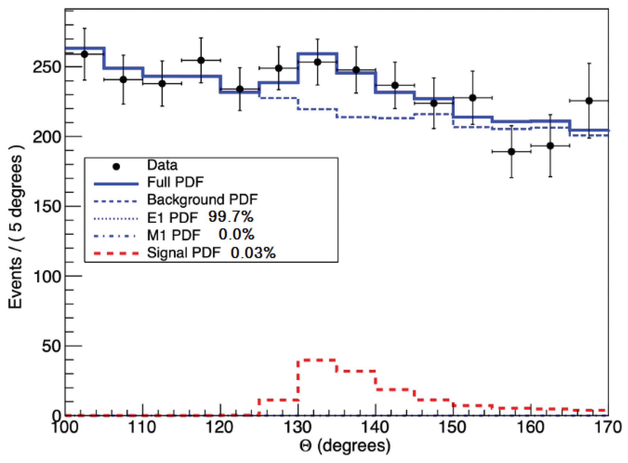
Finally, we changed the proton beam energy to 1225 keV, above to the 1040 keV resonance to check the off resonance region. The combined IPC simulation curve and experimental data for this transition is shown in Figure 11. It clearly shows a deviation in the

e^{+}

e^{-}

opening angle distribution between the data and the simulation around

135^{\circ}

. This deviation is in agreement with the result published by the ATOMKI collaboration in [1]. By assuming that the deviation is coming from the creation and immediate decay of an intermediate particle to an

e^{+}

e^{-}

pair, we can calculate a mass of

m_{X} c^{2} = 16.66 \pm 0.47

(stat.) MeV for this particle with a confidence above 4

σ

. As can be seen in the insert of Figure 11, we could describe the background with pure E1 distribution, which show that we are indeed in the off resonance region.

The systematic uncertainty on the calculated particle mass from the beam spot’s position was estimated using a series of simulations using different beam spot positions. This resulted in a

Δ m_{X} c^{2}

(systematic)=

\pm 0.35

MeV uncertainty.

Based on the best-fit results shown in Figure 11, it can be concluded that X17-boson particles were created simultaneously with the IPC due to the E1 transition in this experiment. The branching ratio of the

e^{+}

e^{-}

decay of such boson to IPC and

γ

decay of the 18.15 MeV level is found to be 2.8x

10^{- 3}

and 1.1x

10^{- 5}

, respectively. It seems that the X17 particle is created in the E1 transition and not in the M1 one. In Ref. [1], they obtained a branching ratio of 5.8x

10^{- 6}

, which is about half of the value we obtained here. They did the experiment on the 1040 keV resonance, in this way the M1 contribution of the resonance may not produced any X17 particle.

4. Summary

We successfully built a two-arm

e^{+}

e^{-}

spectrometer in Hanoi. The spectrometer was tested and calibrated using the 17.6 MeV M1 transition excited in the

{}^{7}{Li}

(p,

e^{+}

e^{-}

)

{}^{8}{Be}

reaction. We have got a nice agreement between the experimentally determined acceptance of the spectrometer with the one coming from our simulation. The angular correlation of the

e^{+}

e^{-}

pairs measured for the 17.6 MeV transition (E_p=441keV) agrees well with the simulated one for the M1 transition, and no anomaly was observed for this. However, a significant anomaly (

> 4 σ

) was observed for E_p=1225 keV, which is the off resonance region above the E_p=1040 keV resonance, at around

135^{\circ}

, in agreement with the ATOMKI results published in 2016[1]. The mass of the hypothetical particle from this result was obtained to be

16.66 \pm 0.47

(statistical)

\pm 0.35

(systematic) MeV. In the future, we are planning to upgrade the spectrometer to get a wider angular acceptance.

Author Contributions

Methodology, A.J.K.; software, A.K., D.T.K.L; formal analysis, T.T.A, T.D.T.; writing—original draft preparation, T.T.A., T.D.T., A.J,K.; performed experiment, all. All authors have read and agreed to the published version of the manuscript.

Funding

Not applicable.

Institutional Review Board Statement

Not applicable.

Informed Consent Statement

Not applicable.

Data Availability Statement

Not applicable.

Acknowledgments

T.D.T appreciates the support of the Institute of Physics, Vietnam Academy of Science and Technology.

Conflicts of Interest

The authors declare no conflicts of interest.

References

A.J. Krasznahorkay, M. Csatlós, L. Csige, Z. Gácsi, J. Gulyás, M. Hunyadi, I. Kuti, B. M. Nyakó, L. Stuhl, J. Timár, et al., Phys. Rev. Lett. 116 (2016) 042501.
J. Gulyás et al., Nucl. Instr. and Meth. in Phys. Res. A 808, 21 (2016).
M. E. Rose, Physical Review 76, (1949) 678–681. (2016).
Xilin Zhang, and Gerald A. Miller, Phys. Lett. B 813 (2021) 136061.
A.J. Krasznahorkay, M. Csatlós, L. Csige, J. Gulyás, A. Krasznahorkay, B. M. Nyakó, I. Rajta, J. Timár, I. Vajda, and N. J. Sas, Phys. Rev. C 104, 044003 (2021).
A.J. Krasznahorkay, A. Krasznahorkay, M. Begala, M. Csatlós , L. Csige, J. Gulyás, A. Krakó, J. Timár, I. Rajta, I. Vajda, N.J. Sas, Phys. Rev. C 106, L061601 (2022).
A.J. Krasznahorkay, et. al., J. Phys.: Conf. Ser. 1056 012028 (2018).
Daniele S. M. Alves, et. al. Shedding light on X17: community report. Eur. Phys. J. C 83, 230 (2023).
A. Kanakis-Pegios, V. Petousis, M. Veselský, Jozef Leja, and Ch. C. Moustakidis Phys. Rev. D 109, 043028 (2024).
The NA62 Collaboration, Physics Letters B 846 (2023) 138193.
Matheus Hostert and Maxim Pospelov, Phys. Rev. D 108, 055011 (2023).
Nguyen The Nghia, Vu Thanh Mai, Bui Van Loat, VNU Journal of Science Mathematics-Physics 27 (2011) 180.
Cuong Phan Viet et al., EPJ Web of Conferences 206 (2019) 08004.
J.Allison, et. al., Nuclear Instruments and Methods in Physics Research A 835, 186–225 (2016).
https://gitlab.com/atomki-nuclear-phys/cda ; http:/atomki-nuclear-phys.gitlab.io/cda.
D. R. Tilley, J. H. Kelley, J. L. Godwin, D. J. Millener, J. E. Purcell, C. G. Sheu, and H. R. Weller, Nucl. Phys. A 745, 155 (2004).
D. Zahnow, C. Angulo, C. Rolfs, S. Schmidt, W.H. SchultC, E. Somorjai, Z. Phys. A 351,229-236 (1995).
N.J. Sas,1 A.J. Krasznahorkay, et al., arXiv:2205.07744v1 (2022).

Figure 1. Schematic diagram of the

e^{+}

e^{-}

spectrometer focuses on 140 degree region.

Figure 1. Schematic diagram of the

e^{+}

e^{-}

spectrometer focuses on 140 degree region.

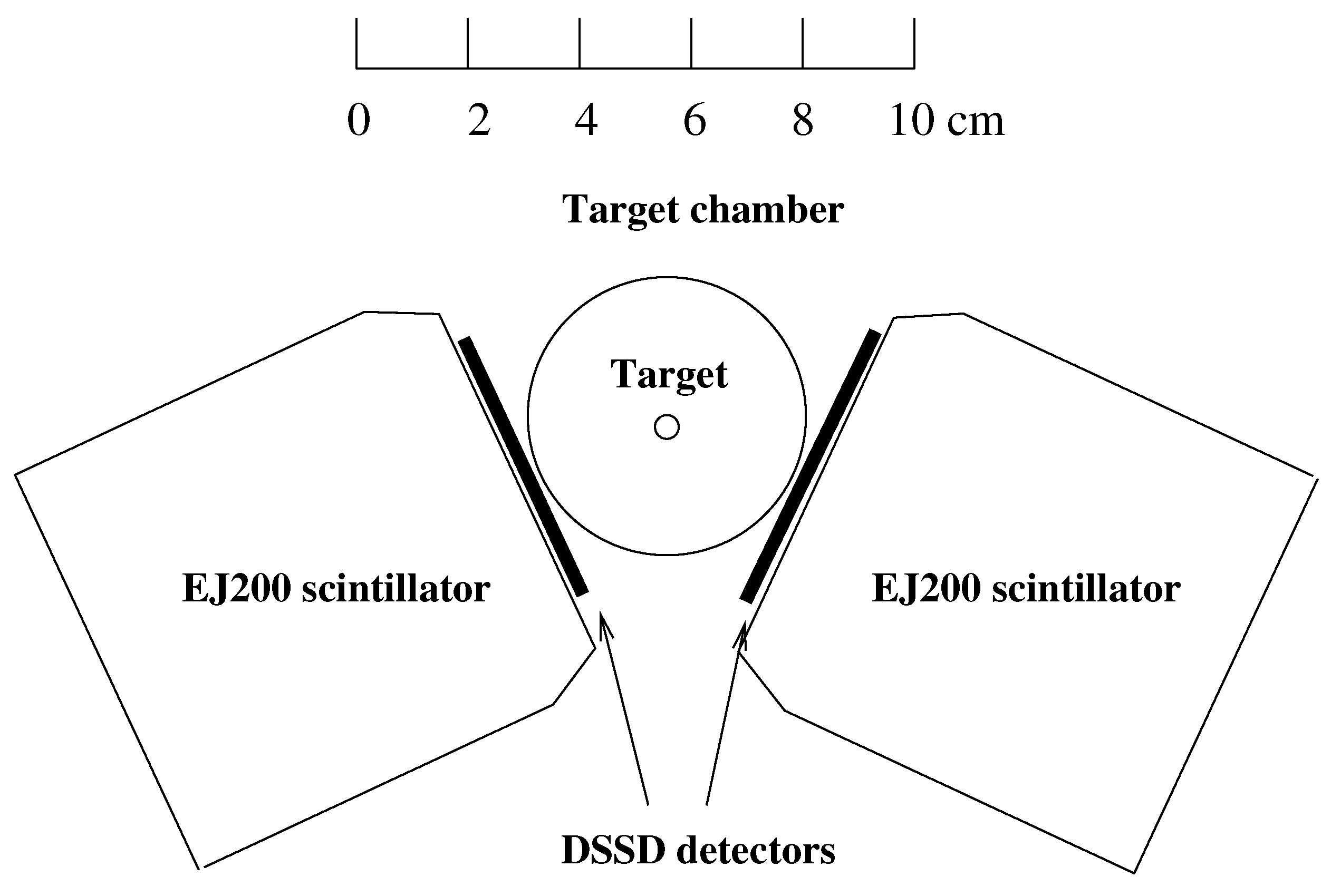
Figure 2. Time difference distribution between the two plastic scintillators using two cascade-gamma rays emitted from

{}^{60}{Co}

source.

Figure 2. Time difference distribution between the two plastic scintillators using two cascade-gamma rays emitted from

{}^{60}{Co}

source.

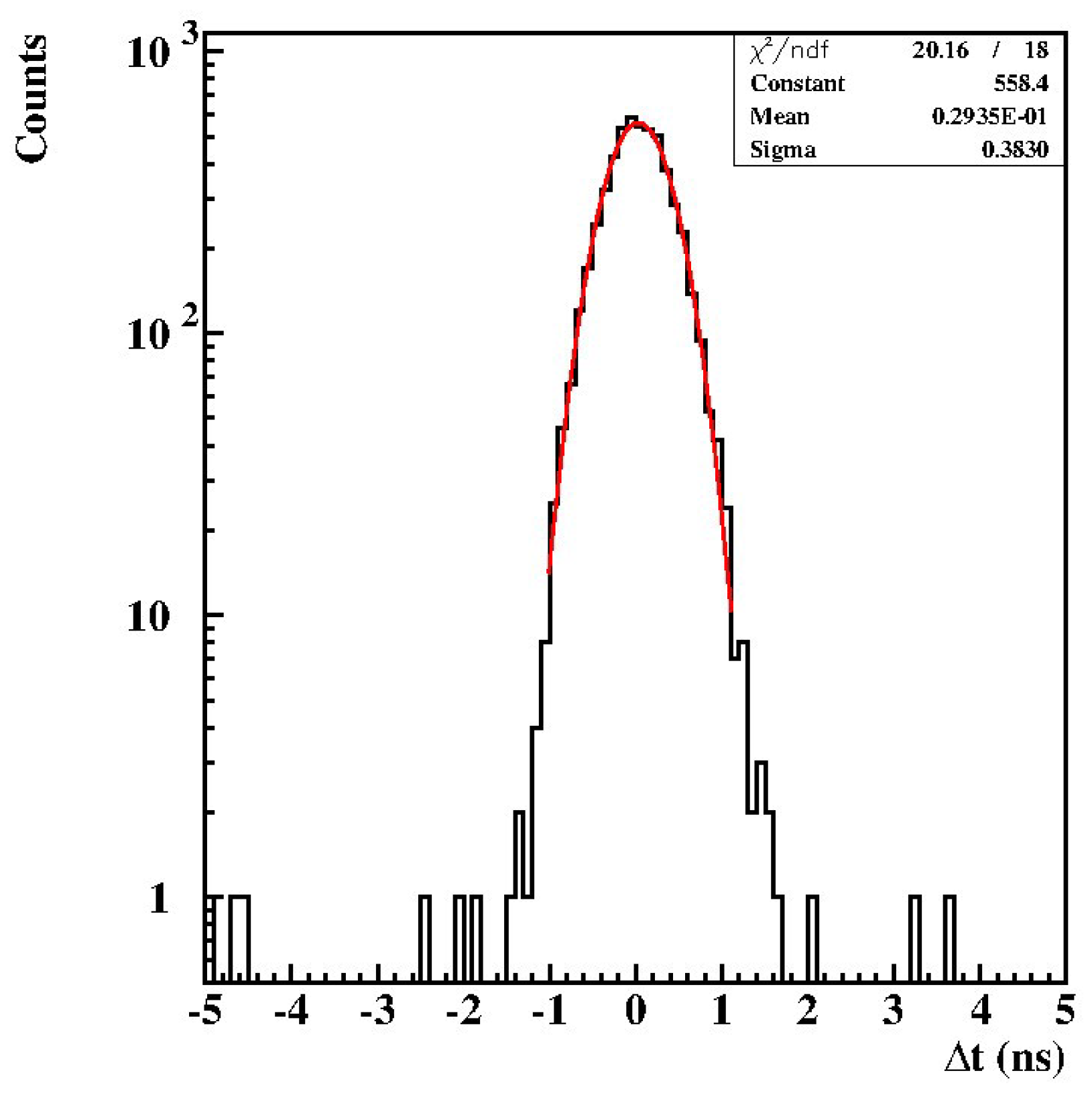
Figure 3. Electronic block diagram of the

e^{+}

e^{-}

spectrometer.

Figure 3. Electronic block diagram of the

e^{+}

e^{-}

spectrometer.

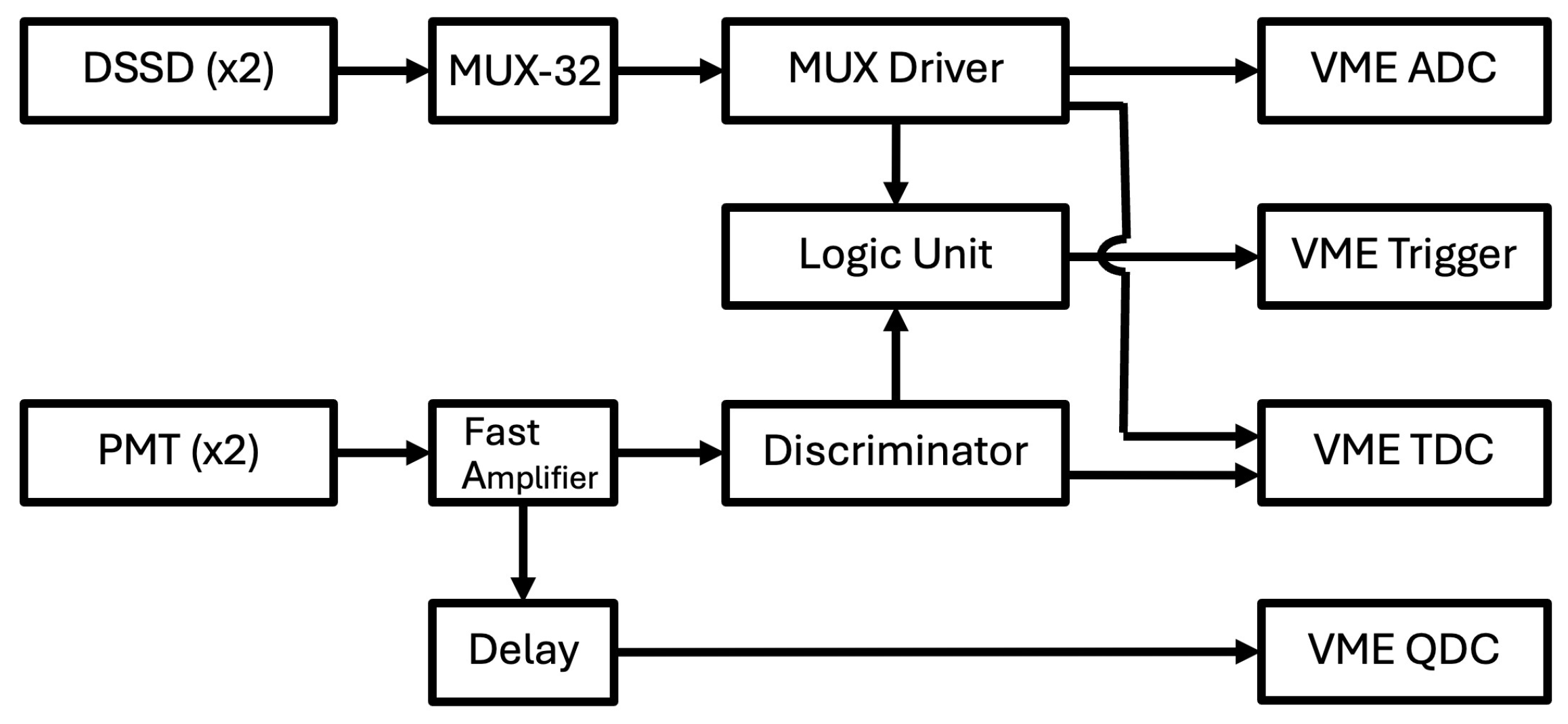
Figure 4. Typical measured (black histogram) and simulated (dashed line histogram) energy loss distributions of electrons and positrons passing through one of the DSSD detectors.

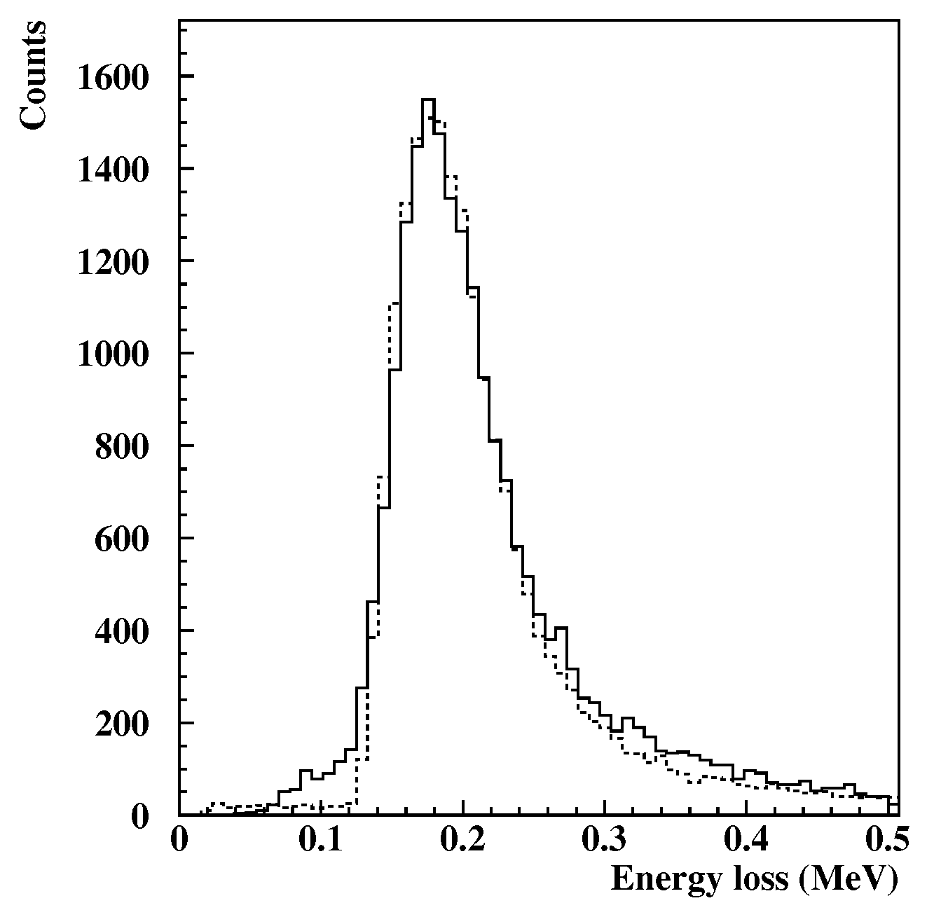
Figure 5. Left side: the x and y distribution of the position signals obtained from one of the DSSD detectors. Right side: 2D distribution of the position signals.

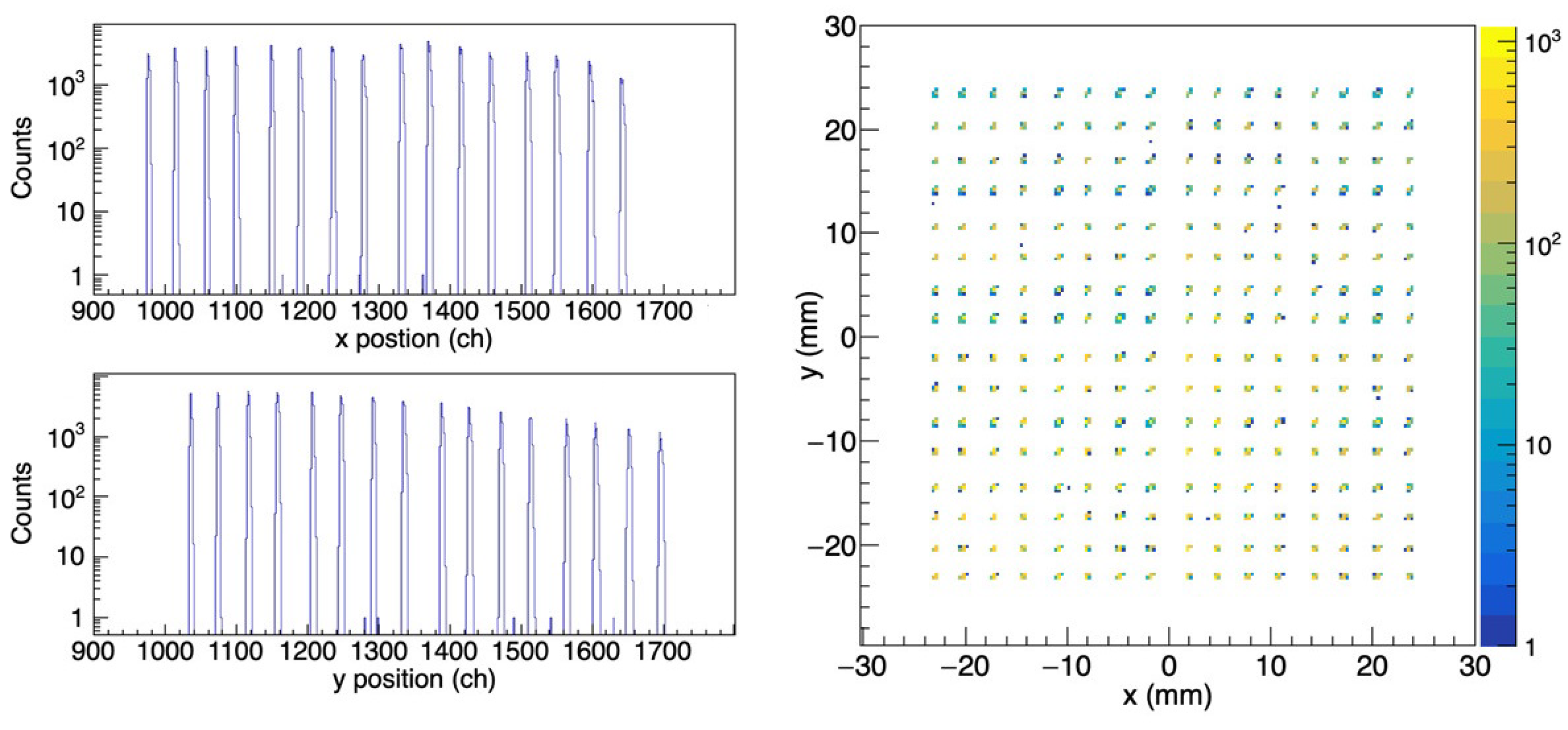
Figure 6. The total energy is deposited in a plastic scintillation of the

e^{+} e^{-}

pairs, which are selected by double-hit events in the corresponding DSSD. The peaks are from the transition indicated in the figure; the red line is a fitting line of a Gaussian with its center and sigma shown in the legend.

Figure 6. The total energy is deposited in a plastic scintillation of the

e^{+} e^{-}

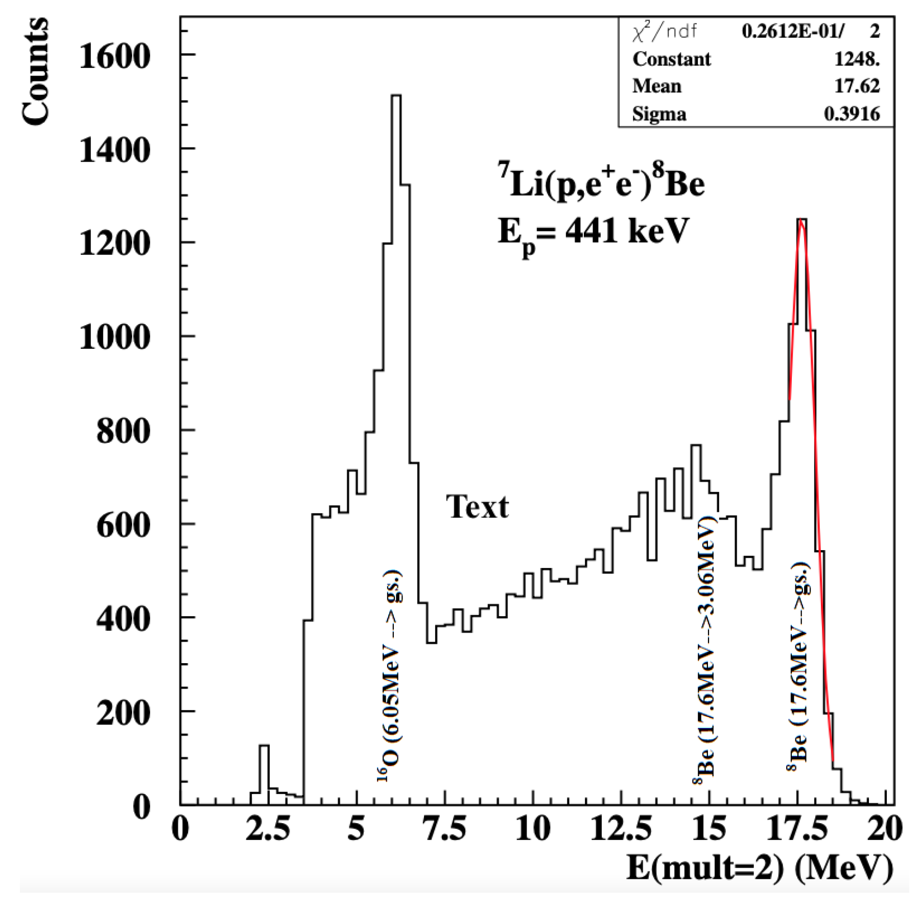
Figure 7. The excitation function of

{}^{8}{Be}

was obtained by scanning proton energy; the resonances of 17.6 and 18.15 MeV were seen as proton beams around 500 and 1040 keV, respectively. The measured data are shown by black dots with error bars and the dotted line connected the points is just drawn to guide the eye.

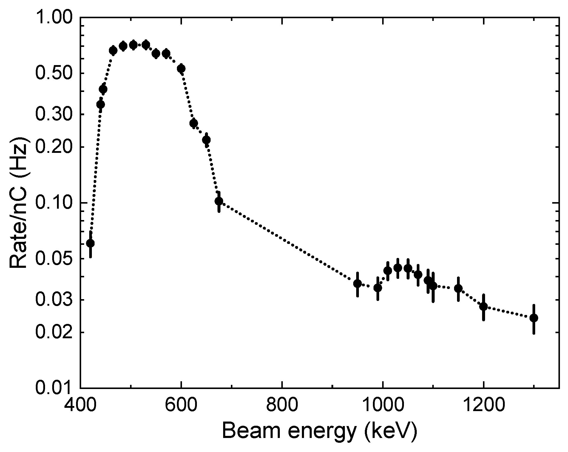
Figure 7. The excitation function of

{}^{8}{Be}

Figure 8. The acceptance curve of two-arm telescope system (left) and angular correlation of

e^{+}

e^{-}

pairs obtained from the 17.6 MeV transition using LiF target (right).

Figure 8. The acceptance curve of two-arm telescope system (left) and angular correlation of

e^{+}

e^{-}

pairs obtained from the 17.6 MeV transition using LiF target (right).

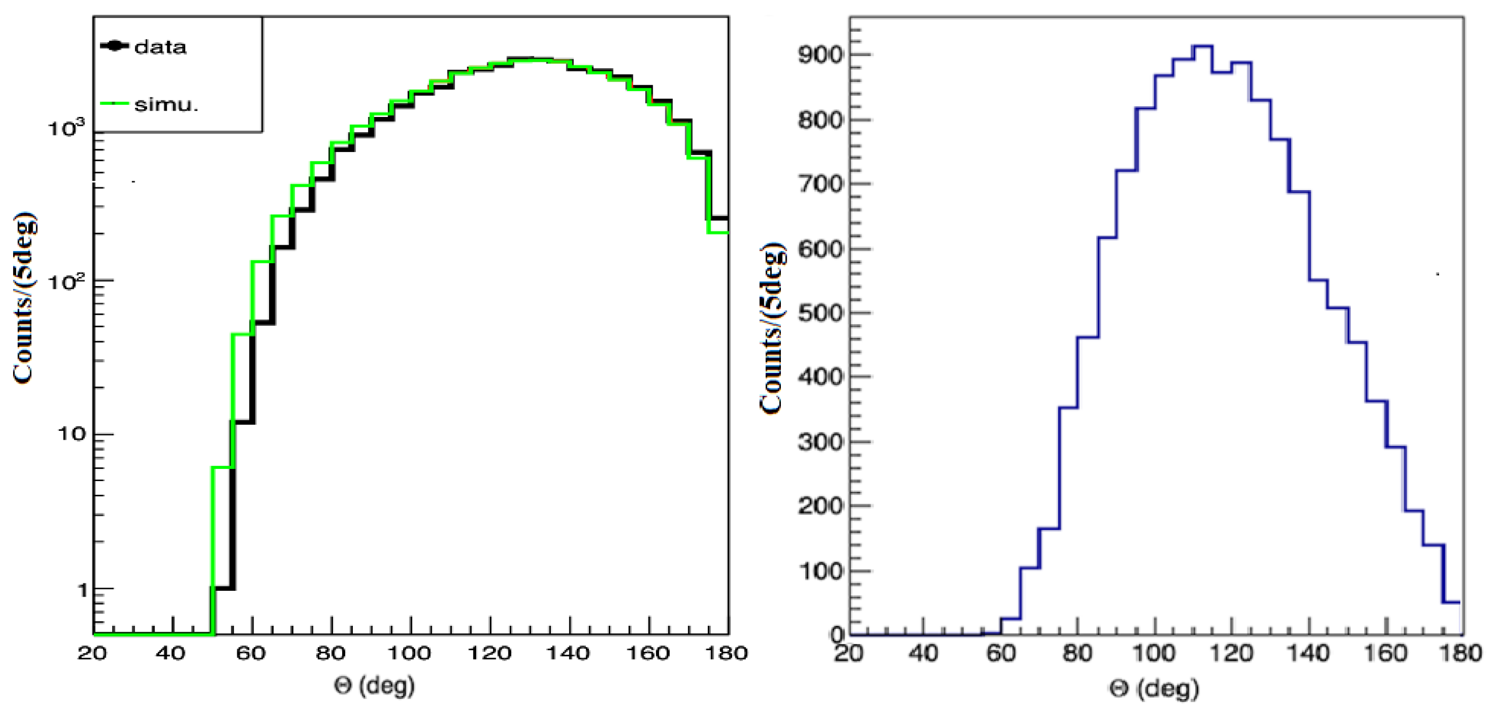
Figure 9. Angular correlation of

e^{+}

e^{-}

pairs when bombard LiF target by proton beam at 441 keV. The background line is the summing up of E1 and M1 lines, the numbers in the legend related to contribution of each terms, both the experimental data and simulations are corrected by the detection efficiency.

Figure 9. Angular correlation of

e^{+}

e^{-}

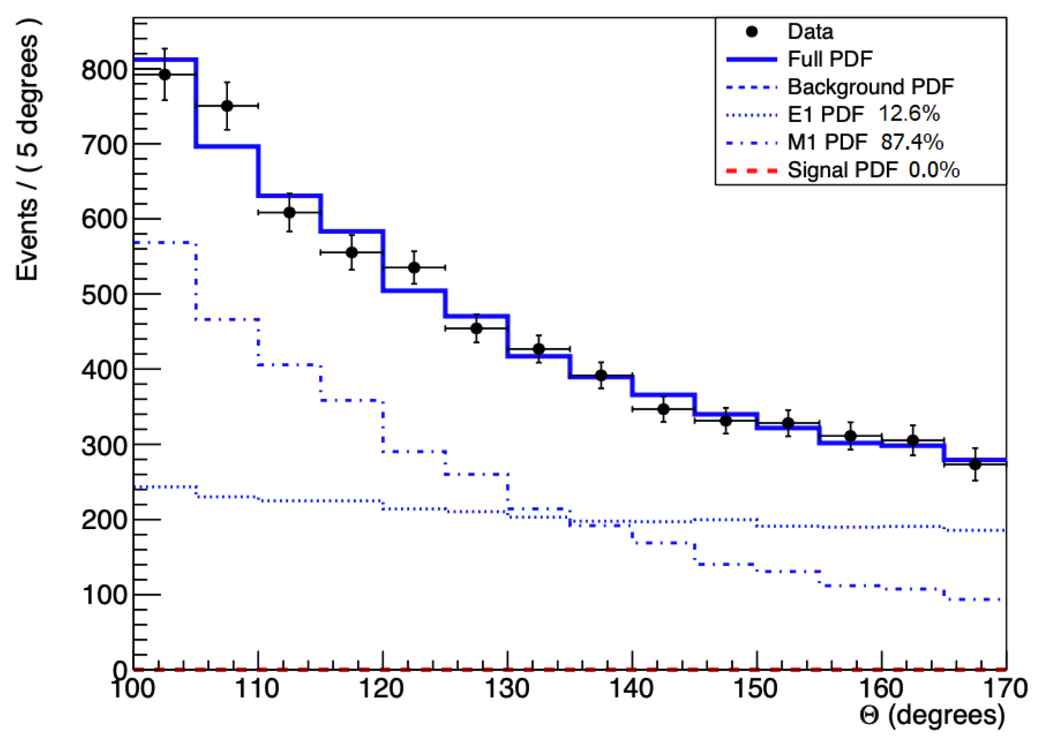
Figure 10. Similar to Figure 9 with 800 keV proton beam.

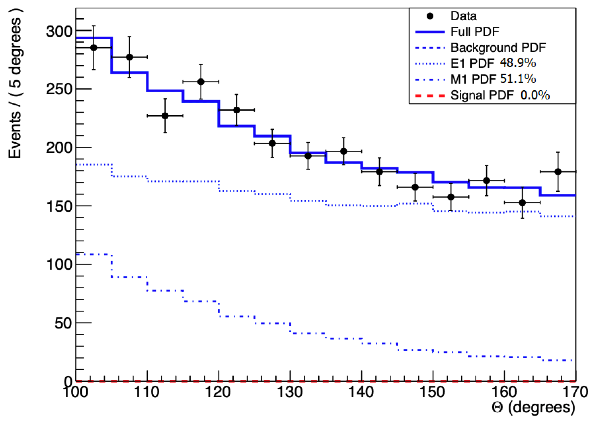
Figure 11. Angular correlation of

e^{+}

e^{-}

pairs when bombard Li₂O target by proton beam at E_p= 1225 keV. The background line is the summing up of E1 and M1 lines, the contribution of M1 transition is negligible, so the background line is overlap with E1 line.

Figure 11. Angular correlation of

e^{+}

e^{-}

Disclaimer/Publisher’s Note: The statements, opinions and data contained in all publications are solely those of the individual author(s) and contributor(s) and not of MDPI and/or the editor(s). MDPI and/or the editor(s) disclaim responsibility for any injury to people or property resulting from any ideas, methods, instructions or products referred to in the content.

© 2024 by the authors. Licensee MDPI, Basel, Switzerland. This article is an open access article distributed under the terms and conditions of the Creative Commons Attribution (CC BY) license (http://creativecommons.org/licenses/by/4.0/).

Copyright: This open access article is published under a Creative Commons CC BY 4.0 license, which permit the free download, distribution, and reuse, provided that the author and preprint are cited in any reuse.

MDPI Initiatives

Important Links

Choose an area of interest and we will send you notifications of new preprints at your preferred frequency.

Disclaimer

Checking the 8Be Anomaly with a Two-Arm Electron Positron Pair Spectrometer

Abstract

1. Introduction

2. Experimental Methods

2.1. The e + e − Spectrometer

2.2. Data acquisition system

2.3. Calibration of the DSSD Detectors

2.4. Calibration of the Scintillation Detectors

3. Experimental Results

4. Summary

Author Contributions

Funding

Institutional Review Board Statement

Informed Consent Statement

Data Availability Statement

Acknowledgments

Conflicts of Interest

References

MDPI Initiatives

Important Links

Subscribe

Checking the ⁸Be Anomaly with a Two-Arm Electron Positron Pair Spectrometer

2.1. The $e^{+}$ $e^{-}$ Spectrometer