Submitted:
04 March 2024
Posted:
04 March 2024
You are already at the latest version
Abstract
Statistical denoising techniques have been well studied, however many challenges still remain. This 9 article focuses on determining the least necessary number of significant samples in a statistical pop-10 ulation sampling, while minimizing the impact on the statistical detection of the fiber Bragg grating 11 (FBG) power spectra. This is achieved by using Bayesian decision making, small population statis-12 tics while excluding false detection. First, we investigate the impact of two-sided sliding window 13 technique applied near the cell under the test. The window size varies from 8 to 60 samples. The 14 considered maximum size of population sampling is connected with the number of wavelength 15 samples within the bandwidth of the symmetrical FBG power spectra peaks. Regarding the sym-16 metry of FBG power spectra peaks and the possible reduction of computational demands, we inves-17 tigate the impact of a one-sided sliding window. This enables to achieve less processing latency for 18 real time applications thus brings benefits to FBG-based fiber optical sensing. Both, two- and one-19 sided small population sampling techniques are then experimentally verified. Detection results are 20 analyzed in depth via calculating detection thresholds by using the small size window sliding along-21 side the waveband. From results achieved, it was found that the normality three-sigma rule does 22 not need to be followed while using the small population sampling. Experimental demonstrations 23 and analyses showed that the proposed concept of denoising and statistical threshold detection 24 based on the sliding window does not depend on the prior knowledge of probability distribution 25 functions of the FBG power spectra peaks level and background noise. We have also found that the 26 thresholds’ adaptability mainly depends on the statistical numerical characteristics of the above ad-27 ditive mixture of the FBG power spectra peaks signals and background noise.
Keywords:
statistically small population sampling
; two-sided sampling
; one-sided sampling
; 29 threshold detection
; fiber Bragg gratings
; FBG sensing
; optical spectrum analysis
1. Introduction
Measuring the resonant wavelengths of fiber Bragg grating (FBG) sensors, finding their fingerprints or classifying FBGs itself in optical sensing systems require denoising the acquired FBG spectral peaks [1,2,3,4,5,6,7] Meanwhile, all important properties of FBG spectral peaks have to be preserved.
To mitigate the impact of the background noise on the quality of the optical signals in the telecommunications and sensing systems, hardware pre-processing using real-time wavelength filtering has been typically used [8,9,10]. Software approaches based on verification or post-detection algorithms can be leveraged to detect signals in a complex or fluctuating background noise environment [11,12]. In the latter case, a variety of statistical detection techniques are usually applied. Such methods uzilize a preset level of an allowable detection threshold τ, relying on the signal-to-noise ratio (SNR) evaluation [12,13].
Previously [14,15], we reported on a denoising technique based on digital sliding window. In this case, the statistical detector has been introduced to detect spectral power of FBGs in an additive mixture of the signal and background noise. The statistical detector controls the power level depending on the given threshold level τ, as shown in Figure 1, indicating that the power level above the threshold belongs to FBG signal.
The decision function is based on the Bayesian decision theory [16,17,18] and Neyman-Pearson criteria [19] in order to minimize the false alarm probability pFA. The related decision-making process is shown in Figure 2.
In a previous study [15], a fixed K-number of the discrete power spectral samples were processed using the sliding window technique where K-number corresponded to a number of discrete wavelength steps within the FBG bandwidth. As was shown, K can be smaller. This depends on the requirement to either increase the threshold stability or to reduce the computational complexity. Statistical tests of reliability and validity showed the limits on the smallest K in the population sampling [16,17,18,19,20].
In this article, we focus on determining the least necessary but sufficient number of significant samples in statistically small population sampling while minimizing the impact on statistical numerical characteristics.
- First, we investigate the impact of two-sided sliding window sampling around the cell under the test;
- Second, we investigate the impact of one-sided sliding window.
In both these methods, K discrete steps related to the bandwidth of FBGs are applied.
Next, K will be gradually reduced to the smallest population sampling. This population sampling reduction will be done with respect to minimize the impact on statistical detection of the FBG power spectra.
In experimental demonstrations we will investigate how reducing K in the sliding window will impact the SNR and detection.
2. Statistical Thresholding Using Two-Sided Small Population Sampling
In this section, we study and analyze the symmetrical K-size two-sided population sampling, comprised of left and right sub-windows, see Figure 3.
Figure 3 illustrates the main principle of a statistical detection based on sliding window. As we have already explained, the comparator in the statistical detector decides whether the power level in the cell under the test (CUT) is above the threshold level τ. After the presence of FBG power spectra peaks was evaluated, the window is shifted by one wavelength step, and the adjacent cell becomes the CUT. This is why the window is called sliding window along the waveband. The waveband comprises of N number of cells each containing different power levels of the signal with noise.
Based on the Bayesian decision theory and Neyman-Pearson criteria, as well as with the minimum required false detection, pFA, the statistical detector is not allowed to exceed the preset value of pFA. In other words, at pFA = 10–3 maximum 1 false threshold detection is allowed from 1000 CUTs investigated.
2.1. Statistical Threshold Calculation
The calculation of the statistical threshold τ uses statistical characteristics of the additive mixture of the signal and background noise. This comprises the mean μK and the standard deviation σK. Both characteristics are calculated from the fixed number of K cells from the left and the right sub-windows. This can be called K-sized population sampling around the CUT. By default, a symmetric K-size window is chosen due to the typical symmetric Gaussian shape of the reflected FBG power spectra peaks [8,9,10,11]. The size of K depends on properties of FBGs, including the FBG bandwidth BFBG, sensing interrogator resolution δsens, and the effects of attenuation. In the following example, let assume BFBG = 0.8 nm and δsens = 0.008 nm. Thus, the above-threshold power can be approximated from M discrete wavelength steps as M ≅ BFBG / δsens = 100. As a rule, it is recommended to keep K ≅ M.
First, the calculated threshold τ has to contain the noise function fSMF describing attenuation approximation of the single-mode fiber (SMF-28). Second, an instrumental error function εinstr should be included. The εinstr is a sum of all instrumentation errors, and includes fluctuations in the wavelength discretization, quantization, deviations or offsets due to internal or external environmental changes. Generally, both functions are long-term stabilized, assuming stable operating conditions of the optical fiber and the FBG sensing interrogator.
Next, the calculation of τ has to include the required pFA (for example, pFA = ×10–3 … ×10–6). The smaller the pFA, the higher values of τ can be achieved. However, the threshold values should range from the minimum value slightly above the background noise energy Emin up to the maximum expected value of the additive mixture Emax (the FBG power spectra peak value with a background noise). Due to the above, the pFA is parameterized in the range from Emin to Emax. For large sampling populations, a full parametrization is required typically, and is equal to 1. However, for decreasing K-size, the pFA is parameterized with lower weights. The condition K < M allows for the adequate weakening of the pFA parametrization.
Finally, the calculated threshold τ has to include the additive mixture (N0 + ES)k obtained in the given kth CUT. This value should be weighted by both the mean μK and the standard deviation σK. Both are obtained from the K-size population sampling within the sliding window. If the K-size is reduced, the accuracy deteriorates and the parametrization of the (N0 + ES)k value is weakened accordingly. On the contrary, the increased standard deviation increases the contribution of the additive mixture in the calculation of τ.
To conclude, the parameterized pFA and (N0 + ES)k, will affect the fast dynamic adaptation of the threshold τ. The calculation of the threshold τ is given by the Eq. 1:
where G is the number of guard cells in the neighborhood of the CUT that do not participate in the threshold calculation. In general, the more guard cells, the smaller the weight of the parameterized pFA.
2.2. Experimental Demonstration and Results
The non-linear attenuation of the used optical fiber (G.652. D SMF) and the creation of the approximate broadband fSMF attenuation function is described in [21]. In the experimental demonstration, various optical fiber lengths are considered, representing the range of attenuation between – 1 ... – 45 dB. Several FBG optical sensors with a bandwidth of BFBG ≅ 0.8 nm and maximum attenuation of – 20 dB at the resonant wavelength λFBG are connected to optical fiber.
The digitized additive mixture of the signal and background noise (in the spectral domain) are continuously processed in the predefined wavelength sliding window of different K sizes. This sliding window systematically shifts and μK, σK and τ are dynamically calculated (Eq. 1) for each of the CUTk, see Figure 3. The G neighboring guard cells are excluded from μK, σK and τ computing.
In next subsections 2.2.1 and 2.2.2, different threshold values τ will be determined and investigated for different values of pFA for a different FBG power spectra peaks and the presence of the background noise.
The interrogator processes discrete power values for each discrete wavelength in the presence of the quantization noise. To compare different effects of instrumental distortion, a commercial interrogator and a table-top analyzer with a different wavelength resolution are used in experimental investigations.
2.2.1. Experimental Investigation of Two-Sided Small Population Sampling Using Interrogator
The commercial interrogator Sylex S-line S-400 [22] was used in this study, having the wavelength resolution of δsens = 0.08 nm. Because of slightly changing BFBG under the influence of fluctuating noise, the sampling with M = 9 ... 13 discrete values and BFBG ≅ 0.8 nm was selected. Four FBG sensors (A, B, C and D) were deployed within the C-band. The experimental results for various detection thresholds are shown in Figure 4. In addition, interfering spectra with ten times narrower FBG bandwidths (I to X) were implemented to demonstrate the advantage of dynamic thresholds adaptation. The variety of detection conditions due to partial overlap of FBG power spectra, their varying density distribution were investigated. Results are shown in Figure 4.
Due to a rapidly rising or descending σK at FBG power spectra peaks edges, the dynamic threshold “shakes”, especially when K = 8. In this case, the method is not appropriate for denoising threshold detection. However, the results for K = 10 or K = 12 indicate already adapted threshold τ to the additive mixture of signals and fluctuated background noise (see Eq. 1). Despite “shaky” thresholds can be also seen here, they are ~ 0.5 to 1.5 dB respectively above the background noise, and therefore the statistical detection of FBG power spectra peaks levels become more reliable. A further increase in K over M result in “shakeless” and increased τ values, thus yielding a safer detection of FBG power spectra. Therefore, the recommended setting is K ≅ M.
2.2.2. Experimental Investigation of Two-Sided Small Population Sampling Using Table-Top Analyzer
The analyzer AQ6370C [23] is used to process the transmitted power spectra with oversampled wavelength resolution of δsens = 0.0035 nm. Here, the sampling is done with discrete values of M = 90 ... 120 and BFBG ≅ 0.8 nm. Within the C-band, four FBG sensors (A, B, C and D) in the C-band are used. The results of various detection thresholds scenarios are shown in Figure 5. Here, the attenuation of the optical fiber was assumed – 35 dB with the highly fluctuated background noise (σK N0 ≅ 4.3 dB) and input power with of SNRin ≅ 8.5 dB. Despite of these unfavorable conditions, detectability and adaptability of τ are improved, compared to the previous case study.
As in the previous case study described in section 2.2.1, thresholds τ are also “shaky” for the same reasons. However, for M = 90 ... 120 and K = 8 ... 60, results obtained are significantly better despite those unfavorable detection conditions. Surprisingly, even for K = 12 or K = 16, the threshold detection results are acceptable and are comparable to the previous results in section 2.2.1 for K ≅ M.
In Figure 5 can be noted a sudden / significant drop in the threshold values τ in the close proximity of the FBG power spectra peaks. The deeper the drop of threshold values (especially when K is much less than M), the higher is the difference which is helping to improve the SNR. This value differences are illustrated in Figure 6.
In Figure 6 (a), pFA ≈ 10—3 and K = 10, a random low level false detection occurred for power levels below 1.2 dB. This effect was well suppressed for K = 12 and the detected FBG power level spectra doubled approaching 7 dB. When K = 16 … 32, FBG power spectra peaks levels are reliable detected without false detection.
When pFA ≈ 10—4 (case Figure 6 (b)), all thresholds rise to their higher level. As a consequence, no false detections was observed for K = 12 and. Only a few false detections occurred for K = 10. Similarly, K = 16 … 32 allowed to maintain reliable detection of the FBG power spectra peaks levels without false detections. However, the highest level of K = 60 (the strictest threshold) causes the FBG detection loss.
2.3. Threshold Behavior Analysis and Discussion
In this subsection, a mathematical analysis of the threshold calculation is presented and implications for the detection of the FBG power spectra peaks are derived.
Let us first analyze the parameterization of the 3rd component of Eq 1. We assume a typical FBG power attenuation ranging in interval (Emax … Emin) = 20 dB and a typical maximum value of pFA ≤ 10– 3. As a result, the 3rd component in Eq. 1 ranges from – 1.45 to – 2.8 dB for the population sampling K = 4 ... 60, and assuming 1 guard cell adjacent to the CUT in each of sub-windows:
If K = 60, the 3rd component parametrization is equal to – 2.8 and will cause reduced threshold τ. On the contrary, for K = 4, the 3rd component parametrization is equal to –1.45 and will cause an increased τ, see Eq. 1. This property can be used to set the value of τ which will be used later.
Next the 4th component in Eq.1 will be analyzed in the presence of background noise only ((N0 + ES)k = N0k). Here, K value affects the threshold calculation through changes of statistical characteristics of μK and σK as follows:
Finally, the total contribution of the 4th component to the threshold calculation of Eq. 1 without the occurrence of FBG power spectra peak is:
From the above it can be shown that approximately 3-fold increase in contribution of the 4th component (from 0.002253 in case of K = 60 to 0.006747 in case of K = 30, respectively) can be achieved, thus contributing to the threshold level increases.
Let’s now analyze the μK-parameterization of (N0 + ES)k in Eq. 1 when the approximately Gaussian shaped FBG power spectra peak overlaps with the sliding window. Using the example from section 2.2.1, and using K = M/2 ≅ 60, the mean values keep increasing from the lowest to the highest values just in 30 wavelength steps. At the 60th step, where CUTk contains the FBG power spectra peak maxima, the two-sided sampling reaches the value μK=60 ≅ 2 ∙ 0.25 ∙ (Emax … Emin) above the N0 noise level. When the sliding window touches the falling edge of the FBG power spectra peak and starts to leave it, the mean value μK starts decreasing. However, for M/2 ≅ 60 and K = 30, the behavior of the mean values will remain mostly unchanged. To be noted, for the 60th step the shorter the sliding window, the higher mean value μK. When K=10, μK=10 ≅ 0.707 ∙ (Emax … Emin).
Now we analyze the σK-parameterization of (N0 + ES)k in Eq. 1 when the approximately Gaussian shaped FBG power spectra peak overlaps with the sliding window. This is shown in Figure 7 (b). For K = M/2 ≅ 60, the standard deviation values achieve the highest values in ~ 30th and ~ 90th step. Here, the square root multiplier in Eq. 4 achieves the widest span of input values. It is worth noting that the σK-parametrization on the leading and falling edges can reach similar effects as the μK-parametrization. This depends on the steepness of edges. When the sampling window slides from 30th to 90th step, the σK value drops. For M ≅ 60 and K = 30, the behavior of the standard deviation values will be similar to the case of K = M/2 ≅ 60. To be noted, the longer the sliding window, the larger is the standard deviation σK. This is the origin of threshold adaptability.
Finally, a comparison of the magnitudes μK and σK in Figure 7 points out the impossibility of meeting the empirical three-sigma rule (known also as the 68-95-99.7 rule) which is used to verify the normality of population sampling. In spite of this, the use of two-sided small population sampling is reliable for successful statistical threshold detection. This was illustrated by results in Figure 4, Figure 5 and Figure 6.
3. Statistical Thresholding Using One-Sided Small Population Sampling
In this section, we study and analyze the impact of the population sampling using one (left) sided window having an asymmetrical K/2-size, see Figure 8.
3.1. Statistical Threshold Calculation
The calculation of the statistical threshold τ uses the mean μK/2 values and the standard deviation σK/2 values obtained from the fixed number of K/2-cells contained in the left sub-window. Please note that the sliding window is asymmetrically located, in this case sitting on the left side, see Figure 8. This reduces the computation complexity by excluding the right-side sub-window from population sampling. In the next step, we will investigate the impact of this approach on the quality of the threshold detection results. Since the shape of the reflected FBG power spectra is typically symmetric Gaussian function, we need to learn if in this approach the μK/2, σK/2 and τ would differ from the two-sided μK and σK/2, respectively. Similar to section 2.1, calculation of the threshold τ will use the Eq. 1.
3.2. Experimental Demonstration and Results
To compare the effect of halving the population sampling, the same considerations, instrumentation and conditions are applied in the experimental investigation as in the previous section 2.2.
3.2.1. Experimental Investigation of One-Sided Small Population Sampling Using Interrogator
Here, as described in section 2.2.1, the same commercial interrogator and the same deployment scenario of four FBG sensors A, B, C and D along the C-band with M = 9 … 13, interfered by narrowband FBGs I … X, was used.
Results are shown in Figure 8 indicating various threshold detection. As the sliding window approaches individual FBG power spectra levels (Note: sliding window shifts from lower to higher wavelengths), the thresholds keep increasing very slowly. This is due to a weak mean values μK/2. Please compare results in Figure 4 and the discussed effect of μK in section 2.3. After passing through the FBG power spectra peaks, the thresholds behavior stabilizes. This is similar to behavior shown in Figure 4. However, the cells reduction from K to K/2 noticeably causes higher fluctuations of σK/2 thus calculated τ, especially when K/2 < M. Therefore, this scenario is not recommended for system operation. On other hand, thresholds τ for K/2 = 8 ... 16 ≅ M adapts very well to the signal / noise behavior. For further increases in K/2, when K/2 > M, threshold τ rises accordingly, which may lead to the power loss related to the right side of the FBG power spectra. In summary of the above, it is recommended to use K/2 ≅ M.
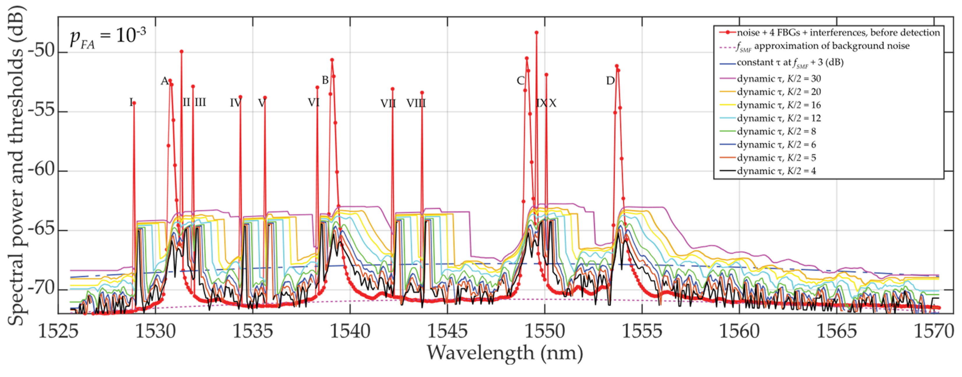
Figure 9.
Results of dynamic statistical threshold detection of the wideband (A, ... , D) and narrowband (I, ... , X) FBGs with different power levels, pFA ≈ 10—3 and K/2 = 4 ... 30.
Figure 9.
Results of dynamic statistical threshold detection of the wideband (A, ... , D) and narrowband (I, ... , X) FBGs with different power levels, pFA ≈ 10—3 and K/2 = 4 ... 30.
3.2.2. Experimental Investigation of One-Sided Small Population Sampling Using Table-Top Analyzer
The same table-top analyzer was used to process the transmitted power spectra of four deployed FBG sensors within the optical fiber C-band using values M = 90 … 120. The experimental results of various detection thresholds τ are shown in Figure 10.
It can be noted again that the thresholds “shake”, here slightly more than in the case illustrated in section 2.2.2. This is due to the smaller mean μK/2 values compared to μK values. As the sliding window approaches FBG power spectra peaks, the threshold values increase slowly and better adapt to FBG power spectra levels with background noise. After passing the FBG power spectra peak maxima, the behavior of the threshold levels stabilizes similarly to those in Figure 5. A greater “shaking” was observed for K/2 = 4 … 6 << M. This causes rising in false detection. For K/2 = 8 … 16 (smaller than M), the detection results are acceptable and comparable to the investigation in section 2.2.2 with K = 12 or K= 16 when K = M. The previously observed phenomenon of dropping τ values in the vicinity of FBG power spectra peaks appeared also here and again helps to improve the SNR, see Figure 11.
The detected power levels of the 4 FBGs by using one-sided sliding windows for K/2 = 4 … 30 is shown in Figure 11. In cases when K/2 = 4 … 6, thresholds are “very shaky” thus the threshold detection is not reliable leading to increased false detections. In contrast to Figure 6, all FBG power spectra are tilted and sharpened. This is an artefact caused by one-sided population sampling. When pFA ≈ 10—3 (see Figure 11 (a)), false detections are noted at levels below 1 dB when K/2 = 8. No false detections occur for K/2 > 8. In contrary to results shown in Figure 6, here the detected power levels of the FBG power spectra are slightly higher, thus the one-sided population sampling performs better than using two-sided population sampling in section 2.2.2.
When pFA ≈ 10—4 shown in Figure 11 (b), all threshold levels are increased. Therefore, no false detections are noted when K/2 = 8 … 30 with one exception when λFBG = 1549.1 nm. Here, the large fluctuation of the background noise resulted in the “shaky” threshold behavior. Similar to situation in Figure 11 (a), the K/2 = 12 … 30 values allow maintaining the FBG power spectra levels at the reliable detection level thus without false detections. However, in contrast to Figure 6, there is no loss in the FBG power spectra detection when K/2 = 60.
3.3. Threshold Behavior Analysis and Discussion
In this subsection, a brief analysis of the threshold calculation and behavior is given.
Let’s analyze the parameterization of the 3rd component of equation 1. Considering the same conditions as in section 2.3, but half K to K/2 = 2 … 30, equation 2 will be:
Solution of Eq. 2 and Eq. 6 in terms of K is value equal K/2 that is identical for both, one-sided and two-sided population sampling.
Let us now analyze the parameterization of the last component of Eq. 1 with the presence of the background noise only, (N0 + ES)k = N0k. Here, K/2 value affects the threshold calculation through changes of statistical characteristics of the μK/2 and σK/2:
Here, the numerical values of μK/2 found in Eq. 7 are half of μK values found in Eq. 3. Because the number of the selected values xi is also halved, then μK/2 ≅ μK in cases of uniform statistical distribution. The numerical values of σK/2 found from Eq. 7 differ from σK given by Eq. 4. In summary, due to computational demands, the selection of K/2 over K is preferable but is governed by the availability of a number of cells with required properties.
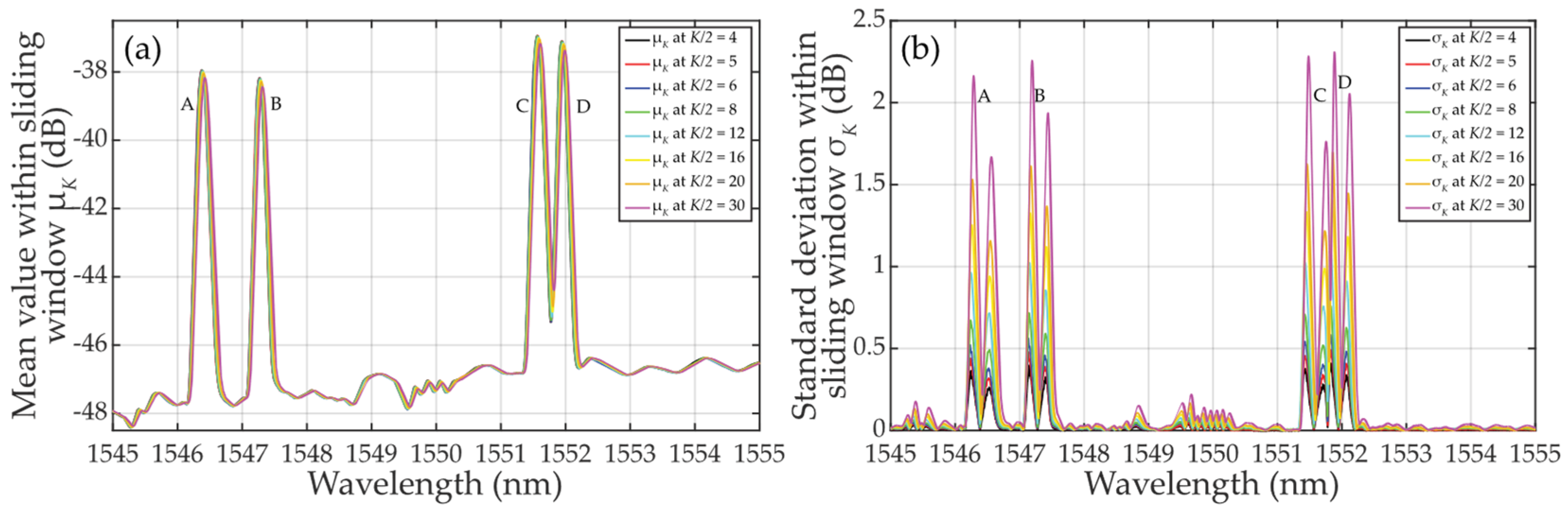
Based on Eq. 7, we have also analyzed the μK/2-parameterization of (N0 + ES)k in case of when the leading edge of FBG power spectra overlaps with the sliding window. This is shown in Figure 12 (a) in case of small population sampling when K/2 = 4 … 30. Increase of the mean μK/2 values is similar to the case of μK when K = 8 … 32 (see Figure 7 (a)). Overall, the behavior of the mean of μK/2 and μK values related to any FBG power spectra in the presence of noise is nearly identical, except when K = 32 ... 60 where μK is slightly lower, see Figure 7.
Based on Eq. 8, we then analyzed the σK/2-parameterization of (N0 + ES)k in case when the leading and falling edges of FBG power spectra are part of the sliding window. For K/2 << M or K/2 < M, the standard deviation exhibits two local maxima in the close proximity of the FBG power spectra peak, see Figure 12 (b). It can be seen that the σK/2 value drops in between the two σK/2 maxima. The smaller the population sampling, the deeper the drop of σK/2. When comparing σK/2 in Figure 12 (b) to σK in Figure 7 (b), due to smaller population sampling the σK/2 maxima values are smaller. The left one-sided population sampling causes the higher rise of the left σK/2 maxima compared the one on its right. This obscures the threshold detection levels. From the above and Figure 9 and Figure 10, it can be concluded that the thresholds on the left side of the FBG power spectra peaks are better adapted to the signal plus background noise levels. Therefore, the outcomes of the “K/2 approach” described in section 3 are superior to those “K approach” described in section 2.
4. Conclusions
In our recent [15] digital sliding window denoising technique, a number of discrete power spectral population samples were processed. In order to increase computational efficiency, it is possible in some cases to reduce population sampling while maintaining the success of statistical detection. In this article we focused on determining the small population sampling for sufficient detection of fiber Bragg gratings power spectra in optical fiber sensing system. For such statistical threshold detection, the highest allowed number of false detections is set, which is based on the Bayesian principle.
In this article, the two-sided and one-sided statistical detectors have been introduced with reduced population sampling. In addition to the explanation of the method and the introduction of the main algorithms, a mathematical assessment of the impact of statistical characteristics, mean and standard deviation, are presented for various population sampling reductions. Next, reduced population sampling is applied using two common instrumentations for fiber optic sensing: using a commercial interrogator with standard wavelength resolution and a laboratory analyzer with improved wavelength resolution. We thereby confirmed the success of the statistical threshold detection under various conditions of fluctuating background noise, signal-to-noise ratio, approaching the adjacent fiber Bragg grating power spectra, and interferences by other signals. As from the demonstrated examples, statistical characteristics impact on statistical threshold detection were deeply analyzed for different false detection requirements. As a result, reduced number (12 to 16) samples are recommended for the two-sided sliding window in both used instrumentations. Similarly, 8 to 16 samples are recommended for the one-sided sliding window.
Supplementary Materials
The following supporting information can be downloaded at the website of this paper posted on Preprints.org. All concepts, methodologies, validations and formal analyzes are presented in the article to the extent acceptable. Supplementary materials can be made available after meaningful agreement with the authors.
Author Contributions
Conceptualization, G.C.; methodology, G.C.; software, G.C.; validation, G.C., D.B. and J.D.; formal analysis, G.C.; investigation, G.C. and J. D.; resources, G.C.; data curation, G.C. and J. D.; writing—original draft preparation, G.C.; writing—review and editing, G.C., D. B. and I.G.; visualization, G.C. and J. D.; supervision, G.C.; project administration, G.C. and D.B.; funding acquisition, D.B. All authors have read and agreed to the published version of the manuscript.
Funding
This research was funded by Slovak Grant Agency (VEGA) under Grant 1/0113/22, and in part by Slovak Research and Development Agency under Grants APVV-21-0217 and APVV-17-0631.
Informed Consent Statement
Not applicable.
Data Availability Statement
Supplementary materials can be made available after meaningful agreement with the authors.
Conflicts of Interest
The authors declare no conflict of interest. The funders had no role in the design of the study; in the collection, analyses, or interpretation of data; in the writing of the manuscript; or in the decision to publish the results.
References
- Li, H.; Li, K.; Li, H.; Meng, F.; Lou, X.; Zhu, L. Recognition and classification of FBG reflection spectrum under non-uniform field based on support vector machine. Opt. Fiber Technol. 2020, 60 (art. no. 102371), p. 9. [CrossRef]
- Mustapha, S.; Kassir, A.; Hassoun, K.; Dawy, Z.; Abi-Rached, H. Estimation of crowd flow and load on pedestrian bridges using machine learning with sensor fusion. Automation in Construction 2020, 112 (art. no. 103092). [CrossRef]
- Lv, Z.; Wu, Y.; Zhuang, W.; Zhang, X.; Zhu, L. A multi-peak detection algorithm for FBG based on WPD-HT. Optical Fiber Technology 2022, 68 (art. no. 102805). [CrossRef]
- Yan, Q.; Che, X.; Li, S.; Wang, G.; Liu, X. π-FBG Fiber Optic Acoustic Emission Sensor for the Crack Detection of Wind Turbine Blades. Sensors 2023, (art. no. 7821). [CrossRef]
- Zhichao, L.; Xi, Z.; Taoping, S.; Jiahe, M. Heartbeat and respiration monitoring based on FBG sensor network. Optical Fiber Technology 2023, 81 (art. no. 103561). [CrossRef]
- Liu, Q.; Yu, Y.; Han, B.S.; Zhou, W. An Improved Spectral Subtraction Method for Eliminating Additive Noise in Condition Monitoring System Using Fiber Bragg Grating Sensors. Sensors 2024, 24 (art. no. 443). [CrossRef]
- Zhuang, Y.; Han, T.; Yang, Q.; O’Malley, R.; Kumar, A.; Gerald, R.E., II; Huang, J. A Fiber-Optic Sensor-Embedded and Machine Learning Assisted Smart Helmet for Multi-Variable Blunt Force Impact Sensing in Real Time. Biosensors 2022, 12 (1159). [CrossRef]
- Madsen, C. K.; Lenz, G. Optical all-pass filters for phase response design with applications for dispersion compensation. IEEE Phot. Technol. Lett. 1998, 10 (7), pp. 994–996. [CrossRef]
- Kumar, S.; Sengupta, S. Efficient detection of multiple FBG wavelength peaks using matched filtering technique. Opt. Quantum Electron. 2022, 54 (2, art. no. 89), p. 14. [CrossRef]
- Tosi, D. Review and analysis of peak tracking techniques for fiber Bragg grating sensors. Sensors 2017, 17 (10, art. no. 2368), p. 35. [CrossRef]
- Guo, Y.; Yu, C.; Ni, Y.; Wu, H. Accurate demodulation algorithm for multi-peak FBG sensor based on invariant moments retrieval. Opt. Fiber Technol. 2020, 54, p. 9. [CrossRef]
- Meshcheryakov, R.; Iskhakov, A.; Mamchenko, M.; Romanova, M.; Uvaysov, S.; Amirgaliyev, Y.; Gromaszek, K. A Probabilistic Approach to Estimating Allowed SNR Values for Automotive LiDARs in ‘Smart Cities’ under Various External Influences. Sensors 2022, 22 (2, art. no. 609), p. 31. [CrossRef]
- Chen, Y.; Liu, Z.; Liu, H. A method of fiber Bragg grating sensing signal de-noise based on compressive sensing. IEEE Access 2018, 6, pp. 28318–28327. [CrossRef]
- Cibira, G. Simplified Statistical Thresholding Techniques for Dynamic Bandwidth Allocation in Shared Super-PON. In Proceedings of 14th intl. conf. ELEKTRO, Krakow, Poland, (23-26 May 2022). [CrossRef]
- Cibira, G.; Glesk, I.; Dubovan, J. SNR-based Denoising Dynamic Statistical Threshold Detection of FBG Spectral Peaks. J. Light. Technol. 2023, 41 (8), pp. 2526–2539. [CrossRef]
- Spiegelhalter, D. J.; Best, N. G.; Carlin, B. P.; van der Linde, A. Bayesian measures of model complexity and fit. J. Roy. Statist. Soc. Ser. B 2002, 64 (4), pp. 583–639. [CrossRef]
- Johnson, N. L.; Kotz, S.; Balakrishnan N. Continuous Univariate Distributions, 2nd ed.; John Wiley & Sons: New York, NY, USA, 1994; Volume 1, 573-627.
- Jacod, J.; Protter, P. Probability Essentials. 2nd ed.; Springer-Verlag Berlin: Heidelberg, Germany, 2004.
- Griffith, T.; Baker, S.-A.; Lepora, N. F. The statistics of optimal decision making: Exploring the relationship between signal detection theory and sequential analysis. J. Math. Psychol. 2021, 103 (art. no. 102544), p. 17. [CrossRef]
- Jones, A.R. Probability, Statistics and Other Frightening Stuff. 1st ed.; Routledge - Taylor & Francis Group: New York, NY, USA, 2018; Volume II, pp. 1-439.
- ITU-T G.652: Characteristics of a single-mode optical fibre and cable. Available Online: Available: https://www.itu.int/rec/T-REC-G.652-201611-I/en (accessed 23 Feb 2024).
- Sensing systems. Available online: https://www.sylex.sk/products/sensing-systems/interrogators/.
- Optical spectrum analyzer. Available online: https://cdn.tmi.yokogawa.com/files/uploaded/BUAQ6370C_01EN.pdf.
Figure 1.
Principle of statistical detection of the FBG power spectra peaks in the additive mixture of the signal and background noise.
Figure 1.
Principle of statistical detection of the FBG power spectra peaks in the additive mixture of the signal and background noise.
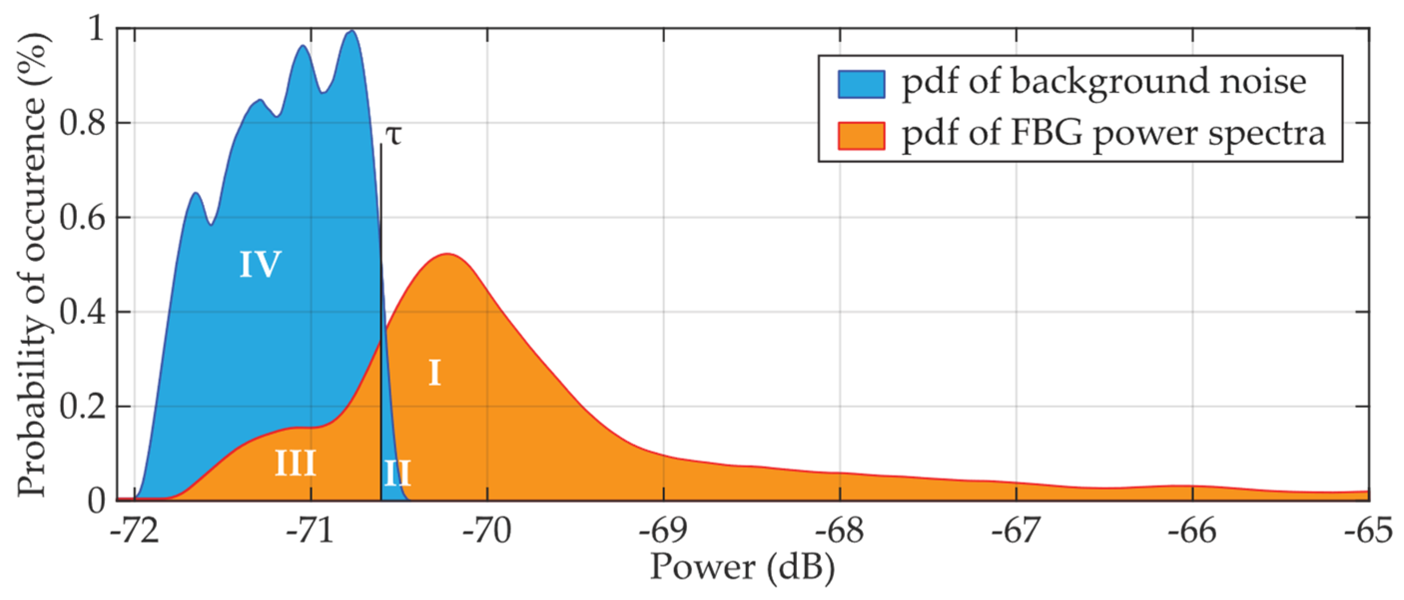
Figure 2.
Basic principle of the decision-making process.
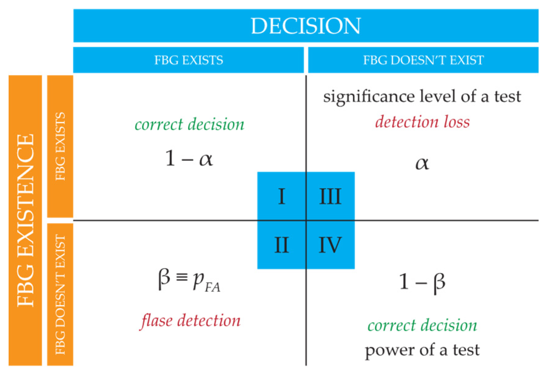
Figure 3.
Concept of the statistical threshold detector of FBG power spectra peaks level with a symmetric two-sided K-size sliding window.
Figure 3.
Concept of the statistical threshold detector of FBG power spectra peaks level with a symmetric two-sided K-size sliding window.

Figure 4.
Results of dynamic statistical threshold detection of the wideband (A, ... , D) and narrowband (I, ... , X) FBGs with different power levels, pFA ≈ 10—3 and K = 8 ... 60.
Figure 4.
Results of dynamic statistical threshold detection of the wideband (A, ... , D) and narrowband (I, ... , X) FBGs with different power levels, pFA ≈ 10—3 and K = 8 ... 60.
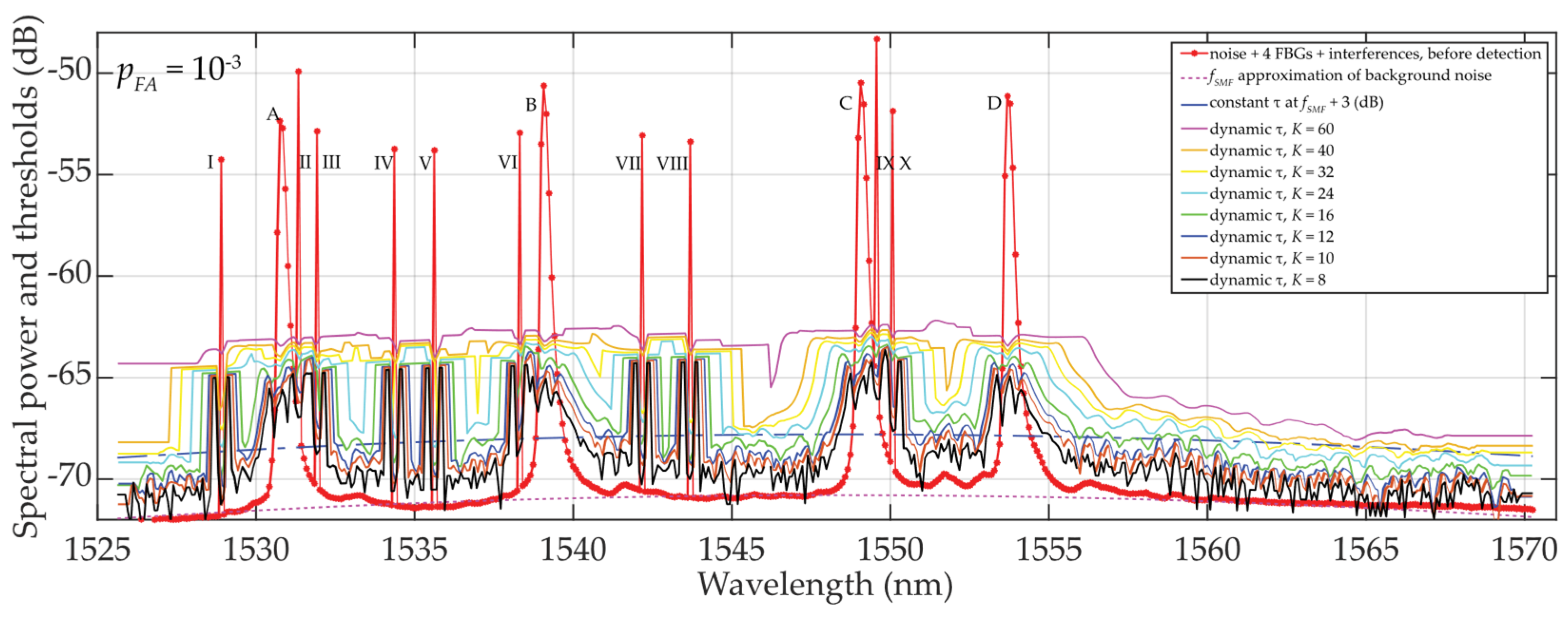
Figure 5.
Results of dynamic statistical threshold detection of the wideband (A, ... , D) FBGs with different power levels, pFA ≈ 10—3 and K = 8 ... 60.
Figure 5.
Results of dynamic statistical threshold detection of the wideband (A, ... , D) FBGs with different power levels, pFA ≈ 10—3 and K = 8 ... 60.

Figure 6.
Illustration of value differences of the wideband (A, ... , D) FBGs when K = 10 … 60: (a) pFA ≈ 10—3; (b) pFA ≈ 10—4.
Figure 6.
Illustration of value differences of the wideband (A, ... , D) FBGs when K = 10 … 60: (a) pFA ≈ 10—3; (b) pFA ≈ 10—4.
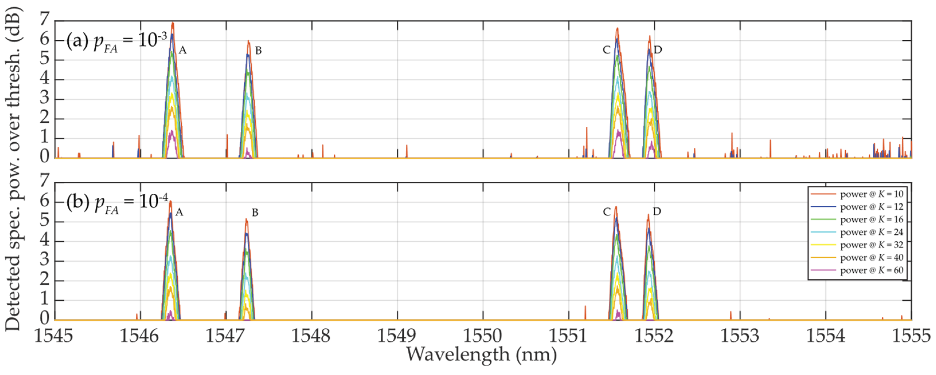
Figure 7.
Statistical characteristics of the additive mixture within sliding windows when K = 10 … 60: (a) mean values μK; (b) standard deviation values σK.
Figure 7.
Statistical characteristics of the additive mixture within sliding windows when K = 10 … 60: (a) mean values μK; (b) standard deviation values σK.
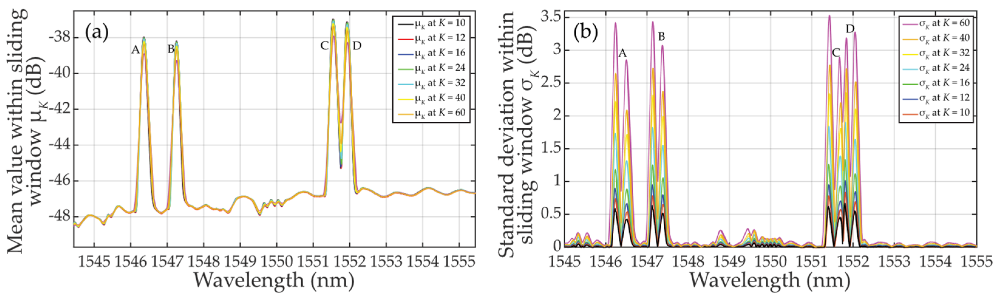
Figure 8.
Concept of the statistical threshold detector of FBG power spectra peaks level with an asymmetric one-sided K/2-size sliding window.
Figure 8.
Concept of the statistical threshold detector of FBG power spectra peaks level with an asymmetric one-sided K/2-size sliding window.

Figure 10.
Results of dynamic statistical threshold detection of the wideband (A, ... , D) FBGs with different power levels, pFA ≈ 10—3 and K/2 = 4 ... 30.
Figure 10.
Results of dynamic statistical threshold detection of the wideband (A, ... , D) FBGs with different power levels, pFA ≈ 10—3 and K/2 = 4 ... 30.

Figure 11.
Illustration of value differences of the wideband (A, ... , D) FBGs when K/2 = 8 … 30: (a) pFA ≈ 10—3; (b) pFA ≈ 10—4.
Figure 11.
Illustration of value differences of the wideband (A, ... , D) FBGs when K/2 = 8 … 30: (a) pFA ≈ 10—3; (b) pFA ≈ 10—4.
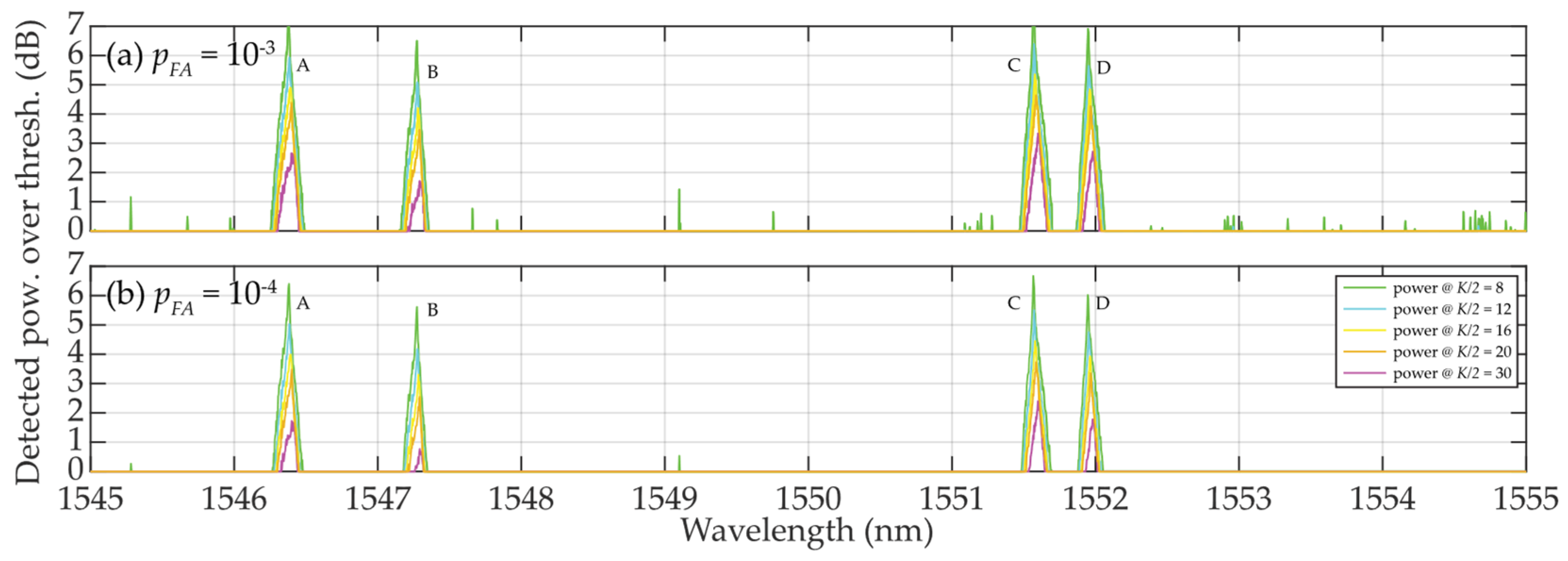
Figure 12.
Calculated statistical characteristics of the FBG power spectra levels plus background noise within sliding windows when K = 10 … 60: (a) mean values μK; (b) standard deviation values σK.
Figure 12.
Calculated statistical characteristics of the FBG power spectra levels plus background noise within sliding windows when K = 10 … 60: (a) mean values μK; (b) standard deviation values σK.
Disclaimer/Publisher’s Note: The statements, opinions and data contained in all publications are solely those of the individual author(s) and contributor(s) and not of MDPI and/or the editor(s). MDPI and/or the editor(s) disclaim responsibility for any injury to people or property resulting from any ideas, methods, instructions or products referred to in the content. |
© 2024 by the authors. Licensee MDPI, Basel, Switzerland. This article is an open access article distributed under the terms and conditions of the Creative Commons Attribution (CC BY) license (http://creativecommons.org/licenses/by/4.0/).
Copyright: This open access article is published under a Creative Commons CC BY 4.0 license, which permit the free download, distribution, and reuse, provided that the author and preprint are cited in any reuse.


