
Submitted:
23 February 2024
Posted:
26 February 2024
You are already at the latest version
Abstract
Crop yield estimation supported by satellite remote sensing data can provide expeditious and strategic information for farmers’ decision-making. Most recent forecasting methods have indicated a promising pathway based on machine learning algorithms. However, validation performances, demand for big data and their inherent inexplicability have not yet consolidated a substantial differential to replace methods based on simpler and more understandable models. This paper proposes an approach based on simple linear models fitted from vegetation indices (VIs) assessed at regular intervals of time series derived from MODIS satellite images, aiming to forecast cotton yields in representative areas of the Brazilian Cerrado. Data from 281 commercial production plots were taken to train (167 plots) and test (114 plots) linear regression models relating seed cotton yield and nine well-known VIs averaged in 15-days intervals. Among the evaluated VIs, EVI (Enhanced Vegetation Index) and TVI (Triangular Vegetation Index) showed the lowest root mean square errors (RMSE) and the highest determination coefficients. The best periods for in-season yield prediction were from the 90-105 to 135-150 days after sowing (DAS), i.e. phenological phases corresponding to boll development, open boll and fiber maturation, with lowest RMSE of about 750 kg ha-1 and R2=0.70. The best forecasts for early crop stages were provided by models at the peaks (maximum value of the VI time-series) for EVI and TVI, which occurred around 80-90 DAS. The proposed approach makes the yield predictability more inferable along the crop time series just by providing sowing dates, contour maps and its respective VIs.
Keywords:
remote sensing
; yield prediction
; cotton
; Brazilian Cerrado
1. Introduction
Cotton is an important cash crop in Brazil, which is the world's fourth largest producer and the second largest exporter, with 1.66 million hectares cultivated in the 2022-2023 season and a total lint production of 3.03 million tons [1]. Most of the cotton has been cultivated in the Brazilian Cerrado, a biome typically characterized by flat and arable lands with good rainfall (750 to 2000 mm/year for the whole Cerrado area [2]), under a highly mechanized, rainfed (92% of the total production [3]), intensive double crop production system, generally cultivated from January to July after soybean [4]. The main cotton producing states have been Mato Grosso and Bahia, which together account for around 90% of the total cotton produced in Brazil [5].
Estimating in-season cotton yield over large areas at a regional or national level provides critical information for farmers, policymakers, governments, crop insurers and commodity traders. Yield estimations are generally performed by a combination of field surveys, remote sensing, statistical regression and crop simulation models [6,7]. Particularly for farmers, the mid-season crop forecasting is very important for management, harvesting, storage and transport logistics decisions and also for planning the next crop [8,9]. Forecasting cotton yield in advance (i.e. before 90-100 days after sowing) is a valuable management information for making viable corrective interventions, such as adjustments to the application of planned inputs (top dressing fertilizer, growth regulators and others), comparing predicted to the expected or historical yields of specific fields.
Although crop yield models have shown adequate performances in field-scale estimations, their applications in large areas are difficult due to the huge amount of data and computational processing costs [10]. To overcome this limitation, statistical regression models such as multiple linear regression and machine learning techniques have been applied to combine spectral indices obtained from satellite data and climate variables, at regional or national level [10-12]. In Table 1 is shown several cotton yield estimation studies using statistical regression models, or crop models combined with remote sensing at regional and field scale under different platforms (satellite, airplane, unmanned aerial vehicle (UAV) or ground sensors) in different countries. Three of these studies developed regression models (Random Forest, among other techniques) to predict cotton yield at a regional scale in China [10], India [11] and Australia [12] from satellite-derived vegetation indices (VIs) and climate variables as covariates. They included precipitation, temperature, evapotranspiration, vapor pressure, soil moisture, among other climate variables. Hundreds of data instances from thousands of hectares in different farm fields over many crop years were used to train and test model performances, which resulted in root mean square errors (RMSE) for seed cotton yield of 157 kg ha-1 [10], 375 kg ha-1 [11] and 976 kg ha-1 [12], in China, India and Australia, respectively.
Simple linear regression models have been developed to predict cotton yield using only satellite-derived vegetation indices as independent variables [13-16], unmanned aerial vehicle (UAV) [17-20], airplane [21] and ground sensor [22]. If on the one hand VIs by themselves have shown some limitations for describing the complex relationships among production, plant physiology, climate, soil nutrition, soil water parameters, pest and disease infestation, crop design and management characteristics [10], on the other several studies have indicated that crop yield can be predicted with relatively good accuracies with this approach [7,23,24]. Just to give an idea of the average magnitude assessed from the summary review shown in Table 1, the average of RMSEs for seed cotton yield for the linear regressions was close to that one assessed by using machine learning techniques and crop model approaches, which indicates linear regression models as potentially advantageous since they operate with a smaller set of well-defined (independent) variables, fewer data manipulation and smaller amounts of instances compared to the other approaches. Moreover, the greater mathematical explainability inherent in linear equations for specific satellite products, VI and crop phenological stage can be directly transferred and/or easily adapted to other locations, allowing clearer understandings and comparisons among different models.

Table 1.
A review of previous studies for estimation of seed cotton yield using remote sensing.
| Reference | Country | Plot | Area | Model | RS source$ | Regression | RMSE## | R2 |
|---|---|---|---|---|---|---|---|---|
| ha | Aproach& | Model# | kg ha-1 | |||||
| [10] | China | 355 | - | CV/RS | Modis/Sentinel | LSTM, SVM, RF | 375 | 0.65 |
| [42] | EUA | 12 | 150 | CM/RS | Spectroradiometer | 468 | - | |
| [13] | USA | 3 | 188 | RS | Modis/Landsat | LR | 673 | 0.52 |
| [14] | USA | - | - | RS | Modis | LR | - | 0.16 |
| [11] | India | - | - | CV, RS | Modis | RF | 157 | 0.69 |
| [12] | Australia | 253 | - | CV, RS | Landsat | RF | 976 | - |
| [17] | USA | 1 | 5 | RS | UAV | MLR | 261 | 0.87 |
| [36] | USA | 805 | 0,65 | RS | UAV | ANN, RF | - | 0.72 |
| [39] | USA | 1 | 57 | RS | Modis/Landsat | 463 | 0.84 | |
| [43] | USA | - | - | EM/RS | Sentinel | - | - | |
| [18] | USA | 2550 | 6 | RS | UAV | LR | 550 | 0.92 |
| [37] | Brazil | 1 | 90 | RS | Optical sensor | decision trees | - | 0.81 |
| [40] | USA | - | 73 | RS | Landsat | ANN | 375-470 | 0.71 |
| [38] | USA | 2 | 120 | RS | Landsat | exponential | 481 | 0.81 |
| [19] | Australia | 90 | 7 | RS | UAV | LR and quadradic | - | 0.75 |
| [15] | USA | 949 | - | RS | Modis | LR | - | 0.48 |
| [16] | USA | 24 | 0,2 | RS | NASA data | LR | - | 0.85 |
| [21] | USA | 48 | 1,5 | RS | Airborne | LR | - | 0.47 |
| [22] | USA | 44 | 5,3 | RS | Spectroradiometer | LR | - | 0.89 |
| &CV: Climate Variables, RS: Remote Sensing, CM: Crop Model, EM: Ecosystem Model; %RS: Remote Sensing; | ||||||||
| UAV: Unmanned Aerial Vehicle; #LSTM: Long Short-Term Memory; SVM: Support Vector Machine; RF: Random Forest; | ||||||||
| LR: Linear Regression, MLR: Multiple Linear Regression, ANN: Artificial Neural, Network; | ||||||||
| ##Root Mean Square Error of seed cotton yield. | ||||||||
The present study evaluates the potential of using simple linear models for correlating yield and satellite-derived VIs from EOS-MODIS (Moderate Resolution Imaging Spectroradiometer) to forecast in-season cotton yield in the Brazilian Cerrado. Reflectance time-series from several MODIS spectral bands were extracted for assessing 15-day interval averages (from sowing to harvest) of well-known VIs. These regular interval averages were evaluated as predictors (independent variables) in linear regression models for estimating cotton yield. The on-farm research was carried out in 281 commercial farm fields under different cotton yields, sowing dates and geographically sparse (with enough geographic information for delimitating the cotton farm field contour).
2. Materials and Methods
2.1. Experimental areas and dataset
The regression models were trained and tested using data from 281 commercial cotton farm fields (hereinafter referred to as plots) in the states of Mato Grosso (125 plots), Goiás (83 plots) and Bahia (73 plots) for the growing seasons of 2016 to 2022. Data from 2016, 2017 and 2018 seasons were obtained from surveys carried out by the Mato Grosso Cotton Institute [25,26] and the Brazilian Agricultural Research Corporation [27], and from cotton farmers in seasons 2019 to 2022. In Figure 1 is depicted the spatial distribution of the 281 plots. Most plots in Mato Grosso, Goiás and Bahia were located at the west, south and west parts of the states, respectively.
The dataset includes information of seed cotton yield for the whole plot (kg ha-1), plot area (ha), cultivar, plant line spacing (m), seed population (seed ha-1), sowing date and water management (irrigated or rainfed). In Figure 2 are shown histograms for some of these parameters. The average seed cotton yield assessed for the 281 plots was 4,209 kg ha-1, ranging from 694 kg ha-1 to 7,361 kg ha-1 (Figure 2a). Low yield plots were located in Mato Grosso and Goiás under rainfed production in seasons 2016 and 2022, something particularly caused by drought or irregular rainfall distributions during these crop seasons [28]. Most of the high yield plots was located in Bahia under central pivot irrigation and in Mato Grosso and Goiás during years with good rain distributions (2017 and 2018). Only 20% of the plots (56) were cultivated under irrigation, being all of them in Bahia and Goiás, whereas the remaining (80%) were under rainfed production (225 plots). Plots in Mato Grosso (125) were all under rainfed production. Plant line spacing used was mostly 0.9 m with average seed linear density of 10 seed m-1, resulting in average population of 111,111 seed ha-1. The average area of the plots was 188 ha (Figure 2c) and average cotton cycle was 196 days (Figure 2d).
Daily accumulated precipitations, maximum and minimum air temperatures data were obtained for each plot by mean of the Brazilian agrometeorological monitoring system (web application) AGRITEMPO [29], by taking the closest climate station to each plot and downloading the daily climate data from 0 to 180 days after sowing (DAS). The data were then averaged for month 1 (0-30 DAS) to 6 (150-180 DAS) and then correlated to the observed yield only to evaluate the effects of the climate variables on yield and to help explain possible bias between observed and predicted yields.
2.2. Satellite data acquisition and preprocessing
With geographic coordinates of all plots, contour maps (kml format) were generated using the Google Earth Pro (Google, Mountain View, CA), which were then converted in shapefile format files using the QGIS software [30]. The spectral reflectance bands and VIs time-series were obtained from the EOS-MODIS MCD43A4 V6.1 Nadir Bidirectional Reflectance Distribution Function Adjusted Reflectance (NBAR) product, which provides smoothed daily data, with a spatial resolution of 500 meters, corrected based on the 16-day compositions with selection of the best pixels (maximum value composite) in that time period to compose the new interval-mediated time series. The spectral bands in this product are blue (0.459-0.479 m), green (0.545-0.565 m), red (0.62-0.67 m), near infrared-NIR (0.841-0.876 m), short wave infrared-SWIR1 (1.23-1.25 m), SWIR2 (1.628-1.656 m) and SWIR3 (2.105-2.155 m). Google Earth Engine (GEE) platform, by mean of its JavaScript code editor, was programmed to extract the time-series, select the pixels within the plot contour area and generate the average values for each spectral reflectance band for each date from sowing to harvesting. The reflectance image and the time-series graph were visually checked before exporting the representative time-series (comma-separated values - csv format) of each plot. A buffer command of 250 m was applied in the GEE code to avoid pixels located at the plot boundary.
Spectral bands were then combined in an Excel® worksheet and the VIs were calculated, averaged in 15-days intervals from 0 to 240 DAS and correlated to cotton yield for the mutually exclusive intervals. Table 2 lists the VIs evaluated and their definitions. A subset of plots (167) was randomly selected (balanced by yield) and used for generating the regression models (training set) and the remaining dataset (114 plots) was used for the independent model validation (test set), i.e., a well-known cross-validation method set as 60%-40% (train-test). Linear regression models were fitted for each combination of VI (Table 2) and time interval. Model’s accuracies were measured by the Root Mean Square Error (RMSE) and determination coefficient (R²) estimated from the test set.
3. Results and Discussion
Examples of MODIS images (NIR band) and time-series of all spectral reflectance bands are shown in Figure 3 for a plot with very low cotton yield (1,665 kg ha-1 in season 2016; Figure 3a, left) and high yield (4,965 kg ha-1 in season 2017; Figure 3a, right). The original smoothed daily time-series are shown in Figure 3b and 15-days averaged time-series in Figure 3c. Reflectance data are plotted in a logarithmic scale for better comparisons among the spectral bands. In general, lower reflectance values (greater absorption of electromagnetic radiation) are observed for the blue, red and green bands, due to the absorption of these light wavelengths by leaves through photosynthesis; higher reflectances in this range can be associated to plant stresses caused by biotic and/or abiotic factors. The spectral range between 0.4 and 0.7 m (visible region) is the photosynthetically active radiation (PAR) that is the most efficient portion of the electromagnetic spectrum used by plant for photosynthesis. Healthy plants present high light absorption in the visible range (0.4-0.7 m) mainly by the leaf pigments like chlorophyll and carotenoids, relatively high reflectance in the NIR range (0.7-1.1 m) due to leaf and cell structure scattering effects, and relatively low reflectance in the SWIR range (1.1-2.5 m) due to water and chemicals into the leaf structure [31,32]. For an actual instance, the low cotton yield (left graph in Figure 3) was mainly caused by low precipitation (water stress) in the 2016 season [28], which is noted by slight increases in red and blue reflectances (lower absorbance by cotton plants), specially between 70 to 170 DAS, and decreasing NIR reflectance, as compared to the high yield plot (right).
In Figure 4a is shown spectral bands time-series averaged for five classes of cotton yield (< 3, 3-3.75, 3.75-4.5, 4.5-5.25, > 5.25 ton ha-1). Reflectance of NIR and SWIR1 increased with increasing cotton yield, while red, blue, SWIR2, SWIR3 reflectance decreases as yield increased, specially from about 60-80 DAS to harvesting, as can be seen by the correlation coefficients (r) between cotton yield and reflectance shown in Figure 4b. The green band reflectance was higher than red and blue, as expected, but its relationship with yield was not graphically evident (Figure 4a). Best correlations between the spectral reflectance bands and cotton yield were obtained for NIR, SWIR1 (positive), SWIR3, red, SWIR2 and blue (negative) (Figure 4b). These data, obtained using broadband wavelengths satellite sensors are similar to others obtained with narrow band ground measurements by spectroradiometers. For instance, Thenkabail et al. [33] obtained negative correlation between cotton biophysical parameters (leaf area index, wet biomass, plant height and crop yield) and reflectance for wavelengths between 350 nm to about 700 nm (visible light) and positive correlations for wavelengths from about 730 nm to 1050 nm (NIR to part of the SWIR range).
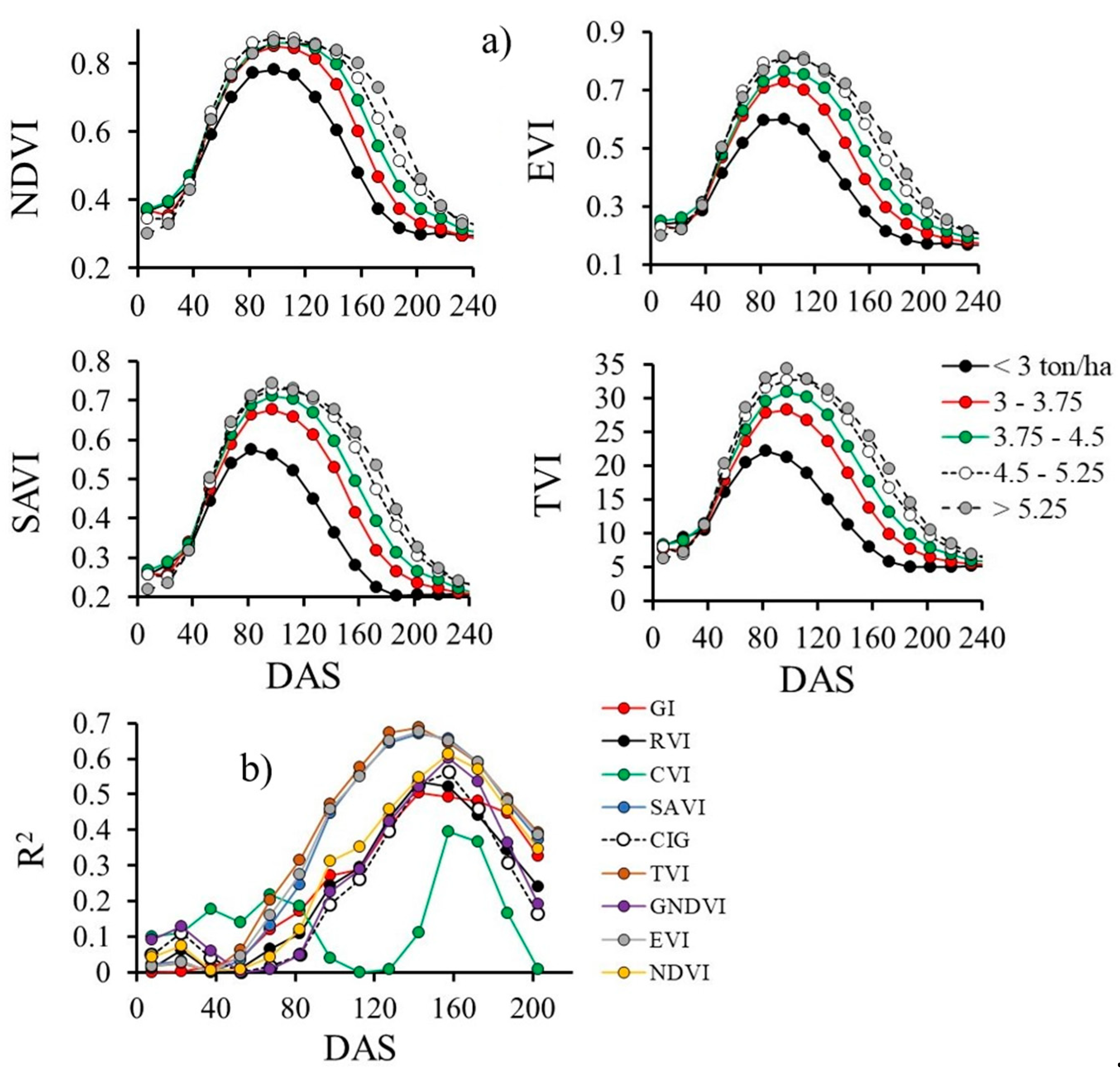
The nine vegetation indices (Table 2) were taken as independent variables to fit simple linear regression models to predict cotton yield using the training dataset (167 plots) for each 15-days interval. Figure 5b shows the determination coefficients (R2) obtained for these VIs and DAS intervals. The highest R2 were provided by the TVI (0.69), EVI (0.68), SAVI (0.67) and NDVI (0.61) for intervals between 120 and 165 DAS, which are in the cotton late-season stage of development (open boll to defoliation). Time-series for these VIs averaged for different yield classes are shown in Figure 5a. In general, there was a saturation trend for all VIs at the peak of time-series for the highest yield classes, and this effect was more pronounced for NDVI, agreeing with other studies that show NDVI saturation at high amounts of green biomass or high leaf area index [34,35].
For the training dataset, TVI, EVI and SAVI produced the highest determination coefficients for cotton yield forecasts, indicating a good potential for in-season cotton yield estimations from these VIs. Table 3 presents the linear regression models for the four VIs with the highest R2 for different 15-days intervals, from 75-90 to 180-195 DAS, and also for 75-195 DAS (average from 75 DAS to about harvesting) and the maximum VI value along the season (denoted as peak). In Figure 6 is shown the relationships between cotton yield and TVI for different DAS intervals. Although highest R2 (0.73) were provided by the interval of 75-195 DAS for the TVI (Figure 6) and also for the other VIs (Table 3), such equations would only be useful at the end of the season, since data needs to be accumulated until 195 DAS before averaging them. For in-season forecasts, the best models were obtained from 105-120 DAS to 165-180 DAS; nevertheless 150-165 and 165-180 DAS intervals are also too close to the end of season and they likely do not have any practical for decision making by farmers. Forecasts based on VI peaks have been used in several studies for in-season yield estimates [14,36]. In the present study the peak models presented R2 lower than for 105-120 to 165-180 DAS (Table 3), but higher than 90-105 DAS, which mean good potential for earlier in-season forecasts, since the time-series peak values for TVI, EVI, SAVI and NDVI occurred at about 80 to 100 DAS, as can be seen in Figure 5.
Figure 5.
MODIS satellite average time-series of NDVI, EVI, SAVI and TVI for five cotton yield classes (a) and determination coefficients (R2) of linear correlations between cotton yield and 9 vegetation indices (Table 2) for the different 15-days DAS (Days After Sowing) classes, for the training dataset (167 plots).
Model estimates for cotton yields using TVI equations (Table 3) compared to observed yields with their respective RMSE are shown in Figure 7; Figure 8 displays RMSE (Figure 8a) and R2 (Figure 8b) variations with DAS intervals for the four best VIs. Lowest RMSE and highest R2 were provided by EVI and TVI for 90-105 to 135-150 DAS (four DAS intervals) allowing in-season yield forecasting with RMSE of about 750 kg ha-1 (Figure 8a). Averaged VIs for 75-195 DAS and peak models showed similar RMSE values to the best models (EVI, TVI and SAVI) for 15-days intervals (90-105 to 135-150 DAS) (Figure 8c), but for EVI the peak model showed the lowest RMSE (726 kg ha-1). The average yield predictions for the 114 testing plots are shown in Figure 8d for 105-120 DAS, 75-195 DAS and peaks. The average observed yield (for the 114 plots) was 4,372 kg ha-1 (dotted horizontal line in Figure 8d) and most of the linear models tend to overestimate yield (about 160 kg ha-1 in average). In general, there were tendencies of yield overestimation for the lower yield plots and underestimation for the higher yield plots, as can be seen in Figure 7 for TVI, but the 75-195 DAS model seems to reduce such bias. Although NDVI provided the closer average yield forecast, for the 114 plots, to the measured average yield (Figure 8d) its RMSE was much higher than the other VIs (EVI, TVI and SAVI) for all intervals between 75 and 165 DAS. Thus, the best performances were obtained with EVI and TVI for 105-120, 120-35 and 135-150 DAS intervals. If an earlier prediction is required, the 90-105 DAS or peak models are preferred, since RMSE for DAS 75-90 DAS and earlier DAS were too high and R2 were inexpressive.
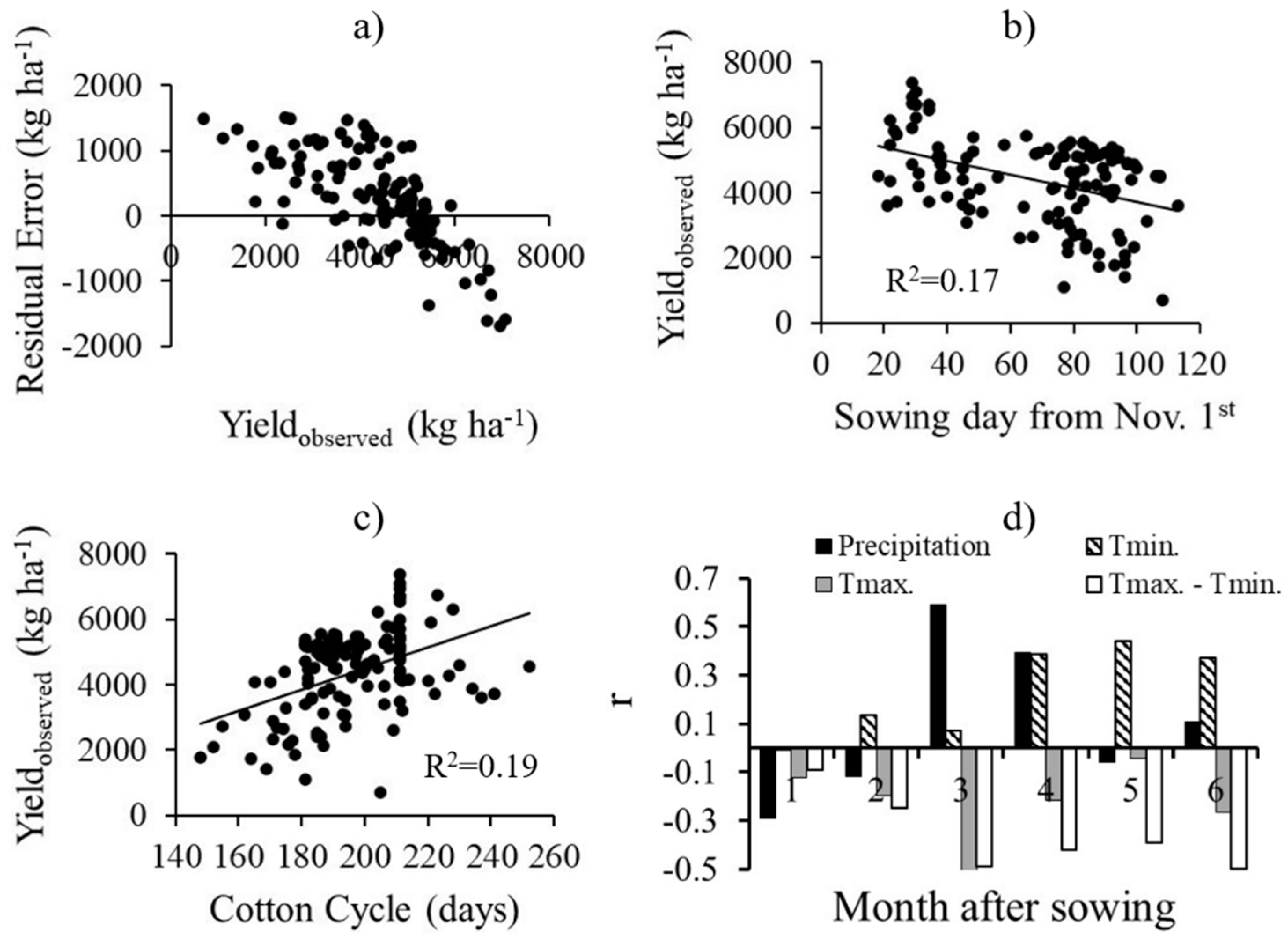
The overestimation trend observed for low yield plots and underestimation for high yields (Figure 7) can be better evaluated correlating the residual error (yieldestimated - yieldobserved; estimated by the peak model with TVI) with the observed yield of each plot (Figure 9a), where negative residual errors (underestimation) are verified for yields higher than about 4,000 kg ha-1 and positive (overestimation) for lower yield values. Several factors may contribute and explain the low and high yield plots, as the climate conditions, soil type, soil fertility, diseases, cultivars and others. Nevertheless, in rainfed cotton production one of the main driven factors that affects yield has been the climatic condition, particularly precipitation and temperature variations along the season. Therefore, the sowing date and cycle duration, established based on the recommended cultivar and local climatic patterns, are impacted by water demands and temperature for each cotton development stages and consequently the expected cotton yield. For the testing dataset, the earliest sowing date was November 19, so observed yield was correlated to sowing after November 1st as a proxy for sowing data, independent of the year (Figure 9b), showing a negative influence on yield. The cotton cycle duration, which is basically defined by the cultivar used, showed a positive correlation with yield (Figure 9c). These two parameters are intrinsically related to the climatic conditions and both influenced the observed yields. There is a trend of increasing yield for earlier sowing day and for longer cotton cycle duration.
The best correlations between monthly accumulated precipitation and yield occurred in the third and fourth months after sowing (r=0.59 for 60-90 DAS and 0.39 for 90-120 DAS; Figure 9d) that is the cotton mid-season corresponding to the canopy closure until flowering and boll development stages. In the first month, rainfall showed an adverse effect on yield (r=-0.29) since high-intensity rainfall in the very early season can damage the germination process. Monthly averaged maximum and minimum temperatures and their differences (Tmax-Tmin) also influenced yield mainly after the third month (r=-0.49).
Figure 9.
Relationships between the residual error (yieldestimated-yieldobserved; estimated by TVI peak model) and observed cotton yield (a), observed yield and sawing day from November 1st (b), observed yield and cotton cycle (c), and correlation coefficients (r) between observed yield and monthly accumulated precipitation, monthly averaged minimum (Tmin) and maximum (Tmax) temperatures, and Tmax-Tmin (d) for month 1 to 6 after sowing.
Several studies as those included in Table 1 evaluated the best period for acquiring Satellite and UAV images or ground measurements for best cotton yield predictions. Some works have used a single date image and others have evaluated images at specific phenological stages or complete time-series data. Table 4 summarizes the best periods, in DAS, inferred from the papers listed in Table 1. The best correlations between cotton yield and the VIs varied from the flowering and boll development period [12,18,22,37,38,39] to boll opening, maturation and defoliant application [10,15,16,17,19,21,40,41], with the latter in agreement with the results obtained in the present study. Particularly, the study carried out by Lang et al. [10] in 355 plots of cotton cultivated from 2012 to 2019 in Xinjiang Province, China, showed very similar results to ours, with lowest RMSE and highest R2 for the fourth and fifth months after sowing (90-120 to 120-150 DAS).
Several studies as those included in Table 1 evaluated the best period for acquiring Satellite and UAV images or ground measurements for best cotton yield predictions. Some works have used a single date image and others have evaluated images at specific phenological stages or complete time-series data. Table 4 summarizes the best periods, in DAS, inferred from the papers listed in Table 1. The best correlations between cotton yield and the VIs varied from the flowering and boll development period [12,18,22,37,38,39] to boll opening, maturation and defoliant application [10,15,16,17,19,21,40,41], with the latter in agreement with the results obtained in the present study. Particularly, the study carried out by Lang et al. [10] in 355 plots of cotton cultivated from 2012 to 2019 in Xinjiang Province, China, showed very similar results to ours, with lowest RMSE and highest R2 for the fourth and fifth months after sowing (90-120 to 120-150 DAS).
The best forecasting models for mid to late-season (90 to 150 DAS) for a regional scale can be useful as advance information for institutions as commodity traders, policymakers and governments, and in some instance, for farmers, mainly regarding their logistics and for planning the next crop season (for example, planning plot fertilizer reposition for the next crop based on the previous crop nutrients exportation). For some in-season interventions, as topdressing fertilizer applications, some forecasting models may be impractical, since most of the topdressing fertilizers (macro and micronutrients) are commonly applied before 100 DAS. Nevertheless, earlier prediction using peak models still provides an opportunity window for topdressing fertilizer intervention, since at about 80 DAS around 45%, 50% and 80% of sulfur, potassium and nitrogen, respectively, have been absorbed by cotton plants [42].
4. Conclusions
The forecasting approach based on simple regression models and time series intervals for cotton yield using the Modis product MCD43A4 V6.1 allowed in-season prediction with RMSE of about 750 kg ha-1 at a regional scale in three cotton-producing states at the Brazilian Cerrado. This RMSE was higher than the ones obtained by Prasad et al. [11] and Lang et al. [10] for seed cotton yield prediction at regional scales in India and China, respectively, but close to the RMSE obtained by Filippi et al. [12] in Australian fields. The approach is simple and can be easily applied to predict seed cotton yield at farm, region and country levels. One limitation of the approach is the coarse spatial resolution of the Modis product, which restricts its use only for large commercial plots, such those in crop production system in the Brazilian Cerrado.
Among the nine VIs evaluated, EVI and TVI were the best individual predictors. Accuracies, evaluated by mean of RMSEs, were very low up to 75 DAS, which constitute a limitation to the application of such approach to estimate cotton yield during the first stages of cotton development. Best in-season prediction was provided by 15-days intervals between 90-105 to 135-150 DAS that corresponds to part of the mid-season to late season stage of development (boll development, open boll and fiber maturation). Best forecasts for earlier stages (below 90-105 DAS class) were provided by the model fitted for peaks with EVI and TVI, which occur around 80-90 DAS.
Future validation experiments should evaluate the accuracies and usefulness of some models in the next coming cotton seasons at different sub-regions, including their abilities to predict cotton net production in a whole farm, state and at regional and country levels. Model’s usefulness at farm level for some management interventions (within-season topdressing fertilizer application or planning reposition for the next crop based on exported nutrients, for instance) requires due caution and/or other validations.
The proposed approach can be extended to corn, which is widely cultivated as second harvest in the Brazilian Cerrado and likely to soybean (cultivated in the rainy season and with much more cloud interference in the satellite images) that is the main first crop cultivated in Brazil.
Author Contributions
Conceptualization, Carlos Vaz and Flávio Silva; Data curation, Rafael Galbieri, Jean Belot, Márcio de Souza, Fabiano Perina and Sérgio das Chagas; Formal analysis, Daniel Siqueira, Carlos Vaz and Flávio Silva; Investigation, Daniel Siqueira, Carlos Vaz and Flávio Silva; Methodology, Daniel Siqueira, Carlos Vaz, Flávio Silva, Ednaldo Ferreira and Júlio Franchini; Resources, Rafael Galbieri, Jean Belot, Márcio de Souza, Fabiano Perina and Sérgio das Chagas; Software, Flávio Silva and Eduardo Speranza; Supervision, Carlos Vaz; Validation, Daniel Siqueira and Carlos Vaz; Writing – original draft, Daniel Siqueira and Carlos Vaz; Writing – review & editing, Carlos Vaz, Ednaldo Ferreira, Eduardo Speranza, Júlio Franchini, Rafael Galbieri, Jean Belot, Márcio de Souza and Fabiano Perina.
Acknowledgments and Funding
The authors acknowledge the financial support from the Brazilian Agricultural Research Corporation (EMBRAPA) and the Mato Grosso Cotton Institute (IMAmt) through a joint cooperation project (30.21.90.03) and thank the farmers in Mato Grosso, Bahia, and Goiás who voluntarily provided access to their commercial plots data.
Conflicts of Interest
The authors declare no conflicts of interest.
References
- ABRAPA. Safra Brasil. 2024. Available online: https://abrapa.com.br/dados/ (accessed on 16 February 2024).
- Eiten, G. Cerrado vegetation: vegetation and climate in Brazil. In Pinto, M.N. (Org). Cerrado: characterization, occupation and perspectives (in Portuguese); UNB: Brasília, Brazil, 1993; pp. 17–73. [Google Scholar]
- COTTON BRAZIL, 2024. Market Report, January 19, 2024. Available online: file:///C:/Users/carlos.vaz/Downloads/ABRAPA_COTTON_BRAZIL_REPORT_-_2024_01-1.pdf . (accessed on 16 February 2024).
- Echer, F.R.; Mello, P.R.; Rosolem, C.A. Management of plant growth regulators. In J.L. Belot and P.M.C.A. Vilela (ed.), Best Management Practices for Cotton in Mato Grosso State (in Portuguese), 4th ed.; IMAmt-AMPA: Cuiabá, MT, Brazil, 2020; pp. 312–319. [Google Scholar]
- CONAB. Companhia Nacional de Abastecimento. 2024. Available online: https://www.conab.gov.br/info-agro/safras/serie-historica-das-safras/itemlist/category/898-algodao (accessed on 16 February 2024).
- Basso, B.; Liu, L. Seasonal crop yield forecast: Methods, applications, and accuracies. Adv. Agron. 2019, 154, 201–255. [Google Scholar]
- Li, F.; Miao, Y.; Chen, X.; Sun, Z.; Stueve, K.; Yuan, F. In-season prediction of corn grain yield through PlanetScope and Sentinel-2 images. Agronomy, 2022, 12, 3176. [Google Scholar] [CrossRef]
- Khanal, S.; Kushal, K.C.; Fulton, J.P.; Shearer, S.; Ozkan, E. Remote sensing in agriculture - Accomplishments, limitations, and opportunities. Remote Sens. 2020, 12, 3783. [Google Scholar] [CrossRef]
- Taskiner, T.; Bilgen, B. Optimization models for harvest and production planning in agri-food supply chain: A systematic review. Logistics 2021, 5, 52. [Google Scholar] [CrossRef]
- Lang, P.; Zhang, L.; Huang, C.; Chen, J.; Kang, X.; Zhang, Z.; Tong, Q. Integrating environmental and satellite data to estimate county-level cotton yield in Xinjiang Province. Front. Plant Sci. 2023, 13, 1048479. [Google Scholar] [CrossRef]
- Prasad, N.R.; Patel, N.R.; Danodia, A. Crop yield prediction in cotton for regional level using Random Forest approach. Spat. Inf. Res. 2020, 29, 195–206. [Google Scholar] [CrossRef]
- Filippi, P.; Whelan, M.B.; Vervoort, R.W.; Bishop, T.F.A. Mid-season empirical cotton yield forecasts at fine resolutions using large yield mapping datasets and diverse spatial covariates. Agric. Syst. 2020, 184, 102894. [Google Scholar] [CrossRef]
- Meng, L.; Liu, H.; Ustin, S.L.; Zhang, X. Assessment of FSDAF accuracy on cotton yield estimation using different Modis products and Landsat based on the mixed degree index with different surroundings. Sensors 2021, 21, 5184. [Google Scholar] [CrossRef]
- Johnson, D.M.; Rosales, A.; Mueller, R.; Reynolds, C.; Frantz, R.; Anyamba, A.; Pak, E.; Tucker, C. USA crop yield estimation with MODIS NDVI: Are remotely sensed models better than simple trend analyses? Remote Sens. 2021, 13, 4227. [Google Scholar] [CrossRef]
- Johnson, D.M. A comprehensive assessment of the correlations between field crop yields and commonly used MODIS products. Int. J. Appl. Earth Obs. Geoinf. 2016, 52, 65–81. [Google Scholar] [CrossRef]
- Iqbal, J.; Read, J.; Whisler, D. Using remote sensing and soil physical properties for predicting the spatial distribution of cotton lint yield. Turkish J. Field Crop. 2013, 18, 158–165. [Google Scholar]
- Feng, A.; Zhou, J.; Vories, E.D.; Sudduth, K.A.; Zhang, M. Yield estimation in cotton using UAV-based multi-sensor imagery. Biosyst. Eng. 2020, 193, 101–114. [Google Scholar] [CrossRef]
- Feng, A.; Zhang, M.; Sudduth, K.A.; Vories, E.D.; Zhou, J. Cotton yield estimation from UAV-based plant height. Trans. ASABE 2019, 62, 393–403. [Google Scholar] [CrossRef]
- Ballester, C.; Hornbuckle, J.; Brinkhoff, J.; Smith, J.; Quayle, W. Assessment of in-season cotton nitrogen status and lint yield prediction from Unmanned Aerial System imagery. Remote Sens. 2017, 9, 1149. [Google Scholar] [CrossRef]
- Huang, Y.; Brand, H.J.; Sui, R.; Thomson, S.J.; Furukawa, T.; Ebelhar, M.W. Cotton yield estimation using very high-resolution digital images acquired with a low-cost Small Unmanned Aerial Vehicle. Trans. ASABE 2016, 59, 1563–1574. [Google Scholar] [CrossRef]
- Huang, Y.; Sui, R.; Thomson, J.S.; Fisher, D.K. Estimation of cotton yield with varied irrigation and nitrogen treatments using aerial multispectral imagery. Int. J. Agric. Biol. Eng. 2013, 6, 37–41. [Google Scholar]
- Zhao, D.; Reddy, K.R.; Kakani, V.G.; Read, J.J.; Koti, S. Canopy reflectance in cotton for growth assessment and lint yield prediction. Eur. J. Agron. 2007, 26, 335–344. [Google Scholar] [CrossRef]
- He, Y.; Qiu, B.; Cheng, F.; Chen, C.; Sun, Y.; Zhang, D.; Lin, L.; Xu, A. National scale maize yield Estimation by integrating multiple spectral indexes and temporal aggregation. Remote Sens. 2023, 15, 414. [Google Scholar] [CrossRef]
- Fu, Y.; Huang, J.; Shen, Y.; Liu, S.; Huang, Y.; Dong, J. , Han, W.; Ye, T.; Zhao, W.; Yuan, W. A satellite-based method for national winter wheat yield estimating in China. Remote Sens. 2021, 13, 4680. [Google Scholar] [CrossRef]
- Galbieri, R.; Vaz, C.M.P.; Pessatto-Filho, D.; Crestana, S.; Chitarra, L.G.; Lobo-Junior, M.; Lanças, F.M.; Silva, J.F.V.; Faleiro, V.O.; Sarques, B. Cotton production in Goiás: White mold, fusarium wilt, cultivation system and soil physical attributes (In Portuguese). Circular Técnica, Goiás, AGOPA, Brazil, 2018, 20p.
- Galbieri, R.; Vaz, C.M.P.; Silva, J.F.V.; Amus, G.L.A.; Crestana, S.; Matos, E.S.; Magalhaes, C.A.S. Influence of soil parameters on the occurrence of phytonematodes. In Rafel Galbieri; Jean Louis Belot. (Org.). Phytoparasitic nematodes of cotton in Brazilian cerrados: Biology and control measures (In Portuguese). 1ed. IMAmt Cuiabá, MT, Brazil, 2016. [Google Scholar]
- Instituto Nacional de Meteorologia., 2022. Boletim de Monitoramento Agrícola - Culturas de Verão 21/22, 11(5):1-19. Available online: https://portal.inmet.gov.br/ (accessed on 16 February 2024).
- Perina, F.J.; Bogiani, J.C.; Ribeiro, G.C.; Breda, C.E.; Fabris, A.; dos Santos, I.A.; Seibel, D.P. Survey and management of phytonematodes in cotton in western Bahia, results for season 2016/17. Fundação BA, Bahia, Brazil, Circular Técnica, 2017, 8p.
- AGRITEMPO, 2024. Agrometeorological Monitoring System. Available online: http://www.agritempo.gov.br/agritempo/sobre.jsp?lang=en (accessed on 16 February 2024).
- QGIS Development Team. 2022. QGIS Geographic Information System. Open Source Geospatial Foundation Project. Available online: http://qgis.osgeo.org.
- Chattopadhyay, N.; Shukla, K.K.; Birah, A.; Khokhar, M.K.; Kanojia, A.K.; Nigam, R.; Roy, A.; Bhattacharya, B.K. Identification of spectral bands to discriminate wheat Spot Blotch using in situ hyperspectral data. J. Indian Soc. Remote. Sens. 2023, 51, 917–934. [Google Scholar] [CrossRef]
- Knipling, E.B. Physical and physiological basis for the reflectance of visible and near-infrared radiation from vegetation. Remote Sens. Environ. 1970, 1, 155–159. [Google Scholar] [CrossRef]
- Thenkabail, P.S.; Smith, R.B.; De Pauw, E. Hyperspectral vegetation indices and their relationships with agricultural crop characteristics. Remote Sens. Environ. 2000, 71, 158–182. [Google Scholar] [CrossRef]
- Tesfaye, A.A.; Awoke, B.G. Evaluation of the saturation property of vegetation indices derived from sentinel-2 in mixed crop-forest ecosystem. Spat. Inf. Res. 2020, 1, 109–121. [Google Scholar] [CrossRef]
- Xing, N.; Huang, W.; Xie, Q.; Shi, Y.; Ye, H.; Dong, Y.; Wu, M.; Sun, G.; Jiao, Q. A transformed triangular vegetation index for estimating winter wheat leaf area index. Remote Sens. 2020, 12, 16. [Google Scholar] [CrossRef]
- Shammi, S.A.; Meng, Q. Use time series NDVI and EVI to develop dynamic crop growth metrics for yield modeling. Ecological Indicators, 2021, 121, 107124. [Google Scholar] [CrossRef]
- Ashapure, A.; Jung, J.; Chang, A.; Oh, S.; Yeom, J.; Maeda, M.; Maeda, A.; Dube, N.; Landivar, J.; Hague, S.; Smith, W. Developing a machine learning based cotton yield estimation framework using multi-temporal UAS data. ISPRS J. Photogramm. Remote Sens. 2020, 169, 180–194. [Google Scholar] [CrossRef]
- Baio, F.H.R.; da Silva, E.E.; Martins, P.H.A.; da Silva-Júnior, C.A.; Teodoro, P.E. 2019. In situ remote sensing as a strategy to predict cotton seed yield. J. Biosci. 2019, 35, 1847–1854. [Google Scholar] [CrossRef]
- Meng, L.; Zhang, X.; Huanjun, L.; Guo, D.; Yan, Y.; Qin, L. , Pan, Y. Estimation of cotton yield using the reconstructed time-series vegetation index of Landsat data. Can. J. Remote. Sens. 2017, 43, 244–255. [Google Scholar] [CrossRef]
- Meng, L.; Liu, H.; Zhang, X.; Ren, C.; Ustin, S.; Qiu, Z.; Xu, M.; Guo, D. Assessment of the effectiveness of spatiotemporal fusion of multi-source satellite images for cotton yield estimation. Comput. Electron. Agric. 2019, 162, 44–52. [Google Scholar] [CrossRef]
- Haghverdi, A.; Washington-Allen, R.A.; Leib, B.G. Comput. Electron. Agric. 2018, 152, 186–197. [CrossRef]
- Carvalho, M.C.S.; Ferreira, G.B. Cotton liming and fertilization in the cerrado (in Portuguese). Circular Técnica 92, Embrapa, Campina Grande, PB, Brazil, 2006, 16p.
- Jeong, S.; Shin, T.; Ban, J.; Ko, K.J. Simulation of spatiotemporal variations in cotton lint yield in the Texas high plains. Remote Sens. 2022, 14, 1421. [Google Scholar] [CrossRef]
- He, L.; Mostovoy, G. Cotton yield estimate using Sentinel-2 data and an ecosystem model over the southern US. Remote Sens. 2019, 11, 2000. [Google Scholar] [CrossRef]
- Gitelson, A.A.; Gritz, Y.; Merzlyak, M.N. Relationships between leaf chlorophyll content and spectral reflectance and algorithms for non-destructive chlorophyll assessment in higher plant leaves. J. Plant Physiol. 2003, 160, 271–282. [Google Scholar] [CrossRef]
- Jordan, C.F. Derivation of leaf-area index from quality of light on the forest floor. Ecology 1969, 50, 663–666. [Google Scholar] [CrossRef]
- Vincini, M.; Frazzi, E.; D’Alessio, P. A broad-band leaf chlorophyll vegetation index at the canopy scale. Precis. Agric. 2008, 9, 303–319. [Google Scholar] [CrossRef]
- Huete, A.R. A soil-adjusted vegetation index (SAVI). Remote Sens. Environ. 1988, 25, 295–309. [Google Scholar] [CrossRef]
- Broge, N.H.; Leblanc, E. Comparing prediction power and stability of broadband and hyperspectral vegetation indices for estimation of green leaf area index and canopy chlorophyll density. Remote Sens. Environ. 2001, 76, 156–172. [Google Scholar] [CrossRef]
- Kaufman, Y.J.; Merzlyak, M.N. Use of a green channel in remote sensing of global vegetation from EOS-MODIS. Remote Sens. Environ. 1996, 58, 289–298. [Google Scholar] [CrossRef]
- Huete, A.; Didan, K.; Miura, T.; Rodriguez, E.P.; Gao, X.; Ferreira, L.G. Overview of the radiometric and biophysical performance of the MODIS vegetation indices. Remote Sens. Environ. 2002, 83, 195–213. [Google Scholar] [CrossRef]
- Rouse, J.W. Monitoring vegetation systems in the great plains with ERTS: Proceedings of the Third Earth Resources Technology Satellite-1 Symposium- Volume I: Technical Presentations. NASA SP-351 1974, 309-317.
Figure 1.
Spatial location of the 281 plots cultivated with cotton in the states of Mato Grosso, Goiás and Bahia (typical Brazilian Cerrado biome) used to train (yellow dots) and test the models (blue dots) and three cotton plots zoomed.
Figure 1.
Spatial location of the 281 plots cultivated with cotton in the states of Mato Grosso, Goiás and Bahia (typical Brazilian Cerrado biome) used to train (yellow dots) and test the models (blue dots) and three cotton plots zoomed.
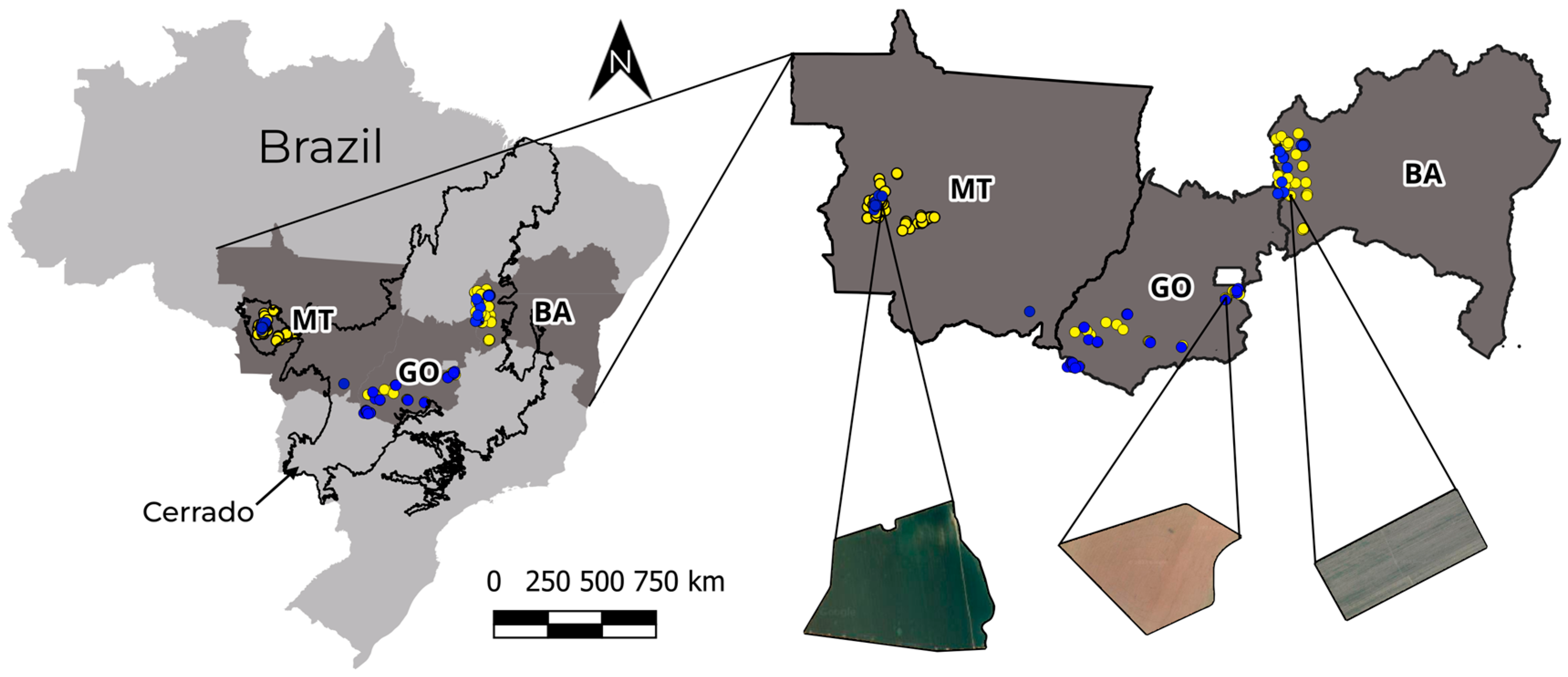
Figure 2.
Frequency distributions of seed cotton yield (a), sowing month (b), plot area (c) and cotton cycle (d) for the 281 commercial plot units.
Figure 2.
Frequency distributions of seed cotton yield (a), sowing month (b), plot area (c) and cotton cycle (d) for the 281 commercial plot units.
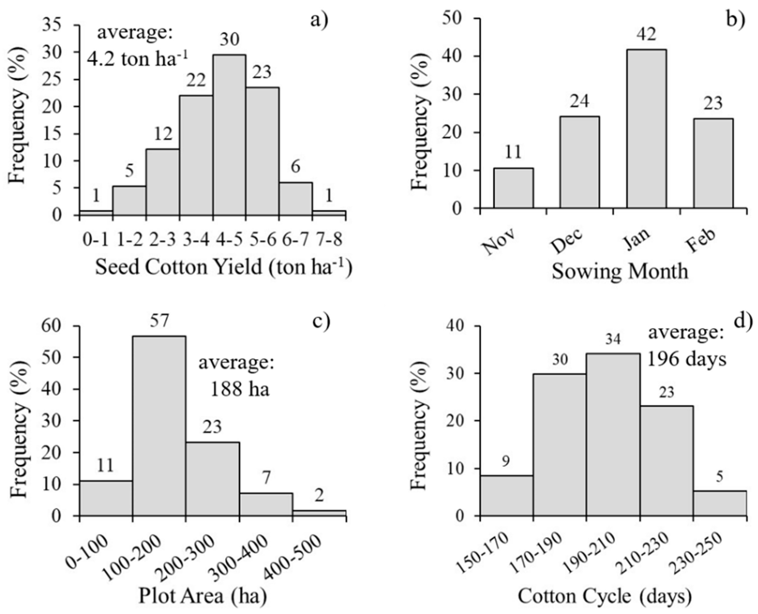
Figure 3.
MODIS product MCD43A4 V6.1 NIR: (a) images obtained for two commercial cotton production plots; (b) original extracted time-series (daily data) for Red, NIR, Blue, Green, and SWIR spectral bands; (c) time series in 15-day interval averages. Plot on left presented low cotton yield on right high cotton yield.
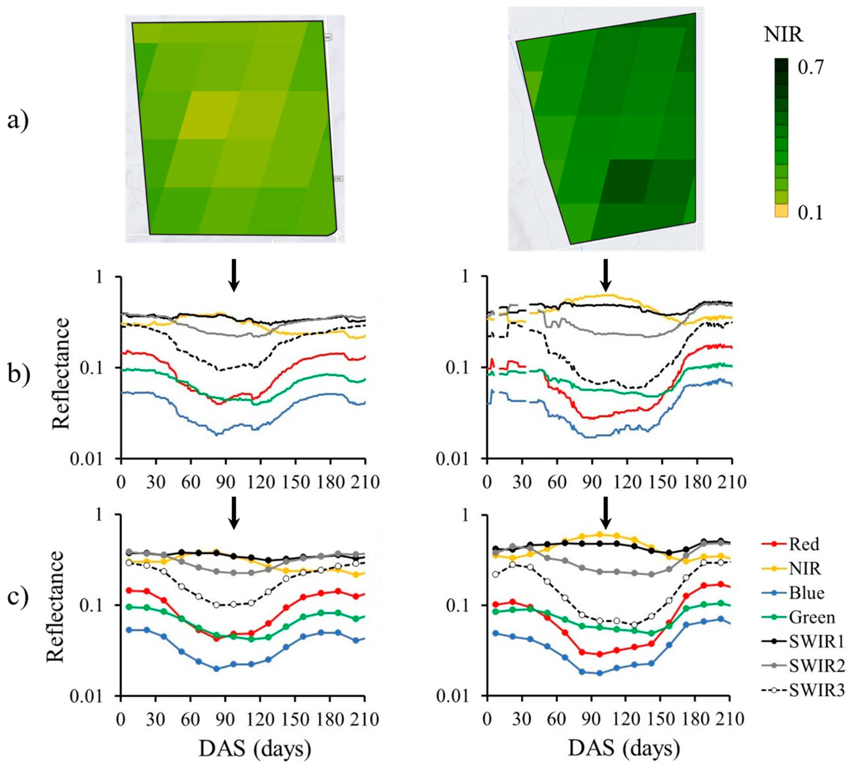
Figure 4.
MODIS satellite average time-series of the seven spectral bands reflectance for five cotton yield classes (a) and linear correlation coefficients (r) between cotton yield and reflectance for the different 15-days DAS (Days After Sowing) classes, for the training dataset (167 plots).
Figure 4.
MODIS satellite average time-series of the seven spectral bands reflectance for five cotton yield classes (a) and linear correlation coefficients (r) between cotton yield and reflectance for the different 15-days DAS (Days After Sowing) classes, for the training dataset (167 plots).
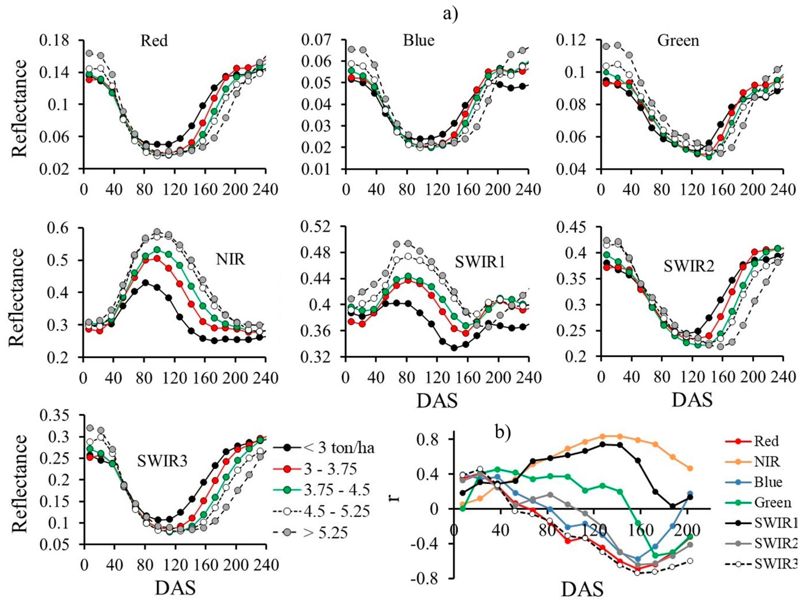
Figure 6.
Linear correlations between TVI and seed cotton for different 15-days DAS for the training dataset, from 75-90 to 180-195 DAS, 75-195 DAS (averaged period) and the time-series peak value. Linear equations shown in Table 3.
Figure 6.
Linear correlations between TVI and seed cotton for different 15-days DAS for the training dataset, from 75-90 to 180-195 DAS, 75-195 DAS (averaged period) and the time-series peak value. Linear equations shown in Table 3.
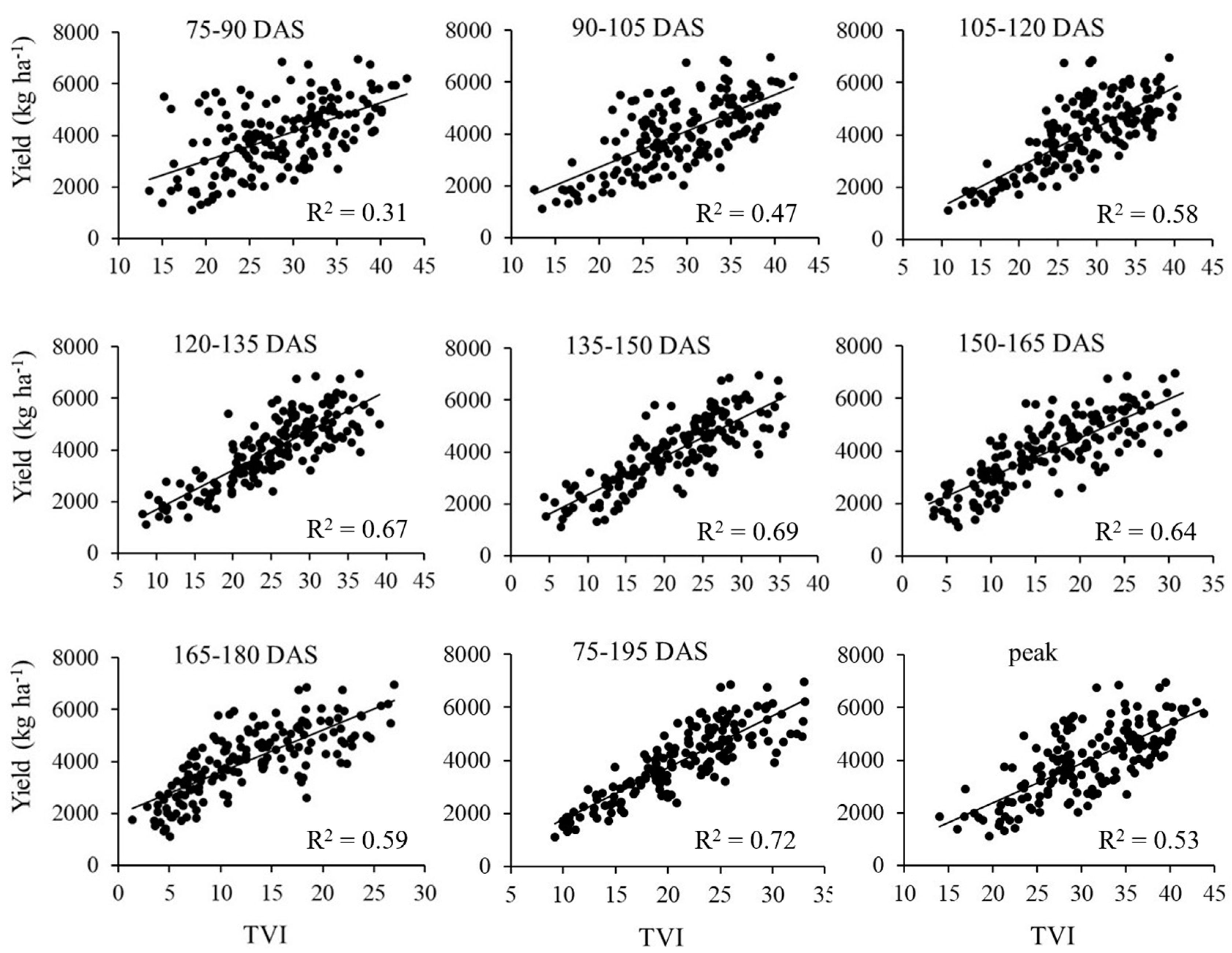
Figure 7.
Comparisons between observed and predicted seed cotton yield for the testing dataset (114 plots) for different 15-days DAS (75-90 to 180-195 DAS), 75-195 DAS (averaged period) and the time-series peak value, and their respective root mean square errors (RMSE), obtained using TVI linear regression models (Table 3).
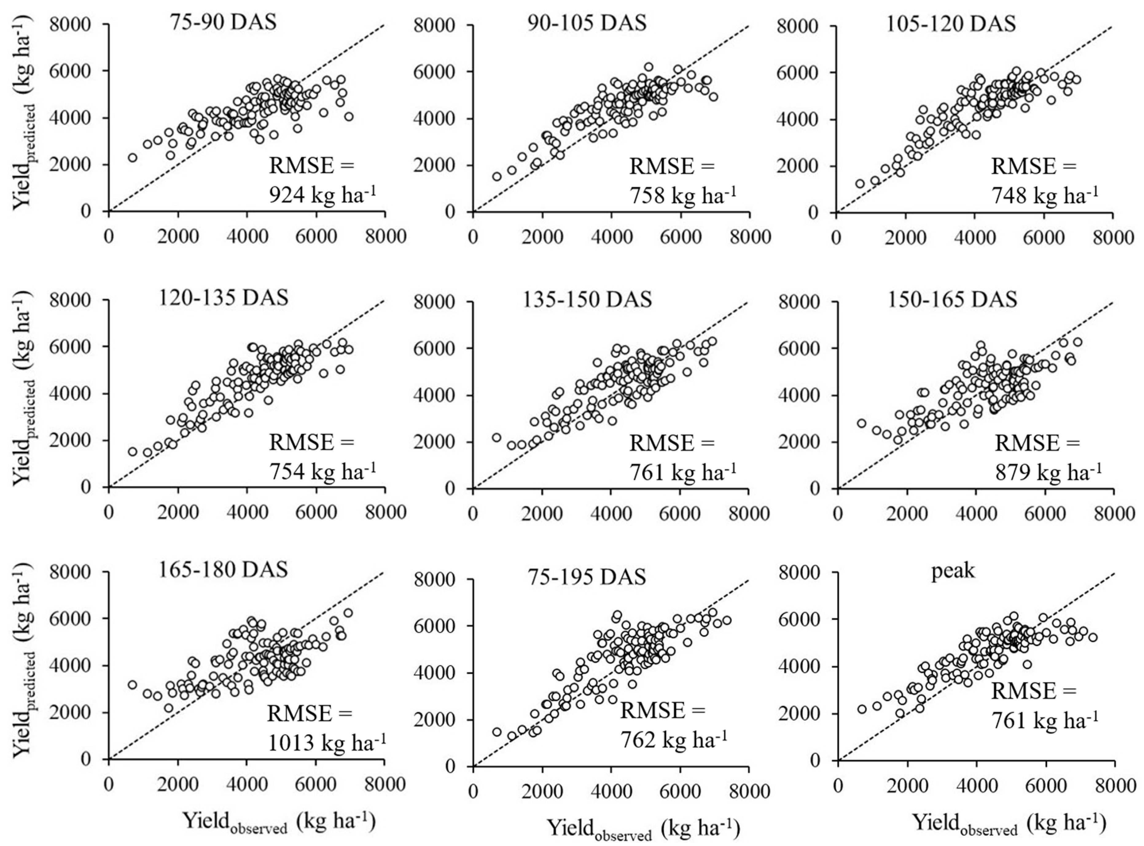
Figure 8.
Root mean square error (RMSE) (a) and linear determination coefficients (R2) (b) between predicted and observed yield for the 114 plots of the testing dataset for different 15-days DAS; comparison of RMSE (c) and predicted yield (d) for 105-120 DAS, 75-195 DAS and peak equations for TVI, EVI, SAVI and NDVI. Doted horizontal line in d) represents the average observed yield for the 114 plots.
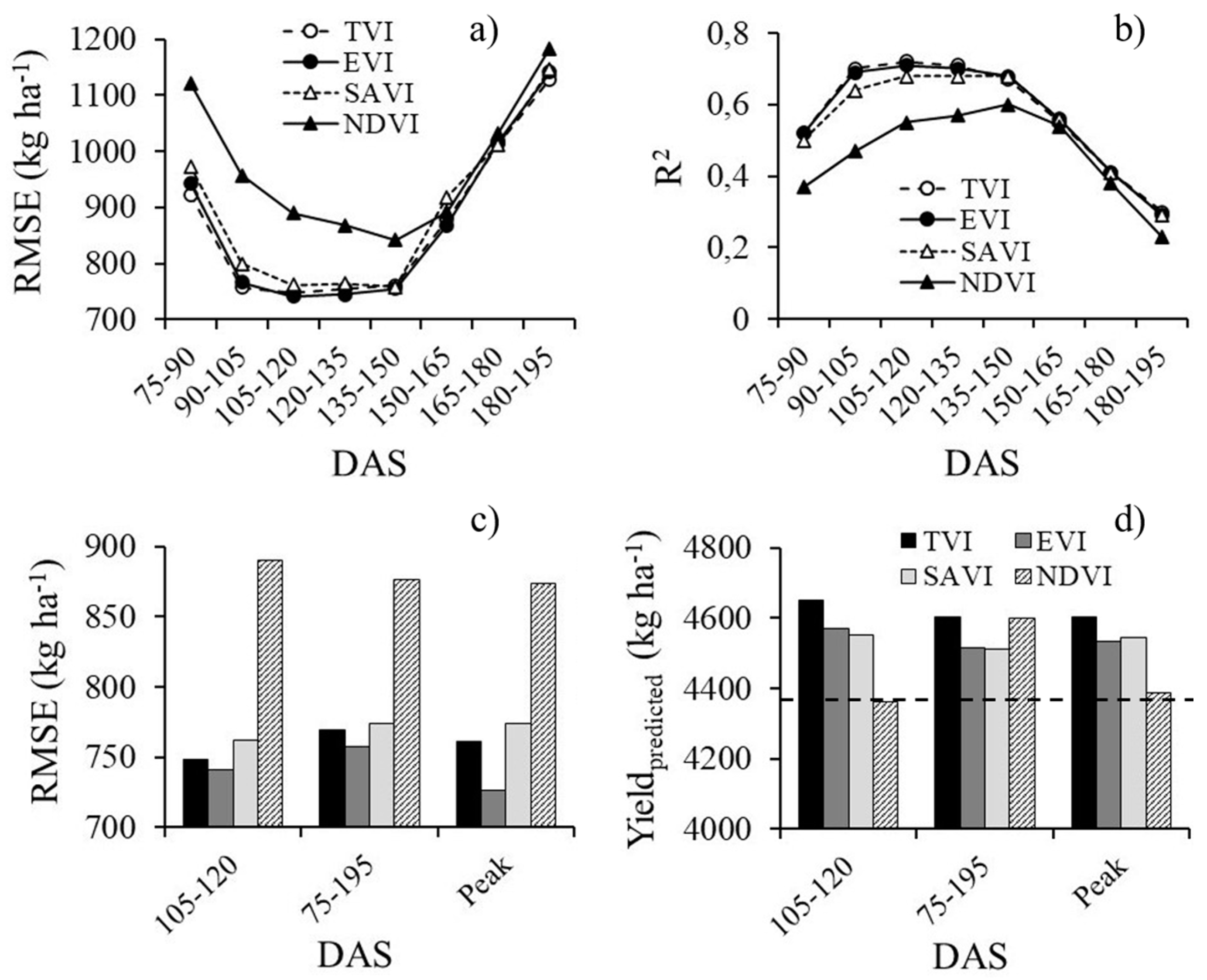
Table 2.
Vegetation indices used in this study.
| Vegetation Indices | Formulation | Reference |
|---|---|---|
| Green Index (GI) | GI = G/R | [44] |
| Ratio Vegetation Index (RVI) | RVI = NIR/R | [45] |
| Chlorophyll Vegetation Index (CVI) | CVI = (NIR*R)/G2 | [46] |
| Soil-Adjusted Vegetation Index (SAVI) | SAVI = 1.5*(NIR-R)/(0.5*NIR+R) | [47] |
| Chlorophyll index - green (CIG) | CIG = (NIR/G)-1 | [44] |
| Triangular Chlorophyll Absorption Ratio Index (TVI) | TVI = 60*NIR-G-100*(R-G) | [48] |
| Green NDVI (GNDVI) | GNDVI = (NIR-G)/(NIR+G) | [49] |
| Enhanced Vegetation Index (EVI) | EVI = 2.5*(NIR-R)/(1+NIR+6*R-7.5*B) | [50] |
| Normalized Differential Vegetation Index (NDVI) | NDVI = (NIR-R)/(NIR+R) | [51] |
| G: Green, R: Red, NIR: Near Infrared, B: Blue |
Table 3.
Linear regression models for predicting cotton yield from averaged 15-days TVI, EVI, SAVI and NDVI vegetation indices, averaged 75-195 DAS and peak (maximum value in the time-series), using the training dataset.
Table 3.
Linear regression models for predicting cotton yield from averaged 15-days TVI, EVI, SAVI and NDVI vegetation indices, averaged 75-195 DAS and peak (maximum value in the time-series), using the training dataset.
| DAS | Linear Model (TVI) | r2 | RMSE | DAS | Linear Model (EVI) | r2 | RMSE | |
|---|---|---|---|---|---|---|---|---|
| 75-90 | Y = 111.96 TVI + 794.22 | 0.31 | 1088 | 75-90 | Y = 5133.1 EVI + 315.9 | 0.28 | 1119 | |
| 90-105 | Y = 139.78 TVI - 90.918 | 0.47 | 953 | 90-105 | Y = 6863.1 EVI - 1066.8 | 0.46 | 966 | |
| 105-120 | Y = 152.11 TVI - 269.52 | 0.58 | 856 | 105-120 | Y = 7316.1 EVI - 1249.5 | 0.55 | 879 | |
| 120-135 | Y = 152.87TVI + 166.22 | 0.67 | 752 | 120-135 | Y = 7013.0 EVI - 608.5 | 0.65 | 778 | |
| 135-150 | Y = 148.0 TVI + 878.89 | 0.69 | 735 | 135-150 | Y = 6484.9 EVI + 292.1 | 0.68 | 778 | |
| 150-165 | Y = 147.88 TVI + 1553.7 | 0.64 | 783 | 150-165 | Y = 6170.2 EVI + 1127.9 | 0.65 | 776 | |
| 165-180 | Y = 162.65 TVI + 1957.8 | 0.59 | 843 | 165-180 | Y = 6456.5 EVI + 1636.5 | 0.59 | 842 | |
| 180-195 | Y = 195.06 TVI + 2130.5 | 0.49 | 941 | 180-195 | Y = 7602.2 EVI + 1801.6 | 0.48 | 947 | |
| 75-195 | Y = 196.28 TVI - 189.77 | 0.72 | 690 | 75-195 | Y = 8891.9 EVI - 1026.2 | 0.73 | 688 | |
| Peak | Y = 150.52 TVI - 634.87 | 0.53 | 900 | Peak | Y = 7813.9 EVI - 1996.1 | 0.53 | 901 | |
| DAS | Linear Model (SAVI) | r2 | RMSE | DAS | Linear Model (NDVI) | r2 | RMSE | |
| 75-90 | Y = 6804.1 SAVI - 543.3 | 0.25 | 1140 | 75-90 | Y = 6111.6 NDVI - 1057.4 | 0.12 | 1232 | |
| 90-105 | Y = 9495.4 SAVI - 2479.4 | 0.45 | 977 | 90-105 | Y = 11059 NDVI - 5334.6 | 0.31 | 1089 | |
| 105-120 | Y = 10008 SAVI - 2696 | 0.55 | 1132 | 105-120 | Y = 11093 NDVI - 5287.1 | 0.35 | 1058 | |
| 120-135 | Y = 9164.3 SAVI - 1712.5 | 0.64 | 784 | 120-135 | Y = 9500.8 NDVI - 3674.2 | 0.46 | 966 | |
| 135-150 | Y = 7937.6 SAVI - 415.88 | 0.67 | 753 | 135-150 | Y = 7473.6 NDVI - 1618 | 0.55 | 884 | |
| 150-165 | Y = 7729.7 SAVI + 624.53 | 0.66 | 809 | 150-165 | Y = 6243.6 NDVI - 80.36 | 0.61 | 816 | |
| 165-180 | Y = 7244.4 SAVI + 1251.7 | 0.59 | 840 | 165-180 | Y = 5550.8 NDVI + 1002 | 0.57 | 861 | |
| 180-195 | Y = 8316.9 SAVI + 1422.3 | 0.47 | 952 | 180-195 | Y = 5922.8 NDVI + 1386.4 | 0.46 | 970 | |
| 75-195 | Y = 11152 SAVI - 2066.5 | 0.73 | 688 | 75-195 | Y = 11230 NDVI + 4003.9 | 0.67 | 752 | |
| Peak | Y = 11045 SAVI - 3770 | 0.51 | 919 | Peak | Y = 15470 SAVI – 9331.6 | 0.39 | 1029 | |
| Y: seed cotton yield (kg ha-1); Peak: maximum value of the VI in the time-series | ||||||||
Disclaimer/Publisher’s Note: The statements, opinions and data contained in all publications are solely those of the individual author(s) and contributor(s) and not of MDPI and/or the editor(s). MDPI and/or the editor(s) disclaim responsibility for any injury to people or property resulting from any ideas, methods, instructions or products referred to in the content. |
© 2024 by the authors. Licensee MDPI, Basel, Switzerland. This article is an open access article distributed under the terms and conditions of the Creative Commons Attribution (CC BY) license (http://creativecommons.org/licenses/by/4.0/).
Copyright: This open access article is published under a Creative Commons CC BY 4.0 license, which permit the free download, distribution, and reuse, provided that the author and preprint are cited in any reuse.


