Analysing the Dynamics of Housing Price-Vacancy Relationship in the Hong Kong Housing Markets

1. Introduction

In the study of housing markets, understanding the determinants of housing prices is of paramount importance for policymakers, investors, and researchers alike. Traditionally, many studies have approached this issue by considering housing demand and supply as separate entities, estimating their effects on prices independently. However, this approach overlooks the intricate interplay between these factors and may yield inconsistent or unreliable results. For example, common proxies for demand include income levels, population growth, and interest rates. These variables provide insights into the purchasing power of potential homebuyers. The impact of the variables however, does very much depend on the inventory or number of vacant units. Similarly, indicators such as housing units-constructed, building permits or land availability are considered as proxies for housing supply. But the developers’ decisions on new developments are shaped by the level of inventory within the market.

It is understandable that treating demand and supply factors as separate entities is a practical solution to maintain model simplicity and estimation viability. However, some previous studies using separate demand-supply variables have found unexpectedly contradictory effects of supply, resulting in misinterpretations of the true drivers of housing price fluctuations.

To address these limitations, this study proposes a novel approach by utilising number of vacant units as a proxy for the net effect of supply and demand interactions on housing prices. By incorporating the number of vacant units as a determinant of housing prices, this study aims to analyse the net impact of the interplaying dynamics between housing supply and demand on housing prices. Specifically, the study hypothesises that changes in the number of vacant units will reflect the equilibrium between housing supply and demand, thus exerting a significant influence on housing prices.

It is well recognised that frequent housing vacancy data is often hardly available. Vacancy data is usually collected once every five years during the census, and accuracy of the data is hard to ascertain. This may explain why vacancy rates are not commonly used in studies of housing prices determinants. This study uses the annual data series of the numbers of vacant units of five different classes of housing in Hong Kong to examine the validity of the proposed hypothesis.

The preliminary findings suggest that changes of the number of vacant units impose a negative effect on changes of real housing prices, aligning with theoretical predictions. This underscores the importance of considering vacancy as a crucial determinant of housing prices, as vacancy encapsulates the outcome of the intricate interplay between the housing supply and demand dynamics. Through this innovative approach, the study aims to provide a more comprehensive understanding of the determinants of housing prices and contribute to more robust policymaking and investment strategies in the housing sector.

The paper is organised as follows: Section 2 is a literature review on existing studies of the determinants of housing prices and vacancy rates. Section 3 outlines the research materials and methods used. Section 4 reports the results of the empirical tests. Section 5 discusses the findings and implications. Section 6 concludes.

2. Literature Review

Supply-side Determinants of Housing Prices

The broad and diverse nature of residential housing markets means that there are various demand and supply side factors that interact to achieve an equilibrium and result in market housing prices (Xu and Tang, 2014). Sirmans et al. (2006), however, found the existing literature failed to reach a common consensus on the effect of different determinants on housing prices through hedonic pricing models. It implies that the outcomes of the studies can vary greatly depending on the model specifications. This variation can challenge the robustness of the findings.

The results of housing supply determinants are particularly confusing. There have been studies finding that housing supply is positively associated with housing prices which contradicts the prediction of the Law of Supply. The results are posited to support that housing supply change is determined by housing price change, instead of its determinant. For example, both Glindro et al. (2007) and Belke & Keil (2017) found a positive and significant association between land or housing supply and housing prices. Glindro et al. (2007: 186) studied determinants of house prices in nine Asia-Pacific economies. They concluded that “the coefficient of the land supply index is positive, which contradicts the theoretical prediction that increases in land supply have a dampening effect on house prices.” They tried to explain the contradictory results by contending that “higher house prices provide an incentive for developers to build up new residential property projects.” Similarly, Belke & Keil (2017: 14) analysed a panel dataset of nearly 100 German cities, with both supply-side and demand-side factors. They found that, among others, “The positive relation between construction activity and real estate prices could reflect a supply side reaction of increasing construction in cities with strong demand.” Many other studies found no significant results of housing supply. For example, Taghizadeh-Hesary, Yoshino & Chiu (2019: 18) of ADBI analysed a time series dataset in 1999–2018 of macroeconomic variables and housing prices in Hong Kong, and they also found that, among others, “housing supply has never been statistically significant; housing supply is not responsible for or affected by, or does it respond to price changes”.

In contrast, there are studies that claimed to find a negative association between housing supply and prices. Geng (2018), for instance, studied determinants of house prices of 20 advanced economies by a cross-country panel model and found a negative effect of housing supply on house prices. Yet, the proxy of supply is housing stock per capita. Similarly, Dröes & van de Minne (2017) also found a negative relationship between housing supply and prices by using the total number of housing units in Amsterdam as the proxy of supply.

Demand-side Determinants of Housing Prices

Studies on demand-side determinants of housing prices do have consistent results, especially on investment demand proxies, such as interest rates and GDP. Égert & Mihaljek (2007) studied the determinants of house prices in eight transition economies of Europe and 19 OECD countries and found that real interest rates and GDP per capita are two strong demand-side price determinant. These two demand-side price determinants are echoed through other studies that often use interest rates, GDP or a subsidiary of GDP as a means to understand the demand side pressures impacting upon house prices. (Glindro et al., 2007; Xu & Tang, 2014; Dröes & van de Minne, 2017; Taghizadeh-Hesary, Yoshino & Chiu, 2019; Yiu, 2021).

Studies on Housing Vacancy

Instead of including separate proxies of housing demand and supply, Égert & Mihaljek (2007: 3) contended that “both the supply and demand for housing interact to determine an equilibrium level for real house prices”. But they did not identify any proxies of the interaction results.

Theoretically, Wheaton (1990: 1290) developed one of the first housing vacancy model which “suggests that small changes in supply or demand, as they alter vacancy, can have very profound impacts on market prices.” Understanding the intricate relationship between housing prices and vacancy rates is crucial for policymakers, real estate investors, and analysts alike. However, as reviewed above, very few studies on house prices determinants would include vacancy as a determinant, probably due to the unavailability of vacancy time series. Previous studies on housing vacancy often relied on cross-sectional data, such as Lerbs & Teske (2016), which are hard to control all spatial differences and could not capture the temporal dynamics adequately. Furthermore, such cross-sectional studies are susceptible to endogeneity and omission biases, casting doubts on the reliability of their findings. Thus, this study attempts to analyse the temporal effects of vacancy changes on housing price changes, ceterus paribus.

3. Materials and Methods

3.1. Data

The dataset for this study is collected from Rating and Valuation Department (RVD, 2024) which provides yearly vacancy rates and housing prices for five distinct classes of housing units, categorised by their floor areas, in Hong Kong. Other demographic and macroeconomic data are collected from Census and Statistics Department (C&SD, 2024). Both time series and panel analysis methods are employed to investigate the relationship between housing vacancies and prices over time, controlling for various housing sizes and temporal factors.

Housing data in Hong Kong are reported in five classes, based on the saleable area of housing units, viz. (a) Class A – less than 40 sq. m.; (b) Class B – from 40 to 69.9 sq. m.; (c) Class C – from 70 to 99.9 sq. m.; (d) Class D – from 100 to 159.9 sq. m.; and (e) Class E – from 160 sq. m. and above. Figure 1 shows the vacancies of the five classes of housing in Hong Kong from 1997 to 2022. Classes A and B are the dominant sizes as they account for 80% (A: 32% and B: 48%) of total housing stock (1,256,772) in 2022. Classes C, D and E account for 12%, 6%, and 2% respectively (RVD, 2024).

Figure 1. Vacancies of the five classes of housing in Hong Kong from 1997 to 2022. Source: RVD (2024). Legends: Classes of housing are categorised based on the saleable area of housing units, viz. (a) Class A – less than 40 sq. m.; (b) Class B – from 40 to 69.9 sq. m.; (c) Class C – from 70 to 99.9 sq. m.; (d) Class D – from 100 to 159.9 sq. m.; and (e) Class E – from 160 sq. m. and above.

Figure 1. Vacancies of the five classes of housing in Hong Kong from 1997 to 2022. Source: RVD (2024). Legends: Classes of housing are categorised based on the saleable area of housing units, viz. (a) Class A – less than 40 sq. m.; (b) Class B – from 40 to 69.9 sq. m.; (c) Class C – from 70 to 99.9 sq. m.; (d) Class D – from 100 to 159.9 sq. m.; and (e) Class E – from 160 sq. m. and above.

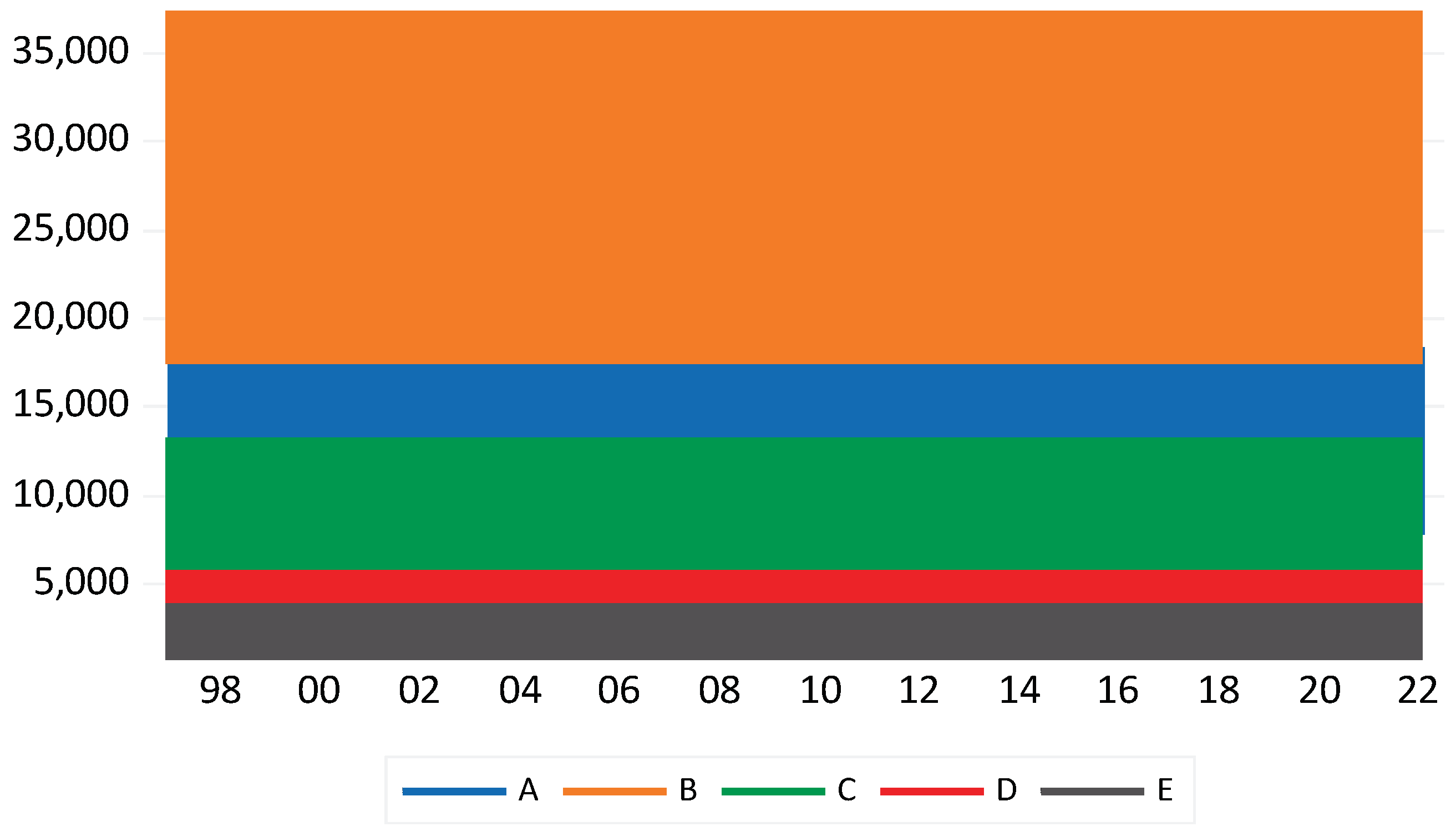
The vacancy of small-sized residential units (Class A) shows a recent increasing trend, while the vacancies of medium-sized residential units (Classes B and C) rose to the peak in around 2002-2003 and then fell afterwards. The vacancies of large units have remained relatively steady.

Similarly, the yearly series of housing completion rate of each housing class is collected from the RVD (2024). Demand proxies, including population, real GDP, interest rate, are common to all housing classes. Table 1 shows the descriptive statistics of the variables, and Table 2 shows their stationarities by the Levin, Lin & Chu test and the Im, Peasaran and Shin test. They show that all series are stationary in their first differences.

Table 1. Descriptive Statistics of Variables, 1997–2022. Sources: RVD (2024) & C&SD (2024).

Variable	Class	Mean	Standard Deviation	Minimum	Maximum
Natural logarithm of the real housing price index of class i in year t, ln(RHPt)	A	0.75	0.53	-0.10	1.46
	B	0.70	0.46	-0.08	1.32
	C	0.73	0.40	-0.01	1.24
	D	0.77	0.37	0.06	1.20
	E	0.83	0.36	0.15	1.21
	Combined	0.73	0.47	-0.07	1.36
Natural logarithm of the number of vacant housing units of class i in year t, ln(VACt)	A	9.34	0.26	9.00	9.80
	B	10.11	0.24	9.79	10.53
	C	8.98	0.24	8.47	9.49
	D	8.40	0.22	7.74	8.64
	E	7.80	0.30	6.99	8.25
	Combined	10.85	0.17	10.49	11.21
Natural logarithm of the number of class i housing units completed in year t, ln(COMt)	A	7.81	0.90	5.92	9.20
	B	9.06	0.55	8.01	9.95
	C	7.87	0.48	7.10	8.89
	D	6.92	0.51	5.52	7.66
	E	5.98	0.44	4.80	6.79
	Combined	9.70	0.44	8.88	10.47
Natural logarithm of the population in year t, ln(POPt)	-	15.77	0.04	15.69	15.83
Natural logarithm of real gross domestic products in year t, ln(RGDPt)	-	10.05	0.17	9.74	10.29
Interbank 3-month offer interest rate of Hong Kong in year t, IRt	-	0.86	3.94	-4.87	10.11
Period	1997–2022
Number of Observations	130 Obs (26 periods × 5 classes)

Table 1. Descriptive Statistics of Variables, 1997–2022. Sources: RVD (2024) & C&SD (2024).

Variable	Class	Mean	Standard Deviation	Minimum	Maximum
Natural logarithm of the real housing price index of class i in year t, ln(RHPt)	A	0.75	0.53	-0.10	1.46
	B	0.70	0.46	-0.08	1.32
	C	0.73	0.40	-0.01	1.24
	D	0.77	0.37	0.06	1.20
	E	0.83	0.36	0.15	1.21
	Combined	0.73	0.47	-0.07	1.36
Natural logarithm of the number of vacant housing units of class i in year t, ln(VACt)	A	9.34	0.26	9.00	9.80
	B	10.11	0.24	9.79	10.53
	C	8.98	0.24	8.47	9.49
	D	8.40	0.22	7.74	8.64
	E	7.80	0.30	6.99	8.25
	Combined	10.85	0.17	10.49	11.21
Natural logarithm of the number of class i housing units completed in year t, ln(COMt)	A	7.81	0.90	5.92	9.20
	B	9.06	0.55	8.01	9.95
	C	7.87	0.48	7.10	8.89
	D	6.92	0.51	5.52	7.66
	E	5.98	0.44	4.80	6.79
	Combined	9.70	0.44	8.88	10.47
Natural logarithm of the population in year t, ln(POPt)	-	15.77	0.04	15.69	15.83
Natural logarithm of real gross domestic products in year t, ln(RGDPt)	-	10.05	0.17	9.74	10.29
Interbank 3-month offer interest rate of Hong Kong in year t, IRt	-	0.86	3.94	-4.87	10.11
Period	1997–2022
Number of Observations	130 Obs (26 periods × 5 classes)

Table 2. Unit Root Tests of Variables, 1997–2022.

Variable	Level		First-Difference
Time Series	ADF	PP	ADF	PP
ln(RHPt)	-0.30	-0.35	-4.56 ***	-4.56 ***
ln(VACt)	-2.49	-2.51	-5.36 ***	-5.36 ***
ln(COMt)	-1.28	-1.93	-7.87 ***	-7.78 ***
ln(POPt)	-1.64	-1.57	-5.73 ***	-6.10 ***
ln(RGDPt)	-1.20	-1.28	-5.16 ***	-5.27 ***
IRt	-2.79 *	-1.69	-	-
Panel	Levin, Lin & Chu t*	Im, Peasaran and Shin W-stat	Levin, Lin & Chu t*	Im, Peasaran and Shin W-stat
ln(RHPt)	0.87	2.11	-6.03 ***	−5.31 ***
ln(VACt)	-1.90 **	-1.84 **	-4.84 ***	-7.39 ***
ln(COMt)	-1.41 *	-2.68 ***	-9.14 ***	-10.00 ***
ln(POPt)	-1.90 **	1.02	-8.60 ***	-9.70 ***
ln(RGDPt)	-1.85 **	0.82	-8.58 ***	−8.03 ***
IRt	-3.53 ***	-3.06 ***	-	-

Notes: figures are statistics, ***, ** and * represent p-value ≤ 0.01, 0.05 and 0.10, respectively. The panel unit root tests used Newey-West automatic bandwidth selection and Quadratic Spectral kernel, with automatic lag length selection based on SIC: 0 to 5, and automatic selection of maximum lags.

Table 2. Unit Root Tests of Variables, 1997–2022.

Variable	Level		First-Difference
Time Series	ADF	PP	ADF	PP
ln(RHPt)	-0.30	-0.35	-4.56 ***	-4.56 ***
ln(VACt)	-2.49	-2.51	-5.36 ***	-5.36 ***
ln(COMt)	-1.28	-1.93	-7.87 ***	-7.78 ***
ln(POPt)	-1.64	-1.57	-5.73 ***	-6.10 ***
ln(RGDPt)	-1.20	-1.28	-5.16 ***	-5.27 ***
IRt	-2.79 *	-1.69	-	-
Panel	Levin, Lin & Chu t*	Im, Peasaran and Shin W-stat	Levin, Lin & Chu t*	Im, Peasaran and Shin W-stat
ln(RHPt)	0.87	2.11	-6.03 ***	−5.31 ***
ln(VACt)	-1.90 **	-1.84 **	-4.84 ***	-7.39 ***
ln(COMt)	-1.41 *	-2.68 ***	-9.14 ***	-10.00 ***
ln(POPt)	-1.90 **	1.02	-8.60 ***	-9.70 ***
ln(RGDPt)	-1.85 **	0.82	-8.58 ***	−8.03 ***
IRt	-3.53 ***	-3.06 ***	-	-

Notes: figures are statistics, ***, ** and * represent p-value ≤ 0.01, 0.05 and 0.10, respectively. The panel unit root tests used Newey-West automatic bandwidth selection and Quadratic Spectral kernel, with automatic lag length selection based on SIC: 0 to 5, and automatic selection of maximum lags.

3.2. Research Design

A time series regression model and a five-class panel regression model (Equation (1)) use the traditional approach of separated variables for housing demand and supply are conducted as the baseline models. Population, real GDP and interest rate are incorporated to estimate demand effects, whereas housing completion is taken as the proxy of housing supply. Corresponding models (Equation (2)) uses the number of vacant housing units as an indicator of net demand which is then exploited to test the vacancy hypothesis. Interest rate variable is retained to estimate investment demand, which is less affected by vacancy rate.

$$dln\left({RHP}_{it}\right)={c_1+{\alpha }_i+\beta }_1{dln(POP}_t)+{\beta }_2{dln(RGDP}_t)+{\beta }_3{(IR}_t)+{\beta }_4{dln(COM}_{it})+\gamma dln\left({RHP}_{i,t-1}\right)+{\epsilon }_{it}$$

(1)

$$dln\left({RHP}_{it}\right)={c_1+\alpha }_i+{\beta }_3{(IR}_t)+{\beta }_5{dln(VAC}_{it})+\gamma dln\left({RHP}_{i,t-1}\right)+{\epsilon }_{it}$$

(2)

where RHP_it, POP_t, RGDP_t, IR_t, COM_it, and VAC_it, are real house price indices, population, real gross domestic products, interest rates, number of housing units completed and number of vacant units (of class i in panel models or of the combined series in time series models) at time t. ${\alpha }_i$ control cross-class fixed effects in the panel model, $\gamma dln\left({RHP}_{i,t-1}\right)$ caters for the autoregressive effect of house price changes in a one-year lag.${\beta }_1,{\beta }_2,{\beta }_3,{\beta }_4,{\beta }_5,\gamma$are coefficients to be estimated. ${\epsilon }_{it}$ is the error term.

In the time series models, the combined series of real house price index, vacancies and completions are directly provided by RVD (2024). The Autoregressive Moving Averages (ARMA) model is applied to analyse the time series variables, using the Broyden-Fletcher-Goldfarb-Shanno (BFGS) method to estimate the coefficients of the ARMA models. The BFGS algorithm is a numerical optimisation technique commonly used to maximise the likelihood function in Maximum Likelihood Estimation (MLE).

The panel models control class-specific factors by a cross-sectional fixed effect such as the policy changes in stamp duty and mortgage lending. The Panel Error Components Generalised Least Squares (EGLS) method. Since we found a significant cross-section dependence (correlation) between price changes of different housing classes, as shown in the Breusch-Pagan Lagrange Multiplier test (statistic=239.5, df=10, p=0.000), a cross-section seemingly unrelated regression (SUR) is used as generalised least squares (GLS) weights in the panel models to estimate the parameters. Furthermore, a Panel-Corrected Standard Errors (PCSE) technique is applied to correct the standard errors and covariance matrix of the estimated coefficients to address heteroscedasticity issue.

4. Results

Utilising both time series and panel regression models, Models 1a and 1b in Table 3 show the results of the temporal impacts of separate demand and supply factors as well as net demand factor proxied by changes of number of vacant units on housing price changes, with housing size effects fixed in the panel analysis. In the baseline models, the results show a negative effect of population size change in both models, which contradicts theoretical prediction. Also, a 1% increase in real GDP is found to have a positive (about 2% increase) and significant impact on housing prices in both models. Interest rate effect is negative as expected, however, it is insignificant in the time series model, and marginally significant in the panel model. Housing supply proxied by changes of housing completion is found to impose a negative effect on housing prices, but statistically insignificant in both models. The results of parameters in contradictory sign and of weak significance in most of the demand and supply variables agree with that of many previous studies and indicate a potential model misspecification.

However, housing supply is commonly agreed to be inelastic and takes time to complete. Model 2b of Table 3 shows a stronger and significant negative effect of housing supply if a 3-year lead is considered. Yet, how long being the lagging period is an empirical question and can vary over time. Due to the lagging nature of supply responses, it supports the use of vacancy data to estimate the net demand effect, as it represents the actual dynamics of demand and supply at any point of time.

Models 3a and 3b of Table 3, showed a consistently negative and significant effect of vacancy on housing prices, no matter in time series or in panel models. These findings suggest that housing vacancy is a price determinant, reflecting the net result of a dynamic interplay between housing demand and supply. The panel analysis allows us to disentangle the temporal trends from housing size factors, providing a more accurate depiction of the housing vacancy price relationship. The results highlight the importance of considering both temporal and spatial dimensions in understanding the complex dynamics of the real estate market.

Models 4a and 4b of Table 3 further divide housing demand into investment demand and accommodation demand, vacancy is assumed to be the net demand of accommodation and interest rate is considered as a proxy of investment demand which is independent of accommodation demand. The effect of vacancies on housing prices is quite similar to Models 3a and 3b. The interest rate effect is found, as expected, to be negative and significant and the magnitude is about the same as in Models 2a and 2b, supporting the use of vacancy variable as a proxy of net accommodation demand.

Table 3. Results of the time series and panel regression models on the determinants of house price change.

Dependent Variable	dln(RHPt)				dln(RHPit)
Variables	Time Series Model 1a	Time Series Model 2a	Time Series Model 3a	Time Series Model 4a	Panel Model 1b	Panel Model 2b	Panel Model 2b	Panel Model 3b
dln(POPt)	-3.272 (-0.52)	-14.609 (-1.61)	-	-	-6.999 (-1.91) *	-16.134 (-3.56) ***	-	-
dln(COMit)	-0.004 (-0.05)	-	-	-	-0.002 (-0.66)	-	-	-
dln(COMit+3)	-	-0.047 (-0.73)	-	-	-	-0.008 (-2.67) ***	-	-
dln(RGDPt)	2.131 (3.67) **	2.907 (6.58) ***	-	-	2.241 (5.47) ***	3.033 (7.94) ***	-	-
dln(VACit)	-	-	-0.795 (-3.18) **	-0.630 (-2.15) **	-	-	-0.024 (-2.89) ***	-0.022 (-3.04) ***
IRt	-0.018 (-1.45)	-0.017 (-0.94)	-	-0.013 (-1.04)	-0.014 (-1.67) *	-0.025 (-2.40) **	-	-0.026 (-2.53) **
AR(1)	0.187 (0.78)	0.598 (1.96) *	-0.505 (-2.88) ***	-0.538 (-2.23) **	0.208 (2.40) **	0.435 (4.80) ***	0.185 (1.58)	0.121 (1.29)
Constant	0.056 (1.21)	0.129 (1.57)	0.041 (2.29) **	-1.216 (-1.01)	0.059 (1.86) *	0.124 (2.82) ***	0.026 (0.74)	0.086 (2.56) **
Fixed Effect	NA				Yes (on housing classes)
Model	ARMA Maximum Likelihood (BFGS)				Panel EGLS (Cross-section SUR) with cross-section weights (PCSE) std errors & covariance
Sample (year)	1997-2022
No. of Obs.	26	23	26	26	130 (26x5)	115 (23x5)	130 (26x5)	130 (26x5)
Adj. R-Squared	0.34	0.50	0.16	0.22	0.20	0.43	0.04	0.11

Notes: Figures in parenthesis are t-statistics, ***, ** and * represent p-value ≤ 0.01, 0.05 and 0.10, respectively.

Table 3. Results of the time series and panel regression models on the determinants of house price change.

Dependent Variable	dln(RHPt)				dln(RHPit)
Variables	Time Series Model 1a	Time Series Model 2a	Time Series Model 3a	Time Series Model 4a	Panel Model 1b	Panel Model 2b	Panel Model 2b	Panel Model 3b
dln(POPt)	-3.272 (-0.52)	-14.609 (-1.61)	-	-	-6.999 (-1.91) *	-16.134 (-3.56) ***	-	-
dln(COMit)	-0.004 (-0.05)	-	-	-	-0.002 (-0.66)	-	-	-
dln(COMit+3)	-	-0.047 (-0.73)	-	-	-	-0.008 (-2.67) ***	-	-
dln(RGDPt)	2.131 (3.67) **	2.907 (6.58) ***	-	-	2.241 (5.47) ***	3.033 (7.94) ***	-	-
dln(VACit)	-	-	-0.795 (-3.18) **	-0.630 (-2.15) **	-	-	-0.024 (-2.89) ***	-0.022 (-3.04) ***
IRt	-0.018 (-1.45)	-0.017 (-0.94)	-	-0.013 (-1.04)	-0.014 (-1.67) *	-0.025 (-2.40) **	-	-0.026 (-2.53) **
AR(1)	0.187 (0.78)	0.598 (1.96) *	-0.505 (-2.88) ***	-0.538 (-2.23) **	0.208 (2.40) **	0.435 (4.80) ***	0.185 (1.58)	0.121 (1.29)
Constant	0.056 (1.21)	0.129 (1.57)	0.041 (2.29) **	-1.216 (-1.01)	0.059 (1.86) *	0.124 (2.82) ***	0.026 (0.74)	0.086 (2.56) **
Fixed Effect	NA				Yes (on housing classes)
Model	ARMA Maximum Likelihood (BFGS)				Panel EGLS (Cross-section SUR) with cross-section weights (PCSE) std errors & covariance
Sample (year)	1997-2022
No. of Obs.	26	23	26	26	130 (26x5)	115 (23x5)	130 (26x5)	130 (26x5)
Adj. R-Squared	0.34	0.50	0.16	0.22	0.20	0.43	0.04	0.11

Notes: Figures in parenthesis are t-statistics, ***, ** and * represent p-value ≤ 0.01, 0.05 and 0.10, respectively.

5. Discussion

The use of separate variables to estimate housing demand and supply effects on prices can be shown to be biased by a simple thinking experiment. Imagine whenever housing demand increases/decreases, housing supply increases/decreases at the same time but with 50% quantity. In other words, net demand will be positive/negative when demand increases/decreases. However, in a traditional regression model with separate proxies for demand and supply, since both of them always move in the same direction as in this case, their effects on prices would be of the same sign, which is contradictory to the Laws of Supply and Demand. It is because they are assumed to be independent in the regression model, but in reality, they are inextricably intertwined. It can be rectified by using net demand, that is the resultant of the interplay of housing demand and supply, which reflect the actual lagging nature and inelasticity of housing supply of the housing markets.

The availability and accuracy of vacancy data are crucial for understanding and predicting housing market dynamics, including the determinants of housing prices. However, traditional methods of collecting vacancy data, such as those conducted during the census once every five years, present challenges due to their infrequency and varying definitions across different jurisdictions. Fortunately, advancements in technology, particularly the digitalisation of utility meters, offer a promising solution to these challenges. By leveraging the data from digital electricity and water meters, cities can standardise the definition of vacant homes and collect meaningful vacancy data for housing price analysis.

In recent years, the digitalisation of utility meters, particularly electricity and water meters, has transformed the way utility consumption data is collected and analysed (Razavo, et al., 2019; Newing et al., 2023). Digital meters provide real-time monitoring of energy and water usage in homes, offering a wealth of data that can be leveraged to identify vacant properties. By setting a threshold for electricity and/or water consumption below which a property is considered vacant, cities can establish a standardised definition of vacant homes, overcoming the inconsistencies associated with traditional vacancy data collection methods.

Leveraging digital utility meters for vacancy data collection offers several advantages. First and foremost, it enables real-time monitoring of vacancy rates, allowing policymakers and researchers to track changes in housing market dynamics more accurately and promptly. Second, by standardising the definition of vacant homes based on utility consumption thresholds, cities can ensure consistency and comparability in vacancy data across different jurisdictions. This enhances the reliability and usefulness of vacancy data for housing price analysis and policymaking. Additionally, the use of digital utility meters reduces the burden and cost associated with traditional vacancy surveys, as data collection can be automated and conducted remotely.

The availability of standardised vacancy data collected through digital utility meters opens up new possibilities for analysing the determinants of housing prices. Researchers can incorporate vacancy data as an important explanatory variable in econometric models of housing prices, providing insights into the relationship between housing supply and demand dynamics. By leveraging real-time vacancy data, policymakers can develop more effective strategies to address housing market imbalances and promote housing affordability. Furthermore, the standardised nature of vacancy data collected through digital utility meters facilitates cross-city and cross-country comparisons, enabling researchers to identify trends and best practices in housing market regulation and policy implementation.

6. Conclusions

This is probably the first time series and panel analysis study of housing vacancies effect on prices. One of the major implications of the study is on identifying net demand determinants of housing prices. Traditionally, studies on price determinants treated housing supply and demand as separate independent variables in regression models, overlooking their interdependence. However, market prices emerge from the intricate interplay between supply and demand forces. Meaning they could not be independent. Also, finding appropriate proxies of housing demand can be challenging, as it is an economic construct rather than a directly observable information. Many previous studies considered population size and gross domestic products as demand proxies, without considering housing supply responses. Even if the studies incorporate proxies of supply, insignificant results or even contradictory results are often estimated. This study challenges the conventional approach by considering housing vacancy changes as outcomes of the interactions between supply and demand, i.e. net demand of accommodation. It can reflect accurately the dynamics of demand and supply of accommodation. A higher vacancy signifies an increased number of housing units that are neither utilised for owner-occupation nor rented out. The underlying reasons for such vacancies are diverse, including potential over-supply of building units in the market or an economic downturn leading to diminished accommodation demand for housing, or both. Conversely, a decrease in the vacancy may indicate a surge in net housing demand for accommodation, thereby exerting upward pressure on property prices.

By leveraging a panel analysis on a unique dataset from Hong Kong, this study advances our understanding of the housing vacancy - price relationship. The approach allows for a more accurate assessment of temporal trends, addressing the limitations of previous cross-sectional studies. The findings contribute to both academic research and practical applications in the real estate market, emphasising the importance of considering temporal interactions between housing demand and supply attributes in housing market analyses.

The previous lack of use of the housing vacancy variable as a determinant of housing prices could have arguably occurred due to its data unavailability. Currently, vacancy data is surveyed once every census, and different countries define housing vacancy differently. Hence the digitalisation of utility meters presents a transformative opportunity to modernise vacancy data collection for housing price analysis. Utilising data gathered from digital electricity and water meters, establishing a standardised definition for vacant properties, and collecting real-time vacancy information can help to address the constraints posed by conventional vacancy surveys.

Researchers can incorporate vacancy data more frequently as an important explanatory variable in econometric models of housing prices, providing insights into the relationship between housing supply and demand dynamics. By leveraging real-time vacancy data, policymakers can develop more effective strategies to address housing market imbalances and promote housing affordability. Furthermore, the standardised nature of vacancy data collected through digital utility meters facilitates cross-city and cross-country comparisons, enabling researchers to identify trends and best practices in housing market regulation and policy implementation.

References

- Belke, A. & Keil, J. (2017). Fundamental determinants of real estate prices: A panel study of German regions, Ruhr Economic Papers, №731, ISBN 978–3–86788–851–6, RWI — Leibniz-Institut für Wirtschaftsforschung, Essen. [CrossRef]
- C&SD (2024). Statistics by subject. Census and Statistics Department, HKSAR Government. Available online: https://www.censtatd.gov.hk/en/page_8000.html. Accessed on 18 January 2024.
- Dröes, M.I. & van de Minne, A. (2017). Do the Determinants of House Prices Change over Time? Evidence from 200 Years of Transactions Data, American Economic Association. https://www.aeaweb.org/conference/2017/preliminary/paper/7NHnQiSz.
- Égert, B. & Mihaljek, D. (2007). Determinants of house prices in central and eastern Europe, BIS Working Papers no. 236, https://www.bis.org/publ/work236.pdf.
- Feng, Y. Examining the determinants of housing prices and the influence of the spatial–temporal interaction effect: The case of China during 2003–2016. Chinese Journal of Population, Resources and Environment 2020, 18, 59–67. [Google Scholar] [CrossRef]
- Geng, N. (2018). Fundamental Drivers of House Prices in Advanced Economies, IMF Working Paper, WP/18/164.
- Glindro, E.T.; Subhanij, T.; Szeto, J.; Zhu, H. Determinants of house prices in nine Asia-Pacific economies. In Research and Policy Analysis; Bank for International Settlements: Basel, Switzerland, 2007. [Google Scholar]
- Lerbs, O. and Teske, M. (2016). The House Price-Vacancy Curve, Discussion Paper No. 16-082, Centre for European Economic Research (ZEW). Available online at http://ftp.zew.de/pub/zew-docs/dp/dp16082.pdf. Retrieved on 18 January 2024.
- Newing, A.; Hibbert, O.; Van-Alwon, J.; Ellaway, S.; Smith, A. Smart water metering as a non-invasive tool to infer dwelling type and occupancy – Implications for the collection of neighbourhood-level housing and tourism statistics. Computers, Environment and Urban Systems 2023, 105, 102028. [Google Scholar] [CrossRef]
- Razavi, R.; Gharipour, A.; Fleury, M.; Akpan, I.J. Occupancy detection of residential buildings using smart meter data: A large-scale study. Energy and Buildings, 2019, 183, 195–208. [Google Scholar] [CrossRef]
- RVD (2024) Property Market Statistics, Publications. Rating and Valuation Department, HKSAR Government. Available online: https://www.rvd.gov.hk/en/publications/property_market_statistics.html. Accessed on 18 January 2024.
- Sirman, G. The Value of Housing Characteristics: A Meta Analysis. The Journal of Real Estate Finance and Economics 2006, 33, 215-240. Taghizadeh-Hesary, F., Yoshino, N. & Chiu, A. (2019). Internal and External Determinants of Housing Price Booms in Hong Kong, China, ADBI Working Paper Series, № 948, May. https://www.adb.org/sites/default/files/publication/503436/adbi-wp948.pdf.
- Wheaton, W.C. Vacancy, Search, and Prices in a Housing Market Matching Model. Journal of Political Economy 1990, 98, 1270–1292. [Google Scholar] [CrossRef]
- Xu, L. & Tang, B. On the Determinants of UK House Prices. International Journal of Economic Research 2014, 5, 57–64. [Google Scholar]
- Yiu, C.Y. Why House Prices Increase in the COVID-19 Recession: A Five-Country Empirical Study on the Real Interest Rate Hypothesis. Urban Science 2021, 5, 77. [Google Scholar] [CrossRef]
Disclaimer/Publisher’s Note: The statements, opinions and data contained in all publications are solely those of the individual author(s) and contributor(s) and not of MDPI and/or the editor(s). MDPI and/or the editor(s) disclaim responsibility for any injury to people or property resulting from any ideas, methods, instructions or products referred to in the content. |
© 2024 by the authors. Licensee MDPI, Basel, Switzerland. This article is an open access article distributed under the terms and conditions of the Creative Commons Attribution (CC BY) license (http://creativecommons.org/licenses/by/4.0/).
Copyright: This open access article is published under a Creative Commons CC BY 4.0 license, which permit the free download, distribution, and reuse, provided that the author and preprint are cited in any reuse.