Estimating Wastewater Dilution Using Chemical Markers and Incomplete Flow Measurements: Application to Normalisation of SARS-CoV-2 Measurements

We construct a Bayesian estimator for the dilution of a wastewater sample, and use it to estimate the prevalence of SARS-CoV-2 in Wales using data from the Wales Environmental Wastewater Analysis and Surveillance for Health project (WEWASH). In Wales wastewater is diluted by rainwater so an estimate of the level of dilution is required if we are to normalise sample measurements of disease markers such as SARS-CoV-2 RNA. We consider the situation where flow measurements are available, but will regularly be unreliable because of the action of combined sewer outflows, which divert wastewater away from treatment plants when the flow is excessive. However we also have proxies for the flow from various chemical markers, whose level per unit of population is fixed. The new estimator has multiple advantages compared to existing procedures: credible intervals for the estimates; optimal weighting of the chemical markers; systematic handling of missing and censored values; and model based smoothing without lags.

Keywords:

SARS-CoV-2

;

wastewater-based epidemiology

;

wastewater

;

dilution

;

flow normalisation

;

Bayesian

Subject:

Environmental and Earth Sciences - Water Science and Technology

This preprints belongs to the Collection

Preprints on COVID-19 and SARS-CoV-2

1. Introduction

Wastewater samples can be used to estimate the prevalence of disease in a community through the measurement of related biological markers, a process known as wastewater-based epidemiology (WBE). For example, in response to the COVID-19 pandemic wastewater monitoring programmes were introduced across the globe, measuring levels of SARS-CoV-2 (Naughton et al. [9], Perry et al. [11]). Biological markers of interest originate from sources such as faeces, urine and other bodily fluids that are flushed through the sewer system (Jones et al. [5]). Intuitively, the level of a disease marker sampled from wastewater should directly reflect disease prevalence in the community served by that sewer. However, biological markers can decay as they travel from their source (e.g. toilets) to the location where the wastewater sample is taken, and in addition wastewater networks are complex, and rarely receive inputs from just domestic sources. One of the most important inputs which can influence the effective measurement of disease prevalence in wastewater is extraneous water, which can enter the network via rainwater runoff or groundwater infiltration. Estimating the level of extraneous water is crucial because it is necessary to know the degree of dilution to be able to relate the level of a biological marker in the wastewater to the prevalence of the disease in the community.

Measuring wastewater flow at the sampling point—typically a wastewater treatment plant (WWTP)—is the most direct way of estimating the dilution of the sample, but this is not without its problems. Any diversion of wastewater between the source and the sampling point will confound the link between flow and dilution. That is, if our signal is diluted by a volume v per unit time, but a volume w per unit time of wastewater is being diverted before reaching the sampling point, then our observed flow of

v - w

no longer corresponds to the actual dilution. Wastewater can be lost by seepage or can spill into the natural environment through combined sewer overflows (CSOs). CSOs are active during times of high flow, when the capacity of the wastewater network has been reached, and prevent wastewater backing-up into properties (Perry et al. [10]). Wastewater can also be temporarily diverted to storage tanks. As biological markers will continue to decay or be lost while being stored, their levels per unit volume of wastewater will thus underestimate disease prevalence in the community.

On the other hand, chemical markers are on the whole less prone to decay than biological markers, and some are released in sewers at a relatively constant level per person. For example, the quantities of ammonia, orthophosphate and electrical conductivity in wastewater are proportional to the size of the contributing population, so their level per unit volume is proportional to the degree of dilution (Been et al. [1]; Langeveld et al. [7]; Sweetapple et al. [15]). Chemical markers thus offer an option to estimate the dilution of biological markers in wastewater (Wilde et al. [17]).

In this paper, we consider the problem of estimating wastewater dilution given noisy and sometimes unreliable flow measurements, with the aid of chemical markers. Flow measurements will be considered unreliable when wastewater has been diverted from the network by CSOs, or when the flow is so low that material can not be effectively transported through the network. The new dilution estimator we develop can then be used to convert the level of a biological marker in wastewater (for example SARS-CoV-2 gene copies per litre) to an estimate of the level of the biological marker per person. Here we apply this approach to counts of SARS-CoV-2 gene copies in wastewater across Wales (UK). Our approach is similar to that of Wilde et al. [17], but by using a Bayesian framework that explicitly models measurement errors we incorporate four improvements:

Credible intervals for estimates;
Optimal weighting of different chemical markers;
Systematic handling of missing and censored values, including observations below the limit of detection (LOD);
Model based smoothing without lags.

Additionally we make use of newly available data on combined sewer overflow (CSO) activity to judge when flow measurements are unreliable, allowing better use of available flow data.

Our estimator is applied to data collected as part of the Wales Environmental Wastewater Analysis and Surveillance for Health (WEWASH) project, a collaborative effort between the public sector (Welsh Government and Public Health Wales), academic institutions (Bangor University and Cardiff University), and water utility companies (Dŵr Cymru Welsh Water (DCWW) and Hafren Dyfrdwy). The project has been running since September 2020 and covers approximately 66% of the population of Wales (Perry et al. [10]). We compare our normalised SARS-CoV-2 measurements to those obtained using the method of Wilde et al., which is the method currently used for reporting to the Welsh Government.

Details of other flow normalisation approaches previously used in the United Kingdom can be found in Wade et al. [16]. As in the present approach, the availability and quality of flow measurements are key to the methodology used for estimating the dilution of wastewater samples.

2. Wastewater data

We used wastewater samples from six treatment plants operated by Dŵr Cymru Welsh Water (DCWW): Bangor Treborth, Cardiff Bay, Five Fords (Wrexham), Gowerton, Llangefni, and Ponthir. These are the same sites used in Wilde et al. [17], and were chosen as a representative sample of the various populations and geographies under surveillance in Wales. The samples span the period 2022-01-01 to 2023-03-31. All six sites studied have certified flow meters (MCERTS: the UK Environment Agency Monitoring Certification Scheme), from which we have the average daily flows over the sampling period (Figure 1).

Samples were collected at the inlets of each WWTP. The number of SARS-CoV-2 ribonucleic acid (RNA) gene copies in each wastewater sample were measured using quantitative reverse transcription polymerase chain reaction (RT-qPCR) (Figure 1). Details of the processes used can be found in Farkas et al. [3]. The same samples were also used to measure the levels of ammonia, orthophosphate, and electrical conductivity. Ammonia and orthophosphate were measured using a SPECTROstar Nano Microplate Reader (BMG Labtech, Ortenberg, Germany) and a UV/vis spectrometer, set at 667 and 820 nm respectively.

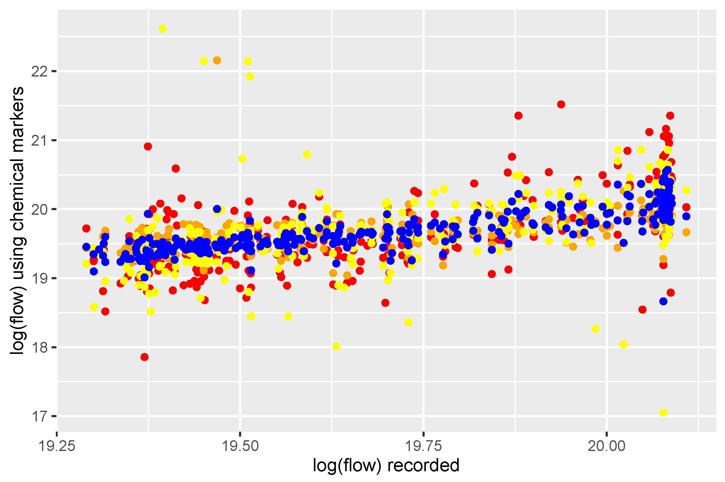
As expected, there are linear relationships between chemical markers and inverted flow, though with significant quantities of noise (Figure 2). These results show that there is not a `best’ marker to use as a proxy for the inverse flow, and a combination of markers is required for a robust proxy. Wilde et al. gives some details of the advantages and disadvantages of each marker.

2.1. Populations

The population contributing to each wastewater sample is estimated using the population within the respective sewershed (wastewater catchment that drains into a wastewater treatment plant). Lower Layer Super Output Area (LSOA) population estimates for 2020 were used, obtained from the Office for National Statistics (ONS). For each sewershed we identified the built-up areas it encompassed, and then distributed the population of each LSOA across the built-up areas it contains. While this approach provides a good estimate for the static population of a sewershed, it does not account for natural fluctuations in the population coming from sources such as commuting or tourism. We use the same values reported in Wilde et al.

3. Credibility of flow measurements for determining dilution

In Wales, surface run-off and domestic wastewater are transported in the same networks, referred to as combined sewers. Therefore, during periods of high rainfall the capacity of the sewer network can be exceeded. To prevent excess wastewater from backing up into properties, networks contain wastewater storage tanks, to smooth surges in flow, and CSOs, which allow excess flow to spill into water bodies such as rivers.

When CSOs are active the wastewater entering the treatment plant will be more dilute than indicated by the flow at the inlet. The effect of storage tanks is more subtle. Storing and then releasing wastewater does not invalidate the relation between dilution and inlet flow, but it does effect the time that the SARS-CoV-2 particles have been in transit before being measured. RNA degrades over time, therefore the delay in SARS-CoV-2 particles reaching the WWTP caused by storage tanks will reduce the yield of detectable RNA produced per person. More generally, the topography of the sewer network draining to a treatment plant will also be a factor in the degradation of RNA before samples are collected, with wastewater in larger catchments like Cardiff having to travel, on average, further distances. We will assume that this effect is independent of flow, but will make no assumptions about how it varies from one network to another.

In Wilde et al. [17] flow measurements were considered to give a reliable estimate of dilution when the flow was between the 10th and 40th percentiles (using measurements from the preceding year). The upper limit is to preclude measurements when CSOs and storage tanks are active, and the lower limit is to avoid irregularities in the transport of solids through the sewer network when the flow is very low. The upper limit is necessarily conservative, because CSO activity can be short-term but our flow measurements are at the daily scale, so CSOs may have been active even on days with moderate flow measurements.

DCWW monitors how often CSOs spill and the duration they are active (but not their flow), and in this study we use this information to determine when flow measurements reflect wastewater dilution. CSOs were matched to their respective wastewater sewershed using their physical location, then, for each WWTP, total daily active CSO time was calculated. This was then scaled to [0, 1] giving a measure of daily CSO activity at each location (Figure 3). Flow measurements within the historic 10th and 40th percentiles—those considered reliable by Wilde et al.—mostly correspond to days with low CSO activity, but not always. Instead of using these limits, we instead consider flow measurements reliable if CSO activity is below 0.01 (that is, at least 100 times less than the maximum recorded CSO activity) while retaining the requirement that the flow has to be above the 10th percentile. In doing so, 60% of the flow data is deemed reliable, compared to 30% using the previous limits.

Data on when storage tanks are active is not available, however it is assumed that they are active when CSOs are active, so the flow measurements we consider reliable here should not be much affected by storage tanks.

4. Model

Each site is modelled separately. It is helpful to distinguish between our physical model for the system and our statistical model for what is observed. For the underlying physical model our variables are:

$z^{f} (t)$: count of SARS-CoV-2 gene copies per litre at time t;
$z^{p} (t)$: count of SARS-CoV-2 gene copies per person at time t;
$m^{j, f} (t)$: level of chemical marker j per litre at time t;
$m^{j, p}$: level of chemical marker j per person (constant in time);
$f (t)$: effective flow at time t;
p: number of people contributing to effective flow (constant in time).

Our physical model is then

\begin{matrix} z^{f} (t) & = & \frac{z^{p} (t) p}{f (t)} \\ m^{j, f} (t) & = & \frac{m^{j, p} p}{f (t)} for each j . \end{matrix}

We suppose that for any given site we have the following observations, at times

t_{i}

for

i = 1, \dots n

$Y_{i}$: observed $log z^{f} (t_{i})$ ;
$L_{i}^{j}$: observed $log m^{j, f} (t_{i})$ ;
$E_{i}$: observed $log f (t_{i})$ when $r_{i} = 1$ .

Here

r_{i}

is just an indicator for the availability of flow measurements. Our statistical model supposes independent normal measurement errors on the log scale. That is, for some

σ_{Y}^{2}

σ_{L^{j}}^{2}

and

σ_{E}^{2}

, we have

\begin{matrix} Y_{i} & \sim & N (log z^{f} (t_{i}), σ_{Y}^{2}) = N (log z^{p} (t_{i}) + log p - log f (t_{i}), σ_{Y}^{2}) \\ L_{i}^{j} & \sim & N (log m^{j, f} (t_{i}), σ_{L^{j}}^{2}) = N (log m^{j, p} + log p - log f (t_{i}), σ_{L^{j}}^{2}) \\ E_{i} & \sim & N (log f (t_{i}), σ_{E}^{2}) \end{matrix}

(1)

Thus when

r_{i} = 1

Y_{i}

will give a direct unbiased estimate of

log z^{p} (t_{i})

, but when

r_{i} = 0

we need to use the

L_{i}^{j}

to estimate

log f (t_{i})

and from that obtain an estimate of

log z^{p} (t_{i})

. p is considered known so does not contribute any uncertainty.

The underlying SARS-CoV-2 prevalence will vary continuously over time, which needs to be incorporated into the model. To impose continuity on

z^{p} (t)

we model it as a Brownian motion on the log scale (at least at the time scale of the observations), that is for some

σ_{z^{p}}^{2}

we have

log z^{p} (t_{i + 1}) - log z^{p} (t_{i}) \sim N (0, σ_{z^{p}}^{2} (t_{i + 1} - t_{i})) .

Our goal is to estimate the parameters

z^{p} (t_{i})

and

f (t_{i})

for

i = 1, \dots, n

. Our other parameters are

m^{j, p}

σ_{Y}

σ_{L^{j}}

σ_{E}

and

σ_{z^{p}}

. Of these

σ_{z^{p}}

will be fixed a-priori as it is effectively a user-specified smoothing parameter, but the others will have to be estimated. Using a Bayesian approach Equations 1 specify the likelihood of the observations (

Y_{i}

L_{i}^{j}

E_{i}

) conditioned on the unobserved parameters (

log z^{p} (t_{i})

log f (t_{i})

m^{j, p}

σ_{Y}

σ_{L^{j}}

σ_{E}

). We specify priors for these parameters then calculate their posterior distributions conditioned on the observations.

For the location parameters

log z^{p} (t_{i})

log f (t_{i})

and

m^{j, p}

we use improper flat priors. For the scale parameters

σ_{Y}

σ_{L^{j}}

and

σ_{E}

we use either Half-Cauchy priors, or Inverse-Gamma priors when some regularisation is required.

4.1. Missing and censored observations

Missing observations of

L_{i}^{j}

and

E_{i}

are inherent in the data, and the

Y_{i}

and

L_{i}^{j}

can also be below their LOD, in which case they are censored. The Bayesian methodology implicitly allows for missing and censored observations. Missing values simply do not contribute to our posterior estimates, while for censored observations the likelihood of the observation is replaced with the likelihood integrated over the censored region. Thus for any time point i, provided we have at least one

L_{i}^{j}

E_{i}

, we will in theory have some information about the posteriors of

f (t_{i})

and

log z^{p} (t_{i})

. In practice, however, if we do not have at least one

L_{i}^{j}

it is hard to distinguish between the variation in

Y_{i}

and

E_{i}

, and when we sample from the posterior we can get very small (and disruptive) values of

σ_{Y}

. For this reason, when there are missing and/or censored values of

L_{i}^{j}

(in addition to the missing flow observations), it necessary to use a regularising Inverse-Gamma(1,1) prior for

σ_{Y}

4.2. Smoothing

By incorporating continuity into our model, we smooth our estimate of the SARS-CoV-2 prevalence, which also serves to regulate our estimate for the flow. In Figure 4 we illustrate the effect of

σ_{z^{p}}

on the amount of smoothing. The data has very little information about

σ_{z^{p}}

and we have treated it as a fixed user-determined smoothing parameter. In Wilde et al. [17] a ten-point moving average smooth was used, with the lag chosen based on a 5-day sampling week. For our results we have used

σ_{z^{p}} = 0.5

, which results in the posterior medians of the

log z^{p} (t_{i})

having the same range as the estimates obtained using the method of Wilde et al. A quantitative approach to the choice of

σ_{z^{p}}

would require independent estimates of

log z^{p} (t_{i})

, for example estimates from the U.K. Coronavirus (COVID-19) Infection Survey. Unfortunately, these data were not available to us at the required granularity of individual sewersheds.

5. Results and discussion

The model was implemented using the Stan modelling language and RStan [13,14]. Posterior samples were generated using Hamiltonian Monte Carlo with the No-U-Turn-Sampler (NUTS). For each location we used 4 chains with 20,000 warm-up iterations and 20,000 sampling iterations. The MCMC-nuts diagnostics from the bayesplot package [4] were used to check that the samples were reliable.

After exploring multiple smoothing options (Figure 4), the smoothing parameter

σ_{z^{p}}

was fixed at

0.5

, which is the value for which the range of our estimates matches the range of estimates reported using the current methodology.

The posterior medians for the count of SARS-CoV-2 gene copies per person produced by the methods presented in this study are in close agreement to those obtained using the methodology of Wilde et al. [17], with the exception that the latter suffers from a small lag (Figure 5). This is because the existing method uses a 10-point moving average smooth, which necessarily slows down how quickly it responds to changes in

z^{p} (t)

To compare the relative worth of the different chemical markers, we used the posterior medians of the

log m^{j, p}

to give separate naïve estimates of the log flow using individual markers for the normalisation. That is, using the j-th marker we have

\hat{log f (t_{i})} = \hat{log m^{j, p}} + log p - L_{i}^{j} .

The results showed that orthophosphate-based estimates were the most variable and conductivity based estimates the least variable (Figure 6), which is consistent with the correlations reported in Figure 2. Information like this is important for deciding which chemical marker to adopt when initiating or streamlining a wastewater monitoring programme. Of the three chemical markers we used, conductivity was the most useful as it provided the least variable estimates, and it can be measured in real time in the field with relative ease. Choosing a chemical marker for flow estimation will be context dependant, for example, conductivity can be sensitive to saltwater ingress into the WWTP, but the results shown here show that conductivity is a promising first candidate.

The normalised estimates of SARS-CoV-2 prevalence constructed here are consistent with the methodology currently in use by the WeWASH project for reporting to the Welsh Government, as outlined by Wilde et al. However, the new methodology has the added advantage of credible intervals. These are particularly valuable for WBE of biological markers such as SARS-CoV-2 because they provide health professionals and policy makers with an indication of confidence in the signal trends that are being presented, which is lacking from the current approach. In addition, the methodology presented in this study does not have the disadvantage of a response lag that comes from a moving average smooth. Removal of this lag is valuable because data driven decision making for infectious diseases such as SARS-CoV-2 relies on timely interventions, an advantage often attributed to WBE (Levy et al. [8]). Some elements of WBE will always introduce a lag time between an individual becoming infected and their detection, such as wastewater transit time to the WWTP as well as collection and analysis of samples. However, if lag times can be avoided elsewhere, this will improve how representative trends are of the current spread of infectious disease.

Our proposed methodology also deals with missing and censored values where the current methodology failed. Measuring biological markers such as SARS-CoV-2 gene copies in wastewater can be difficult. RNA is ephemeral and wastewater is a complex matrix, containing RT-qPCR inhibitors such as polysaccharides, bile salts, lipid, urate, fulvic and humic acids, metal ions, algae and polyphenols (Scott et al. [12]). While laboratory processes aim to remove these inhibitors, they can still have an effect, including sample dropouts and values falling below the LOD (that is, censored values). In addition to this, sampling the wastewater itself can present issues, such as ragging, temporary access issues and equipment failure, which can result in short periods of missing values. Therefore, being able to include information on missing and censored values in the Bayesian model is of value.

Another benefit of the new approach presented here is that it optimally weights the dilution proxies from each of the chemical markers, unlike the current methodology which either gives them equal weight or omits them. Such functionality is important for accounting for dilution because it is possible that markers may become less representative over time, both on a seasonal basis and more long term. For example, the application of de-icing salt on roads and runoff into wastewater could inflate conductivity in the winter season, to a point where it is no longer representative of dilution, but this problem would not be encountered in the summer (Koryak et al. [6]). Long term changes of land use in the catchment could also impact how representative certain chemical markers are of dilution. For example, the establishment of a food processing industry within a catchment could see ammonia levels be intermittently inflated (Brennan et al. [2]), and less representative of dilution.

While this study has focused on the dilution of SARS-CoV-2, the methodology outlined in this study is not limited to one biological marker. Wastewater surveillance programmes sample many other biological markers of infectious disease, which will also all benefit from the advantages of this new approach. The WEWASH programme alone also monitors norovirus, influenza and enterovirus. Beyond biological markers, comprehensively accounting for dilution is also important for chemical compounds of interest, such as emerging pollutants, legacy pollutants and illicit drugs.

In conclusion, our new methodology, used to account for wastewater dilution using chemical markers, is robust when compared to previous methods aimed at doing the same thing, but contains a suite of additional benefits. These benefits include credible intervals for estimates, model-based smoothing without lags, systematic handling of missing/censored values, and optimal weighting of chemical markers. Improvements such as these are concordant with the aims of WBE more broadly, producing more representative and robust insights for public health practitioners and policy makers.

Author Contributions

Methodology, O.D.J. and H.W.; formal analysis and software, O.D.J.; data curation, A.J.B. and W.B.P.; writing—original draft preparation, O.D.J. and W.B.P.; writing—review and editing, O.D.J., A.J.B., W.B.P., H.W. and I.D.; funding, O.D.J., I.D., D.L.J. and A.W. All authors have read and agreed to the published version of the manuscript.

Funding

This work was funded by the Welsh Government under the Welsh Wastewater Programme (C035/2021/2022/2033).

Data Availability Statement

Owing to the sensitive nature of the materials under study, the data used in this manuscript is subject to a confidentiality agreement and cannot be made available.

Acknowledgments

The authors wish to thank their collaborators from PHW, DCWW and Hafren Dyfrdwy for their cooperation and essential support to the WEWASH project.

Conflicts of Interest

The authors declare no conflicts of interest. The funders had no role in the design of the study, in the collection, analyses, or interpretation of data, in the writing of the manuscript, or in the decision to publish the results.

Abbreviations

COVID-19	Coronavirus disease 2019
CSO	Combined sewer overflow
DCWW	Dwr Cymru Welsh Water
LSOA	Lower Layer Super Output Area
MCERTS	Monitoring Certification Scheme
ONS	Office for National Statistics
PHW	Public Health Wales
RNA	Ribonucleic acid
RT-qPCR	Quantitative reverse transcription polymerase chain reaction
SARS-CoV-2	Severe acute respiratory syndrome coronavirus 2019
WBE	Wastewater-based epidemiology
WEWASH	Wales Environmental Wastewater Analysis and Surveillance for Health
WWTP	Wastewater treatment plant

References

Been, F., Rossi, L., Ort, C., Rudaz, S., Delémont, O., Esseiva, P. Population normalization with ammonium in wastewater-based epidemiology: Application to illicit drug monitoring. Environ. Sci. Technol. 2014, 48:8162–8169. [CrossRef]
Brennan, B., Lawler, J., Regan, F. Recovery of viable ammonia–nitrogen products from agricultural slaughterhouse wastewater by membrane contactors: a review. Environ. Sci. Water Res. Technol. 2021, 7:259–273. [CrossRef]
Farkas, K., Hillary, L.S., Thorpe, J., Walker, D.I., Lowther, J.A., McDonald, J.E., Malham, S.K., Jones, D.L. Concentration and Quantification of SARS-CoV-2 RNA in Wastewater Using Polyethylene Glycol-Based Concentration and qRT-PCR. Methods Protoc. 2021, 4:17. [CrossRef]
Gabry, J., Simpson, D., Vehtari, A., Betancourt, M., Gelman, A. Visualization in Bayesian workflow. J. R. Stat. Soc. A 2019, 182:389–402. [CrossRef]
Jones, D.L., Baluja, M.Q., Graham, D.W., Corbishley, A., McDonald, J.E., Malham, S.K., Hillary, L.S., Connor, T.R., Gaze, W.H., Moura, I.B., Wilcox, M.H., Farkas, K. Shedding of SARS-CoV-2 in feces and urine and its potential role in person-to-person transmission and the environment-based spread of COVID-19. Sci. Total Environ. 2020, 749:141364. [CrossRef]
Koryak, M., Stafford, L.J., Reilly, R.J., Magnuson, P.M. Highway Deicing Salt Runoff Events and Major Ion Concentrations along a Small Urban Stream. J. Freshw. Ecol. 2001, 16:125–134. [CrossRef]
Langeveld, J., Schilperoort, R., Heijnen, L., Elsinga, G., Schapendonk, C.E.M., Fanoy, E., de Schepper, E.I.T., Koopmans, M.P.G., de Graaf, M., Medema, G. Normalisation of SARS-CoV-2 concentrations in wastewater: The use of flow, electrical conductivity and crAssphage. Sci. Total Environ. 2023, 865:161196. [CrossRef]
Levy, J.I., Andersen, K.G., Knight, R., Karthikeyan, S. Wastewater surveillance for public health. Science 2023, 379:26–27. [CrossRef]
Naughton, C.C., Roman, F.A., Alvarado, A.G.F., Tariqi, A.Q., Deeming, M.A., Kadonsky, K.F., Bibby, K., Bivins, A., Medema, G., Ahmed, W., Katsivelis, P., Allan, V., Sinclair, R., Rose, J.B. Show us the data: global COVID-19 wastewater monitoring efforts, equity, and gaps. FEMS Microbes 2023, 4:1–8. [CrossRef]
Perry, W.B., Ahmadian, R., Munday, M., Jones, O., Ormerod, S.J., Durance, I. Addressing the challenges of combined sewer overflows. Environ. Pollut. 2024, 343:123225. [CrossRef]
Perry, W.B., Chrispim, M.C., Barbosa, M.R.F., de Souza Lauretto, M., Razzolini, M.T.P., Nardocci, A.C., Jones, O., Jones, D.L., Weightman, A., Sato, M.I.Z., Montagner, C., Durance, I. Cross-continental comparative experiences of wastewater surveillance and a vision for the 21st century. Sci. Total Environ. 2024, 170842. [CrossRef]
Scott, G., Evens, N., Porter, J., Walker, D.I. The Inhibition and Variability of Two Different RT-qPCR Assays Used for Quantifying SARS-CoV-2 RNA in Wastewater. Food Environ. Virol. 2023, 15:71–81. [CrossRef]
Stan Development Team. RStan: the R interface to Stan. R package version 2.32.5 2024. https://mc-stan.org.
Stan Development Team. Stan Modeling Language Users Guide and Reference Manual. Version 2.34 2022. https://mc-stan.org.
Sweetapple, C., Melville-Shreeve, P., Chen, A.S., Grimsley, J.M.S., Bunce, J.T., Gaze, W., Fielding, S., Wade, M.J. Building knowledge of university campus population dynamics to enhance near-to-source sewage surveillance for SARS-CoV-2 detection. Sci. Total Environ. 2022 806:150406. [CrossRef]
Wade, M.J., Jacomo, A.L., Armenise, E., Brown, M.R., Bunce, J.T., Cameron, G.J., Fang, Z., Farkas, K., Gilpin, D.F., Graham, D.W. Understanding and managing uncertainty and variability for wastewater monitoring beyond the pandemic: Lessons learned from the United Kingdom national COVID-19 surveillance programmes. J. Hazard. Mater. 2022, 424:127456. [CrossRef]
Wilde, H., Perry, W.B., Jones, O., Kille, P., Weightman, A., Jones, D.L., Cross, G., Durance, I. Accounting for Dilution of SARS-CoV-2 in Wastewater Samples Using Physico-Chemical Markers. Water 2022, 14:2885. [CrossRef]

Figure 1. SARS-CoV-2 gene copies per litre and flow (litres) measured at Cardiff Bay from 2022-01-01 to 2023-03-31. The bottom panel gives the naïve SARS-CoV-2 count per person obtained by normalising using the raw flow measurements.

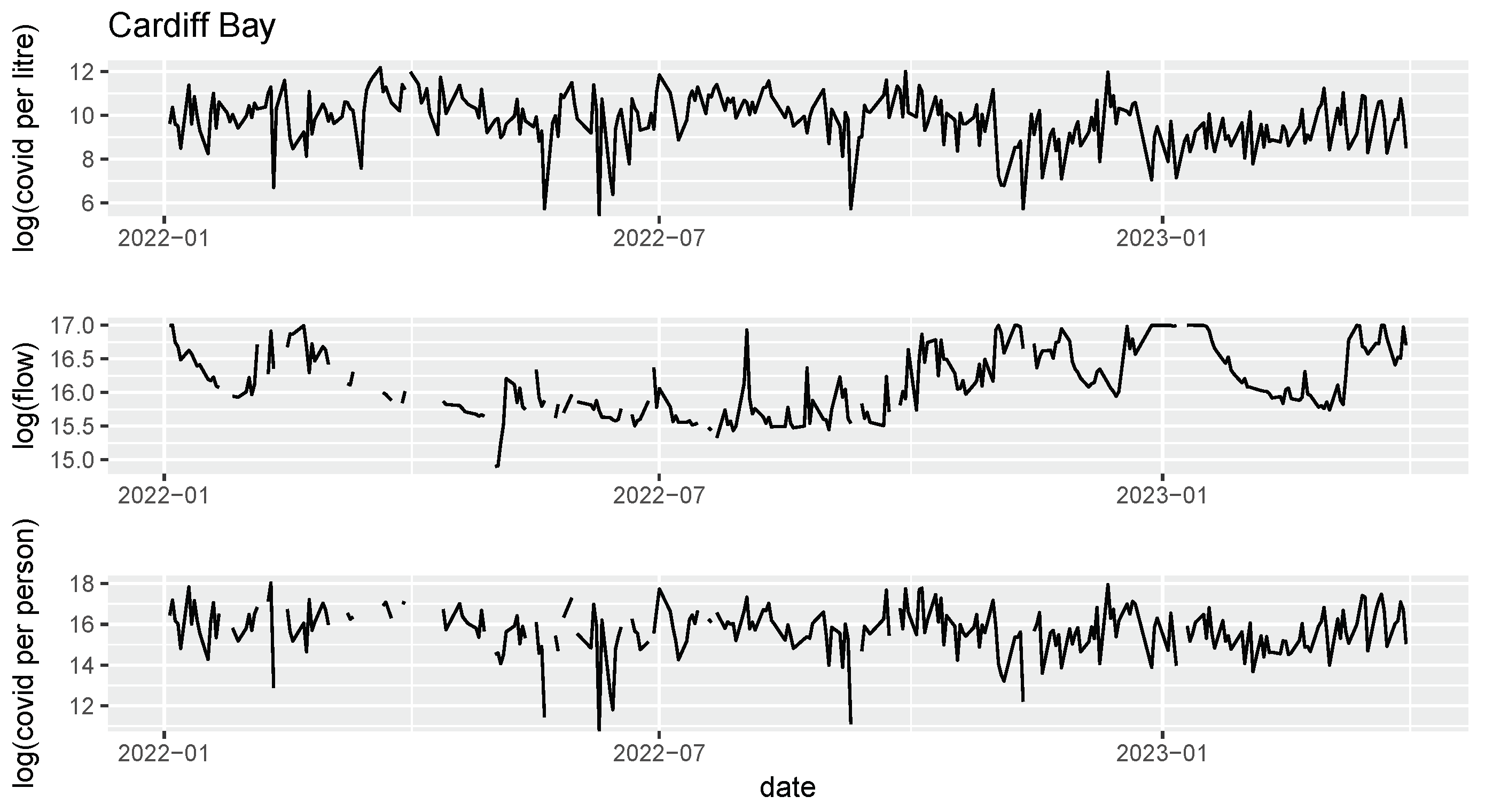
Figure 2. Pairs plot comparing the inverse flow and the chemical markers ammonia, orthophosphate, and conductivity. Samples taken from the Cardiff Bay wastewater treatment plant, 2022-01-01 to 2023-03-31.

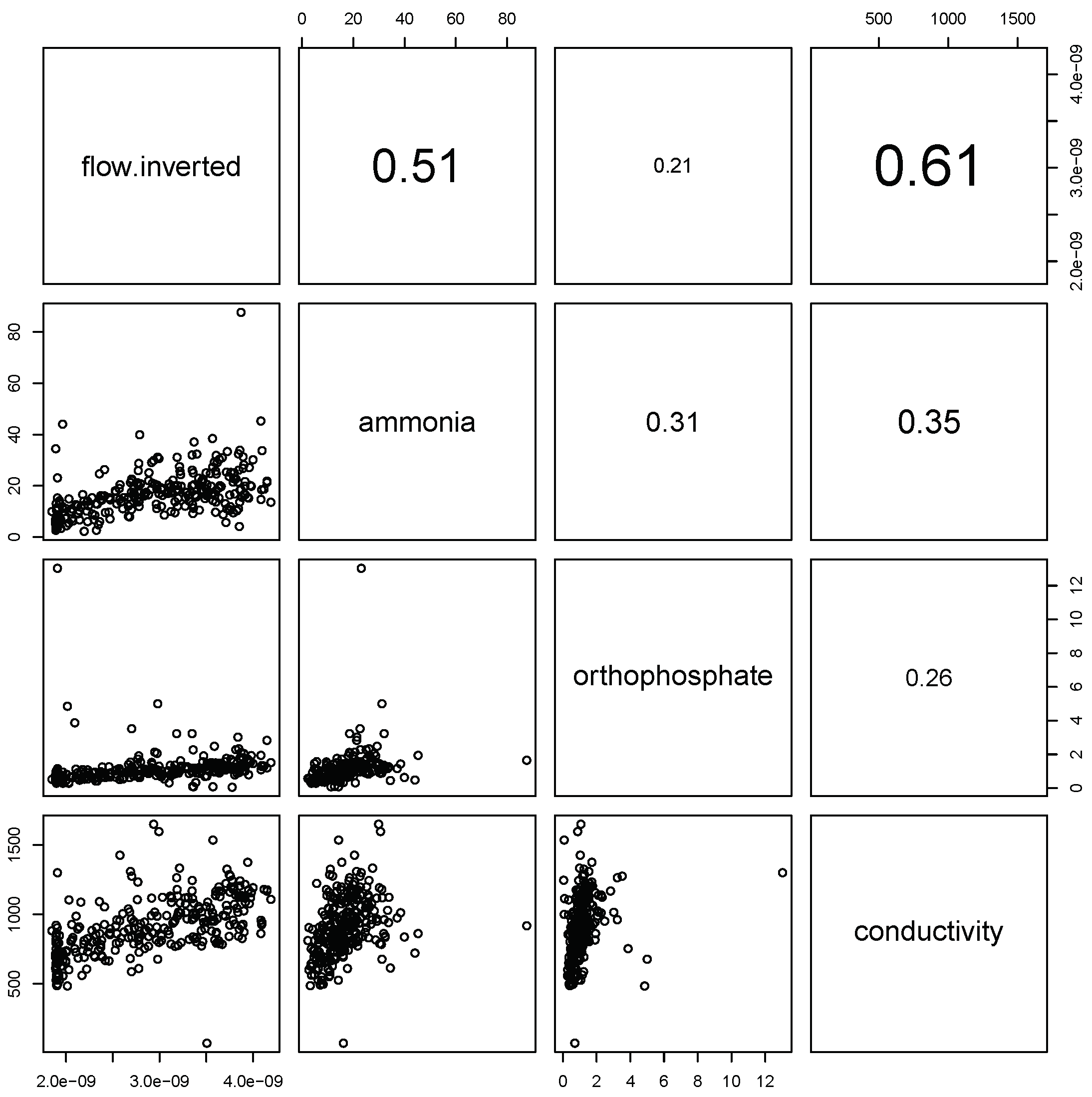
Figure 3. CSO activity against measured flow at each of the locations we consider. Flow values within historic 10th and 40th percentiles are in red.

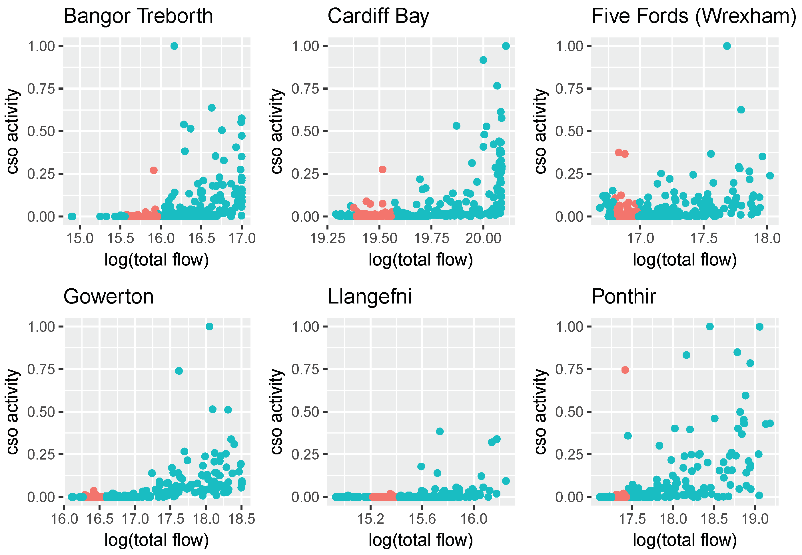
Figure 4. Posterior medians of

log z^{p} (t_{i})

(that is, a smoothed count of SARS-CoV-2 gene copies per person) for

σ_{z^{p}} = 0.1

(orange),

0.5

(red), and 1 (purple). These results are from the Five Fords (Wrexham) sampling location, from 2023-01-01 to 2023-03-31.

Figure 4. Posterior medians of

log z^{p} (t_{i})

(that is, a smoothed count of SARS-CoV-2 gene copies per person) for

σ_{z^{p}} = 0.1

(orange),

0.5

(red), and 1 (purple). These results are from the Five Fords (Wrexham) sampling location, from 2023-01-01 to 2023-03-31.

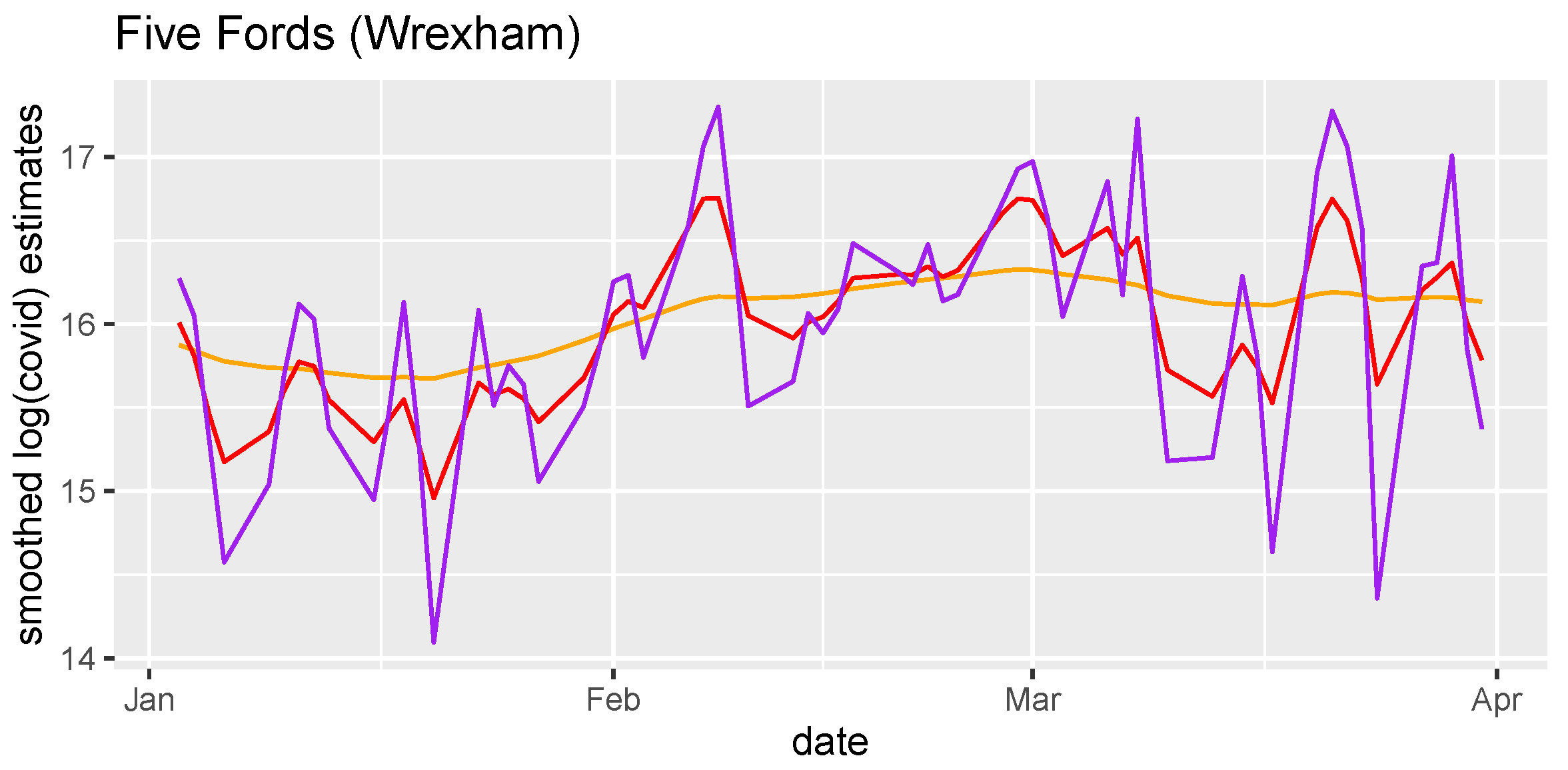
Figure 5. Posterior medians and 95% credible intervals (red) for the

log z^{p} (t_{i})

(that is, the smoothed count of SARS-CoV-2 gene copies per person) at each of the six sampling locations. Estimates obtained using the method of Wilde et al. [17] are given in grey.

Figure 5. Posterior medians and 95% credible intervals (red) for the

log z^{p} (t_{i})

(that is, the smoothed count of SARS-CoV-2 gene copies per person) at each of the six sampling locations. Estimates obtained using the method of Wilde et al. [17] are given in grey.

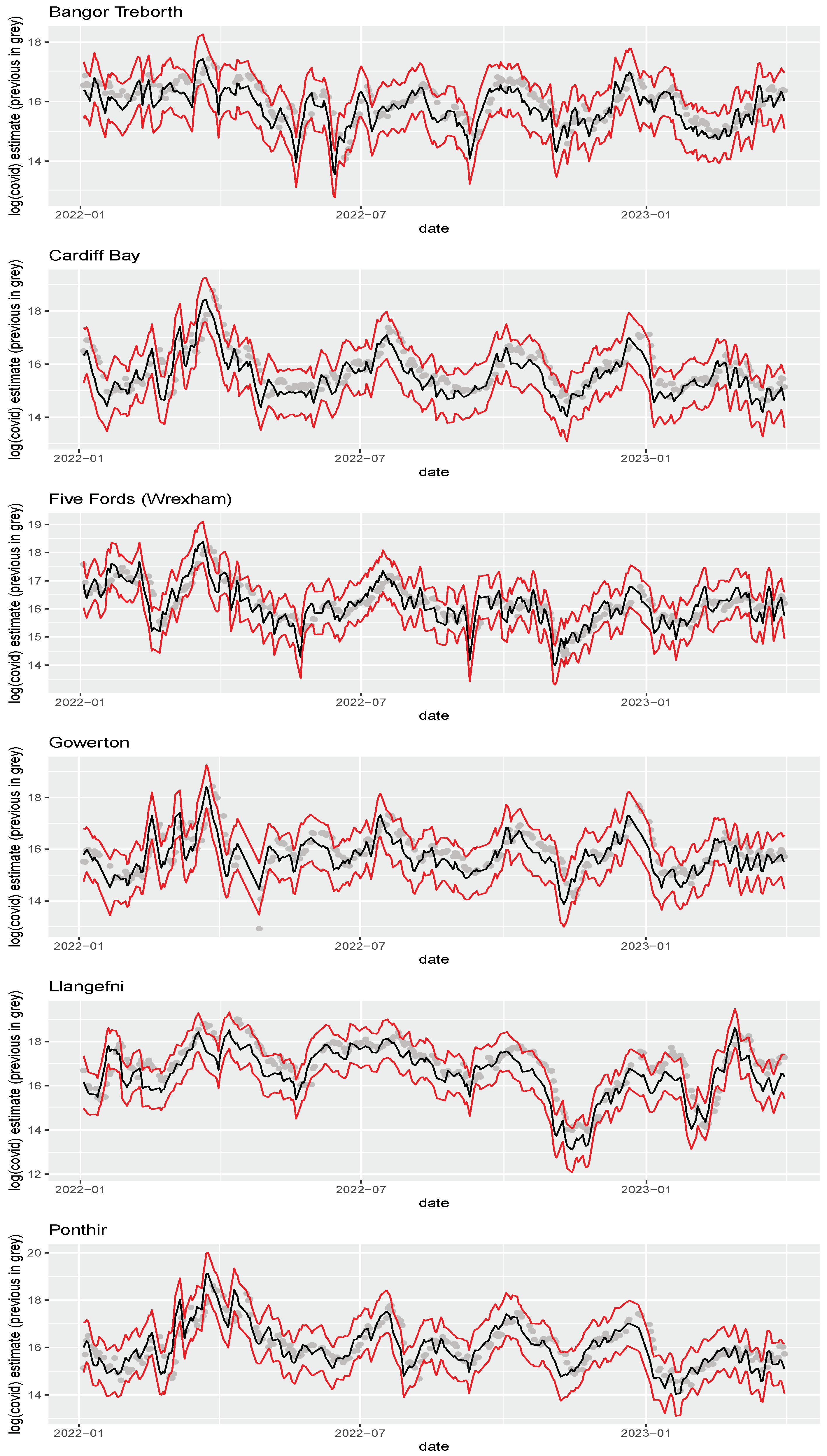
Figure 6. Naïve flow estimates using individual chemical markers: ammonia in red, conductivity in orange, and orthophosphate in yellow. Posterior medians of the log flow are given in blue for comparison. Data from the Cardiff Bay WWTP.

Disclaimer/Publisher’s Note: The statements, opinions and data contained in all publications are solely those of the individual author(s) and contributor(s) and not of MDPI and/or the editor(s). MDPI and/or the editor(s) disclaim responsibility for any injury to people or property resulting from any ideas, methods, instructions or products referred to in the content.

© 2024 by the authors. Licensee MDPI, Basel, Switzerland. This article is an open access article distributed under the terms and conditions of the Creative Commons Attribution (CC BY) license (http://creativecommons.org/licenses/by/4.0/).

Copyright: This open access article is published under a Creative Commons CC BY 4.0 license, which permit the free download, distribution, and reuse, provided that the author and preprint are cited in any reuse.

Downloads

211

Views

Comments

Subscription

Notify me about updates to this article or when a peer-reviewed version is published.

MDPI Initiatives

Important Links

Choose an area of interest and we will send you notifications of new preprints at your preferred frequency.

Disclaimer