
Submitted:
12 February 2024
Posted:
12 February 2024
You are already at the latest version
Abstract
Structures inevitably suffer damages after an earthquake, with their severity ranging from minimal damages to non-structural elements to partial or even total collapse, possibly with loss of human lives. Thus, it is essential for engineers to understand the crucial factors that drive a structure towards suffering higher degrees of damage, so that preventative measures can be taken. In the present study, we focus on three well-known damage thresholds, namely Collapse Limit State, Ultimate Limit State and Serviceability Limit State and analyze which of the features obtained via Rapid Visual Screening, determine whether or not a given structure will cross that threshold. To this end, we use Machine Learning to perform binary classification for each damage threshold, as well as Explainability via SHAP values (acronym for SHapley Additive exPlanations) to quantify the effect of each parameter. The quantitative results obtained demonstrate the potential applicability of ML methods to re-calibrate the computation of structural vulnerability indices using data from recent earthquakes.
Keywords:
Rapid Visual Screening
; Explainable AI
; Feature Importance
; SHAP
1. Introduction
During the last decades, due to the large number of existing building stock, engineering focus has shifted from analyzing and designing new structures to maintaining the preexisting buildings to modern standards of safety and serviceability [1]. As is well known, the results of an earthquake can be catastrophic to the society in terms of loss of human lives and requirements for large monetary reparations, with some examples including the Turkey (Izmit) 1999, Athens 1999, Pakistan 2005 and the 2023 Turkey earthquakes.
Governments and authorities can take preemptive measures to mitigate these effects, however, due to obvious limitations in resources and manpower, it is not possible to do so for all existing buildings, especially in large urban areas. Thus, most countries have introduced multi-stage procedures to assess and evaluate the total potential consequences and losses from an earthquake, and thus identify the most critical structures where allocation of further resources should be prioritized.
As a first step of these methods a Rapid Visual Screening Procedure (RVSP) [2] is usually performed, wherein experts quickly inspect buildings and identify key structural characteristics that affect the overall seismic behaviour. For example, these could include whether or not the structure has short columns or soft storeys, the presence of neighboring buildings that could results in pounding effects, irregularities in the horizontal or vertical plan of the building and others [3,4]. Subsequently, these obtained characteristics are weighted to compute a seismic vulnerability index which is used to rank the structures according to their expected degree of damage [5]. Finally, the most vulnerable structures that have been identified from the aforementioned steps, are subjected to more accurate, analytical methods, such as finite element analysis. These methods are prohibitively costly and time consuming to be applied to every structure in the population, but yield an accurate assessment of the seismic vulnerability of the structures under consideration and, thus, of any potentially required preemptive measures to be applied to them.
In USA, the Federal Emergency Management Agency (FEMA) first introduced such an RVSP [2] in 1988, which has since been modified to include more structural features that affect the overall seismic performance [6]. Countries with high seismic activity, such as Japan, Italy, Canada, India or Greece, have derived similar pre-earthquake assessment, adapted to the characteristics of their respective building stocks. The success of RVSP in screening the candidate structures for further analysis heavily depends on an accurate calibration of the weights of the structural characteristics. Thus, data from major recorded earthquakes in conjunction with engineering expertise have been used in the past by researchers for this task [7,8].
On the other hand, recent years have seen an increase of the use of Machine Learning (ML) methods for the task of predicting the degree of a damage of reinforced concrete structures. Classification techniques have been previously employed to classify structures in predicted damage categories. Harichian et al. [9] employed Support Vector Machines, which they calibrated on dataset of earthquakes in four different countries. Sajan et al. [10] employed a variety of models, including Decision Trees, Random Forests, XGBoost and Logistic Regression. Similarly, regression methods have also been employed for this task. Among others, Luo and Paal [11] and Kazemi et al. [12] used ML methods to predict the interstorey drift, which can be used as a damage index.
Even though Machine Learning methods are powerful, they often lack the desired interpretability. The path a Decision Tree followed to reach its predictions can be readily visualized, but the same does not hold for more complex ML models. Thus, explainability techniques and models have been employed in ML [13] in order to analyze how these models weigh their input parameters when making a decision, thus increasing the reliability of their predictions. Among others, Mangalathu et al. [14] have recently employed Shapley additive explanations (SHAP) [15] to quantify the effect of each input parameter on damage predictions of bridges in California. Sajan et al. [10] performed multiclass classification to predict the damage category of structures. They also employed binary classification to predict whether the damage was recoverable or reconstruction was needed. Subsequently, they employed SHAP values to identify 19 of the top 20 most important features for both tasks. However, the features they employed significantly deviate from the ones in the RVS procedure and lack many of the features employed in the present study.
The features employed in the present study have been used before [16,17]. However, there is no consensus on the magnitude of the effect each feature has on the vulnerability ranking and different researchers or different seismic codes employ different values. In this paper, we implement explainable Machine Learning techniques and SHAP values to analyze features’ contribution to the relative classification of structures in the respective damage categories. To the best of our knowledge, the novelty contribution of the introduced approach is that it does not attempt to directly predict the damage category. It considers the well-known thresholds of Serviceability Limit State (SLS), Ultimate Limit State (ULS) as well as Collapse Limit State (CLS), to distinguish structures that not only surpassed the ULS threshold, but suffered partial or total collapse as well, which could potentially lead to loss of human life. Moreover, Machine Learning was used in order to develop binary classification models, capable to distinguish between adjacent damage categories.
The benefit of this modeling research effort in comparison with the previously established literature is twofold. On the one hand, the obtained binary classifiers have significantly improved accuracy, compared to previously examined models. A higher accuracy enhances the reliability of the extracted feature importance coefficients, which is the main focus of the present study. On the other hand, this binary classification approach allows us to examine each of the damage thresholds separately, and thus it answers the following questions: what were the deciding factors that led a structure that would have otherwise suffered minimal to no damages to cross the serviceability limit threshold?”. “If a structure did cross the serviceability threshold, what prevented it from crossing the ultimate limit state threshold as well?”. Finally, “if it did cross the ULS threshold, what factors prevented it from ultimately collapsing?”
2. Materials and Methods
2.1. Dataset description
The dataset used in the present study is a sample consisting of 457 structures obtained after the 1999 Athens Earthquake via Rapid Visual Screening (RVS) [16]. The selected structures had suffered damages across the spectrum, ranging from very low or minimal damages, to structures that partially or completely collapsed during the earthquake. The dataset was drawn from different geographical regions and, thus, the local conditions varied across the sample. The authors in [16] took steps to mitigate their effect on the study: when sampling from a specific local area, they sampled structures across the damage spectrum. The degree of damage was labeled using 4 categories, specifically:
- “Black”: Structures that suffered total or partial collapse during the earthquake, potentially leading to loss of human life.
- “Red”: Structures with significant damages to their structural members.
- “Yellow”: Structures with moderate damages to the structural members and potentially including extended damages to non-structural elements.
- “Green”: Structures that suffered very little or no damages at all.
The distribution of structures across the above damage categories is shown in Figure 2.
For each structure, a set of attributes were documented, specifically:
- Free ground level (Pilotis), soft storeys and/or short columns: In general, this attribute pertains to structures wherein a storey has significantly less structural rigidity than the rest. For example, this can manifest on the ground floor (pilotis) when it has greater height than the typical structure storey, or when the wall fillings do not cover the whole height of a storey, effectively reducing the active height of the adjacent columns.
- Wall fillings regularity: This indicated whether the non-bearing walls were of sufficient thickness and with few openings. The presence of such wall fillings is beneficial to its overall seismic response.
- Absence of design Seismic codes: This pertained to pre-1960 structures, which were not designed following a dedicated seismic code.
- Poor condition: Very high or non-uniform ground sinking, concrete with aggregate segregation or erosion, or corrosion in the reinforcement bars are examples of maintenance related factors that can reduce the seismic capacity of the building.
- Previous damages: This pertained to structures which had suffered previous earthquake damages that had not been adequately repaired.
- Significant height: This described structures with 5 or more storeys.
- Irregularity in-height: This described structures with a discontinuity in the vertical path of the loads.
- Irregularity in-plan: This pertained to structures with floor plan that significantly deviated from being a rectangle, e.g. floor plans with highly acute angles in their outer walls, or E, Z, or H-shaped.
- Torsion: This affected structures with high horizontal eccentricity, which are subjected to torsion during the earthquake.
- Pounding: If adjacent buildings do not have a sufficient gap between them and especially if they have different heights, then the floor slabs of one building can ram into the columns of the other.
- Heavy non-structural elements: If such elements are displaced during the earthquake they can potentially create eccentricities, leading to additional torsion.
- Foundation Soil: The Greek Code for Seismic Resistant Structures - EAK 200 [3] classifies soils into categories A, B, C, D and X. Class A refers to rock or semi-rock formations extending in wide area and large depth. Class B refers to strongly weathered rocks or soils, mechanically equivalent to granular materials. Classes C and D refer to granular materials and soft clay respectively, while class X refers to loose fine-grained silt [3]. In [16] and in the present study, soils in EAK category A are classified as S1, category B is classified as S2. Soils in EAK category C, D and X were not encountered.
- The design Seismic Code: This feature described the Seismic Codes the structures adhered to at the time of their design. Specifically, structures that were built before 1984 were classified as RC1, buildings constructed between 1985 and 1994 were labeled RC2 and, finally, building constructed after 1995 were labeled RC3, as the Greek state introduced updated Seismic Codes at these milestones.
Note that most of the above features were binary, i.e., a Yes/No statement was given about whether or not the structure displayed the relevant feature. We transformed these to Boolean values, i.e., . The design Seismic Code was transformed to an integer value, i.e., . Finally, in 452 out of the 457 total documents, the authors in [16] noted the exact number of storeys instead of whether or not this was . Given that this was deemed more informative, we opted to disregard these structures ( of the sample) and use this feature instead.
2.2. Data preprocessing
The core of the designed and employed modeling effort lies in the development of a Machine Learning (ML) model for binary classification that, given a pair of structures with corresponding feature vectors , is capable of predicting whether should rank higher than or vice versa [18].
However, it can be readily observed from Figure 2 that the “Red” label heavily dominates the sampled dataset. This so-called “class imbalance problem” has significant adverse effects on any Machine Learning algorithm [19,20,21,22]. It leads the model to be skewed towards the majority class, creating bias and rendering the algorithm unable to adapt to the features of the minority classes [19,20]. This imbalance can be treated with undersampling the majority class, and there are numerous methods in the literature in order to do so [23,24,25]. These methods include randomly selecting a subset of the samples in the majority class [26,27], or model based methods, such as NearMiss, Tomek Links, or Edited Nearest Neighbours [23,24,25]. NearMiss-2 was found to perform better by the authors and it is what will be using in the sequel. Using the above, we undersampled the majority class by a factor of , in order to achieve a relative class balance, which, as was mentioned, is crucial to the performance of the machine learning algorithms. The distribution of structures across the above damage categories after undersampling is shown in Figure 3.
Now, in order to represent the pair using a single feature vector as input for the Machine Learning model, we considered the pairwise transformation with . Other pairwise transformations can be employed, e.g. , with , i.e., appending to [28]. However, the transformation employed in the present study has the advantage of a more natural interpretation, which is the goal of this study. For a example, a value in the transformed dataset of 2 storeys indicates that structure had 2 more storeys than . Similarly, a transformed value of for the “pounding” attribute indicates that suffered from it, while did not.
A similar transformation was applied to the labels of the damage categories. To this end, the labels where first ranked in ascending order, i.e., Green, Yellow, Red, Black. Then, for a pair of structures with and , the transformed target variable was , where denotes the sign function. Thus, for example, a transformed variable of indicates that suffered more severe damages than . It is a fact that the focus of this research is to gauge the contribution of the involved parameters to the extend of a structure’s relative damage. Therefore, pairs with were not included in the transformed dataset.
2.3. Machine Learning Algorithm
In order to analyze the importance of each feature for the relative classification of each pair of structures, we considered 3 different pairings of structures. Specifically, we considered the subset consisting of the (Green, Yellow), (Yellow, Red) and (Red, Black) structures. We did this because each of the labels has a very distinct definition: The Black and Red structures correspond to the Collapse state and Ultimate Limit State (ULS) respectively, while Yellow corresponds to the Serviceability Limit State (SLS). Thus, by using this pairing, our models will learn to distinguish adjacent damage states and the features that lead to this increase in the suffered damages. For each of these pairs, we performed the pairwise transformations presented above. The number of structures in each pair as well as in each transformed dataset is shown in Table 1.
For each of the above pairs, we constructed a binary classifier as described in Section 2.2. The subsequent analysis on the importance of the features of these classifiers will help us answer questions like“what were the deciding factors that led a structure to be Red and not Yellow, to cross ULS and suffer heavy damages, instead of only crossing SLS and suffering moderate damages?”. There are many classifiers available in the literature to perform this task. The authors in [18] worked on the same dataset and analyzed a variety of models. The best performing one was found to be the Gradient Boosting (GB) Classifier [29], which is what we will be employing in the sequel. GB is a powerful method that learns a classifier incrementally, starting from a base model. Specifically, it learns a function
where are the individual “weak” models (Decision Trees [30]) that the algorithm learns at each iteration with their parameters , N is the user defined number of these models and are the learned weights that produce the final linear combination. The steps of the method are shown in Algorithm 1 [31]. The algorithm was implemented in Python programming language, using the Machine Learning library scikit-learn [32].
| Algorithm 1 Gradient Boosting learning process [31]. |
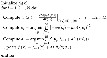 |
In the above, is the loss function that measures the error between the predictions and the true values, M is the number of samples the model is trained on and is a so-called “learning rate”, which modifies the contribution of each individual Tree [33].
2.4. Hyperparameter tuning
As is evident from (1) and Algorithm 1, Gradient Boosting learns a number of parameters during its training, e.g. the weights . However, there are a number of so-called hyperparameters, i.e., parameters set by the user before training begins, such as the number N of the individual Decision Trees, or the maximum allowed depth of each tree. The configuration of these hyperparameters can reduce overfitting [34,35] and has a direct impact on the overall accuracy of the model [36].
Thus, it becomes clear the importance of an appropriate tuning of these hyperparameters to achieve optimal results. This has led to a variety of methods to address this, with some reviews of the existing algorithms given by Yu and Zhu [37] or Yang and Shami [36]. In this paper, we opted for Bayesian optimization, as it does not search the hyperparameter space blindly, but using each iteration’s results on the next one, which can lead to faster convergence to the optimal solution [38]. The implementation was carried out using the dedicated Python library scikit-optimize [39].
2.5. SHAP
A common measure in order to gauge the strength of the effect of each feature on the outcome, which is the focus of the present study, are the so-called SHapley additive exPlanations (SHAP) [15]. They are the equivalent in the Machine Learning literature of the Shapley values in cooperative game theory, introduced by Lloyd Shapley in 1951 [40]. SHAP values provide interpretability by constructing a simpler, explainable model at the local neighborhood of each point in the dataset. Thus, given a learned Machine Learning model f, a local approximation g can be formulated as follows [15]:
where in the above n is the number of features, is a binary vector whose value in the position denotes whether or not the corresponding feature was used in the prediction and denotes the SHAP value of that feature, i.e., the strength of its contribution to the model’s output.
The values of the ’s, following the notation of Lundberg et al. [41] are computed as follows: Let be the set of features used and let be a subset of N. Then, we have [41,42]
Intuitively, this corresponds to the weighted average over all feature combinations (coalitions) of the difference in the model prediction with and without the inclusion of the feature.
As it has been mentioned, the above values pertain to a specific point. Consider, for example, the pair (Red, Black). There were 102 Red structures in the undersampled dataset and 90 Black ones. This yielded pairs, i.e., samples in the transformed space, as shown in Table 1
Thus, we have a matrix , where each value is the SHAP value of the feature calculated at the sample. Thus, in order to obtain an aggregated value for the whole dataset, we used a normalized norm of each column in the matrix. We compared the results obtained using the norm (sum of absolute values), which is the most commonly used in the literature, and the well-known Euclidean norm , which increases the contribution of larger values while simultaneously reducing the effect of smaller, noisy components. Thus, for each feature we considered the alternatives as obtained by equation (4).
where in the above m is the number of samples in the transformed space for each pair, as shown in Table 1. The computation of the SHAP values was carried out using the dedicated Python library by Lundberg et al. [43].
3. Results
As it was previously stated, the main focus of this study is to analyze the importance of each feature in deciding whether a structure will cross each of the respective damage thresholds. As explained in Section 2.5, this is carried out using the SHAP values which offer such a quantification. However, the reliability of any feature importance analysis, is directly related to the performance of the model under consideration. If a model has poor performance, then the way that it arrives at its predictions is not very informative. On the other hand, the higher a model’s performance the closer its predictions are to the truth. Thus, the extracted feature importance values are closely coupled with the underlying physical phenomenon and they can be considered as highly reliable.
To this end, this Section is structured as follows: In the first part, Section 3.1, we present the results of the hyperparameters’ tuning and the classification performance metrics. The hyperparameters’ tuning allows us to find the model with the highest accuracy and, thus, with the most reliable feature importance values. Subsequently, we present the accuracy metrics obtained using the optimal values of the involved hyperparameters. This demonstrates the high accuracy obtained by the models, especially in the most critical damage categories, which enhances the reliability of the extracted feature importance values. Finally, in Section 3.2, we present the main results of this research, based on the feature importance values obtained from these models.
3.1. Binary classifiers and hyperparameter tuning
As was mentioned in Section 2.3, we constructed a binary classifier for each pair of labels considered here, namely (Green, Yellow), (Yellow, Red) and (Red, Black). Each of these classifiers was tuned separately and we optimized the following hyperparameters:
- max_depth: This is the maximum allowed depth of each individual Decision Tree. Too large or too small values can lead to overfitting or underfitting respectively [44].
- n_estimators: This is the number of individual Decision Trees used in Gradient Boosting.
- min_samples_leaf: This is the minimum number of samples that must remain in an end node (leaf) of each individual Tree.
- learning_rate: Controls the contribution of each individual Tree, as shown in Algorithm 1. If the value is too large, the algorithm might overfit. A lower learning rate, however, has the trade-off that more Trees are required to reach the desired accuracy.
In Table 2 we present the tuning range of each hyperparameter, as well as the optimal value for each of the three classifiers considered here.
Having obtained the optimal hyperparameters’ configurations, we trained and tested our three models using 5-fold cross validation [45]. We measured their performance using the well-known classification metrics of Precision, Recall, F1-score, Accuracy and Area Under the Curve (AUC) [46] and the results are shown in Table 3. The results clearly show that the classifiers achieved high performance, especially in the most critical pairs, i.e., (Red, Black) and (Yellow, Red). Thus the accuracy with which the model was able to distinguish between these two categories increases the reliability of the analysis on the feature importance, which is the main focus of the study.
3.2. Feature importance
In this Section, we present our main results on the analysis of the importance of the RVS features for the relative classification of structures, which we performed using the SHAP values as explained in Section 2.5. Note that there is some inherent variability in the computations of the and thus in from (3) and (4). For example, this can stem from how the algorithm splits the dataset between training and testing at each iteration. To alleviate this, we performed 100 runs of our proposed methodology. Thus, we constructed a matrix , where is the value from (4) for the feature at the iteration. From this, we calculated the average value per column/feature, i.e., we defined
This heavily reduces the variability of the computations and increases the reliability of the extracted feature importance values. Finally, in order to normalize these coefficients, we divided them with their sum, i.e.,
With this normalization, we now have and , therefore these coefficients can be interpreted as the percentage of the contribution of the corresponding features to the overall predictions of the model. We carried out the above using both alternatives used in (4). The results are shown in Figure 4.
This figure presents the comparative results of the contribution of each feature in the models predictions, expressed as a percentage of the total. The left subfigures in Figure 4a–c pertain to , i.e.the absolute values of these features, while the right subfigures pertain to , i.e.their squares. The results demonstrate a basic hierarchy of the structural properties that influenced the seismic vulnerability of the studied structures and contributed to the observed damage degrees. The results in general are in agreement with the existing literature in structural mechanics and the seismic behaviour of reinforced concrete structures. We will analyze and discuss each of the Figures Figure 4a–c separately.
-
Distinction between Red (ULS) and Black (Collapse): As can be seen from the left part of Figure 4a, the most crucial factor overall for the Collapse Limit State was the presence of soft storeys and/or short columns, with a weight of approximately . The presence of regular infill panel walls, however, had an almost equal in magnitude, but positive effect, which is why the corresponding bar is hatched in the Figure. This was an important feature that helped prevent structures that crossed ULS to cross CLS as well. Finally, the absence of design seismic codes, the number of storeys in the structure and the presence of in-plan irregularity also played an import role for this damage threshold.The right part of this feature displays is an important distinction, as the absence of design seismic codes is now, even slightly, the dominant feature. This can be explained in the following way: the absence of design seismic codes feature is indeed a crucial factor, as is well-known in the literature, and indeed the model assigned high SHAP values to it. However, not many structures were affected by this feature. Indeed, from our 452 structures, only 26 lacked design seismic codes. From those, 20 () crossed ULS and from those, 19 () crossed CLS as well. Thus, by taking the squares of the SHAP values, as per the right figure of Figure 4a, we assign more weight to those extreme SHAP values, even though they pertained to a limited number of cases. It is important to note that there is not a noteworthy distinction in the other factors, such as the soft storeys/short columns, infill panel walls regularity or the structure height, between the left and right subfigures of Figure 4a, as the corresponding SHAP values were more balanced.
- Distinction between Yellow (SLS) and Red (ULS): As can be seen from Figure 4b, the most important features by far were the presence of soft storeys and/or short columns as well as the presence of regular infill wall panels. Soft storeys/short columns had a detrimental effect, accounting for approximately of the total. On the other hand, regular infill wall panels had a beneficial effect with approximately equal magnitude. This is in agreement with the established engineering literature, as bricks walls help reduce storey drift and, thus, the overall degree of damage. The absence of design seismic codes did not play an important role in this case, as most structures that displayed this feature crossed CLS as well, as was previously mentioned. Pounding, on the other hand had a contribution of approximately . The height of the structure as well as potentially preexisting poor conditions accounted for each. These five features combined, out of 13 in total, accounted for approximately of the total in the model’s predictions. Finally, note that in this cases the SHAP values were balanced, as the left and right subfigures, using and respectively had minimal differences.
- Distinction between Green (minimal to no damages) and Yellow (SLS): Finally, for the distinction between structures that crossed the SLS (Yellow) and those that suffered minimal to no damages, the results are shown in Figure 4c. It can be seen that the most important factors here were the existence and type of design seismic codes used, which account for approximately of the total each. This is in agreement with the post-1985 Greek Seismic Codes, which enforce lower damage degrees for the same design earthquake. Regular infill panel walls, soft storeys and/or storeys and the presence of adjacent structures that could lead to pounding were also relevant here, although the magnitude of their effect was only approximately .
4. Summary and Conclusions
In this research, we have performed an analysis of how the features obtained in the Rapid Visual Screening procedure, affect the seismic vulnerability of structures. Specifically, we have focused on three well-known damage thresholds the Serviceability Limit State, the Ultimate Limit State and, finally, the Collapse Limit State, to further put emphasis on structures that not only crossed ULS, but in addition suffered total or partial collapse. To perform our analysis, we have employed a pairwise approach, creating pairs from all structures belonging to adjacent damage categories, as shown in Table 1. Then, we used a Gradient Boosting Machine to create a binary classification model that learned to distinguish structures for each of the above damage thresholds. As shown in Table 2, we tuned some of the model’s hyperparameters to increase its performance. This led to the model having high accuracy, especially in the higher damage categories.
As can be seen from Table 3, the model learned to distinguish the CLS threshold with almost accuracy and similarly for the ULS threshold it displayed an accuracy close to . The model’s performance dropped to for the SLS, but in engineering practice this is the least impactful of the three. Finally, we used SHAP values to quantify the effect of each of the features in our models’ predictions. The previously mentioned high accuracy of our models, especially in the higher damage categories, enhances the reliability of the subsequently extracted SHAP values.
Additionally, the present study highlights the participation of various factors that contribute to the overall structural vulnerability index, as calculated via the RSVP. Qualitatively, the results broadly agree with the previously established engineering literature. For the CLS threshold, soft storeys/short columns, the height of the structure, absence of design seismic codes and irregularities in height and in plan where the most impactful detrimental factors. Regular infill wall panels were shown to have a very positive effect as well. For the ULS threshold, the absence of design seismic code did not have a significant influence, since the vast majority of structures that cross with this feature crossed CLS as well. Finally, the implementation of modern design seismic codes played a crucial role in preventing structures from crossing the SLS threshold.
Furthermore, the quantitative results obtained via the application of such ML methods and SHAP values demonstrate the potential of its applicability to re-calibrate the computation of structural vulnerability indices using data from recent earthquakes.
Author Contributions
Conceptualization, I.K., A.K.; methodology, I.K., L.I., and A.K; software, I.K., L.I., and A.K.; validation, I.K., L.I., and A.K.; formal analysis, I.K., L.I., and A.K.; investigation, I.K., L.I., and A.K.; resources, A.K.; data curation, I.K., L.I., and A.K.; writing—original draft preparation, I.K and A.K.; writing—review and editing, L.I.; visualization, I.K.; supervision L.I. and A.K.; All authors have read and agreed to the published version of the manuscript.
Funding
This research received no external funding.
Data Availability Statement
The dataset employed in this study can be made available upon reasonable request.
Conflicts of Interest
The authors declare no conflict of interest.
Abbreviations
The following abbreviations are used in this manuscript:
| RVSP | Rapid Visual Screening Procedure |
| ML | Machine Learning |
| SLS | Serviceability Limit State |
| ULS | Ultimate Limit State |
| CLS | Collapse Limit State |
| SHAP | SHapley additive exPlanations |
References
- V. Palermo, G. Tsionis, and M. L. Sousa, “Building stock inventory to assess seismic vulnerability across Europe,” Publications Office of the European Union: Luxembourg, 2018.
- F. E. M. A. (US), Rapid visual screening of buildings for potential seismic hazards: A handbook. Government Printing Office, 2017.
- “Greek code for seismic resistant structures - EAK 2000.”Available online:. Available online: https://iisee.kenken.go.jp/worldlist/23_Greece/23_Greece_Code.pdf (accessed on 3 January 2024).
- B. Lizundia, S. Durphy, M. Griffin, W. Holmes, A. Hortacsu, B. Kehoe, K. Porter, and B. Welliver, “Update of FEMA P-154: Rapid visual screening for potential seismic hazards,” in Improving the Seismic Performance of Existing Buildings and Other Structures 2015, pp. 775–786, 2015.
- A. Vulpe, A. Carausu, and G. E. Vulpe, “Earthquake induced damage quantification and damage state evaluation by fragility and vulnerability models,” 2001.
- “NEHRP Handbook for the Seismic Evaluation of Existing Buildings.”. Available online: https://www.preventionweb.net/files/7543_SHARPISDRFLOOR120081209171548.pdf (accessed on 3 January 2024).
- T. Rossetto and A. Elnashai, “Derivation of vulnerability functions for European-type RC structures based on observational data,” Engineering structures, vol. 25, no. 10, pp. 1241–1263, 2003. [CrossRef]
- A. Eleftheriadou and A. Karabinis, “Damage probability matrices derived from earthquake statistical data,” in Proceedings of the 14th world conference on earthquake engineering, pp. 07–0201, 2008.
- E. Harirchian, V. Kumari, K. Jadhav, R. Raj Das, S. Rasulzade, and T. Lahmer, “A Machine Learning Framework for Assessing Seismic Hazard Safety of Reinforced Concrete Buildings,” Applied Sciences, vol. 10, no. 20, p. 7153, 2020. [CrossRef]
- K. Sajan, A. Bhusal, D. Gautam, and R. Rupakhety, “Earthquake damage and rehabilitation intervention prediction using machine learning,” Engineering Failure Analysis, vol. 144, p. 106949, 2023. [CrossRef]
- H. Luo and S. G. Paal, “A locally weighted machine learning model for generalized prediction of drift capacity in seismic vulnerability assessments,” Computer-Aided Civil and Infrastructure Engineering, vol. 34, no. 11, pp. 935–950, 2019. [CrossRef]
- F. Kazemi, N. Asgarkhani, and R. Jankowski, “Machine learning-based seismic response and performance assessment of reinforced concrete buildings,” Archives of Civil and Mechanical Engineering, vol. 23, no. 2, p. 94, 2023. [CrossRef]
- N. Burkart and M. F. Huber, “A survey on the explainability of supervised machine learning,” Journal of Artificial Intelligence Research, vol. 70, pp. 245–317, 2021. [CrossRef]
- S. Mangalathu, K. Karthikeyan, D.-C. Feng, and J.-S. Jeon, “Machine-learning interpretability techniques for seismic performance assessment of infrastructure systems,” Engineering Structures, vol. 250, p. 112883, 2022. [CrossRef]
- K. Futagami, Y. Fukazawa, N. Kapoor, and T. Kito, “Pairwise acquisition prediction with shap value interpretation,” The Journal of Finance and Data Science, vol. 7, pp. 22–44, 2021. [CrossRef]
- Karabinis, Athanasios, “Calibration of Rapid Visual Screening in Reinforced Concrete Structures based on data after a near field earthquake (7.9.1999 Athens - Greece).”. Available online: https://www.oasp.gr/assigned_program/2385, 2004.
- S. Ruggieri, A. Cardellicchio, V. Leggieri, and G. Uva, “Machine-learning based vulnerability analysis of existing buildings,” Automation in Construction, vol. 132, p. 103936, 2021. [CrossRef]
- I. Karampinis and L. Iliadis, “A Machine Learning Approach for Seismic Vulnerability Ranking,” in International Conference on Engineering Applications of Neural Networks, pp. 3–16, Springer, 2023.
- S. M. Abd Elrahman and A. Abraham, “A review of class imbalance problem,” Journal of Network and Innovative Computing, vol. 1, no. 2013, pp. 332–340, 2013.
- R. Longadge and S. Dongre, “Class imbalance problem in data mining review,” arXiv preprint arXiv:1305.1707, 2013. [CrossRef]
- S. Maheshwari, R. Jain, and R. Jadon, “A review on class imbalance problem: Analysis and potential solutions,” International journal of computer science issues (IJCSI), vol. 14, no. 6, pp. 43–51, 2017. [CrossRef]
- K. Satyasree and J. Murthy, “An exhaustive literature review on class imbalance problem,” Int. J. Emerg. Trends Technol. Comput. Sci, vol. 2, no. 3, pp. 109–118, 2013.
- A. Bansal and A. Jain, “Analysis of focussed under-sampling techniques with machine learning classifiers,” in 2021 IEEE/ACIS 19th International Conference on Software Engineering Research, Management and Applications (SERA), pp. 91–96, IEEE, 2021.
- R. Mohammed, J. Rawashdeh, and M. Abdullah, “Machine learning with oversampling and undersampling techniques: overview study and experimental results,” in 2020 11th international conference on information and communication systems (ICICS), pp. 243–248, IEEE, 2020.
- A. Newaz, S. Hassan, and F. S. Haq, “An empirical analysis of the efficacy of different sampling techniques for imbalanced classification,” arXiv preprint arXiv:2208.11852, 2022. [CrossRef]
- T. Hasanin and T. Khoshgoftaar, “The effects of random undersampling with simulated class imbalance for big data,” in 2018 IEEE international conference on information reuse and integration (IRI), pp. 70–79, IEEE, 2018.
- B. Liu and G. Tsoumakas, “Dealing with class imbalance in classifier chains via random undersampling,” Knowledge-Based Systems, vol. 192, p. 105292, 2020. [CrossRef]
- Y. Liu, X. Li, A. W. K. Kong, and C. K. Goh, “Learning from small data: A pairwise approach for ordinal regression,” in 2016 IEEE Symposium Series on Computational Intelligence (SSCI), pp. 1–6, IEEE, 2016.
- A. Natekin and A. Knoll, “Gradient boosting machines, a tutorial,” Frontiers in neurorobotics, vol. 7, p. 21, 2013. [CrossRef]
- C. Kingsford and S. L. Salzberg, “What are decision trees?,” Nature biotechnology, vol. 26, no. 9, pp. 1011–1013, 2008. [CrossRef]
- J. H. Friedman, “Greedy function approximation: a gradient boosting machine,” Annals of statistics, pp. 1189–1232, 2001.
- F. Pedregosa, G. Varoquaux, A. Gramfort, V. Michel, B. Thirion, O. Grisel, M. Blondel, P. Prettenhofer, R. Weiss, V. Dubourg, J. Vanderplas, A. Passos, D. Cournapeau, M. Brucher, M. Perrot, and E. Duchesnay, “Scikit-learn: Machine learning in Python,” Journal of Machine Learning Research, vol. 12, pp. 2825–2830, 2011.
- Y. Zhang and A. Haghani, “A gradient boosting method to improve travel time prediction,” Transportation Research Part C: Emerging Technologies, vol. 58, pp. 308–324, 2015. [CrossRef]
- D. M. Hawkins, “The problem of overfitting,” Journal of chemical information and computer sciences, vol. 44, no. 1, pp. 1–12, 2004. [CrossRef]
- Y. Bengio, “Practical recommendations for gradient-based training of deep architectures,” in Neural Networks: Tricks of the Trade: Second Edition, pp. 437–478, Springer, 2012.
- L. Yang and A. Shami, “On hyperparameter optimization of machine learning algorithms: Theory and practice,” Neurocomputing, vol. 415, pp. 295–316, 2020. [CrossRef]
- T. Yu and H. Zhu, “Hyper-parameter optimization: A review of algorithms and applications,” arXiv preprint arXiv:2003.05689, 2020. [CrossRef]
- J. Snoek, H. Larochelle, and R. P. Adams, “Practical bayesian optimization of machine learning algorithms,” Advances in neural information processing systems, vol. 25, 2012.
- T. Head, G. L. MechCoder, I. Shcherbatyi, et al., “scikit-optimize/scikit-optimize: v0. 5.2,” Version v0, vol. 5, 2018.
- L. S. Shapley, “Notes on the n-person game: The value of an n-person game.,” Lloyd S Shapley, vol. 7, 1951.
- S. M. Lundberg, G. G. Erion, and S.-I. Lee, “Consistent individualized feature attribution for tree ensembles,” arXiv preprint arXiv:1802.03888, 2018. [CrossRef]
- S. M. Lundberg and S.-I. Lee, “A unified approach to interpreting model predictions,” Advances in neural information processing systems, vol. 30, 2017.
- S. M. Lundberg, G. Erion, H. Chen, A. DeGrave, J. M. Prutkin, B. Nair, R. Katz, J. Himmelfarb, N. Bansal, and S.-I. Lee, “From local explanations to global understanding with explainable ai for trees,” Nature Machine Intelligence, vol. 2, no. 1, pp. 2522–5839, 2020. [CrossRef]
- A. Zharmagambetov, S. S. Hada, M. Á. Carreira-Perpiñán, and M. Gabidolla, “An experimental comparison of old and new decision tree algorithms,” arXiv preprint arXiv:1911.03054, 2019. [CrossRef]
- M. Browne, “Cross-validation methods,” Journal of mathematical psychology, vol. 44, pp. 108–132, 2000. [CrossRef]
- L. Ferrer, “Analysis and comparison of classification metrics,” arXiv preprint arXiv:2209.05355, 2022. [CrossRef]
Figure 1.
Application of Rapid Visual Screening in a specific area. Samples of structures across the damage spectrum were drawn, to mitigate local effects. The image is courtesy of [16].
Figure 1.
Application of Rapid Visual Screening in a specific area. Samples of structures across the damage spectrum were drawn, to mitigate local effects. The image is courtesy of [16].

Figure 2.
Distribution of structures across the damage spectrum.

Figure 3.
Distribution of structures across the damage spectrum after undersampling.

Figure 4.
Feature importance coefficients as defined in (6) for the three damage label pairs (Green, Yellow), (Yellow, Red) and (Red, Black).
Figure 4.
Feature importance coefficients as defined in (6) for the three damage label pairs (Green, Yellow), (Yellow, Red) and (Red, Black).


Table 1.
Number of structures for each label pair and corresponding samples in the transformed dataset.
Table 1.
Number of structures for each label pair and corresponding samples in the transformed dataset.
| Pair | Damage Threshold | Number of Structures | Samples in the transformed dataset |
| (Green, Yellow) | Serviceability Limit State | (92, 69) | 6,348 |
| (Yellow, Red) | Ultimate Limit State | (69, 102) | 7,038 |
| (Red, Black) | Collapse Limit State | (102, 90) | 9,180 |
Table 2.
Hyperparameter tuning
| Hyperparameter | Tuning Range | Optimal value per pair | ||
| (Green, Yellow) | (Yellow, Red) | (Red, Black) | ||
| max_depth | [3,11] | 3 | 5 | 3 |
| n_estimators | [50,300] | 297 | 50 | 293 |
| min_samples_leaf | [1,10] | 9 | 8 | 10 |
| learning_rate | [0.05, 0.25] | 0.086887 | 0.120314 | 0.182278 |
Table 3.
Classification metrics for the binary classifier of each pair, cross validated on the whole dataset.
Table 3.
Classification metrics for the binary classifier of each pair, cross validated on the whole dataset.
 |
Disclaimer/Publisher’s Note: The statements, opinions and data contained in all publications are solely those of the individual author(s) and contributor(s) and not of MDPI and/or the editor(s). MDPI and/or the editor(s) disclaim responsibility for any injury to people or property resulting from any ideas, methods, instructions or products referred to in the content. |
© 2024 by the authors. Licensee MDPI, Basel, Switzerland. This article is an open access article distributed under the terms and conditions of the Creative Commons Attribution (CC BY) license (http://creativecommons.org/licenses/by/4.0/).
Copyright: This open access article is published under a Creative Commons CC BY 4.0 license, which permit the free download, distribution, and reuse, provided that the author and preprint are cited in any reuse.


