

Submitted:
04 February 2024
Posted:
07 February 2024
You are already at the latest version
Abstract
The Universe is treated as an unbound thermodynamic system in which two forces of Nature compete: Attractive gravity loss and repulsive entropic gain. Entropic gain, although not presently considered a force of Nature, is otherwise well known and can be expressed with the gas laws. The Universe at the time of last scattering was all gas. Its instant gain is expressed as gas pressure. When the Gibbs equation is properly applied to this unbound gas, the resulting atomic Hubble parameter is found to be exclusively dependent on baryon density, giving a constant and perpetual two-to-one gain/loss ratio. Instant loss to gravity cannot offset gas pressure in this “thermal equation”. By contrast, the Friedmann equation, a ΛCDM foundation, treats baryon mass as accreted, having little if any entropic gain. These two equations are actually equivalent. Expanding accreted matter at its comoving critical density is herein shown to behave exactly like a freely expanding gas. However, neither equation includes all of today’s Universal kinetic energy, and cannot by themselves fully account for observed stellar movement. The present paper proposes the plausible existence of highly energetic or “suprathermal” free electrons which comprise about half of the intergalactic medium’s kinetic total. It is this suprathermal energy which Λ expresses. The fluid equation, another ΛCDM foundation, eliminates entropic gain from the Gibbs equation. Additionally, rest mass’s Einstein energy E=Mc2 is treated as a thermal variable. These two assumptions, isoentropy and energy conflation, led astronomers to populate Λ as they followed the prior art.
Keywords:
dark energycosmic background radiationdark ageslarge-scale structure of the Universe
1. Introduction
After Arno Penzias (b. 1944) and Robert Wilson’s (b. 1936) discovery [1] of the cosmic microwave background (CMB), consensus among astronomers converged around the hot-big-bang concept of the Universe’s origin. The competing “static” or non-expanding Universe was conclusively excluded as a proper model. This discarded model left a legacy: “dark energy” Λ, a repulsive scalar field, which kept a static Universe from collapsing. Dark energy Λ was proposed [2] by no less of an intellect than Albert Einstein (1879-1955) himself, the greatest theoretical physicist who ever lived. For the next 33 years after Penzias and Wilson, Λ was kept in circulation but thought to have no value, as Edwin Hubble’s (1889-1953) linear distance-ladder model [3] was adequate to explain observed stellar movement within the uncertainties of the day. That changed in 1998. Two independent groups of astronomers, in a pair of tours de force [4,5,6,7], found deviance from the linear distance ladder. The same deviance. They populated Λ, giving rise to today’s “ΛCDM” model [8].
The ΛCDM model has been applied to the CMB’s tiny anisotropies to calculate the Hubble constant H0 [9]. These results differ from the distance ladder [10,11,12,13,14,15]. Explanations have been proffered to resolve this tension [16,17,18,19,20,21,22,23,24,25,26]. Most but not all of these rely on Λ. One alternate, quintessence [27], having a time-dependent scalar field, has been proposed. Quintessence is, like Λ and the energy field first proposed by Peter Higgs (b. 1929)[28], held to exist in vacuo. Of these three only the Higgs field has an experimentally consistent in vacuo theoretical foundation, and to date neither Λ nor quintessence have been shown to have a clearly defined, energy-conservative source.
Attempts to treat the second law of thermodynamics within a Λ-containing Universe have arisen in numerous papers, many of which (2,000 and counting) cite an original publication [29] by Erik Verlinde (b. 1962). While Verlinde’s proposed entropic “screen” or end state has proven quite popular, it tends to indicate that at some point in time, Universal entropy reaches a final value with no further increase. Inconsistency with the second law remains in such treatments.
The present paper takes an approach to Universal expansion consistent with the second law by treating baryon content as the unbound gas it mostly is. The model that arises from this treatment is called the GCDM model, for gas-cold-dark-matter. The GCDM model does give a repulsive field, plasma kinetic energy, but this field bears little theoretical resemblance to a quintessent, Λ, or Higgs field. Its density is a miniscule fraction of Λ’s purported value, and its ultimate source is nuclear fusion in stars.
The difference between ΛCDM and GCDM is fairly easy to picture. The ΛCDM model treats the Universe as all accreted matter, like rocks all hurtling away from each other. Their mutual gravitational attraction isn’t enough to pull them back together. They slow down, but still keep getting further and further apart. Their separation is accelerated by Λ. The GCDM model treats the Universe as an infinitely massive gas. It has some rocks, we live on one of them. But mostly it’s a gas. The Universe has no boundary, so the gas is freely expanding. Gas free expansion carries a repulsive force: Thermal pressure. The attractive force of gravity from all kinds of mass can’t offset the gas’s thermal pressure. Extra force from nonthermal pressure accelerates the expansion.
Gas free expansion gives entropic gain. Herein I propose entropic gain as a force of Nature. When bound, it keeps a balloon inflated. When unbound, it propels rockets. It also pushes distant galaxies apart. The presently defined four forces of Nature cannot account for any of these behaviors. We can use the gas laws to express this force, more properly treating the Universe as an unbound gas and not as expanding accreted matter.
Einstein is widely considered as first among equals in the pantheon of great theoreticians. To this author, J. Willard Gibbs (1839-1903) is a close contender for the crown. It is only through both of these scholars’ teachings that we can properly understand Universal behavior.
2. The GIBBS EQUATION, BOUND AND UNBOUND
Since the Gibbs equation plays such a central role in the development of both ΛCDM and GCDM models, it’s important to understand the meaning of its terms, and its expression of the first two thermodynamic laws.
The first and second laws of thermodynamics were developed in the 19th century by many authors and fully quantified by the early 20th, notably by Gibbs.1 The first law says that energy is neither created nor destroyed:
Where E is the total energy. Total energy is also called “internal energy”.2 It’s the sum of all forms of energy in the Universe as a whole and in a sufficiently large homogenous and isotropic proxy sphere, generally accepted as not less than 200 megaparsecs (Mpc) or about 600 million light-years (ly) in observed diameter. A sphere this large is said to be “at scale”. Long ago, the Universe had a more uniform density, and “at scale” can refer to much smaller comoving volumes for those earlier times.
The second law of thermodynamics says that entropy always increases with time (regardless of scale):
An isoentropic process cannot occur in real time. You can slow entropy down in e.g. an insulated vessel, but you can’t stop it. At scale, dS/dt >> 0.
Equation (2) can’t be directly compared to (1) because they have different units. At scale, (2) can be directly compared to (1) by expression as gain ES:
For a gas:
In this paper, (3) and (4) refer to an unbound system: The Universe at scale. “System” usually means e.g. a bound vessel and its contents, for example, gas in a piston. Herein it also refers to a constant amount of gas at an instant in time, and more generally instant total energy, that isn’t bound. In a bound system, it’s common for d(TS)/dV < 0 and d(S)/dV > 0 if work is performed. However, for both the system and its surroundings combined, (3) is always true. At scale, system and surroundings are indistinguishable. They’re one and the same thing.
- When bound, a gas’s pressure P, volume V, temperature T, entropy S, and internal energy E are connected by the Gibbs equation:
If the atomic nuclei aren’t fusing or fissioning, their rest mass doesn’t change, so bound internal energy change is just the change in the atoms’ collective kinetic energy :
The term is also known as “thermal” energy. Practically, for a bound gas:
In a vessel, we can say the gas’s mass doesn’t change, so its entropy change dS and heat flow dQ into the vessel from its (warmer) surroundings are related:
At a reequilibrium T2 = T1, all the heat flow is converted to work . The vessel’s internal energy Ui (and PV) doesn’t change, but its entropy S and volume V have increased. If there’s no heat flow into the vessel, both Ui and PV drop as the gas converts thermal energy into work.
Unbound gases behave differently from bound gases: They freely expand ad infinitum. There is no reequilibrium. System and surroundings merge, so there is no heat flow, and no change in total energy. However, the thermal energy of the unbound gas does change. It drops without performing work as the atoms collide and repel each other:
Free expansion has kinetic energy which is different from random thermal atomic movement . We will refer to the kinetic energy of free expansion as kinetic gain, termed Ek. Kinetic gain Ek is best understood by example. We can shoot a rifle in outer space, using either a blank cartridge or a live round.
With a live round, the gas performs work on the bullet until it exits the barrel. The bullet’s acceleration gives equal-and-opposite recoil. The astronaut holding the gun drifts backwards. The expanding gas’s entropy during recoil doesn’t increase much; most of the PV loss is work. Once the bullet leaves the barrel, the gas freely expands into outer space, and its Ek looks almost constant if we’re holding the gun. The atoms’ individual momentum tensors change relatively little as they move away from our astronaut. From the gas’s reference frame, it’s the gun and bullet that are moving away. The gas is roughly an expanding oblate spheroid of atoms with reduced internal energy . These atoms can be subsumed in toto by an imaginary sphere around an atom close to the sphere’s center of gravity. The atoms’ outward (radial) kinetic energy in this sphere is 100% entropic Ek. The expanding sphere’s entropy dS and gain d(TS) continues to increase as the atoms move apart. Collisions approach zero. For an amount of mass this small, Ek doesn’t change after collisions end, and is irreversible when unbound, giving entropic force d(TS)/dr. Thermal energy , as dS > 0, and the atoms’ Ek = d(TS) neither changes nor comprises . This is further examined in Appendix A.
With a blank, there’s no bullet, and no work performed. The gas is freely expanding inside the barrel, again giving recoil more like a rocket’s thrust, but now the PV loss in the barrel is 100% kinetic gain Ek. Again, when we take away the gun, we get the subsuming sphere of gas, which is bigger without the bullet. A proper numeric description of this gas’s free expansion requires an extensive finite-element model. If the subsuming sphere maintains a uniform density as it expands, its conversion of thermal loss into kinetic gain is more simply described, and can be numerically expressed with just a spreadsheet (see Supplemental Material). At scale, gas is well approximated as uniformly dense and peppered with accreted matter: bullets, rocks, planets, stars, and galaxies, all of which can be kinetically connected to the expanding gas from which they formed (section 4.2).
An unbound sphere of gas at scale works internally against its own gravity. Its thermal loss is expressed with the unbound Gibbs equation:
Where d(PV) is the classic bound expression of work. Since unbound d(PV) also comprises -d(TS), this may seem confusing, but a classic d(PV) in (10) aligns its meaning with the bound Gibbs equation (7), and (10) will be shown as an accurate expression of gas thermal behavior at scale.
For a freely expanding sphere of gas with uniform comoving density, its kinetic gain Ek is expressed as:
Where is the entropic pressure. With a rigid boundary, dV = 0 and . At scale, is diminished by the gas’s internal gravity. Entropic and thermal P have different meanings for z < 9 (see Appendix D). Much of today’s cannot exist in a bound state. Although expressable, this extra kinetic gain’s theoretical origin is not well understood by the present author. Thermal P is well understood, and comprises about half of today’s total .
Bound P keeps a balloon inflated. Unbound is pushing the Universe apart. We will now examine this at the time of last scattering.
3. Construction OF THE THERMAL MODEL AT z = 1089
3.1. Parameters
The thermal model, Eq. (37), expresses the unbound Gibbs equation (10) through a combination of equivalent mass and kinetic energy. We construct the thermal model at the time of last scattering, or more simply “last scatter”, with a finite difference method using the radius r of a sphere as the variable. A popular value of the cosmic redshift at last scatter is z = 1089 and we use this. A spreadsheet is used for the calculations. This is less satisfactory than an analytic derivation, but it does give solace in that expressions herein describe thermal loss ΔUi precisely. It is only in the partition of ΔUi between kinetic gain and gravity loss where error accrues. We treat the gas as a single species with a mean atomic weight Ж. The BBN estimate for baryons [30] gives a mass proportion of about 75% hydrogen : 25% helium, so Ж = 1.24 x 10⁻³ kg/mol. Hydrogen was monatomic and nonrecombinant to diatomic form, absent catalysis through aggregation. Atomic collisions are all treated as elastic. The initial parameters for our model are given in Table 1 and were derived by the author from table 6 of Planck 2020 [9]. The baryon temperature T at z = 1089 will be set to 2971K, the CMB’s extrapolated value. From our chosen H0 in Table 1, the baryon density ρb at last scatter was 5.46 x 10⁻¹⁹ kg/m3. This is very low and we can easily treat the gas as ideal.
3.2. The Universe at the time of last scattering was Euclidean
The observed tiny wiggles [9], in the otherwise perfect Boltzmann3 distribution of the CMB, are telling. There is a metric, ηslip, found from the wiggles. It describes variance in the behavior of light between Einstein’s and Newton’s4 Universes at last scatter. If ηslip = 1, then there was no variance. The value of ηslip was found to be 1.004 ± 0.007. The text in [9] proclaims that such a value of ηslip justifies an assumption of minimal gravitational anisotropy. Gravitational stress tensors in Einstein’s field matrix vanish. This allows us to say that at last scatter, the entire instant Universe was effectively Euclidean.5 Thermal energy is nonrelativistic at 2971K, so atomic momentum tensors were Newtonian, which allows the gas laws to be applied to their collective behavior. The wiggles do indicate minor density variance, attributable in part to baryon acoustic oscillation, i.e. “sonic waves”. This variance may have been negligible back then, but these acoustic waves began to overlap within a colder and colder Universe, creating permanent regions of high gas density whose formation was abetted by the cold. Within these regions of higher density, acoustic resonance gave occasional antinodes that were dense enough to cause gravitational collapse into stars via a process first described by James Jeans (1877-1946) [31]. Treatment of baryon mass using all of general relativity becomes necessary after that, and we will accept without reservation the consistency of myriad observations of the behavior of energy in all its forms with the predictions of general relativity. That said, the Euclidian approximation at last scatter remains accurate. We can also treat the intergalactic medium (IGM) today as Euclidean. The Universe is widely regarded as mathematically “flat”. A flat Universe is Euclidean ad infinitum, and the IGM today comprises about 90% of the Universe’s volume. Accreted matter is only a local perturbation within this larger and much more massive volume. Progress of time in the IGM has been linear ever since last scatter. Its density was and is so low that negligible gravitational time dilation has occurred from then to now.
3.3. The thermal model at the time of last scattering
The thermal model is constructed using monatomic gas expressions found in many introductory engineering textbooks and Wikipedia. Most of the z values in the thermal model (9→1089) cover the dark age [31,32]. The effect of ionizing radiation on the thermal model at z ≥ 9 is practically nil.
3.3.1. Adiabatic energy release
Consider a comoving sphere of initial radius r1 around a single atom of H1, at 2971K and ρb = 5.46 x 10⁻¹⁹ kg/m3. All the other atoms are surrounded by an r1 sphere as well. The gas is monatomic, so:
There are two competing forces of Nature acting on this sphere: Repulsive entropic push, and attractive gravity pull. We are using a finite difference method, so we define an increment: , which must be kept below 10-4 for most purposes to minimize the partition error. I use 10-9, as low as the spreadsheet will tolerate. When the gas in the sphere expands, it must do so adiabatically, and there’s no void outside the sphere into which free expansion can occur. Under classic bound conditions, the sphere would then have to lose (through work). From (9) we can postulate that this adiabatic thermal loss occurs in our cosmic setting as well. For monatomic gases it is:
Where the numeric subscripts refer to the before and after Ui and V values. Volumes V1 and V2 are readily found (4πr3/3). Thermal pressure P1 is found from the ideal gas law:
If work against gravity is negligible, there is no alternative to free expansion within the sphere that I can find, so the released energy (13) is 100% kinetic gain. The finite differential value ΔES is the increment kinetic gain :
The movement of any one atom is no longer entirely thermally random. It has outward radial momentum and kinetic energy Ek. Volume increase is strictly local to the sphere. In an infinitely large Universe, it all just gets less dense. The pressure gradient which drives this density decrease is temporal, not spatial.
3.3.2. Gravity loss
We now look at the gravitational potential energy U of the sphere:
Where G is the gravitational constant. The potential energy U must take into account the total mass , not just the baryons’ thermal mass M. There’s evidence for the existence of cold dark matter (CDM) which is held to be about five times as abundant as baryon mass. Its only interaction with nucleons6, electrons, or light, is through gravity. CDM is herein treated as scalar in xyz. While it can move relative to accreted baryons like stars, all that occurs within the gravitationally bound network of galaxies known as the “cosmic web”, and within GCDM, does not affect H. A consistent description of CDM’s composition and origin is elusive [34]. Cold dark matter’s density evolution is presently treated nonrelativistically; we use this convention. Its density is kept constant with respect to the baryons. Both follow 1/r3, as expressed by the scale factor a:
where r0 is the comoving radius of a sphere today, and z is the cosmic redshift:
Where λob is the observed wavelength of light of known laboratory value, λem. There’s also relativistic CMB energy density ϵCMB, which at last scatter fully comprised photon density ϵλ. It follows 1/r4. The effect of these combined densities on H is expressed in the minimum flat-universe ΛCDM model by (19):
Where HΛ is the ΛCDM Hubble parameter, and H0 is today’s Hubble constant (z = 0), found with a telescope. The Ω values are energy density ratios at z = 0, and is the total energy density, usually called the “critical energy density” .
Our two models’ densities comove with a:
Where c is the speed of light. The reference density is given from (20) at H = H0.
In ΛCDM, is used. It includes repulsive dark energy . In GCDM, the total mass density is used. It differs from in that dark energy isn’t included. Dark energy is considered an artifact of the fluid equation (Section 6.2). The baryon mass density at z = 0 is . Proper total density and earlier values result, as shown below.
The Ω’s in ΛCDM always add up to one at any given a. These contributions to total mass are expressed within GCDM via a density multiplier :
The “” term is dimensionless and expresses the ratio of total mass to baryon mass. It’s derived from dark-energy-containing Ω’s but does not depend on dark energy content.
The total mass of a sphere is:
Total mass = 6.313M at z = 0 and increases to = 8.336M at z = 1089.
The energy lost to gravity upon incremental expansion of the sphere is:
Where and are the before and after gravitational potential energies, respectively.
- Atoms can freely expand without colliding. At scale they can perform work without colliding. When the atoms of a model sphere move away from the center, they are climbing out of a gravity well caused by the reduced density resulting from their movement, and Ek diminishes accordingly. It is this loss of radial kinetic energy to gravity which gives .
3.3.3. Release equals loss: the adiabatic sphere
Combining (9), (10), (13), and (23) gives a finite expression of thermal loss → kinetic gain:
A finite expression of conserved total energy is given by (25):
Where E1 and E2 are the total energies of the before and after sphere. The CMB gain , discussed in section 6.3.2, is decoupled from Ek at z < 1089 and separately expressed. The nucleon rest mass Mb, electron mass Me, and CDM mass Mc are unchanged at last scatter so their rest energies Mc2 cancel. Eq. (25) is an expanded restatement of the unbound Gibbs equation (10), connected by and .
When → 0 we get an adiabatic sphere. Thermal loss is completely taken up by gravity: . Energy is conserved within all of these spheres, and (1) is obeyed. The radius re is its adiabatic radius or endpoint, found by convergence of r around = 1. If we use H0 = 67.70 km/sec/Mpc, then at last scatter, re = 9.691 x 10¹⁶ m (about 10 ly). It’s very big. The sphere’s imaginary boundary is its adiabatic surface. In today’s variegated Universe, the adiabatic surface around a central atom isn’t always spherical due to e.g. anisotropic stress near the cosmic web. In these regions Ek behaves like thrust and must be expressed with entropic stress tensors not found within Einstein’s field equation matrix. Deep in today’s IGM, Einstein’s and Newton’s Universes closely converge, and the surfaces are near spherical. At last scatter, it’s all spheres.
For an adiabatic sphere, the postulate connecting classic to cosmic gas behavior is clearly seen. The thermal loss in the sphere just balances gravity, like a piston’s expansion just holding up a weight. The postulate holds for lesser, medium spheres, as their thermal loss creates kinetic gain (Ek > 0). These medium spheres aren’t adiabatic since kinetic energy is escaping from them.
The adiabatic sphere’s mass changes as it expands. We are following a specific amount of gas only instantly, at the differential limit. Over time we follow conserved energy.
The adiabatic sphere at the time of last scattering is a central reference from which both earlier and later values can be derived. We will call its radius the pure endpoint and assign it a term, . It can be calculated:7
Where H0 is given in km/sec/Mpc.
3.3.4. The expanding adiabatic sphere
The adiabatic sphere contains medium spheres which all have Ek > 0. To determine how fast it is expanding, we have to figure out how fast these lesser spheres expand, and add up their combined radial speeds.
The finite kinetic gain of a medium sphere gives its increment radial velocity :
Which is best visualized as each and every atom in the sphere moving away from the center at the same speed. Its instant or true velocity gives a true Ek, and vice versa:
Below a cutoff radius rc (= 0.003re), loss to gravity is negligible, and all these small spheres give the same initial radial velocity vi, developed in Appendix B:
For a medium sphere, its increment and true velocities are connected by vi:
Where for all r < rc. A 10-9 increment does a pretty good job of connecting (27) with (28) via (30). Larger increments can be used, to about = 10-4, but these are less accurate, since the partition error goes up.
The integral radial velocity ve of the adiabatic sphere is the sum of its medium shells, plus the small core:
Which tells us how fast the sphere expands while conserving energy. The value of K is constant to the 5th decimal place.8 It’s independent of any change in , ρ, T, or Ж.
The kinetic gain of an instant sphere is:
The integral kinetic gain of an adiabatic sphere, also termed Ek, is expressed with vi and its thermal mass Me:
Eq. (33) redefines Ek as its r-integral value at the endpoint, rather than its r-differential value (which is zero). This adiabatic redefinition of Ek properly connects it to the Gibbs meanings (7) and (10) through (11). Kinetic gain Ek only exists instantly, as it is continuously transformed into entropic gain d(TS).
A normalized plot, (vs/vi)2 vs. (r/re) (Figure 1) shows thermal loss distribution within an instant sphere as a function of its radius. Its r-integral value at (r/re) = 1 is exactly 2/3 kinetic gain:9
Only 1/3 of an adiabatic sphere’s thermal loss is taken up by gravity:
Since the Universe at last scatter was Euclidean, we can construct a line of adiabatic spheres, connected at their tangent points. Anywhere along this line, for any two atoms separated by a distance r, their recession rate is:
Rearrangement gives the fundamental equation:
Where is its atomic Hubble parameter. Eq. (37) is the thermal model. Deployment of (37) at varying T from 10K to 100,000K at z = 1089, or any other dark z value, gives the same Hg(z) to < 1ppm every time. The thermal model is zero-order in temperature. Its independence of thermal content is a bit ironic, isn’t it? The thermal model is also zero-order in Ж. A universe made of xenon atoms (0.131 kg/mole) at the same ρ returns 100.000% of our primordial mix’s Hg. The mass density ρ is the only independent variable in the thermal model. This makes possible its direct comparison with ΛCDM.
Although (37) conceals its underlying calculus, the thermal model is simply expressed, and its message is easy to understand: The Universe’s entropic pressure perpetually exceeds the attractive force of gravity. Anisotropic mass before last scatter was arguably equally negligible, so by suitable modification of vi, re, and perhaps K, we can more properly understand Universal behavior at scale for its entire post-inflation history. The present paper truncates that history at z = 1089, which we further examine.
3.3.5. The Hubble tension
We now compare the thermal and ΛCDM models at the time of last scattering. Since the Hubble constant H0 is used to get the total density, we must choose from a menu of H0 estimates. Then we extrapolate today’s total density backwards in time with the scale factor to get the total density at last scatter, and use that density to calculate H1089 for each model. Most H0 values derive from distance-ladder measurements of stars. There is another method which relies on the cosmic microwave background [9]. It uses the tiny variances in the CMB’s Boltzmann temperature to get an H value at last scatter. This H estimate includes baryon acoustic oscillation, a contribution from sonic effects. The last-scatter H is then extrapolated forward in time using ΛCDM to give H0. If accurate, this method should give an estimate of H0 fairly close to the distance ladder estimates. But it doesn’t. The distance ladder gives H0 values around 74 km/sec/Mpc. Last-scatter extrapolation gives an H0 of around 68 km/sec/Mpc. These values differ too much to be reconciled, and this discrepancy is known as the Hubble tension. There’s been a lot of speculation about the Hubble tension’s origin [16,17,18,19,20,21,22,23,24,25,26], much of which preserves ΛCDM as a proper method of extrapolation from last scatter to today. This author believes ΛCDM is inaccurate to begin with. The inaccuracy is pronounced at last scatter, as shown in Table 2.
All of Table 2’s calculations start with H0 and are extrapolated backward in time to find H1089. The top two rows give the Hubble parameters with all energy included. The rows below that show what happens when we remove energy.
On the far-left column of Table 2 are estimates of H0. The upper number in each set of rows, 67.70 km/sec/Mpc, is a CMB-derived value from [9]. The topmost row of the table recalculates its last-scatter HΛ. The result is 5.045 x 10⁻¹⁴ sec-1 which presumably re-expresses the authors’ starting point; I couldn’t find it anywhere in their paper. The lower number, 74.40 km/sec/Mpc, is one of many distance-ladder estimates.
The second column converts km/sec/Mpc → (sec)-1, which gives the proportionate increase in adiabatic sphere radius, per second. The next two columns give the Hubble parameters at last scatter for each model. The final three columns give H/H ratios for the four different input sets.
The ratio H1089/H0 is constant for each pair of H0’s. It’s always the same within any of the eight pairs shown in the table. Other H0’s give the same result. The accuracy of this H1089/H0 ratio depends on the accuracy of the model, and the accuracy of H1089 depends on both H0 and the model. I believe the distance-ladder H0 and the thermal model, in Einstein’s Universe, gives the best result: H1089 = 6.945 x 10⁻¹⁴ sec-1, or 2.14 million km/sec/Mpc.
The far-right column gives the relative values of the models at last scatter. When CMB energy is included in both models, GCDM gives a value that is 125% of ΛCDM in a single row. That tension increases to 138% if we compare H1089’s between the top two rows. When we remove CMB energy from GCDM, its value drops to 95% within a single row. This is because relativistic mass shrinks the adiabatic sphere, increases its baryon density, and increases H. When this mass is removed from the sphere, it gets larger and its baryon density drops, which reduces H. Density is covariant with entropy in a freely expanding gas, and an adiabatic sphere’s increase in density gives an increase in its entropic pressure. Entropic pressure is presently neglected by acoustic oscillation calculations. The below excerpt from Wikipedia is succinct:
“Without the photo-baryon pressure driving the system outwards, the only remaining force on the baryons was gravitational.”10
The above assertion does not account for entropic pressure. Gaseous baryons comprise this pressure. They are the force-carrying particles. Entropic force d(TS)/dr plausibly propels expansion at last scatter.
Acoustic oscillation is only a small part of the CMB picture. When it’s excluded from the Planck 2020 calculations [9], H0 moves to 67.32 km/sec/Mpc, not a very large drop. Maybe inclusion of entropic force bolsters oscillation enough to bring H1089 up to 2.14 million km/sec/Mpc, maybe not. I can’t comment intelligently about that, or about how H1089 is derived from thermal variance in the CMB’s Boltzmann curve. It’s the ratio H1089/H0 where the models’ predictions differ the most. They give different results at last scatter, and when acoustic oscillation is included, some of the variance credibly arises from entropic neglect. This author believes that all of the variance, and the Hubble tension, can be attributed to ΛCDM’s treatment of baryon mass as accreted rather than gaseous. This difference between the models is developed for z < 1089 in the next section.
4. Variance BETWEEN THE ΛCDM AND GCDM MODELS AT z = 1089 → 9
4.1. The thermal model in z’
The thermal model (37) can be expressed with the inverse scale factor :
Eq. (38) is developed in Appendix C. The term = 0.0025K is a constant, expressed in Kelvins.11 The term expresses relative mass density, has a range of 0.757 ≤ ≤ 1, and is given by (39):
Eq. (40) gives < 0.1 ppm deviance from (37)’s manually calculated ’s for all z = 0→1089 (see Supplemental Material). It’s exact for any input H0 and is a perfect expression of gas thermal behavior at scale. We just need to find the pure endpoint from (26) to get thermal values at lower z from (40).
When we eliminate CMB energy from (40) we get Newton’s Universe. The term for all z, giving :
Here, the “pure endpoint” is Newtonian. Eq. (41) also gives < 0.1 ppm deviance from (37). Since “” has increased, .
- We can compare (41) with a modified ΛCDM , where relativistic mass and dark energy have been removed:
This is the Newtonian version of the Friedmann12 equation. It describes the behavior of expanding rocks and CDM in a vacuum, in Newton’s Universe, at their comoving critical density. The thermal (41) and Friedmann (42) equations give an invariant for all z. We can bring down to 1.00 with an accretion term.
4.2. Mass accretion
Accretion is expressed with a mass partition ≤ 1, giving accreted thermal models. The mean gas density is divided by the mean baryon density :
The mass partition removes accreted mass, its kinetic energy, and its proportion of CDM mass from (24)’s endpoint calculation. CMB energy, if present, is unaffected. This twinned “Universe” is both unaccreted and has a lower baryon density, so it expands more slowly. We connect it with its denser, mass-partitioned twin through :
The pure endpoint must be used for to be properly expressed as a second independent variable. Eq. (44) again gives <0.1 ppm deviance from its less-dense twin’s manually found values (which have larger endpoints). Since we use the pure endpoint, the accreted baryons aren’t really missing from (44). They’re coasting alongside the expanding gas from which they formed, and exhibit Friedmann behavior.
When = 0.8418, for the entire domain = 0 to 1089, the thermal and Friedmann equations give identical results:
In other words, expanding rocks which are forever slowing to an eventual halt behave exactly a freely expanding gas forever pushing itself apart. The only thing the CMB does is increase the push, and that mostly happens way back near last scatter. The “rocks”, of course, are stars. In today’s intergalactic medium, entropic pressure makes its gas expand, separating the tendrils of the cosmic web. About 90% of our Universe’s present volume is occupied by this expanding gas, which contains 84% of all baryon mass. After around z = 9 or so, accretion into the cosmic web seems to have stabilized at 16% of the total. This 84/16 proportion probably hasn’t changed much since then; however, mass loss from nuclear fusion remains unaddressed.
Eqs. (41) – (45) deal with Newton’s Universe, where the CMB’s equivalent mass isn’t included. In Einstein’s Universe, they underestimate . Also, CMB mass is unaffected by .
- The thermal model in Einstein’s Universe, with accretion, is termed :
The pure endpoint re-includes CMB energy. The term now includes :
Where = 1090. For = 0.8418, its range is 0.757 ≤ ≤ 1.046. We again find that (46) gives < 1ppm deviance from the manually found values (37) for our input H0’s (see Supplemental Material).
4.3. Progress of accretion at cosmic dawn
The term (1-) is the accretion parameter. It’s the fraction of (baryon + CDM) mass that is gravitationally bound: Stars, planets, black holes, bound gases, etc. At scale, these accreted baryons act like rocks and comprise the cosmic web of galaxies with all of its gravity-bound behavior. How did accretion evolve? We may be able to answer this question through observation of stars at cosmic dawn.
For z > 9, “dark” energy is minimal (ΩΛ < 0.002), and (43) might be estimable from the H values of any luminous bodies we are fortunate enough to see. The accuracy of depends on a proper value of H0 for which the range of distance-ladder estimates remains large. What we can do is determine if observed H/HΛ values deviate upwards as we go back in time from z = 9→50 or so. This in turn depends on whether or not star formation and accretion are coevolving phenomena. If accretion ends before starlight begins, then = 0.84 applies and the value of H/HΛ will remain close to one. However, if accretion and starlight coevolve, then H/HΛ > 1 may be significant enough to measure. For example, the newly found galaxy JADES-GS-z13-0 [35,36] has a spectroscopic redshift of 13.2, so ΩΛ = 0.0007, a minimal dark energy value. If = 0.84 at this redshift then /HΛ = 1.002, not significant. If = 0.9 then /HΛ = 1.037 which if true ought to be detectable. The theoretical upper limit of /HΛ at z = 13.2 is 1.09, shown in Figure 2. These ratios don’t change in z for any H0, but if H0 = 67.70 km/sec/Mpc is in fact a low estimate then observed ratios using it should start high (H/HΛ = 1.139 for =0.9) and get higher as z increases (if the Universe coevolves). This author believes that star formation and accretion do coevolve, and I predict upwardly-trending deviance of H from HΛ in the z > 9 domain now accessible from the James Webb space telescope. If we can get reliable luminosity-based distance estimates from these faint bodies, and can find the proper H0, we should be able to follow the progress of accretion through (1-).
Figure 2 gives a complete picture of the thermal model over the entire domain z = 0 to 1089. There are two domains of variance, overlapping at cosmic dawn, where both dark and CMB energies aren’t large. For z > 9, predicted variances /H lie somewhere in the area between the pure and accreted curves in Figure 2. For z < 9, the variance of /H due to added repulsive force is clearly shown and discussed in section 5 below.
Two numbers are worthy of mention. The dark-matter-to-baryon ratio is 5.311. The accretion ratio for z < 9 is 5.321. These differ by less than half a percent. Is this just a coincidence, or is there a causal connection?
5. Suprathermal ENERGY
5.1. The suprathermal model, z = 9 to 0
None of the above expressions come any closer to explaining the source of the repulsive “dark energy” term ΩΛ in the ΛCDM model. I propose that suprathermal kinetic energy in the IGM is responsible. It arises mostly from Compton13 scattering, reliant in turn on energetic photon flux . There are direct partial flux estimates available at the high end [37,38] but the process of connecting these and other sources to produce a definitive suprathermal model is an undertaking of considerable magnitude. The present paper is merely an introduction.
The suprathermal model is developed in Appendix D and expressed by (48):
Where is electron suprathermal energy in the adiabatic sphere, is nucleon thermal energy, and is the suprathermal ratio.
Eq. (48) presupposes thermal plasma, a safe bet for a reionized Universe. Accretion is presumed complete after z = 9 so we use = 0.84. The suprathermal ratio is, like , zero-order in T,14 so (48) is completely temperature-independent. We fit the suprathermal model to the ΛCDM model by convergence of around H/HΛ = 1 for each datum. These results are shown in Figure 3. A ln-ln line is found15 for z = 0→2, giving (49):
At z = 0, = 2.2397 gives H/HΛ = 1; the regressed value is 2.236. This is close to the ratio in the ΛCDM model, 2.235, and a simple restatement of the source of “dark energy” repulsion. A modest deviance from linearity in the plot occurs above z = 2; these are shown in Figure 3 but not included in the regression. The line is still very good out to z = 4. At z = 5 there’s deviance and drops to 0.01. The crossover to dominance is found at z = 0.309. Eq. (49) derives from ΛCDM and accordingly gives the suprathermal ratio as proportionate to .
Inserting (49) into (48) gives:
Using the same data, a ln-ln regression of re vs. z’ gives (51):16
Where r0 = re at z = 0. From (51) we see that the adiabatic volume Ve/V0 varies as , not . A constant “dark energy density” expressed as might be accurate, but within GCDM, isn’t proper.
From (48) – (51) we arrive at an expression of H for z = 0 to 2:
When H0 = 74.40 km/sec/Mpc, the thermal = 1.339 x 10⁻¹⁸ sec-1 (at z = 0). Eq. (52) gives 100.00%→99.90% of the ΛCDM value (19) for z = 0 to 2. The exponents in (49) – (51) are rounded to the nearest fraction. The rounding excises CMB density from re/r0 (51), giving some of the observed -0.1% deviance at z = 2. When (50) is properly expressed with (46), the error drops considerably, only reaching 0.1% at z = 9. (see Supplemental Material).
From (26), (46), (47), and (50), a full expression of H can be given:
Which contains two independent variables: a (=1/[z+1]), and ρ* ≤ 1. For z < 9, ρ* = 0.84, and Eq. (53) agrees with ΛCDM (19) (±0.1%). For z > 9, ρ* rises, giving tension with (19). At z = 1089, ρ* = 1, and (53)/(19) = 1.25.
At z = 0, the models converge:
If we include thermal free electron energy in the denominator of (54), we get 0.53, still more than half of all kinetic energy in the IGM today.
The suprathermal model gives a “pumped Universe” scenario. In a pumped Universe, the intergalactic medium is continually fed with suprathermal energy . This energy persists and accumulates. Most of it comes from electrons which in turn derive their energy from photons produced by nuclear fusion within the cosmic web of galaxies. Compton scattering imparts kinetic energy to the electrons. Much of that energy is well above the nucleons’ thermal range given by the Boltzmann curve, so the Universe isn’t just getting hotter. Its kinetic energy is increasing above and beyond simple thermal heat. This adds a tremendous amount of entropic force d(TS)/dr.
We should be able to connect suprathermal energy generation with the small number of known sources which are capable of producing photons: Type “O” stars and active galactic nuclei. Maybe additional scattering of free electrons by the lower-energy photons emitted by all stars today gives net addition enough to account for the “dark energy” effect. If persists indefinitely, then can be estimated from stellar photon flux and lookback. Those calculations involve several other assumptions not covered here and lie outside the scope of the present paper.
5.2. Origin of suprathermal electrons in the IGM
By z ≈ 6 the Universe was fully reionized, so Compton scattering from neutral IGM atoms isn’t a significant source of suprathermal energy after that. A second source is Compton scattering of free electrons in the IGM, which would taper off to a steady state if the energy profiles of the electrons and photons were to converge. Cosmic radiation from the web is a third source. The reader is asked to consider a fourth source, kinetic energy of electron escape from the web, as a present-day contributor to the IGM’s suprathermal content. Any resulting IGM charge buildup is presently untreated. This author estimates these electrostatic effects as minor compared to .
5.3. Suprathermal effects on re and K
Suprathermal electrons do not behave like thermal baryons, and their kinetic gain hasn’t been properly addressed. Thermal free electrons are treated as a gas (appendix D) which seems proper, but I’m not so sure if it’s accurate. This author is unaware of any treatments involving electron kinetic gain. Electron thermal energy may partly comprise . What we can say is that electron kinetic energy in general only minimally affects nucleon endpoint values. The presumption that ve/vi = K remains constant with added suprathermal energy is conjecture, but it appears to work well. For special effects, any relativistic mass increase would cause a decrease in re. The entropic partition (2/3) and K may also change with introduction of highly relativistic kinetic energy. I believe such changes in K and re aren’t large. Even if K/re is theoretically shown to change by as much as 1%, the suprathermal model still allows us to use known and conserved energy sources, in compliance with (1), to account for H.
6. Discussion: GCDM VERSUS ΛCDM
The ΛCDM model (19) is a benchmark, giving the most accurate empirical fit to date. It closely converges with the GCDM model at z = 0. The models have different theoretical foundations and their predictions diverge at last scatter.
The ΛCDM model combines three formulas:
- 1)
- The Friedmann equation gives a relation between H and total energy density .
- 2)
- The fluid equation adds a (kinetic) mass equivalence term “P” and describes covariant ( ) vs. H.
- 3)
- The equation of state divides “P” into three different constituents.
We use H(t) below. It’s connected to H(a) by lookback .
6.1. The Friedmann equation
The question of Universal curvature is historically important and extensively treated in modern introductory texts [39,40]. That debate is largely settled now. Most of us believe in a flat Universe, so the Friedmann equation can be simply expressed:
The Friedmann equation overlooks the fact that most Universal baryon mass is gaseous. Instead of the thermal model’s perpetual entropic pressure, we have ΛCDM’s rocks at a “miraculous” critical density. While the Friedmann equation (43) may not properly express entropic gain, it can be shown as identical to thermal behavior (45) through ρ*.
Friedmann employed Einstein’s field equation which makes no provision for entropic gain. Einstein invented the Λ force to offset gravity, as the Universe was thought to be static at the time, and he had to do something to prevent its collapse. Both Friedmann’s and Einstein’s entropic omissions were benign. It just didn’t occur to either author to include entropy. Einstein’s later doubts about Λ are well known [41].
6.2. The fluid and acceleration equations
The fluid equation is a different story. It actively excludes entropic gain. We start, as do the texts, with the bound Gibbs equation (5) which describes e.g. gas in a vessel:
Over time, this is:
When applied to the unbound Universe, dE/dt = 0. We include rest mass equivalence E = Mc2. Nuclear fusion. The unbound Gibbs equation (10) is now:
At last scatter there was no fusion, so M was unchanged, = 0, and (57) = (10). Photon energy from the CMB isn’t included here and is discussed in more detail below (section 6.3.2). It’s unimportant for now.
The fluid equation’s development continues with heat flow:
This relates thermal change dQ with the entropy change dS in a vessel. If there’s no vessel, we get the Universe. We will assume there’s no heat flow in or out of the Universe. This assumption gives rise to a philosophical discussion about the meaning of the first law vs. unbound thermal loss. We will sidestep that entire debate and can properly treat lost kinetic energy as entropic gain.
The second law (2) is clear about entropy: dS/dt > 0 always. At scale, we can get a rough estimate of gas dS/dt from the thermal model (37) at a constant T and P by setting dE/dt = 0 in (56). For H0 = 74.40 km/sec/Mpc and z = 1089, this gives:
= 106 (J/K)/sec/kg
The fluid equation sets Universal dS/dt = 0 despite the second law. Baryon mass is treated as a pressureless perfect fluid, called a “dust”, which is inconsistent with its actual existence as a gas having entropic pressure. Entropic gain is eliminated, and all energy change is isoentropic. Eq. (56) now looks like this:
Which describes gas in an adiabatic vessel. The term -dE/dt = -d(Ui)/dt describes its rate of thermal loss. Setting dS = 0 means that all the loss is reversibly stored, and in the unbound Universe, there’s only one place this author knows of to store it: work against gravity. I’ve shown that only a third of this thermal loss is stored that way. The remaining two-thirds vanishes, and requires entropic power d(TS)/dt to properly describe its fate. Entropic power gives over time an irreversible loss of thermal energy, and a reduction in density which acts as a thermodynamic repository or “sink”. If entropy is excised from the Gibbs equation, the lost thermal energy cannot be accounted for, giving inconsistency with (1).
There is another significant issue with the fluid equation which only became relevant after 1998. Internal energy change dE gets improperly redefined in the fluid equation’s development. It isn’t thermal anymore, it’s total, and now includes rest mass dE = d(Mc2). Eq. (60) is then used to treat the energy change of rest mass d(Mc2) as a thermal variable. Rest mass does not change thermally, it stays constant.17 From (1), dE/dt in (60) should be zero. Conflation of the dE terms can thus appear to create an enormous amount of what is fictitious repulsive energy from what is actually a much smaller amount of suprathermal energy. In this author’s opinion, that’s what happened when the distance ladder line was found to be a curve by the seminal observations of the two research groups who first published their findings in 1998 [4],[6]. They accounted for the distance-ladder curvature by populating Λ with fictitious negative mass. The reader may wish to consider the alternative, suprathermal energy, and the possibility that the source of Λ cannot be identified because it doesn’t exist.
Further development of the fluid equation is in the texts. The result is the same for both Einsteinian and Newtonian versions, which differ only by c2. The Newtonian expression of the fluid equation is:
In (61), “” includes . The other terms in “P/c2” are equivalent mass density of energy not at rest, so if we exclude Λ, (61) is an attractive term. The energy density term “P” is thus also attractive and labelled as “pressure”:
The w terms are dimensionless numbers whose values are expressed using a: wb << 1, wλ = 1/3, and wΛ = -1. This definition of “pressure P” is known as the equation of state. It’s the third leg of ΛCDM and is discussed below. The equation of state inverts the meaning of pressure. Most of us think of positive pressure as repulsive, like in a balloon. Not here. Repulsive energy density in (62) is called “negative pressure”.
When we talk about the meaning of pressure, the Jeans model of star formation [30] is relevant. Both (62) and the Jeans model operate concurrently within any given volume. The Jeans model treats P as repulsive, an offset against gravitational collapse. The fluid and state equations treat “P” as attractive, which is inconsistent with the Jeans model. The GCDM model treats P as repulsive, which is consistent with the Jeans model’s treatment of P.
6.3. The equation of state
The equation of state (62) is combined with the Friedmann (55) and fluid (61) equations to complete the ΛCDM model (19).
6.3.1. Baryonic mass
Baryonic matter comprises stars, rocks, and helium balloons, and is treated by ΛCDM as 100% accreted and therefore 100% attractive. In GCDM, baryon mass is mostly repulsive, a gas. At last scatter, baryon mass was 100% gas. Presently, the repulsive/attractive ratio of baryon mass in the Universe is about 84:16, or 5¼:1.
The ΛCDM term is expressed as:
Where μ is the mean atomic mass and k is Boltzmann’s constant. Eq. (63) is simply thermal pressure. Its equivalent mass density, and suprathermal pressure, are both negligible compared to ΛCDM’s ϵcrit, whose conflated term ΩΛ and rest term Ω(b+c) together comprise almost 100% of ϵcrit today. In GCDM, there is no ΩΛ, and Ω(b+c) ≈ 0.9997. Although only an infinitesimal fraction of total energy today, entropic pressure is ample, and provides both thermal and suprathermal repulsive force.
6.3.2. Relativistic mass; entropy of a photon
Relativistic mass, expressed as in the ΛCDM model, is attractive in both models and arises from photon and neutrino energy.18 Its effect on the Hubble parameter at last scatter gives rise to the Hubble tension.
We now examine photon energy more closely. An expanding sphere of CMB light has an r-4 dependence of energy density. Volume increases as r3, so there appears to be a 1/r loss of CMB energy upon expansion. During the dark age there was minimal CMB energy transfer to the IGM’s baryons [41]. Most of the CMB’s energy vanished; we get inconsistency with (1). I see no escape from this conundrum except to apply (3): CMB light yields gain through wavelength stretch Δλ. Any one CMB photon’s wavelength increases with time and their combined lost energy becomes entropic gain :
where and are the before and after photon energies during the dark age, h is Planck’s19 constant, λ1 and λ2 are the before and after wavelengths of the stretched photon, and is the number of photons at a wavelength λ1. The distribution vs. λ is observed in the CMB as a blackbody curve, which gives vs. λ at earlier times.
The above analysis gives an individual photon’s entropy as equal to Planck’s constant:
Entropy is expressed as J/Hz rather than the more conventional J/K.20 Unbound photon energy is potentially 100% entropic, in that all of it is eventually lost to time. From (65), photons are isoentropic, so the second law as applied to them is expressed with gain d(ES) rather than simple entropy increase dS. Gain d(ES) is connected to Ek, hence volume. The rate of volume increase of radial light in a model sphere is:
which far outpaces nonrelativistic Ek.
Current treatment of CMB energy also begins isoentropically, again from the bound Gibbs equation (5) [39,40]. While the present paper concurs with isoentropic photon treatment, photon gain is neglected, and light energy is purported to expand more slowly than baryonic matter. A different result might be found if is included in an ab initio derivation.
Cosmic free electron gain resembles that of photons, as they both have wavelike character. Electron kinetic gain has yet to be properly expressed. Before last scatter, when z > 1089, free electrons coupled with photons. The coupling gives an increase in H. The present author believes that the thermal model (37) can be applied to give H over the entire domain a → 0. This interesting subject lies beyond the scope of the present paper.
6.3.3. Dark energy
The remaining term, , describes repulsion. In the ΛCDM model, Λ is used to account for distance-ladder curvature, e.g. [4,5,6,7]. Its predominance, ϵΛ = 0.69ϵcrit at z = 0, arises from the fluid equation’s isoentropic and variable total energy. The behavior described by wΛϵΛ is herein proposed to arise instead from suprathermal pressure in the IGM, mostly carried by electrons. Electron and nucleon pressure does create a repulsive in toto scalar field, but its is more than ten orders of magnitude smaller than , is variable, and can be locally nonscalar. A noncovariant Λ means a constant ϵΛ. This creates more and more energy as the Universe expands, which is inconsistent with (1). If (1) is obeyed, the field must have a conserved source. Suprathermal energy meets this requirement.
7. Concluding REMARKS
The present paper proposes a fundamental change in the way the Universe is viewed: As an unbound thermodynamic system in which a freely expanding gas has partly accreted into stars. The gas comprises a repulsive field, IGM kinetic energy, scalar in xyz at last scatter. It’s now locally variable in xyz but still behaves in toto as a time-variant scalar in the flat Universe we see. Thermal behavior is shown to be identical to the Friedmann equation’s predictions. Suprathermal behavior causes “dark energy” Λ. The GCDM model predicts variance from ΛCDM at cosmic dawn, and the Hubble tension at the time of last scattering.
This author has herein made the case that Λ is an artifact arising from inconsistency with the thermodynamic laws, and that kinetic density, rather than total density, is the primary metric through which H is properly expressed. While not the first to suggest that entropy is a force of Nature, I hope that the present paper will be persuasive enough to convince the reader.21
Supplementary Materials
An .XLSX workbook containing the model and its output is available.
Appendix A. Entropic development at the atomic level
We connect atomic movement to kinetic gain on a small scale, where work against gravity d(PV) can be neglected.
A1.1. Bound, equilibrium free expansion
Take a spherical helium balloon, of radius r1 = 10 cm, at a temperature T = 300K and pressure P = 1 atmosphere, and place it in the center of a perfectly rigid, insulated, spherical vacuum chamber of radius r2 = 50 cm. The insulation and rigidity of the chamber means any gas expansion from r1 to r2 will be adiabatic. The gas’s internal kinetic energy Ui is 100% thermal. Helium is monatomic, so:
Where n is the number of moles of gas, Ж is the gas’s atomic weight, and R is the gas constant.
The Ui in the chamber is the instant sum of its atoms’ individual kinetic energies:
Where the tensor v is the atom’s kinetic energy, m is its atomic rest mass, r is its distance from the center, θ is its conic angle of latitude, 𝜑 is its angle of longitude, and is the conic angle of v’s deviance from radial. These are shown in two dimensions in Figure A1. The balloon is an idle sphere with a constant r1. The void between r1 and r2 makes no contribution to Ui as long as the balloon is intact.
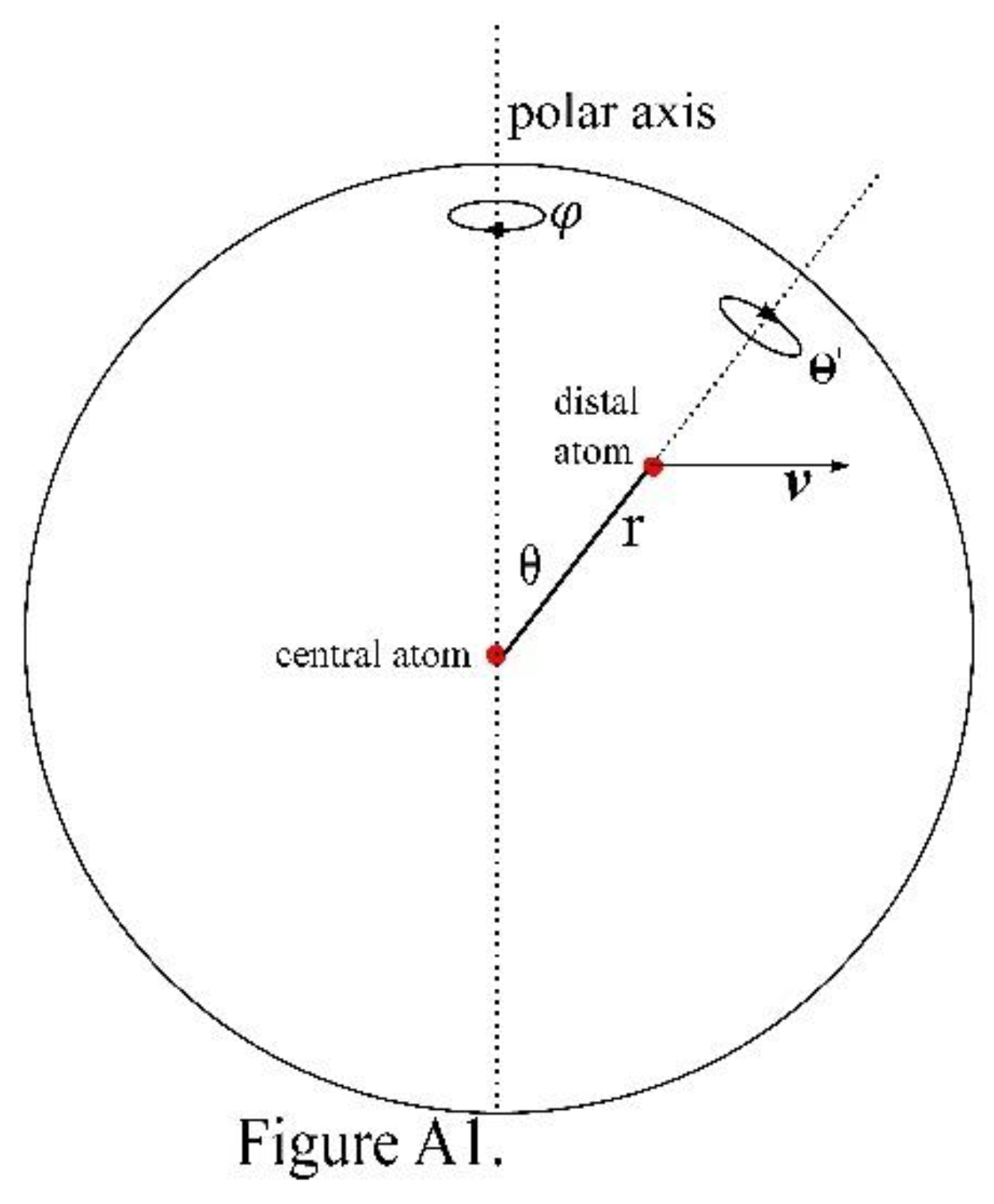
We pop the balloon. The thermal energy Ui is temporarily and partly transformed into (radial) kinetic gain Ek:
Which is the scalar difference between the outward and inward radial components of the atoms’ tensors. For an idle sphere, the inward and outward radials of v in (A3) are equal. We can double (A3)’s inward radial and replace the radial expression in (A2), giving :
Combining (A2), (A3) and (A4) gives:
When idle, . When expanding, .
Since loss to gravity is negligible, for the r2 sphere throughout expansion, which lasts for a second or two. Initially drops and Ek rises. The atoms quickly bounce off the wall and Ek drops back down. At reequilibrium, Ek→0, the terms of (A3) again cancel, and is restored: “”. The gain ΔES from volume increase is:
A1.2. Bound, nonequilibrium free expansion
Take that same balloon, put it in the center of a large vacuum chamber (r2 = 108 m) and pop it. A helium atom at T = 300K has a root mean square speed vrms = 1368 m/s. Those atoms will take about 20 hours to reach the wall if their tensor of movement is perfectly radial. As they expand, they stop colliding with each other at any meaningful rate. After that happens, atomic movement is in an unbound regime which is best considered when the atoms have stopped colliding, but haven’t hit the wall yet. In this regime, the atomic Hubble parameter is simple:
Once the atoms stop colliding, Ek >> at 300K and almost entirely. Eventually the atoms bounce off the wall, , and the regime slowly ends.
A1.3. Unbound, nonequilibrium free expansion
What if there’s no boundary? There’s no equilibrium to be reached, so for a freely expanding gas, only and there’s no . One can approach Universal conditions at the time of last scattering by looking only at the comoving core of a popped sphere with initial rcore = 10-6 rsphere. The atoms in that core would be slow, cold, and nearly isodense (dρ/dr ≈ 0) with a uniform which obeys (11). This sort of treatment could be accurate at scales large enough to include gravity. I’m not suggesting that the Universe has finite mass, only that it can be so modeled.
Appendix B. Initial radial velocity in the adiabatic sphere
We start with the increment radial velocity :
We follow as a function of r, using a fixed increment = 10-9. Below the cutoff radius rc = 0.003 re, loss to gravity is negligible, and all these small spheres have the same value to within 5 ppm (Figure B1):
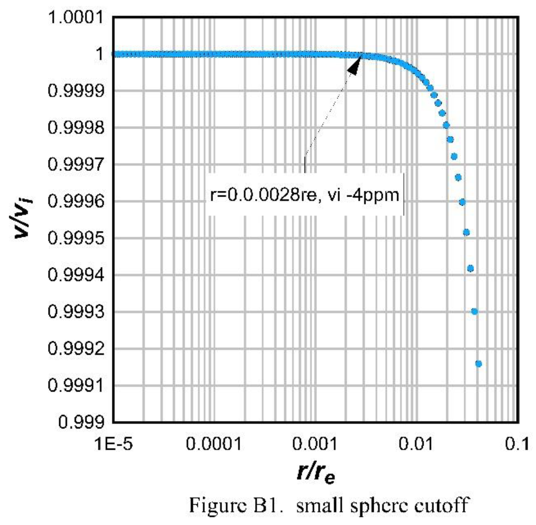
Here we used dE =PdV. Combining (27) and (B1) gives an initial radial velocity vi:
We can determine if energy is conserved within (B2) by examining the partition error (B3):
We increment a small sphere (r1 = 1 x 10¹² m) giving P2 and T2. The pressure drop from thermal loss of our gas is given by:
And the temperature drop by:
Which for (B2) gives a large error. Development in (B1) uses the ideal gas law and not thermal energy. We rearrange (A1):
Substituting for in (B2) gives (29):
By use of (29) the partition error (B3) is only 2 x 10⁻⁸.
Appendix C. Expression of the thermal model in z’
The redshift z2 can be obtained from any starting value z1 by enlarging the increment :
The temperature is found from (B4) and (B5) using (C1) to get V2. Given T(z’=1090) = 2971K, we find from the spreadsheet that is exactly:22
Where the root temperature = 0.002500631 is expressed as degrees K. If treated as an abrupt decoupling at z = 1089, then at z = 60, T = 9.3K; at z = 10, T = 0.3K. These are lower than other estimates [42] but since Hg is temperature-independent, dark thermal heating by the CMB doesn’t affect H. We just need the root temperature.
We insert (C2) into (29), giving:
The endpoint re is adjusted for both T and ρ.
For the T adjustment, the thermal radius change vs. T at constant ρ and Ж is found exactly:
For the ρ adjustment, the thermal radius change vs. ρ at constant T and Ж is found exactly:
For nonrelativistic mass,
Combining these gives:
Inserting (C3) and (C7) into the thermal model (37) gives Newton’s thermal model (C8):
We adjust for relativistic mass with (39):
A linear dependence of H on is found from the spreadsheet, giving the thermal model in Einstein’s Universe (38):
When = 1090, the pure endpoint applies, and we get the pure thermal model (40).
Appendix D. Expression of the suprathermal model in z’
Suprathermal kinetic energy adds entropic pressure to the IGM:
Where and are thermal and suprathermal pressures respectively.
The thermal model (37) has three terms: K, vi, and re. If we want to express suprathermal content within that framework, we need to increase vi or K, decrease re, or some combination. We express vi (29) as a sum:
Where and are thermal and suprathermal kinetic energies in the adiabatic sphere.
The total nucleon kinetic energy Ub is:
Where is the thermal value of Ub, and is cosmic radiation.
The total electron kinetic energy is:
Where is the thermal energy of atomically bound electrons, is the thermal energy of free electrons, and is their suprathermal energy.
Inserting (D3) and (D4) into (D2) gives:
We neglect cosmic radiation for now as its omission doesn’t substantially affect the logic of the following expressions. This means , so:
We examine the thermal energies (bound) and (free). Thermal free electrons are held to behave at very low densities as a monatomic gas. Treatment as such reduces the mean atomic weight Ж. The thermal model is independent of both Ж and T and dependent only on the mean gas density ρg. The result of thermal ionization is thus an increase in both vi and re without affecting H or K. If vi is doubled, so is re, as is the case with pure hydrogen plasma which will serve as our example.
In a thermal system with no ionized H1:
so is reasonably accurate. When H1 is 100% ionized at e.g. 4000K, the number of gas particles is doubled, the atomic weight halved, and energy equipartitioned: , and Ж’ = ½Ж, where Ж’ is the mean atomic weight of the plasma. Making these substitutions into (D6) with no gives:
The added gives twice the old value of vi from (29); more generally, added gives a linear increase in vi and we can expect the same for re. This means that for thermal plasmas, the thermal model (37) is more properly expressed using the nucleon kinetic energy alone:
Where vi and re have their non-ionized values. The denominator term associated with re in (D9) is inserted to comply with the thermal model’s zero-order dependencies. In (D9), vi remains close to (29): Ub ≈ 0.9995Ui, so the effect of thermal ionization on H is minimal, and we can exclude from the thermal model.
We proceed by assuming that suprathermal energy has no effect on either K or re. It may have some effect but we will say it doesn’t. Removal of and from (D6) gives:
When accretion = 0.84 is included we arrive at the suprathermal model (48):
| 1 | Hermann von Helmholtz (1824-1891) is also widely credited. |
| 2 | “Internal energy” was coined by engineers to describe a gas’s thermal energy . Cosmologists added rest energy E=Mc2 to its meaning. |
| 3 | Ludwig Boltzmann (1844-1906). |
| 4 | Isaac Newton (1642-1727). |
| 5 | Euclid of Alexandria (ca. 300 BCE). |
| 6 | “Nucleon” doesn’t include electrons; “Baryon” does. |
| 7 | Pure endpoint values were found from (24) for H0 = 67.00-76.00; = 10(18.8169537022-0.9999999H0); correlation =1. |
| 8 | Most calculations used 997 steps of linearly increasing r/re, beginning at rc/re and ending with r/re = 0.999999 or 1 at step 997. Derived K values at a 997-point refinement were invariant to 5 decimal places. A 9970-point plot gave K = 0.792104 (9969 steps) and 0.792094 (9970 steps); the value ve/vi = K = 0.79210 was selected. |
| 9 | A 9,970-point plot of y (vs/vi)2 vs. x (r/re) when numerically integrated gave a curve with third-order coefficients x0 = -0.00299999, x = 1.0000000, x2 = -1.5 x 10⁻⁹, and x3 = -0.33333333. Correlation = 1. When cutoff x = 0.003 is added to x0, y = 2/3 @ x = 1. |
| 10 | |
| 11 |
=0.002500631. This is the root temperature for a last-scatter 2971K. It’s derived in appendix C. |
| 12 | Alexander Friedmann (1888-1925). |
| 13 | Arthur Compton (1892-1962). |
| 14 |
T = 4,000-50,000K gave the same results for all z. |
| 15 | For the ln-ln regression of H(z) from z = 0 to 2, 101 data points were used with 3+ significant figures for all calculated . Found: y = 0.80455-2.99154x; Correlation 0.9999996; std. error 0.0007. The y intercept gives z = 0.30852. |
| 16 | Found for ln-ln: y = 0.00006 - 1.500563x; correlation 0.99999999. The endpoint is temperature-dependent so a constant T must be used. |
| 17 | Mass loss from nuclear fusion is neglected here, but its added kinetic energy isn’t enough to account for Λ. |
| 18 | Neutrinos are believed to have had relativistic kinetic energy at last scatter but became nonrelativistic in the dark age. This affects their temporal mass density dependence, which is untreated in the present paper. |
| 19 | Max Planck (1858-1947). |
| 20 | An alternate treatment of photon entropy using J/K instead of J/Hz is given by Kirwan [43]. |
| 21 | This paper is deposited with Physical Review D; code number DN13643. |
| 22 | 210 points from z’ = 1090 to 10; median z’ = 350. Found: T = 2 x 10⁻⁹ + 5 x 10-11(z’) + 0.002500631 (z’)2; correlation = 1. |
References
- A. A. Penzias & R. W. Wilson. “A measurement of excess antenna temperature at 4080 Mc/s”. Astrophys. J. 142, 419-421 (1965), https://adsabs.harvard.edu/full/1965ApJ...142..419P/0000419.000.html.
- C. O’Raifeartaigh, M. O’Keeffe, W. Nahm, & S. Mitton. “Einstein’s 1917 static model of the universe: a centennial review”, Eur. Phys. J. H 42, 431-474 (2017). [CrossRef]
- E. Hubble, “A relation between distance and radial velocity among extra-galactic nebulae”, Proc. Nat. Acad. Sci. 15, 3, 168-173 (1929) . [CrossRef]
- S. Perlmutter et al., Discovery of a supernova explosion at half the age of the Universe. Nature 391, 51-54 (1998) . [CrossRef]
- S. Perlmutter et al., “Measurements of Ω and Λ from 42 high-redshift supernovae”, Astrophys. J. 517, 2, 565-586 (1999) . [CrossRef]
- A. G. Riess et al., “Observational evidence from supernovae for an accelerating Universe and a cosmological constant” Astron. J. 116, 3, 1009 (1998) . [CrossRef]
- A. G. Riess et al., “Type Ia supernova discoveries at z > 1 from the Hubble space telescope: Evidence for past deceleration and constraints on dark energy evolution”, Astrophys. J. 607, 2, 665 (2004) . [CrossRef]
- P. Bull et al. “Beyond ΛCDM: Problems, solutions, and the road ahead”. Phys. Dark. Univ. 12, 56-99 (2016), . [CrossRef]
- Planck Collaboration, “Planck 2018 results” A&A 641, A1 (2020) . [CrossRef]
- A. G. Riess et al., “New parallaxes of galactic cepheids from spatially scanning the Hubble space telescope: Implications for the Hubble constant”, Astrophys. J. 855, 136 (2018) . [CrossRef]
- A. G. Riess, S. Casertano, W. Yuan, L. M. Macri, & D. Scolnic, “Large Magellanic cloud cepheid standards provide a 1% foundation for the determination of the Hubble constant and stronger evidence for physics beyond ΛCDM”, Astrophys. J. 876, 85 (2019) . [CrossRef]
- L. Verde, T. Treu, and A. G. Riess, “Tensions between the early and late Universe”, Nat. Astron. 3, 891-895 (2019) . [CrossRef]
- A. J. Shajib et al, “STRIDES: a 3.9 per cent measurement of the Hubble constant from the strong lens system DES J0408−5354”, MNRAS 494, 6072-6102 (2020) . [CrossRef]
- K. C. Wong et al., “H0LiCOW – XIII. A 2.4 per cent measurement of H0 from lensed quasars: 5.3σ tension between early- and late-Universe probes”. MNRAS 498, 1420-1439 (2020) . [CrossRef]
- D. Scolnic et al. “Systematic uncertainties associated with the cosmological analysis of the first pan-starrs1 type 1a supernova sample”, Astrophys. J. 795, 45 (2014). [CrossRef]
- V. Poulin, T. L. Smith, T. Karwal and M. Kamionkowski, “Early dark energy can resolve the Hubble tension”, Phys. Rev. Lett. 122, 221301 (2019) . [CrossRef]
- N. Schӧneberg, J. Lesgourges, and D. C. Hooper, “The BAO+BBN take on the Hubble tension”, J. Cosmol. Astroparticle Phys. 2019, 10, 029 (2019) . [CrossRef]
- C. L. Steinhardt, A. Sneppen, and B. Sen, “Effects of supernova redshift uncertainties on the determination of cosmological parameters”, Astrophys. J. 902, 14 (2020) . [CrossRef]
- G. Alestas and L. Perivolaropoulos, “Late-time approaches to the Hubble tension deforming H(z), worsen the growth tension”, MNRAS 504, 3956-3962 (2021) . [CrossRef]
- E. Di Valentino et al., “In the realm of the Hubble tension - a review of solutions”, Classical and Quantum Gravity 38, 153001 (2021) . [CrossRef]
- C. Krishnan, E. Ó Colgáin, M. M. Sheikh-Jabbari and T. Yang, “Running Hubble tension and a H0 diagnostic”, Phys. Rev. D 103, 10, 103509 (2021) . [CrossRef]
- M. Rameez and S. Sarkar, “Is there really a Hubble tension?”, Classical and Quantum Gravity 38, 154005 (2021) . [CrossRef]
- D. Aloni, A. Berlin, M. Joseph, M. Schmaltz and N Weiner, “A Step in understanding the Hubble tension”, Phys. Rev. D. 105, 12, 123516 (2022) . [CrossRef]
- L. Perivolaropoulos & F. Skara, “Challenges for ΛCDM: An update”, New Astron. Rev. 95, 101659 (2022) . [CrossRef]
- N. Mostaghel, “The source of tension in the measurements of the Hubble constant”, Int. J. Astron. Astrophys. 12, 3, 273-280 (2022) . [CrossRef]
- V. Netchitailo, “Hubble tension”, JHEPGC 8, 2, 392-401 (2022) . [CrossRef]
- S. Tsujikawa, “Quintessence: a review”, Classical and Quantum Gravity 30, 214003 (2013) . [CrossRef]
- P. W. Higgs, “Spontaneous Symmetry Breakdown without Massless Bosons”, Phys. Rev. 145, 1, 156-1163 (1966) . [CrossRef]
- E. Verlinde, “On the origin of gravity and the laws of Newton”, J. High Energy Phys. 4, 20 (2011) . [CrossRef]
- S. Weinberg, The First Three Minutes, Basic Books Press (1988).
- J. M. Owen and J. V. Villumsen, “Baryons, dark matter, and the Jeans mass in simulations of cosmological structure formation”, Astrophys. J. 481, 1, 1-21 (1997) . [CrossRef]
- J. Miralda-Escude, “The dark age of the Universe”, Science 300, 5267, 1904-1909 (2003) . [CrossRef]
- A. Natarajan and N. Yoshida, “The dark ages of the Universe and hydrogen reionization”, Prog. Theor. Exp. Phys. 2014, 06B112 (2014) . [CrossRef]
- G. Bertone and D. Hooper, “History of dark matter”, Rev. Mod. Phys. 90, 045002 (2018) . [CrossRef]
- B. E. Robertson et al., “Identification and properties of intense star-forming galaxies at redshifts z>10”, Nat. Astron. 7, 5, 611-621 (2023) . [CrossRef]
- E. Curtis-Lake et al., “Spectroscopic confirmation of four metal-poor galaxies at z = 10.3–13.2”, Nat. Astron. 7, 5, 622-632 (2023) . [CrossRef]
- H. Yüksel, M. D. Kistler, J. F. Beacom, and A. M. Hopkins, “Revealing the high-redshift star formation rate with gamma-ray bursts”, Astrophys. J. 683, 1, L5 (2008) . [CrossRef]
- D. Wanderman and T. Piran, “The luminosity function and the rate of Swift's gamma-ray bursts”, MNRAS 406, 3, 1944-1958 (2010) . [CrossRef]
- A. Liddle, An introduction to modern cosmology, Wiley. ISBN 978-1-118-50214-3 (2015).
- B. Ryden, Introduction to cosmology, second edition. Cambridge University Press (2017) https://www.cambridge.org/9781107154834.
- C. O’Raifeartaigh and S. Mitton, “Interrogating the Legend of Einstein's ‘Biggest Blunder’”, Physics in Perspective 20, 4, 318-321 (2018) . [CrossRef]
- T. Venumadhav, L. Dai, A. Kaurov and M. Zaldarriaga, “Heating of the intergalactic medium by the cosmic microwave background during cosmic dawn”, Phys. Rev. D 98, 10, 103513 (2018) . [CrossRef]
- A. D. Kirwan Jr., “Intrinsic photon entropy? The darkside of light”, Int. J. Eng. Sci. 42, 7, 725-734 (2004) . [CrossRef]

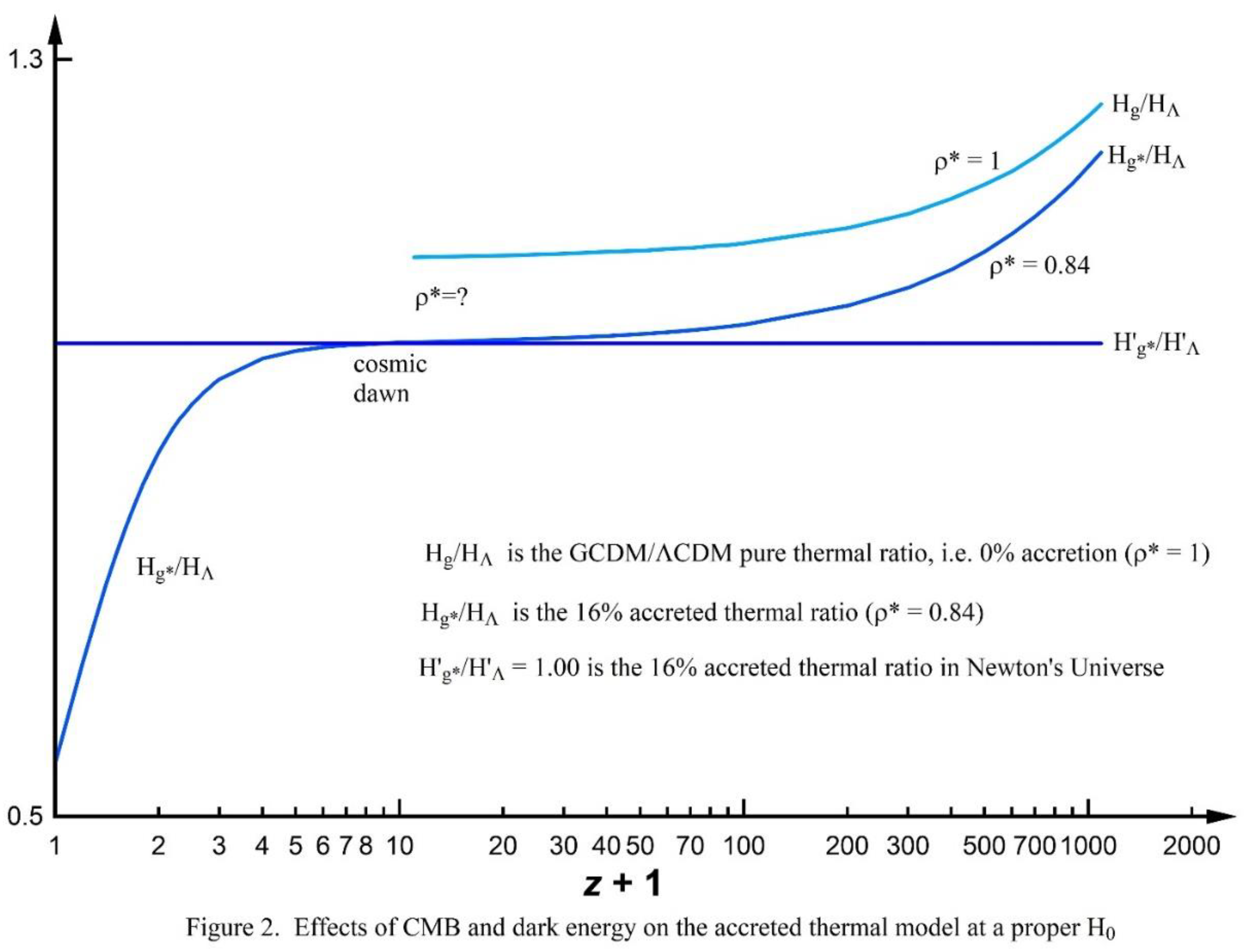
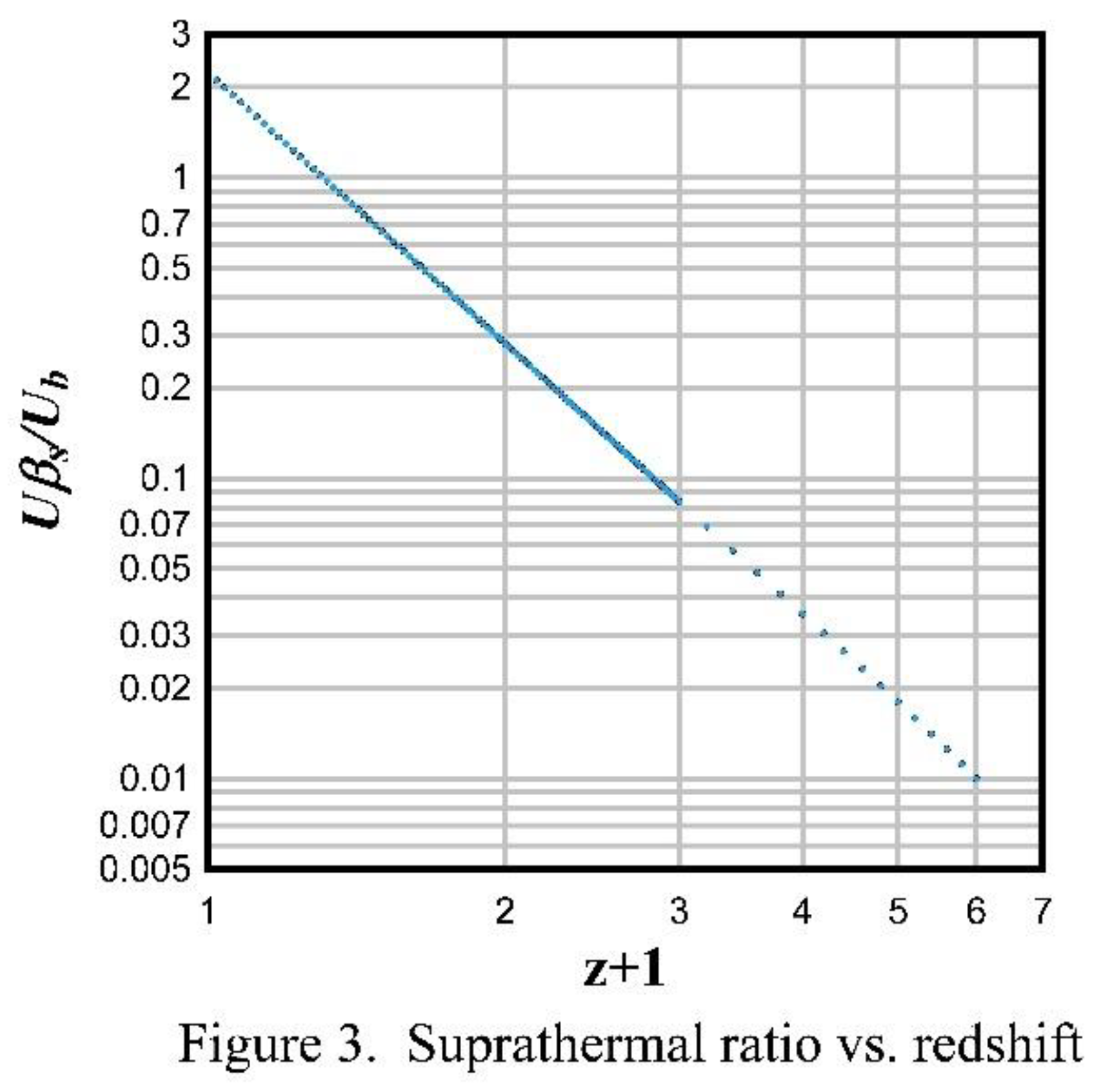

Table 1.
Values at z = 0.
| H0 | 67.70 km/sec/Mpc |
| H0 | 2.1938 x 10⁻¹⁸ sec-1 |
| ρcrit | 8.6075 x 10⁻²⁷ kg/m3 |
| Baryons Ωb | 0.04898 |
| Cold dark matter Ωc | 0.26104 |
| Relativistic energy Ωλ | 0.000091 |
| Dark energy ΩΛ | 0.6908 |
| TCMB | 2.6270 K |
| Note: H0 and the Ω’s were calculated from table 6 of [9], except ΩΛ = 1- (Ωb+Ωc+Ωλ). | |
Table 2.
The effect of relativistic (CMB) energy on the Hubble parameter.
| z = 0 | z = 1089 | |||||
| H0 | H0 | Hg | HΛ | Hg/H0 | HΛ/H0 | Hg/HΛ |
| (km/sec/Mpc) | (sec-1) | (sec-1) | (sec-1) | |||
| BOTH GCDM AND ΛCDM CONTAIN CMB ENERGY (Einstein’s Universe) | ||||||
| 67.70 | 2.194 x 10⁻¹⁸ | 6.319 x 10⁻¹⁴ | 5.045 x 10⁻¹⁴ | 28,805 | 22,995 | 1.253 |
| 74.40 | 2.411 x 10⁻¹⁸ | 6.945 x 10⁻¹⁴ | 5.544 x 10⁻¹⁴ | 28,805 | 22,995 | 1.253 |
| GCDM DOES NOT CONTAIN CMB ENERGY, ΛCDM DOES | ||||||
| 67.70 | 2.194 x 10⁻¹⁸ | 4.784 x 10⁻¹⁴ | 5.045 x 10⁻¹⁴ | 21,807 | 22,995 | 0.948 |
| 74.40 | 2.411 x 10⁻¹⁸ | 5.257 x 10⁻¹⁴ | 5.544 x 10⁻¹⁴ | 21,807 | 22,995 | 0.948 |
| NEITHER GCDM NOR ΛCDM CONTAIN CMB ENERGY (Newton’s Universe) | ||||||
| 67.70 | 2.194 x 10⁻¹⁸ | 4.784 x 10⁻¹⁴ | 4.389 x 10⁻¹⁴ | 21,807 | 20,008 | 1.090 |
| 74.40 | 2.411 x 10⁻¹⁸ | 5.257 x 10⁻¹⁴ | 4.824 x 10⁻¹⁴ | 21,807 | 20,008 | 1.090 |
| NEITHER ΛCDM NOR GCDM CONTAIN CMB ENERGY, AND GCDM’S GAS DENSITY IS REDUCED BY 15.8%: ρg = 0.8418 ρb | ||||||
| 67.70 | 2.194 x 10⁻¹⁸ | 4.389 x 10⁻¹⁴ | 4.389 x 10⁻¹⁴ | 20,008 | 20,008 | 1.000 |
| 74.40 | 2.411 x 10⁻¹⁸ | 4.824 x 10⁻¹⁴ | 4.824 x 10⁻¹⁴ | 20,008 | 20,008 | 1.000 |
Disclaimer/Publisher’s Note: The statements, opinions and data contained in all publications are solely those of the individual author(s) and contributor(s) and not of MDPI and/or the editor(s). MDPI and/or the editor(s) disclaim responsibility for any injury to people or property resulting from any ideas, methods, instructions or products referred to in the content. |
© 2024 by the authors. Licensee MDPI, Basel, Switzerland. This article is an open access article distributed under the terms and conditions of the Creative Commons Attribution (CC BY) license (http://creativecommons.org/licenses/by/4.0/).
Copyright: This open access article is published under a Creative Commons CC BY 4.0 license, which permit the free download, distribution, and reuse, provided that the author and preprint are cited in any reuse.