1. Introduction
Remarkable progress has been made in the development of methods and tools for modeling and simulating the production, processing, and structural properties of steels and metal alloys. Computational modeling, a cost-effective approach to optimize factors such as chemical composition and process conditions, is widely used in scientific and industrial research and helps to achieve the desired properties of metal materials [
1,
2,
3,
4].
A more cost-effective approach for evaluating the hardness of continuously cooled steel from the austenitizing temperature is the Jominy end-quench test. Integrating the results of this test into models used for heat treatment simulations requires the computation of cooling rates at specific locations on the cooled object, associating them with respective distances from the quenched end of the sample [
5]. The techniques for computing Jominy hardenability curves are described in detail in various studies, including [
6,
7,
8,
9,
10,
11].
Modern steelmaking techniques allow precise regulation of chemical composition and hardenability, with some manufacturers advocating strict limitations on hardenability. The widely used Jominy end quench hardenability test is an important tool in the production, specification, procurement, and application of heat-treatable structural steels, which are critical to modern transportation, construction, and agricultural machinery. The delineation of hardenability bands and the associated metallurgical methods, which link hardenability to heat treatment response, microstructure evolution, and eventual mechanical properties, form the basis for the economically viable selection of steels and the design of components [
12].
The hardenability of steel depends on its composition, subject to specific limits defined for each steel grade. Despite compliance with the compositional specifications, a typical variation in hardenability can occur for each steel grade. In certain cases, tighter compositional control is essential for the applications for which the steel is used. Therefore, several steels are offered in H-grade variants that have tighter compositional control. The extent of control is precisely defined by the maximum and minimum hardenability limits [
13].
In the field of materials engineering, there is growing interest in the use of artificial and computational intelligence [
4,
14,
15]. The increasing accessibility of material databases and advances in machine learning open up new possibilities for the prediction of material properties and the development of next-generation materials [
16,
17,
18,
19]. One of the best-known methods of computational intelligence is the use of artificial neural networks (ANN) [
20,
21,
22]. Artificial neural networks (ANNs) are invaluable for practical applications as they overcome the hurdles associated with formulating mathematical models. Their ability to establish connections between studied variables without the need for explicit mathematical descriptions is a distinctive feature that enables ANNs to learn solutions to problems based on identified patterns from the given experimentally collected data [
1,
23,
24,
25].
Artificial neural networks (ANNs), especially multilayer perceptron networks (MLPs), are widely used in modeling steel and metal alloy problems due to their efficiency in handling classification and regression tasks. ANNs are characterized by their ability to learn from labeled data sets and are therefore well suited for supervised learning applications [
26,
27,
28]. The key requirement for the development of an effective neural model is the creation of a representative data set. To do this, the value range of the variables must be determined, and their statistical distribution evaluated. Proper training of the neural network requires the representation of patterns that evenly cover the entire range of variables. The analysis emphasizes the importance of precisely defining the range of independent variables for neural models to avoid errors when extrapolating beyond the range of the training data, especially in multidimensional input domains. Selecting the optimal number of neurons in the hidden layer of an MLP network is about finding a balance between approximation and generalization, with overfitting being a well-studied problem. There are different approaches to determine the optimal number of neurons, often favoring the lowest error value, although the arbitrary application of this criterion may increase the risk of overfitting. The evaluation of neural models relies heavily on a comprehensive test set that adequately represents the full range of the model. Statistical values for the test set, such as the mean absolute error and the correlation coefficient, should match those of the training set and thus provide a crucial insight into the quality of the model [
1,
29].
Splitting a dataset into different subsets for training and validation is a fundamental aspect of machine learning and plays a crucial role in various tasks such as model evaluation, model comparison, and hyperparameter tuning. Common methods such as holdout, bootstrap, and cross-validation (CV) are often used for this purpose [
30]. In this method, the available data set is divided into two different subsets: a training set, which is used to determine the model parameters, and a separate validation set (test set), also known as the hold-out set or development set. The training set is crucial for model parameterization, while the validation set serves as an independent data set for evaluating the performance of the model. The selection criterion for the final model is to select the one that has the least error in the validation set. This approach ensures that the selected model generalizes well to new, unseen data [
24].
Cross-validation (CV) is a well-known resampling method that is widely used in statistical learning methods. It serves as an important tool for estimating the test error associated with a particular statistical learning method and makes an important contribution to model evaluation and selection. Evaluating the overall performance of a model and selecting an appropriate degree of flexibility are integral aspects of cross-validation that are essential for refining and optimizing statistical learning models [
31].
The selection of k in k-fold cross-validation involves a trade-off between bias and variance. The parameter k determines the number of folds into which the data set is divided and influences the estimation of the model’s test error. It is common to use k = 5 or k = 10, as empirical evidence suggests that these values lead to a balance yielding test error rate estimates with moderate bias and variance. This choice helps to reduce the risk of underfitting (high bias) or overfitting (high variance) in the model evaluation process [
31]. Furthermore, a comparison between 5-fold cross-validation and 10-fold cross-validation shows that 10-fold cross-validation generally performs better in regression scenarios [
32].
Bayesian optimization (BO), known for its efficiency in optimizing expensive black-box functions, has attracted considerable attention, especially in the field of hyperparameter optimization. The basic concept involves approximating the unknown function, typically using Gaussian processes, with initial random estimates and iterative updates with each new observation. Success in navigating a multidimensional space with numerous hyperparameters depends on an appropriate number of iterations and careful selection of hyperparameter ranges, which are influenced by factors such as the size of the data set, expert judgment, intuition, and computational resources. Since most machine learning algorithms require the configuration of a range of hyperparameters, the careful selection of their values has a significant impact on performance. To streamline the time-consuming and non-reproducible manual trial-and-error process of determining the optimal hyperparameter configurations, automatic hyperparameter optimization through Bayesian optimization can be used [
33,
34].
With limited datasets, BO proves to be more advantageous than grid search for tuning hyperparameters. The effectiveness of BO results from the use of a probabilistic model, which enables a more efficient search for optimal hyperparameters at a lower computational cost. Bayesian tuning of hyperparameters is excellent for exploring the hyperparameter space and strengthening the robustness of machine learning models, especially in scenarios with small datasets. Initially, the BO approach searches for the initial set of hyperparameters through various combinations, guided by considerations of the problem space and presumptions about the potential impact of the model hyperparameters. After determining the initial hyperparameters, BO employs a probabilistic model to construct a surrogate model that facilitates the estimation of model performance in a large hyperparameter space. The model is then trained with the initial set of hyperparameters. This iterative process of model training and evaluation with different hyperparameters allows BO to accumulate more data points and thus improve the performance and accuracy of the surrogate model. As the surrogate model evolves, the algorithm becomes more adept at making informed decisions about where to look for the best hyperparameters. This iterative refinement process proves invaluable in identifying optimal hyperparameters within limited data sets, leading to improved model performance [
35,
36,
37].
During the execution of an experiment, the Experiment Manager actively searches for the optimal combination of hyperparameters. Using a trial-and-error approach, a new set of hyperparameters is tested at each iteration of the experiment, considering the results of the previous experiments. Bayesian optimization plays a central role in this process by gradually building a probabilistic model of the objective function. This iterative method guides the selection of subsequent sets of hyperparameters, continuously refining the model’s estimate of the function’s behavior. Ultimately, this iterative strategy facilitates the identification of the most advantageous hyperparameter configuration for a machine learning model.
2. Materials and Methods
Feed-forward neural networks, a subtype of artificial neural networks, are used for modeling classification and regression problems. A two-layer feed-forward network, often referred to as a shallow neural network, consists of an input layer, a hidden layer, and an output layer. In this architecture, the input layer receives data and the hidden layer utilizing an activation function, applies weights and biases to the inputs. The final output is generated by the output layer. The hidden layer is critical for capturing complex patterns in the data and the network refines its understanding by adjusting the weights and biases during the training process. Despite their relative simplicity compared to deeper architectures, two-layer feed-forward networks can prove effective for certain problems, especially when dealing with less complex data or limited computational resources.
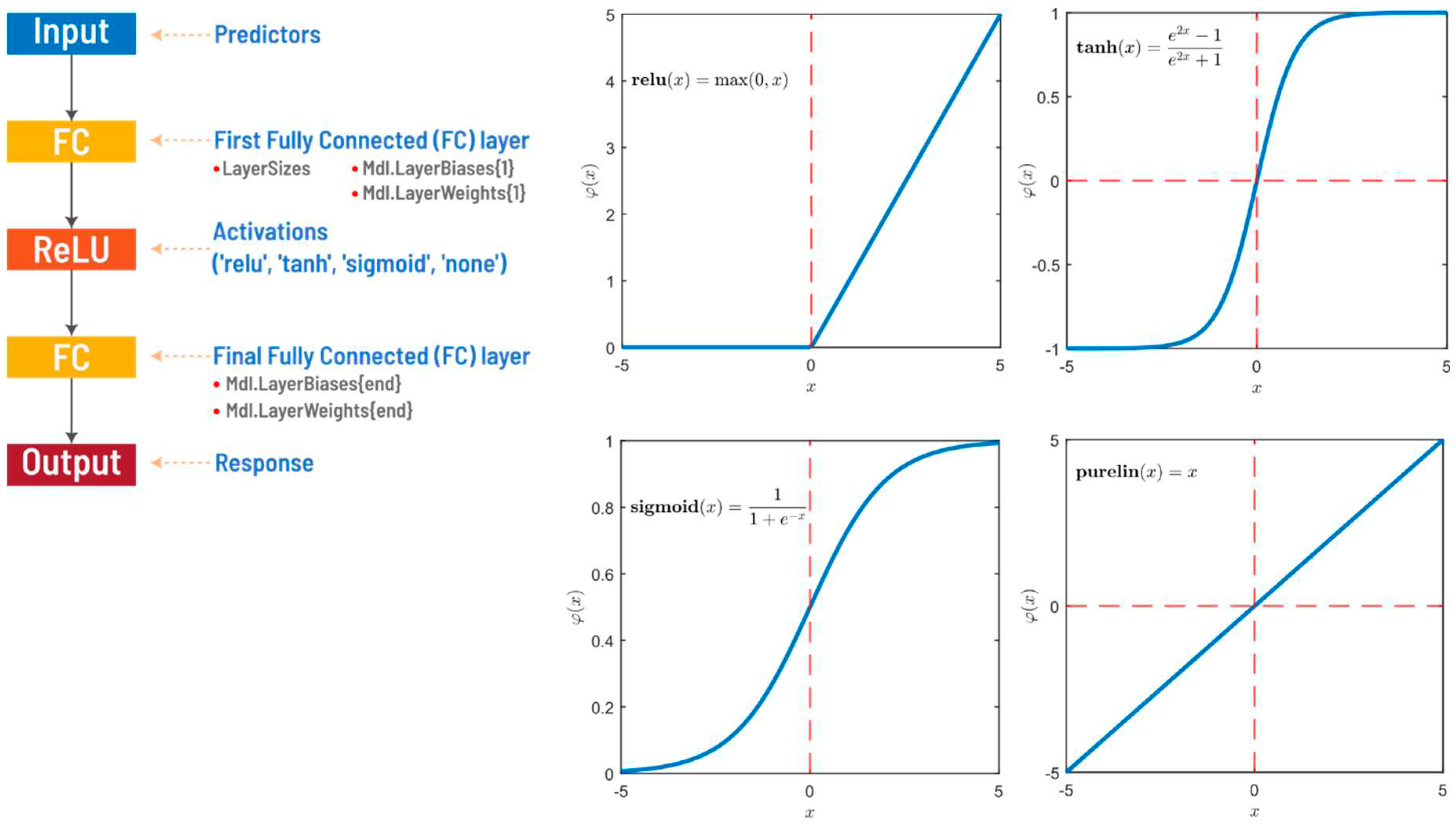
A RegressionNeuralNetwork object is a trained, feedforward and fully connected neural network for regression. The first fully connected layer of the neural network has a connection from the network input (predictors) and each subsequent layer has a connection from the previous layer. Each fully connected layer multiplies the input by a weight matrix (LayerWeights) and then adds a bias vector (LayerBiases). An activation function follows each fully connected layer, except for the last layer (Activations and OutputLayerActivation). The last fully connected layer generates the output of the network, namely the predicted response values. The solver utilized for training the neural network model is referred to as ’LBFGS". In the context of creating the RegressionNeuralNetwork model, fitrnet employs the limited-memory Broyden-Fletcher-Goldfarb-Shanno quasi-Newton algorithm (LBFGS) as an optimization algorithm to minimize the loss function. Specifically, the software aims to minimize the mean squared error (MSE) during the training process.
Figure 1.
Typical feed-forward, fully connected neural networks for regression [
38] (
left) and activation functions used in the modeling task (
right).
Figure 1.
Typical feed-forward, fully connected neural networks for regression [
38] (
left) and activation functions used in the modeling task (
right).
Bayesian optimization is an iterative algorithm with a probabilistic surrogate model and an acquisition function to select the next evaluation point. Each iteration involves fitting the surrogate model to all past observations of the objective function. The acquisition function uses the predictive distribution of the probabilistic model to guide the selection of candidate points and balance exploration and exploitation. This approach, which is less costly than directly evaluating the expensive black box function, allows for comprehensive optimization of the acquisition function. Although various acquisition functions are available, the expected improvement (EI) is often preferred because it can be calculated analytically if the model prediction y for the configuration λ follows a normal distribution, Equations (1) and (2) [
39,
40,
41].
here,
and
denote the standard normal density and standard normal distribution function, respectively, and
represents the best observed value thus far.
When searching for optimal values for the regression hyperparameters, MATLAB offers various optimization techniques, including Bayesopt, grid search, and random search, with Bayesian optimization (bayesopt) being the default setting. When selecting the hyperparameters for the subsequent experiment, any of the acquisition functions can be used, such as expected improvement per second plus, expected improvement, expected improvement plus, expected improvement per second, lower confidence bound, or probability of improvement, as optimization option.
There are many alternative CV schemes, of which k-fold CV is one of the most popular. The k-fold CV is a widely used resampling method in the practical application of statistical learning methods. The set of observations is randomly divided into k groups (folds) of approximately equal size. In each iteration, the first fold is designated as the validation set and the model is trained on the remaining k−1 folds. The mean square error (MSE) is then calculated for the observations in the remaining group. This process is repeated k times, resulting in k estimates of the test error (MSE
1, MSE
2,..., MSE
k). The final k-fold CV estimate is obtained by averaging these values, Equation (3) [
31]:
Finally, the observations of the test set are used as an independent data set to evaluate the performance of the model and select the model. The model with the smallest test RMSE and the smallest mean absolute error (MAE) is selected as the final model, as these metrics ensure that the selected model generalizes well to a new data set. In addition to RMSE, mean square error (MSE), mean absolute error (MAE), and coefficient of determination (R
2) are used to evaluate the model during the test performance analysis, Equations (4)-(7).
where n is the total number of experimental observations,
is the experimental values for each of the runs,
is the predicted value for each of the observed values, and
is the mean of the experimental values of the runs.
We assessed the cross-validation loss of neural network regression models by examining various hyperparameter settings, including regularization strengths (lambda), activation functions (’relu’, ’tanh’, ’sigmoid’, ’none’), hidden layer sizes, and hidden node sizes. We then fine-tuned the hyperparameters using Bayesian optimization to find the optimal configuration that minimizes model error and improves performance.
2.1. Analysis of the Dataset
The data set contains data on measurements on the Rockwell Hardness scale C at distances of 1.5, 3, 5, 7, 9, 11, 13, 15, 20, 25, 30, 40 and 50 mm. It also contains information on the percentage of mass fraction of concentration of the seven basic alloying elements found in the group of alloyed structural alloy steel, namely C, Mn, Si, Cr, Ni, Mo, and Cu.
Table 1 outlines the ranges of predictors and response parameters used in modeling the hardenability of steels.
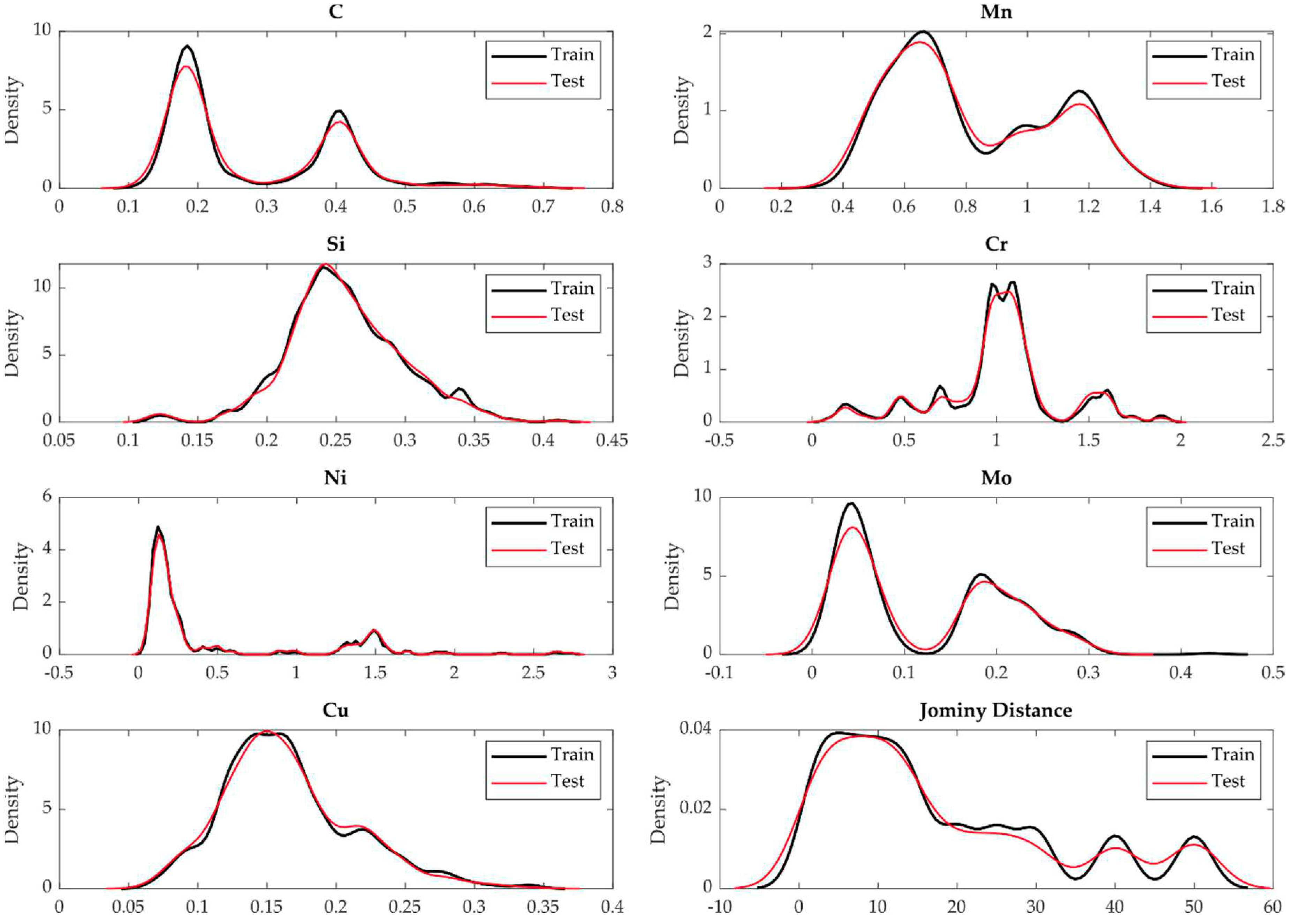
The goal of predictive hardenability modeling is to create a model based on the training dataset and then apply this model to the test dataset. However, to achieve the best results, the training dataset must be a representative sample of the data we want to apply it to (i.e. the test dataset). Otherwise, our model will be inadequate at best or completely useless at worst. The Kolmogorov-Smirnov test checks whether the distributions of the two samples (training and test data sets) differ significantly from each other. The null hypothesis is that the samples come from the same distribution [
42].
Table 2 presents the results of the Kolmogorov-Smirnov test, which is used to assess the goodness of fit of the training and test data sets.
To assess the similarity of the feature distributions between the training and test datasets, we performed Kolmogorov-Smirnov (KS) tests at a 5% significance level for each feature. The KS test values, which represent the maximum absolute differences between the cumulative distribution functions, were calculated for the features C, Mn, Si, Cr, Ni, Mo, Cu, Jominy distance, and hardness (HRC). The KS test values obtained are between 0.020 and 0.033, indicating relatively small differences between the distributions. In addition, p-values were calculated for each test, ranging from 0.37 to 0.91. Significantly, all calculated p-values were relatively high, indicating that there is no substantial evidence to reject the null hypothesis of similarity between the distributions. These results provide confidence in the similarity of the feature distributions between the training and test datasets and confirm the robustness of our partitioning of the datasets for training and evaluating the models, i.e. the model is likely to generalize well to the unseen test dataset.
Figure 2.
Training and test data sets splits distribution.
Figure 2.
Training and test data sets splits distribution.
Five distinct experiments with different hyperparameter settings were conducted for the hyperparameter optimization process. The experiments were run for 1500 trials and validation RMSE was recorded as the performance metric.
Experiment 1 (10-fold CV): NumLayers [1, 2], Activations [‘relu’, ‘tanh’, ‘sigmoid’, ‘none’], Standardize [‘true’, ‘false’], lambda [1.9172e-09, 0.1], Layer 1 [1, 300] and Layer 2 [1, 300].
Experiment 2 (5-fold CV): NumLayers [1, 2], Activations [‘relu’, ‘tanh’, ‘sigmoid’, ‘none’], Standardize [‘true’, ‘false’], lambda [1.9172e-09, 0.1], Layer 1 [1, 300] and Layer 2 [1, 300].
Experiment 3 (10-fold CV): Layer 1 [1, 300], Activations [‘relu’, ‘tanh’, ‘sigmoid’, ‘none’], Standardize [‘true’, ‘false’] and lambda [1.9172e-09, 0.1].
Experiment 4 (10-fold CV): Layer 1 [1, 100], Activations [‘relu’, ‘tanh’, ‘sigmoid’], Standardize [‘true’, ‘false’] and lambda [1.9172e-09, 0.1].
Experiment 5 (10-fold CV): Layer 1 [1, 30], Activations [‘relu’, ‘tanh’, ‘sigmoid’], Standardize [‘true’, ‘false’] and lambda [1.9172e-09, 0.1].
For the tuning of hyperparameter process 5-fold and 10-fold CV were employed to protect the model against overfitting. Experiment 1 and Experiment 2 have the same hyperparameter settings with different cross-validation folds.
In this study, the main data set of 6136 observations is randomly split into two sets: A training dataset contains 85% of the observations used to determine the model parameters and hyperparameters, and a separate model test set contains the remaining 15% of the observations. The training dataset is then used for k-fold cross-validation during the training and validation phase of model development. The training dataset containing the observations is randomly split into k mutually exclusive folds of approximately equal size. In each iteration, the first fold is determined as the validation set, and the model is trained on the remaining k−1 folds. The root mean square error (RMSE) is then calculated for the observations in the remaining fold. This process is repeated k times, resulting in k estimates of the validation error. The average of these results is the final estimate of the k-fold CV and is reported as the validation RMSE of the model.
3. Results
This section provides a comprehensive overview of model training and tuning, performance analysis, and model evaluation and selection to obtain the best-performing model for prediction and deployment. The performance of the various neural network configurations was evaluated using the root mean square error (RMSE) and the configuration with the lowest RMSE was selected for subsequent model testing using a separate test dataset. The tuned models were thoroughly evaluated to determine the most appropriate configuration for accurate hardness prediction. All models use standardized data sets and the sigmoid activation function that appears to be effective for the modeling task.
3.1. Experimental Results Analysis
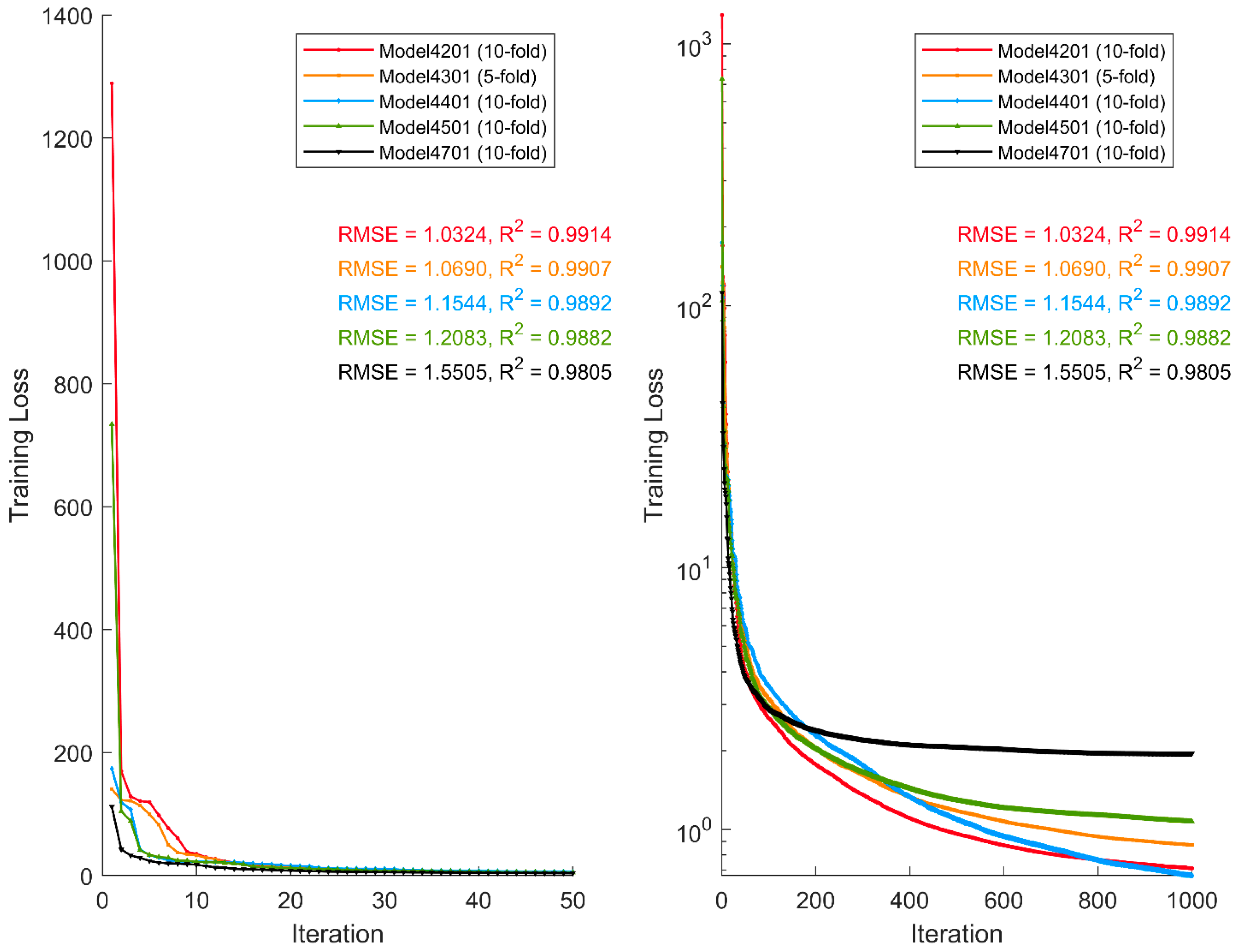
Table 3 presents five optimal models determined by Bayesian optimization of the hyperparameters in five different experiments, and their performance evaluations. These results indicate the performance of each model. The RMSE and R
2 values for both the training and test
datasets show how well the models generalize to unseen data set.
All models perform well, as shown by the relatively low RMSE values for both the training and test datasets. The R2 values, which represent the proportion of variance explained, are consistently high, indicating that the models capture a significant portion of the variability in the data.
Model II is characterized by the lowest RMSE in the test data set (1.0976), indicating a higher predictive accuracy compared to the other models. Model V has shown the highest RMSE on the test data set (1.6299), indicating that it is less effective when generalizing to new data.
The differences in architecture (number of hidden layers and nodes) between the models do not consistently correlate with performance. Models I, III, IV and V show similar performance values despite their different architectures. The lambda values for regularization vary, indicating the influence of regularization strength on model performance.
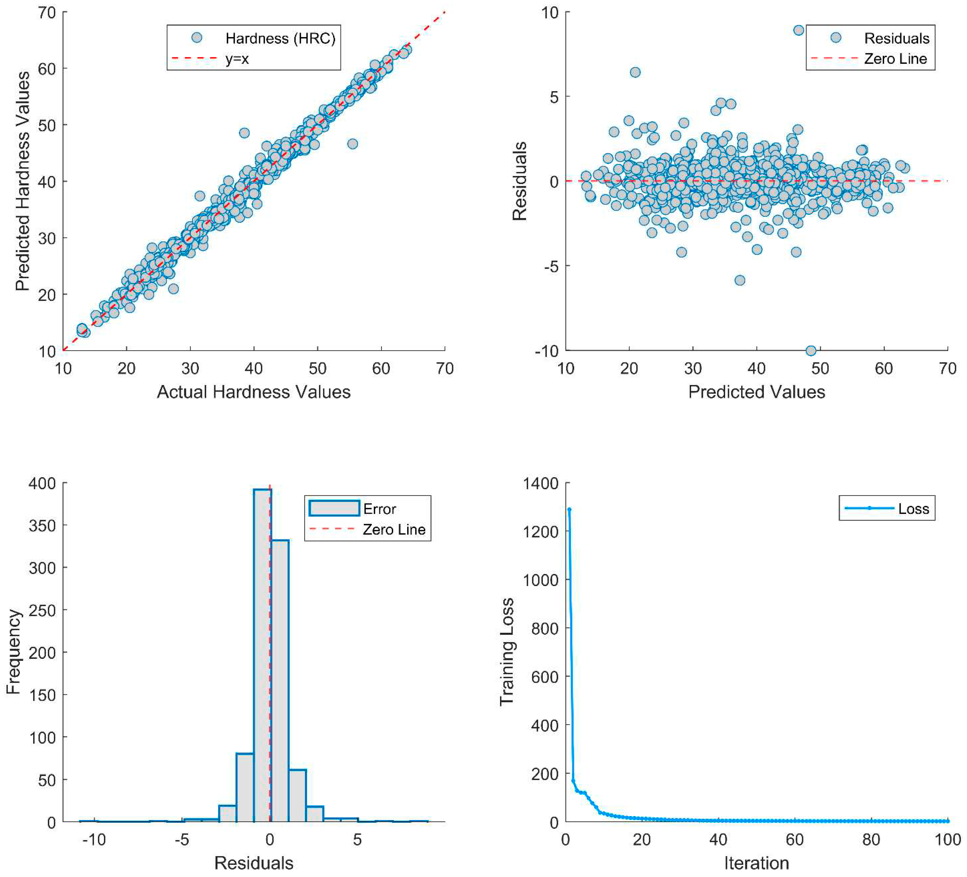
Of the top models from each experiment, Model II proves to be the most promising, as it has the lowest RMSE for the test set and high R2 values. It appears to be the best-performing model among the options offered and shows superior predictive accuracy for the new unseen test set.
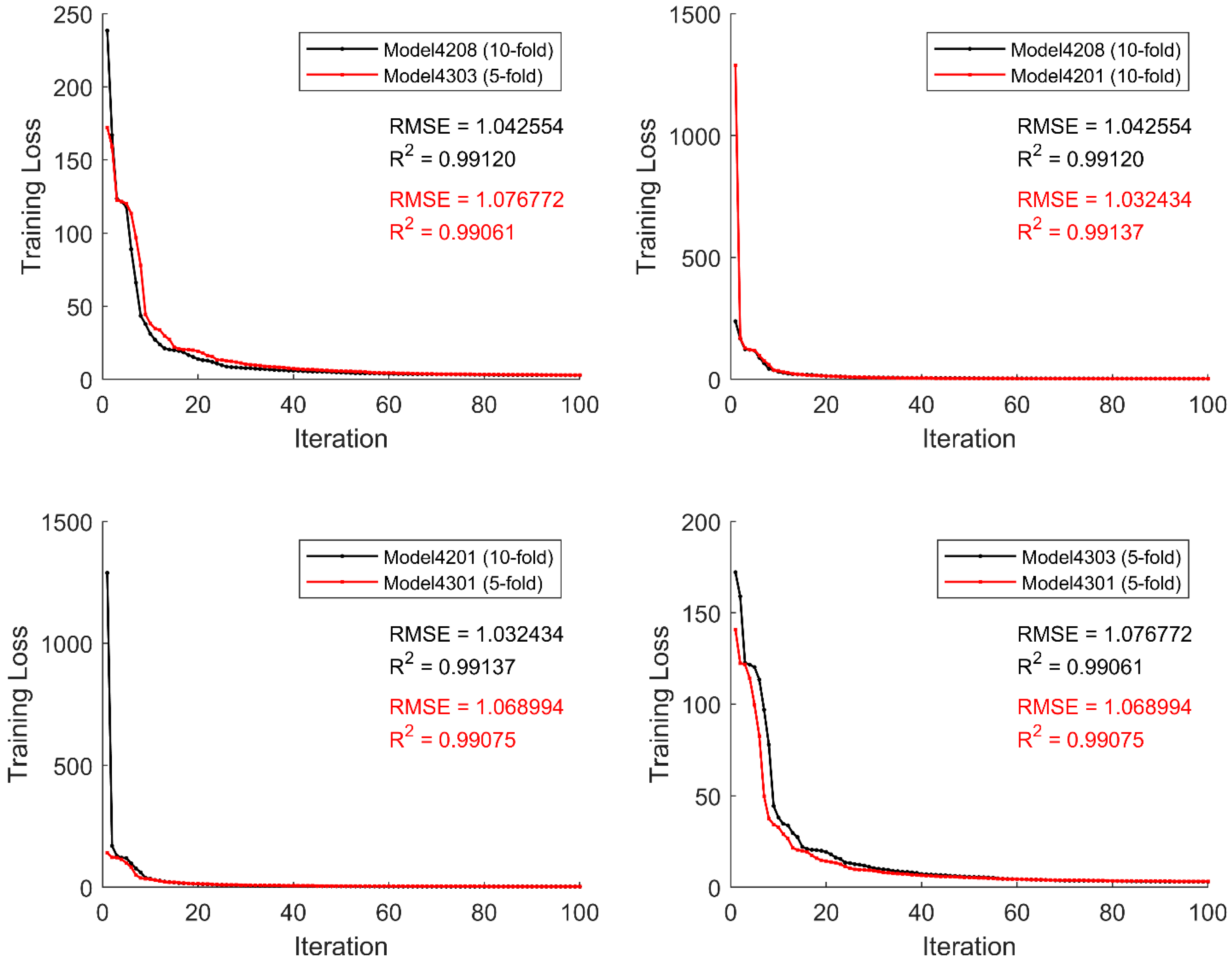
Figure 3.
Comparison of the training loss of the best five models from the five experimental runs.
Figure 3.
Comparison of the training loss of the best five models from the five experimental runs.
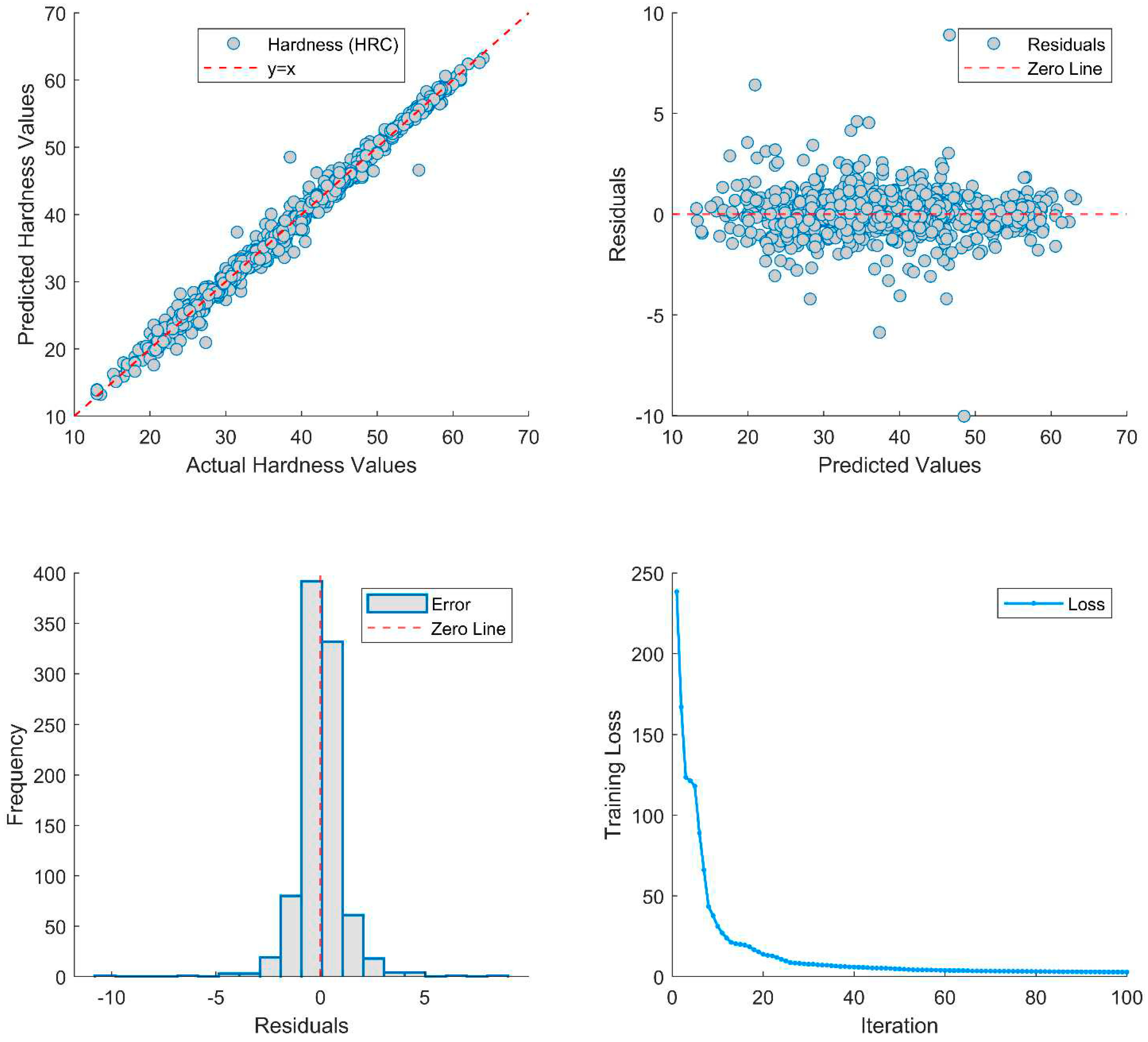
Figure 4.
Performance evaluation of Model II (model4301) on an unseen new test data set.
Figure 4.
Performance evaluation of Model II (model4301) on an unseen new test data set.
3.2. Experiment 1 and Experiment 2 Comparative Analysis
In Experiment 1, a 10-fold cross-validation approach was used to evaluate the performance of the model under different hyperparameter configurations. The parameters considered include the number of layers (NumLayers) from 1 to 2, activation functions (Activations) including ’relu’, ’tanh’, ’sigmoid’ and ’none’, standardization (Standardize) options of ’true’ or ’false’, regularization parameter (lambda) with values between 1.9172e-09 and 0.1, and the size of Layer 1 and Layer 2 ranging from 1 to 300. In Experiment 2, a 5-fold cross-validation was performed to evaluate the robustness of the model under the same hyperparameter variations. These experiments aimed to systematically investigate the effects of different configurations on the predictive performance of the model and to gain insights into the optimal hyperparameter settings for each regression task.
The process of identifying the optimal model for predicting hardness in the regression task involved three important steps. First, the fifteen best-performing models from each experiment were selected, highlighting their performance in the test datasets. Then, the selection was refined to the five best models. The results are shown in
Table 4 and
Table 5. In the final stage, a comparative analysis was performed between the best model from each experiment and the best models from the training datasets. Ultimately, the most effective test model was identified for subsequent prediction and deployment.
These results provide a comprehensive insight into the performance of the models under different cross-validation schemes and help to select the most effective models for predicting hardness in the regression task.
Based on the metrics provided on
Table 6, and
Figure 5 and
Figure 6, Model 4208 appears to outperform the other models, except for the mean absolute error (MAE). It achieves a relatively low MSE of 1.1643, indicating its ability to minimize the squared differences between predicted and actual values. The Root Mean Squared Error (RMSE) is also comparatively low at 1.0790, indicating accurate predictions with less variability. Although the MAE is slightly higher compared to some other models, it is still reasonable at 0.6938, indicating a relatively small average absolute error.
In addition, the Model 4208 has a high correlation coefficient (R) of 0.9950, indicating a strong linear relationship between the predicted and actual values. The coefficient of determination (R2) is 0.98996, which means that the model captures a substantial portion of the variance in the data. The standard deviation (STD) is 1.07898, which indicates a relatively low dispersion of the residuals.
The table displays the performance metrics of different models in predicting hardness. Each model is assessed based on various metrics, including Mean Squared Error (MSE), Root Mean Squared Error (RMSE), Mean Absolute Error (MAE), Correlation Coefficient (R), Coefficient of Determination (R2), Standard Deviation (STD), and Maximum Absolute Error (MaxAE).
To summarize, the Model 4208 is a promising candidate for hardness prediction. It shows a balanced performance on various metrics, with a particularly notable strength in minimizing the squared error and a high correlation with the actual data.
3.3. Illustrative Example of Model 4208 to Determine Hardenability Curves
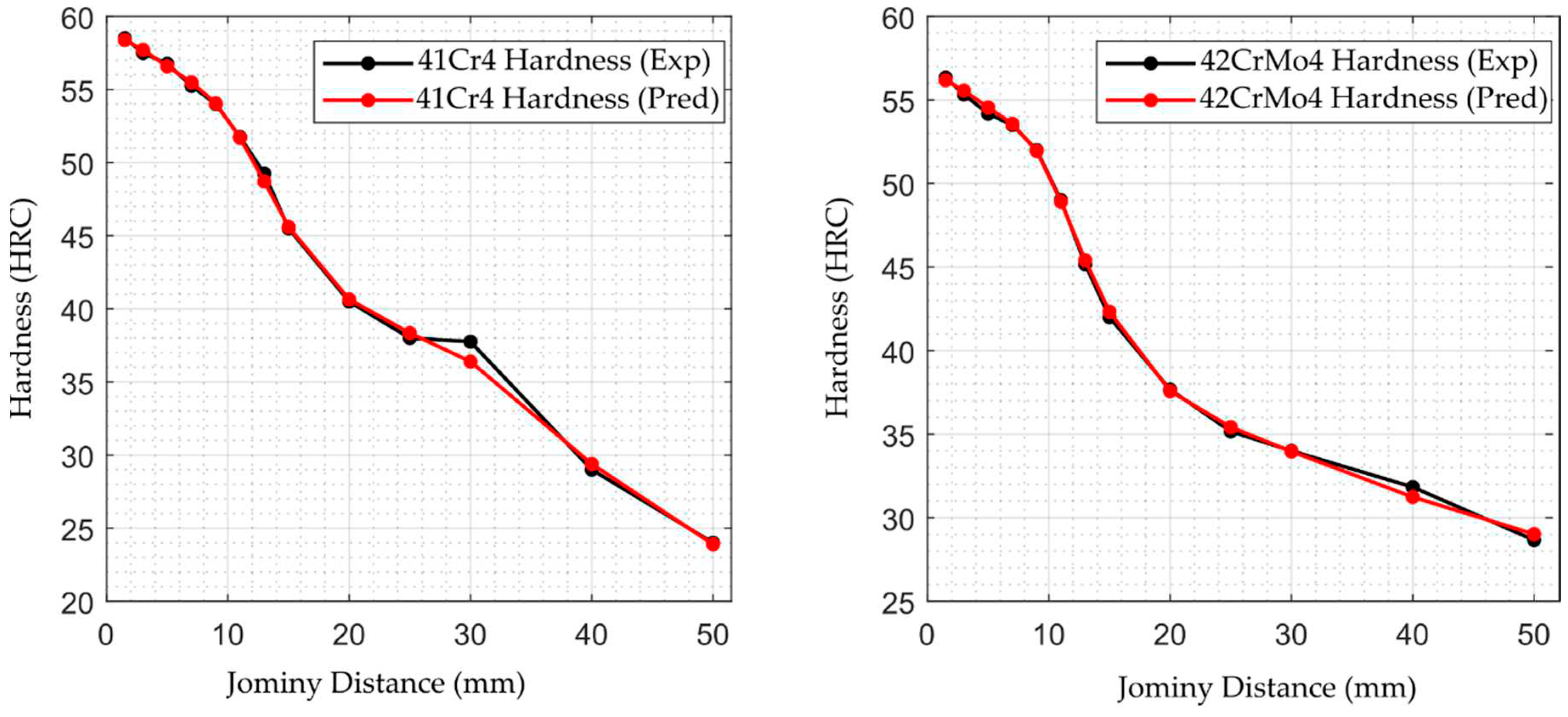
To evaluate the performance of the model, the hardenability curves of the 41Cr4 and 42CrMo4 steel grades are compared by examining the experimental and predicted results.
In this particular example, the performance of the model is evaluated by comparing the predicted hardness values with the observed (experimental) values for the 41Cr4 and 42CrMo4 steel grades. As evident from
Table 7 and
Figure 7, the results show close agreement between the experimental and predicted values. The close agreement between the experimental and predicted hardness values indicates a high degree of accuracy and reliability in the model’s ability to predict the hardenability of the steels. This robust predictive capability indicates the model’s potential for optimizing heat treatment processes, assisting in material selection, and improving overall efficiency in the design and manufacture of steel components.
3.4. Illustrative Example of Model 4208 to Determine Restricted Hardenability band of 42CrMo4 Steel Grade
In this section, the use case of the model in determining the hardenability band is discussed. Determining the H-band offers numerous advantages, including optimized material selection, enhanced component performance, cost-effective manufacturing, prevention of defects and failures, improved consistency and quality control, tailored material properties, and customization to specific customer requirements. Moreover, it aids in restricting the chemical composition ranges for applications and ensures the desired performance characteristics.
Due to variations in chemical composition among different heats of the same steel grade, hardenability bands are defined using the Jominy end-quench test. The upper curve indicates maximum hardness values corresponding to the upper composition limits, while the lower curve represents minimum hardness values for the lower composition limits. Hardenability bands are valuable for both suppliers and customers with most steels now purchased based on these bands. Suppliers ensure that a significant percentage, typically 93 or 95%, of mill heats meeting chemical specifications fall within the specified hardenability band [
43].
The model can be used either manually or can be combined with Bayesian Optimization or Genetic Algorithm [
14] to determine the limiting chemical compositions values within the required hardness stated by the customer. The integration of artificial neural networks with various modeling techniques such as mathematical modeling, computational intelligence, and artificial intelligence is a common practice. The amalgamation of different methods within a single model enables the exploration of a larger problem space and leads to a synergistic effect that utilizes the strengths of the individual methods [
23,
44].
Table 8 shows the chemical compositions determined comparing the 42CrMo4 steel grade hardness with DIN EN 10083-3 technical standard.
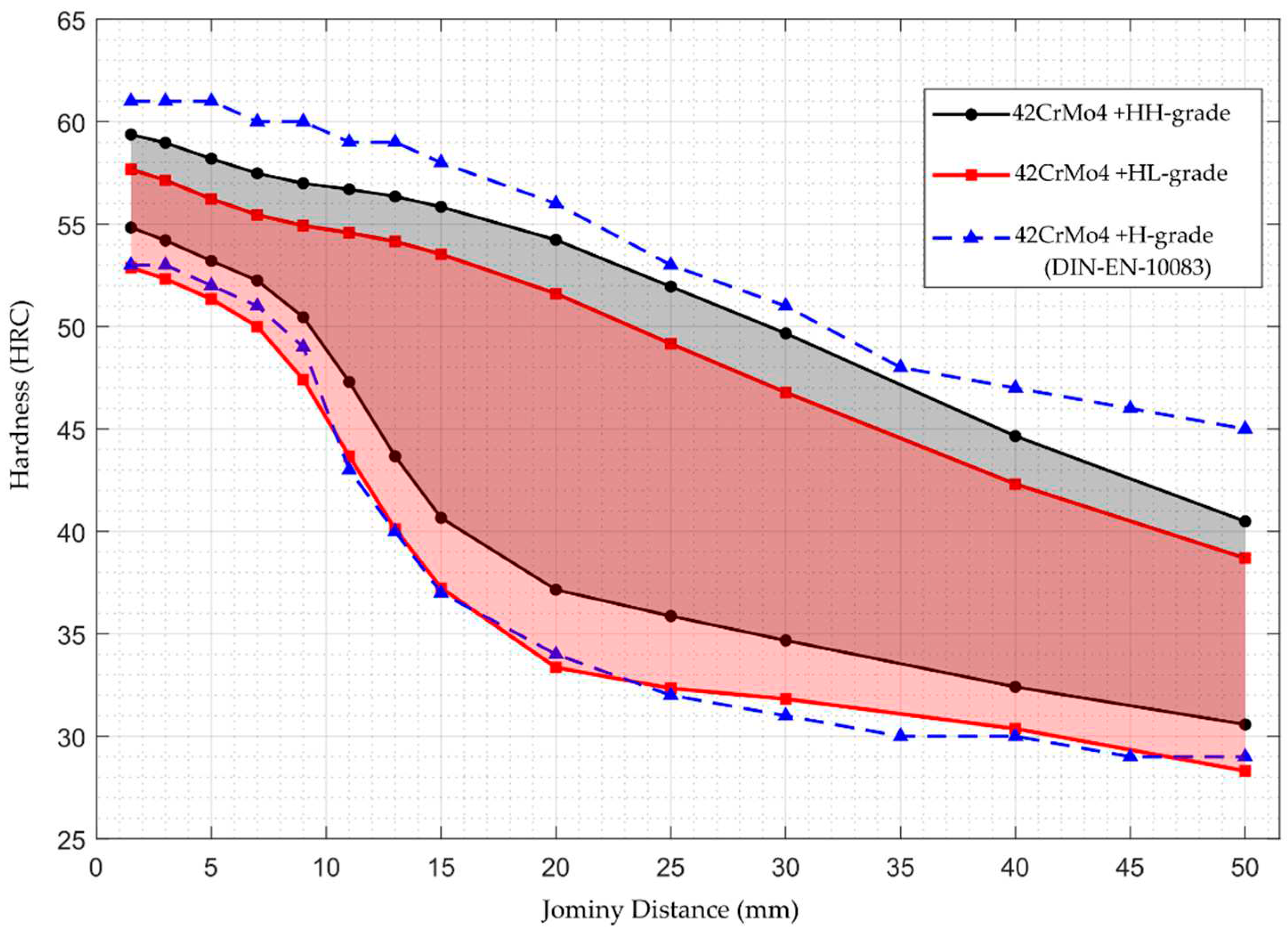
Table 9 shows the predicted maximum (Max) and minimum (Min) hardness values for the restricted hardenability towards the top of the scale (+HH) and restricted hardenability towards the bottom of the scale (+HL) bands of 42CrMo4 steel grade. The predicted values were determined using the developed model. In addition, the DIN EN 10083-3 provides reference values for the 42CrMo4 (+H) maximum (Max) and minimum (Min) hardness for comparison. This is visually depicted in
Figure 8 for enhanced clarity.
Comparing the predicted values with the standard reference values shows that the predictions of the model are generally within the specified hardness ranges, both for the Hardenability and Hardenability-Limited bands. The close agreement between the predicted values and standard values indicates that the model performs well in estimating the hardenability properties of the 42CrMo4 steel grade. This information is critical to ensure that the steel meets the specified hardness requirements for various applications and contributes to effective material selection and component design.
4. Discussion
The results obtained from the neural networks regression (fitrnet) models, particularly Model 4208 (8-85-141-1), demonstrate their remarkable effectiveness in predicting the hardness of steels. The rigorous hyperparameter tuning, facilitated by Bayesian optimization, contributes significantly to the performance of the models. The 5-fold and 10-fold cross-validation schemes ensure the reliability and generalizability of the models and provide robust insights into their predictive capabilities. When comparing various evaluation metrics such as mean square error (MSE), root mean square error (RMSE), mean absolute error (MAE), and coefficient of determination (R²), the 4208 model comes out on top. With an impressive RMSE of 1.0790 and an R² of 0.9900, the model demonstrates excellent accuracy and reliability across the assessment measures.
The illustrative example in the research paper shows the practical application of Model 4208 in determining the hardenability band for a particular steel grade. This application highlights the effectiveness of the model in predicting and optimizing heat treatment results and underscores its practical utility in materials engineering.
In summary, the experiments highlight the predictive capabilities of fitrnet models in determining the hardenability of steel, with Model 4208 demonstrating exceptional accuracy and robustness. The inclusion of Bayesian optimization improves the efficiency of hyperparameter tuning and highlights its importance in improving model performance.
5. Conclusions
The experiments conducted shed light on the effectiveness of the regression neural network (fitrnet) models in predicting steel hardness. The models, which were rigorously tuned using Bayesian optimization, have impressive predictive capabilities for steel hardness. Among the models, Model 4208 (8-85-141-1) stands out, demonstrating excellent accuracy and robustness across a range of assessment measures. The comprehensive cross-validation schemes (5-fold and 10-fold) ensure the reliability of the models and their generalization to unseen data. The inclusion of Bayesian optimization not only improves the efficiency of hyperparameter tuning but also highlights its importance in refining model performance. The performance of the model is also demonstrated through examples which show its effectiveness in tackling practical problems. This research provides valuable insights into the field of modeling material science and engineering properties. It highlights the potential of Regression Neural Networks in improving hardenability prediction and lays the foundation for future advances.
Author Contributions
Conceptualization, W.F.G. and W.S.; methodology, W.F.G; software, W.F.G.; validation, W.S. and G.F.B; formal analysis, W.F.G; investigation, W.S.; resources, W.S.; data curation, W.F.G. and W.S.; writing—original draft preparation, W.F.G.; writing—review and editing, G.F.B.; visualization, W.F.G.; supervision, W.S. All authors have read and agreed to the published version of the manuscript.
Funding
This research received no external funding.
Institutional Review Board Statement
Not applicable.
Informed Consent Statement
Not applicable.
Data Availability Statement
The dataset used to support the findings of this study is available from the corresponding author upon request.
Conflicts of Interest
The authors declare no conflicts of interest.
References
- Sitek, W.; Trzaska, J. Practical Aspects of the Design and Use of the Artificial Neural Networks in Materials Engineering. Metals 2021, 11. [Google Scholar] [CrossRef]
- Sitek, W.; Trzaska, J.; Gemechu, W.F. Modelling and Analysis of the Synergistic Alloying Elements Effect on Hardenability of Steel. Arch. Foundry Eng. [CrossRef]
- Rajan, K. Materials informatics. Mater. Today 2005, 8, 38–45. [Google Scholar] [CrossRef]
- Sha, W.X.; Guo, Y.Q.; Yuan, Q.; Tang, S.; Zhang, X.F.; Lu, S.F.; Guo, X.; Cao, Y.C.; Cheng, S.J. Artificial Intelligence to Power the Future of Materials Science and Engineering. Adv. Intell. Syst. 2020, 2. [Google Scholar] [CrossRef]
- Smoljan, B. Computer simulation of mechanical properties, stresses and strains of quenched steel specimen. J. Achiev. Mater. Manuf. Eng. 2006, 19. [Google Scholar]
- Homberg, D. A numerical simulation of the Jominy end-quench test. Acta Mater. 1996, 44, 4375–4385. [Google Scholar] [CrossRef]
- Li, M.V.; Niebuhr, D.V.; Meekisho, L.L.; Atteridge, D.G. A computational model for the prediction of steel hardenability. Metall. Mater. Trans. B-Process Metall. Mater. Process. Sci. 1998, 29, 661–672. [Google Scholar] [CrossRef]
- Vermeulen, W.G.; vanderWolk, P.J.; deWeijer, A.P.; vanderZwaag, S. Prediction of Jominy hardness profiles of steels using artificial neural networks. J. Mater. Eng. Perform. 1996, 5, 57–63. [Google Scholar] [CrossRef]
- Dobrzanski, L.A.; Sitek, W. Comparison of hardenability calculation methods of the heat-treatable constructional steels. J. Mater. Process. Technol. 1997, 64, 117–126. [Google Scholar] [CrossRef]
- Geng, X.X.; Wang, S.Z.; Ullah, A.; Wu, G.L.; Wang, H. Prediction of Hardenability Curves for Non-Boron Steels via a Combined Machine Learning Model. Materials 2022, 15. [Google Scholar] [CrossRef]
- Kovacic, M. Genetic Programming and Jominy Test Modeling. Mater. Manuf. Process. 2009, 24, 806–808. [Google Scholar] [CrossRef]
- Sponzilli, J.T.; Walter, G.H.; Doane, D.V. Development of Restricted Hardenability Band Steels. SAE Trans. 1987, 96, 1183–1190. [Google Scholar]
- Canale, L.C.F.; Albano, L.; Totten, G.E.; Meekisho, L. 12.03 - Hardenability of Steel. In Comprehensive Materials Processing; Hashmi, S., Batalha, G.F., Van Tyne, C.J., Yilbas, B., Eds.; Elsevier, 2014; pp. 39–97. [Google Scholar]
- Sitek, W.; Dobrzanski, L.A. Application of genetic methods in materials’ design. J. Mater. Process. Technol. 2005, 164, 1607–1611. [Google Scholar] [CrossRef]
- Mukherjee, M.; Singh, S.B. Artificial Neural Network: Some Applications in Physical Metallurgy of Steels. Mater. Manuf. Process. 2009, 24, 198–208. [Google Scholar] [CrossRef]
- Liu, Y.; Zhao, T.L.; Ju, W.W.; Shi, S.Q. Materials discovery and design using machine learning. J. Mater. 2017, 3, 159–177. [Google Scholar] [CrossRef]
- Mueller, T.; Kusne, A.G.; Ramprasad, R. MACHINE LEARNING IN MATERIALS SCIENCE: RECENT PROGRESS AND EMERGING APPLICATIONS. Rev. Comput. Chem. Vol 29 2016, 29, 186–273. [Google Scholar]
- Wei, J.; Chu, X.; Sun, X.Y.; Xu, K.; Deng, H.X.; Chen, J.G.; Wei, Z.M.; Lei, M. Machine learning in materials science. Infomat 2019, 1, 338–358. [Google Scholar] [CrossRef]
- Chan, C.H.; Sun, M.Z.; Huang, B.L. Application of machine learning for advanced material prediction and design. Ecomat 2022, 4. [Google Scholar] [CrossRef]
- Sha, W.; Edwards, K.L. The use of artificial neural networks in materials science based research. Mater. Des. 2007, 28, 1747–1752. [Google Scholar] [CrossRef]
- Bhadeshia, H. Neural networks in materials science. Isij Int. 1999, 39, 966–979. [Google Scholar] [CrossRef]
- Bhadeshia, H.; Dimitriu, R.C.; Forsik, S.; Pak, J.H.; Ryu, J.H. Performance of neural networks in materials science. Mater. Sci. Technol. 2009, 25, 504–510. [Google Scholar] [CrossRef]
- Trzaska, J.; Sitek, W. A Hybrid Method for Calculating the Chemical Composition of Steel with the Required Hardness after Cooling from the Austenitizing Temperature. Materials 2024, 17. [Google Scholar] [CrossRef] [PubMed]
- Bishop, C.M.; Bishop, H. The Deep Learning Revolution. In Deep Learning: Foundations and Concepts; Springer International Publishing, 2024; pp. 1–22. [Google Scholar]
- Hanza, S.S.; Marohnic, T.; Iljkic, D.; Basan, R. Artificial Neural Networks-Based Prediction of Hardness of Low-Alloy Steels Using Specific Jominy Distance. Metals 2021, 11. [Google Scholar] [CrossRef]
- Reddy, N.S.; Krishnaiah, J.; Hong, S.G.; Lee, J.S. Modeling medium carbon steels by using artificial neural networks. Mater. Sci. Eng. A-Struct. Mater. Prop. Microstruct. Process. 2009, 508, 93–105. [Google Scholar] [CrossRef]
- Dobrzanski, L.A.; Sitek, W. Application of a neural network in modelling of hardenability of constructional steels. J. Mater. Process. Technol. 1998, 78, 59–66. [Google Scholar] [CrossRef]
- Santhosh, A.J.; Tura, A.D.; Jiregna, I.T.; Gemechu, W.F.; Ashok, N.; Ponnusamy, M. Optimization of CNC turning parameters using face centred CCD approach in RSM and ANN-genetic algorithm for AISI 4340 alloy steel. Results Eng. 2021, 11. [Google Scholar] [CrossRef]
- de Zarza, I.; de Curtò, J.; Calafate, C.T. Optimizing Neural Networks for Imbalanced Data. Electronics 2023, 12. [Google Scholar] [CrossRef]
- Fontanari, T.; Fróes, T.C.; Recamonde-Mendoza, M. Cross-validation Strategies for Balanced and Imbalanced Datasets. Intell. Syst. Pt I 2022, 13653, 626–640. [Google Scholar] [CrossRef]
- James, G.; Witten, D.; Hastie, T.; Tibshirani, R.; Taylor, J. Resampling Methods. In An Introduction to Statistical Learning: with Applications in Python; Springer Texts in Statistics (STS); Springer International Publishing, 2023; pp. 201–228. [Google Scholar]
- Breiman, L.; Spector, P. SUBMODEL SELECTION AND EVALUATION IN REGRESSION - THE X-RANDOM CASE. Int. Stat. Rev. 1992, 60, 291–319. [Google Scholar] [CrossRef]
- Bischl, B.; Binder, M.; Lang, M.; Pielok, T.; Richter, J.; Coors, S.; Thomas, J.; Ullmann, T.; Becker, M.; Boulesteix, A.L.; et al. Hyperparameter optimization: Foundations, algorithms, best practices, and open challenges. Wiley Interdiscip. Rev. -Data Min. Knowl. Discov. 2023, 13. [Google Scholar] [CrossRef]
- Snoek, J.; Larochelle, H.; Adams, R.P. Practical Bayesian optimization of machine learning algorithms. 2012. [CrossRef]
- Bhandari, U.; Chen, Y.H.; Ding, H.; Zeng, C.Y.; Emanet, S.; Gradl, P.R.; Guo, S.M. Machine-Learning-Based Thermal Conductivity Prediction for Additively Manufactured Alloys. J. Manuf. Mater. Process. 2023, 7. [Google Scholar] [CrossRef]
- Snoek, J.; Larochelle, H.; Adams, R.P. Practical Bayesian optimization of machine learning algorithms. In Proceedings of the Advances in Neural Information Processing Systems 25 (NIPS 2012); 2012; pp. 2960–2968. [Google Scholar]
- Lee, S.Y.; Byeon, S.; Kim, H.S.; Jin, H.; Lee, S. Deep learning-based phase prediction of high-entropy alloys: Optimization, generation, and explanation. Mater. Des. 2021, 197. [Google Scholar] [CrossRef]
- Inc., T.M. Statistics and machine learning toolbox. 2023. 2023.
- Feurer, M.; Hutter, F. Hyperparameter Optimization. In Automated Machine Learning: Methods, Systems, Challenges; Hutter, F., Kotthoff, L., Vanschoren, J., Eds.; The Springer Series on Challenges in Machine Learning; Springer International Publishing, 2019; pp. 3–33. [Google Scholar]
- Jones, D.R.; Schonlau, M.; Welch, W.J. Efficient global optimization of expensive black-box functions. J. Glob. Optim. 1998, 13, 455–492. [Google Scholar] [CrossRef]
- Kim, Y.; Chung, M. An Approach to Hyperparameter Optimization for the Objective Function in Machine Learning. Electronics 2019, 8. [Google Scholar] [CrossRef]
- Massey, F.J. THE KOLMOGOROV-SMIRNOV TEST FOR GOODNESS OF FIT. J. Am. Stat. Assoc. 1951, 46, 68–78. [Google Scholar] [CrossRef]
- Liscic, B. Hardenability. In Steel Heat Treatment Handbook - 2 Volume Set, 2nd ed.; Totten, G.E., Ed.; CRC Press, 2007; pp. 213–276. [Google Scholar]
- Datta, S.; Chattopadhyay, P.P. Soft computing techniques in advancement of structural metals. Int. Mater. Rev. 2013, 58, 475–504. [Google Scholar] [CrossRef]
|
Disclaimer/Publisher’s Note: The statements, opinions and data contained in all publications are solely those of the individual author(s) and contributor(s) and not of MDPI and/or the editor(s). MDPI and/or the editor(s) disclaim responsibility for any injury to people or property resulting from any ideas, methods, instructions or products referred to in the content. |
© 2024 by the authors. Licensee MDPI, Basel, Switzerland. This article is an open access article distributed under the terms and conditions of the Creative Commons Attribution (CC BY) license (http://creativecommons.org/licenses/by/4.0/).
