Explicit P1 Finite Element Solution of the Maxwell-Wave Equation Coupling Problem with Absorbing b. c.

1. Introduction

The aim of this article is to show that an explicit $P_1$ lumped-mass finite-element scheme can be a reliable method to solve the Maxwell’s equations of electromagnetism in the time domain and in a bounded domain in ${\Re }^N$, $N=2,3$. This fact is illustrated here assuming a constant magnetic permeability. It is well known that in this case these equations can be expressed as a second order system in terms of the sole electric field. Moreover, the study is conducted in the particular case where the dielectric permittivity is constant in a region of the computational domain contiguous to its boundary. As a consequence, the wave equation holds therein and for this reason we address the case of a coupling problem for the Maxwell’s equations in the inner domain and the wave equation in the outer domain. However, if it happens that the Maxwell system also holds in the latter, then our study will directly apply to the Maxwell’s equations in the whole domain. Moreover, although it extends to other boundary conditions with minor modifications, as a model we consider in this work first-order absorbing boundaryboundary conditions.

Standard conforming linear finite elements are a priori an attractive tool to solve Maxwell’s equations, as an inexpensive method, especially in three-dimension space. However, this is not always a good choice for such a purpose. A primary explanation for this assertion is the fact that in geneoral the electric field cannot be searched for in the Sobolev space ${\left\{H^1\right\}}^N$, but rather in a subspace of $\mathbf{H}\left(curl\right)\cap \mathbf{H}\left(div\right)$ consisting of vector fields satisfying certain boundary conditions. As a consequence, if the spacial domain in which the equations are defined has re-entrant corners, the subspace of ${\left\{H^1\right\}}^N\cap (\mathbf{H}\left(curl\right)\cap \mathbf{H}\left(div\right))$, incorporating for instance zero tangential boundary conditions, is a proper subspace of the corresponding subspace of $\mathbf{H}\left(curl\right)\cap \mathbf{H}\left(div\right)$ owing to the so-called corner paradox (see e.g. [19,20]). This was one of the main motivations of different authors who looked into the design of finite element methods to cope with the issue. A celebrated contribution in this direction is due to Nédélec [29], namely, a family of $\mathbf{H}\left(curl\right)$-conforming methods to solve these equations, commonly known as edge elements. The crucial point in the discussion on discretization methods to tackle the problem, is how to get rid of spurious solutions and other instabilities usually caused by nodal elements, such as the $P_1$ FEM. A detailed study of these questions, together with methods especially designed to solve Maxwell’s equations is given for instance in [10,28]. A more recent approach to handle these equations using a Hermite variant of the lowest order Raviart-Thomas interpolation [30] was reported in [32].

In this work we rule out the aforementioned shortcoming, by taking advantage of the fact that the solution of the wave equation lies in ${\left\{H^1\right\}}^N$ irrespective of boundary conditions. Hence in our case we can show that the $P_1$ finite element method is indeed an accurate numerical solution tool, provided the coupled equations are written in a suitable VF (variational form). Actually, the VF employed in this work is similar but not equal to the AVF-Augmented Variational Formulation thoroughly studied by Ciarlet Jr. (cf. [16]) in the static and time-harmonic cases and in Jamelot [27] and Ciarlet Jr.-Jamelot [17]) in the time-dependent case. However, non negligible additional complexities must be dealt with, stemming from the fact that the dielectric permittivity varies in space. This is one of the main reasons that compelled the authors to carry out here a rigorous analysis of the $P_1$ lumped-mass approximation of Maxwell’s equations. As a matter of fact, to the best of their knowledge, such results were lacking. Indeed, the case of a variable dielectric permittivity had been addressed in [18,23], but not for nodal finite elements, while in [2,15,17] nodal finite elements are dealt with, though for constant coefficients and formulations different from ours.

Conforming nodal finite elements were considered to handle the time-dependent case in the early nineties (cf. [2]) for convex domains. Later on specialists studied formulations of the static or the time-harmonic Maxwell’s equations suitable for a numerical solution with nodal elements, even for non convex domains. In this respect we refer to [3,17,21,27]. Such studies revealed the adequacy of nodal elements, at least in some relevant practical situations. Underlying this work lies precisely one such a case, characterized by the fact that the dielectric permittivity is constant in a neighborhood of the boundary of the domain of interest. On the other hand we emphasize again that there are not many studies of nodal elements as applied to the time-dependent Maxwell’s equations with variable coefficients. Hence this paper also gives a contribution in this direction. In short, by applying a lumped-mass explicit $P_1$ finite-elements scheme to the Maxwell’s equations in terms of the electric field recast in a suitable VF, we establish that, at least in the above case, reliable numerical solutions are generated, as long as a classical stability condition is fulfilled.

Before pursuing, it should be pointed out that we had described and assessed our method in [7,8], without giving mathematical proofs of reliability. Here we present the main lines of its formal numerical analysis, though not for the same boundary conditions. For this reason the numerical examples shown in both articles are different from those presented in this work. We also observe that, akin to [8], we study here a Maxwell-wave equation coupling problem posed in two contiguous disjoint sub-domains, which happens to simplify into Maxwell’s equations in the union of both sub-domains under certain conditions. The mathematical grounds of our VF, in particular its equivalence with the strong form of the Maxwell’s equations, follows the main lines of [8].

As a matter of fact, this work somehow validates a numerical solution procedure described in [4] applied to a kind of CIP - Coefficient Inverse Problem - for the time-dependent Maxwell’s equations in the particular configuration underlined above. Let us briefly recall it below. For more details we refer to [9] and references therein.

Assume that in a vast nonconducting homogeneous medium with a given dielectric permittivity, an unknown object is searched for. The object’s material is also supposedly nonconducting, though with a different dielectric permittivity. Solenoidal electric waves of a regular pattern are emitted sufficiently far away from the search region during a certain time. In the absence of a hidden object such a pattern will be observed during all time in a certain location closer to the search zone. However, if there is indeed a hidden object, waves will be reflected and back-scattered onto the observation zone. Schematically such a process may be thought of as governed by the Maxwell system of equations of electromagnetism in an unbounded domain with a constant dielectric permittivity, except in a region surrounding the hidden object where the dielectric permittivity varies. The CIP consists of determining the spacial distribution of an unknown dielectric permittivity - i.e., a coefficient of Maxwell’s equations, - with the aim of locating the hidden object, on the basis of measurements of back-scattered waves at a small observation zone. In principle, the far electric field will still be as regular as the emitted one. However, we may conveniently solve the problem by taking a bounded computational domain consisting of two sub-domains, namely, an inner domain where the hidden object lies, and a surrounding outer domain on whose outer boundary - that is, the boundary of the computational domain, - absorbing boundary conditions are prescribed (see e.g. [22,24]). It is noticeable that, since the dielectric permittivity is constant in the outer domain, N wave equations hold therein. Moreover, since the far field is solenoidal, in practical terms it can be thought of as being also solenoidal on the boundary of the computational domain, as long as it is large enough. However, strictly speaking, such a condition cannot be prescribed, and hence it is mathematically inconsistent to consider that the full Maxwell system of equations hold in the outer domain, as it does in the inner domain. That is why we address in this article a Maxwell-wave coupling problem posed simultaneouly in the inner and the outer sub-domains, bearing in mind that, at least for the CIP in view, Maxwell’s equations are expected to hold in the union of both.

An outline of this paper is as follows: In Section 2 we describe the model problem being solved and study its equivalent VF employed in the sequel. In Section 3 we set up the discretizations of the model problem in both space and time. Section 4 is devoted to the formal reliability analysis of the explicit scheme considered in the previous section. A priori error estimates are given therein under the realistic assumption that the time step varies linearly with the mesh size as the mesh is refined. In Section 5 we present a numerical validation of our scheme. Finally we conclude in Section 6 with a few comments on the whole work.

2. The model problem

The Maxwell-wave equation coupling problem for a field $\mathbf{e}$ in a bounded Lipschitz domain $\Omega$ of ${\Re }^N,N=2,3$ with boundary $\Gamma$, that we consider in this work is posed in the following setting.

• First, we consider that $\Omega ={\overline{\Omega }}_{in}\cup {\Omega }_{out}$, where ${\Omega }_{in}$ is an interior open set whose boundary ${\Gamma }_{in}$ does not intersect $\Gamma$ and ${\Omega }_{out}$ is the complementary set of ${\overline{\Omega }}_{in}$ with respect to $\Omega$ (the boundary of ${\Gamma }_{out}$ is $\Gamma \cup {\Gamma }_{in}$). The dielectric permittivity denoted by $\epsilon$ is assumed to belong to $C^2\left(\overline{\Omega }\right)$ and to fulfill the conditions:

$$\epsilon \equiv 1 \mathrm{in} {\Omega }_{\mathit{out}} \mathrm{and} \epsilon \ge 1 \mathrm{otherwise}.$$

(2.1)

Let $\mathbf{n}$ be the unit outer normal vector on $\Gamma$. We denote by ${\partial }_n(·)$ the outer normal derivative of a field on $\Gamma$. Taking into account conditions (2.1), we may prescribe wave-equation first order absorbing boundary conditions ${\partial }_n\mathbf{e}=-{\partial }_t\mathbf{e}$ on $\Gamma \times (0,T)$ [22,24], as seen hereafter.

Now, we are given ${\mathbf{e}}_0\in {\left\{H^1(\Omega )\right\}}^N$ and ${\mathbf{e}}_1\in \mathbf{H}(div,\Omega )$ satisfying $\nabla ·\left(\epsilon {\mathbf{e}}_0\right)=\nabla ·\left(\epsilon {\mathbf{e}}_1\right)\equiv 0$, together with $\mathbf{f}\in L^2[(0,T);\mathbf{H}(div,\Omega )]$ satisfying $\nabla ·\mathbf{f}\equiv 0$. Then, setting $\mathbf{V}:={\left\{H^1(\Omega )\right\}}^N$, the problem to solve is:

$$\left\{\begin{array}{cc}\mathrm{Find} \mathbf{e}\in \mathcal{V}:=H^2[(0,T);{\left\{L^2(\Omega )\right\}}^N]\cap L^2[(0,T);\mathbf{V}]\hfill & \\ \mathrm{such} \mathrm{that}\hfill & \\ \left.\begin{array}{c}\epsilon {\partial }_{tt}\mathbf{e}+\nabla \times \nabla \times \mathbf{e}=\mathbf{f},\hfill \\ \nabla ·\left\{\epsilon \mathbf{e}\right\}=0.\hfill \end{array}\right\}\hfill & \mathrm{in} {\Omega }_{in}\times (0,T),\hfill \\ {\partial }_{tt}\mathbf{e}-\Delta \mathbf{e}=\mathbf{f}\hfill & \mathrm{in} {\Omega }_{out}\times (0,T),\hfill \\ \mathrm{with} \mathrm{the} \mathrm{initial} \mathrm{conditions}\hfill & \\ \mathbf{e}(·,0)={\mathbf{e}}_0(·), \mathrm{and} {\partial }_t\mathbf{e}(·,0)={\mathbf{e}}_1(·)\hfill & \mathrm{in} \Omega \hfill \\ \mathrm{and} \mathrm{the} \mathrm{boundary} \mathrm{conditions}\hfill & \\ {\partial }_n\mathbf{e}+{\partial }_t\mathbf{e}=\mathbf{0}\hfill & \mathrm{on} \Gamma \times (0,T).\hfill \end{array}\right.$$

(2.2)

(2.2) tells us that the wave equation holds in ${\Omega }_{out}\times (0,T)$. On the other hand, the equations in braces of (2.2) make up the Maxwell’s equations in ${\Omega }_{in}\times (0,T)$ for the sole electric field. It is noticeable that, since $\mathbf{f}$ is solenoidal by assumption, the second equation in ${\Omega }_{in}\times (0,T)$ is superfluous i.e. reduntant. Indeed, taking the divergence of both sides of the first equation in ${\Omega }_{in}\times (0,T)$ and denoting by u the function $\nabla ·\left(\epsilon \mathbf{e}\right)$, we have ${\partial }_{tt}u=0 \mathrm{in} {\Omega }_{in}\times (0,T)$. Taking into account that $u_{|t=0}={{\partial }_{t}u}_{|t=0}=0$ by our assumption on ${\mathbf{e}}_0$ and ${\mathbf{e}}_1$, it must hold $\nabla ·\left(\epsilon \mathbf{e}\right)=0$ in ${\Omega }_{in}\times (0,T)$. However, the same conclusion cannot be drawn for ${\Omega }_{out}\times (0,T)$. This is because in this sub-domain $u:=\nabla ·\mathbf{e}$ solves a wave equation $u_{tt}-\Delta u=0$ with zero initial conditions. Since zero boundary conditions do not necessarily hold for u, this is not sufficient to infer that $u\equiv 0$ in ${\Omega }_{out}\times (0,T)$. But, of course, nothing prevents the Maxwell’s equations from holding indeed in this domain too, as pointed out at the end of Section 1.

2.1. Notations and reminders

Before pursuing we introduce some notations and recall a couple of results to be used hereafter.

We denote the standard semi-norm of $C^n\left(\overline{\Omega }\right)$ by ${|·|}_{n,\infty }$ for $n>0$ and the standard norm of $C^0\left(\overline{\Omega }\right)$ by ${\parallel ·\parallel }_{0,\infty }$. A subset of $\overline{\Omega }$ will be denoted by an upper case Latin letter with or without a subscript. For any $D\subset \Omega$ we denote the standard inner product of ${\left\{L^2\left(D\right)\right\}}^N$ by ${(·,·)}_D$ and the corresponding norm by ${\Vert \{·\}\Vert }_D$; if $D=\Omega$ we drop the subscript D. $meas\left(D\right)$ represents the measure of D, which accounts for the length, the area or the volume of D, according to the case.

• Any scalar function defined in $\Omega$ will be denoted by a lower case Greek letter combined or not with other symbols different from upper case letters. For a given non negative function $\omega \in L^{\infty }(\Omega )$ we introduce the weighted $L^2(\Omega )$-semi-norm ${\parallel \{·\}\parallel }_{\omega }:=\sqrt{{\int }_{\Omega }\omega {|\{·\}|}^2}$, which is actually a norm if $\omega \ne 0$ everywhere in $\overline{\Omega }$. The notation ${(\mathcal{A},\mathcal{B})}_{\omega }$ expresses ${\int }_{\Omega }\omega \mathcal{A}·\mathcal{B}$, $\mathcal{A},\mathcal{B}$ being two square-integrable fields in $\Omega$. If $\omega$ is strictly positive this expression defines an inner product associated with the norm ${\parallel \{·\}\parallel }_{\omega }$.
• We denote by $<·,·{>}_{s,{\Gamma }_{in}}$ the duality product of $H^s\left({\Gamma }_{in}\right)-H^{-s}\left({\Gamma }_{in}\right)$ for $s\in {\Re }^{+}$.

In the sequel we shall repeatedly employ a well known operator identity applying to vector fields, namely,

$$-\Delta \equiv -\nabla \nabla ·+\nabla \times \nabla \times .$$

(2.3)

Let D be a bounded domain of ${\Re }^N$ with boundary $\partial D$. We recall that, according to the Trace Theorem (cf. [1]) and well known results, if a given function $\chi \in L^2\left(D\right)$ has a well defined trace on $\partial D$ in the space $H^{1/2}(\partial D)$ and $\Delta \chi \in H^{-1}\left(D\right)$, then necessarily $\chi \in H^1\left(D\right)$.

2.2. Well-posedness considerations

The well-posedness of (2.2) will be taken for granted. However, it can be established by means of an argument similar to the one exploited in [8]. Since it is rather laborious, for the sake of brevity we skip details of such an analysis. Nevertheless we next sketch its main lines, which rely on the well-posedness of the following problem.

• Let $\mathbf{R}:=\{(\mathbf{v},\mathbf{z})|\mathbf{v}\in {\left\{H^1\left({\Omega }_{out}\right)\right\}}^N,\mathbf{z}\in \mathbf{H}(curl;{\Omega }_{in})\cap \mathbf{H}(div;{\Omega }_{in}),{\int }_{{\Omega }_{out}}\mathbf{u}+{\int }_{{\Omega }_{in}}\mathbf{w}=\mathbf{0}\}$ and let ${\mathbf{R}}_{\epsilon }$ be the subspace of $\mathbf{R}$ of the pairs $(\mathbf{v};\mathbf{z})$ satisfying $\nabla ·\left(\epsilon \mathbf{z}\right)=0$ in ${\Omega }_{in}$. Noticing that the trace over ${\Gamma }_{in}$ of a field in $\mathbf{H}(curl;{\Omega }_{in})\cap \mathbf{H}(div;{\Omega }_{in})\}$ lies in ${\left\{H^{-1/2}\left({\Gamma }_{in}\right)\right\}}^N$ (cf. [25]), recalling the space $L_0^2(\Omega ):=\{v|v\in L^2(\Omega ),{\int }_{\Omega }v=0\}$, we set the problem

$$\left\{\begin{array}{c}\mathrm{Given} \mathrm{a} \mathrm{solenoidal} \mathbf{g}\in {\left\{L_0^2(\Omega )\right\}}^N \mathrm{find} ((\mathbf{u};\mathbf{w});\mathbf{p})\in {\mathbf{R}}_{\epsilon }\times {\left\{H^{1/2}\left({\Gamma }_{in}\right)\right\}}^N\hfill \\ \mathrm{such} \mathrm{that} \forall ((\mathbf{v};\mathbf{z});\mathbf{q})\in {\mathbf{R}}_{\epsilon }\times {\left\{H^{1/2}\left({\Gamma }_{in}\right)\right\}}^N\hfill \\ {(\nabla \mathbf{u},\nabla \mathbf{v})}_{{\Omega }_{out}}+{(\nabla \times \mathbf{w},\nabla \times \mathbf{z})}_{{\Omega }_{in}}+<\mathbf{p},\mathbf{v}-\mathbf{z}{>}_{1/2,{\Gamma }_{in}}={({\mathbf{g}}_{|{\Omega }_{out}},\mathbf{v})}_{{\Omega }_{out}}+{({\mathbf{g}}_{|{\Omega }_{in}},\mathbf{z})}_{{\Omega }_{in}},\hfill \\ <\mathbf{q},\mathbf{u}-\mathbf{w}{>}_{1/2,{\Gamma }_{in}}=0.\hfill \end{array}\right.$$

(2.4)

Using the theory of saddle-point linear problems (cf. [11]) we have checked that (2.4) has a unique solution and moreover, by the same theory, it is equivalent to the following system:

$$\left\{\begin{array}{c}\mathrm{Given} \mathrm{a} \mathrm{solenoidal} \mathbf{g}\in {\left\{{\mathbf{L}}_0^2(\Omega )\right\}}^N, \mathrm{find} ((\mathbf{u};\mathbf{w});r;\mathbf{p})\in \mathbf{R}\times L^2\left({\Omega }_{in}\right)\times {\left\{H^{1/2}\left({\Gamma }_{in}\right)\right\}}^N\hfill \\ \mathrm{such} \mathrm{that} \forall \left((\mathbf{v};\mathbf{z})\right);s;\mathbf{q})\in \mathbf{R}\times L^2\left({\Omega }_{in}\right)\times {\left\{H^{1/2}\left({\Gamma }_{in}\right)\right\}}^N\hfill \\ {(\nabla \mathbf{u},\nabla \mathbf{v})}_{{\Omega }_{out}}+{(\nabla \times \mathbf{w},\nabla \times \mathbf{z})}_{{\Omega }_{in}}+{(r,\nabla ·\left(\epsilon \mathbf{z}\right))}_{{\Omega }_{in}}+<\mathbf{p},\mathbf{v}-\mathbf{z}{>}_{1/2,{\Gamma }_{in}}\hfill \\ ={({\mathbf{g}}_{|{\Omega }_{out}},\mathbf{v})}_{{\Omega }_{out}}+{({\mathbf{g}}_{|{\Omega }_{in}},\mathbf{z})}_{{\Omega }_{in}},\hfill \\ {(\nabla ·\left(\epsilon \mathbf{w}\right),s)}_{{\Omega }_{in}}=0,\hfill \\ <\mathbf{q},\mathbf{u}-\mathbf{w}{>}_{1/2,{\Gamma }_{in}}=0..\hfill \end{array}\right.$$

(2.5)

It is clear that the solution of (2.5) solves the following problem:

$$\left\{\begin{array}{cc}\mathrm{Given} \mathbf{g}\in {\left\{{\mathbf{L}}_0^2(\Omega )\right\}}^N \mathrm{fulfilling} \nabla ·\mathbf{g}=0 \mathrm{in} \Omega ,\hfill & \mathrm{find} (\mathbf{u};\mathbf{w})\in \mathbf{R} \mathrm{such} \mathrm{that}\hfill \\ -\Delta \mathbf{u}={\mathbf{g}}_{|{\Omega }_{out}}\hfill & \mathrm{in} {\Omega }_{out}\hfill \\ \left.\begin{array}{c}\nabla \times \nabla \times \mathbf{w}={\mathbf{g}}_{|{\Omega }_{in}},\hfill \\ \nabla ·\left(\epsilon \mathbf{w}\right)=0.\hfill \end{array}\right\}\hfill & \mathrm{in} {\Omega }_{in},\hfill \\ \mathbf{u}=\mathbf{w}\hfill & \mathrm{on} {\Gamma }_{in},\hfill \\ {\partial }_n\mathbf{u}=\mathbf{0}\hfill & \mathrm{on} \Gamma ,\hfill \\ {\int }_{{\Omega }_{out}}\mathbf{u}+{\int }_{{\Omega }_{in}}\mathbf{w}=\mathbf{0}.\hfill \end{array}\right.$$

(2.6)

Thus, from classical results (cf. [13]), any linear second order hyperbolic counterpart of (2.6) assorted with proper initial conditions also has a unique solution. Let us consider a field $\mathbf{e}$ defined in $\Omega$ such that ${\mathbf{e}}_{|{\Omega }_{out}}=\mathbf{u}$ and ${\mathbf{e}}_{|{\Omega }_{in}}=\mathbf{w}$. Since $\nabla ·\mathbf{w}=-\nabla log\left(\epsilon \right)·\mathbf{w}\in L^2\left({\Omega }_{in}\right)$ from the assumed regularity of $\epsilon$, we have $\nabla \nabla ·\mathbf{w}\in {\left\{H^{-1}\left({\Omega }_{in}\right)\right\}}^N$. This implies that $\Delta \mathbf{w}\in {\left\{H^{-1}\left({\Omega }_{in}\right)\right\}}^N$ by the identity (2.3), since $\nabla \times \nabla \times \mathbf{w}\in \{L^2{\left({\Omega }_{in}\right\}}^N$. Therefore $\mathbf{w}\in {\left\{H^1\left({\Omega }_{in}\right)\right\}}^N$ owing to the coincidence of $\mathbf{u}$ and $\mathbf{w}$ on ${\Gamma }_{in}$. Hence $\mathbf{e}$ lies in ${\left\{H^1(\Omega )\right\}}^N$ and moreover it solves a well-posed elliptic problem in $\Omega$. Thus the well-posedness of (2.2) follows from the fact that it is a second order hyperbolic counterpart of (2.6).

Remark 2.1.

As already pointed out in Section 1, the study that follows also applies to several types of boundary conditions, for which such an $H^1$-regularity is known to hold. As pointeed out in Section 1, the choice of absorbing boundary conditions here was motivated by the fact that they correspond to practical situations addressed in [9] and references therein. ■

2.3. Variational form

Throughout this article we work with the variational problem (2.7) stated below, supposedly equivalent to (2.2).

Requiring that ${\tilde{\mathbf{e}}}_{|t=0}={\mathbf{e}}_0$ and ${\left\{{\partial }_t\tilde{\mathbf{e}}\right\}}_{|t=0}={\mathbf{e}}_1$, we wish to,

$$\left\{\begin{array}{c}\mathrm{Find} \mathbf{e}\in \tilde{\mathcal{V}}, \mathrm{where}\hfill \\ \tilde{\mathcal{V}}:=\{\mathbf{v}|\mathbf{v}\in H^2[(0,T);{\left\{L^2(\Omega )\right\}}^N]\cap H^1[(0,T);\mathbf{V}]\}\hfill \\ \mathrm{such} \mathrm{that} \forall \mathbf{v}\in {\left\{H^1(\Omega )\right\}}^N \mathrm{and} \forall t\in (0,T)\hfill \\ {\left({\partial }_{tt}\tilde{\mathbf{e}},\mathbf{v}\right)}_{\epsilon }+(\nabla \tilde{\mathbf{e}},\nabla \mathbf{v})+(\nabla ·\epsilon \tilde{\mathbf{e}},\nabla ·\mathbf{v})-(\nabla ·\tilde{\mathbf{e}},\nabla ·\mathbf{v})+{({\partial }_t\tilde{\mathbf{e}},\mathbf{v})}_{\Gamma }=(\mathbf{f},\mathbf{v}).\hfill \end{array}\right.$$

(2.7)

Under the conditions assumed in this work, problem (2.7) is equivalent to the coupling problem (2.2). Indeed, we have,

Proposition 2.1.

If the solution $\mathbf{e}$ to (2.2) belongs to $\tilde{\mathcal{V}}$, the following assertions hold:

1. 

$\mathbf{e}$ is also a solution to (2.7).

2. 

Any solution to (2.7) is unique, and thus it is the solution to equation (2.2).

Proof:

• Using the operator identity (2.3) we rewrite the second equation of (2.2) as,

$$\epsilon {\partial }_{tt}\mathbf{e}-\Delta \mathbf{e}+\nabla \nabla ·\mathbf{e}=\mathbf{f} \mathrm{in} {\Omega }_{in}\times (0,T).$$

(2.8)

We know that the solution of (2.2) satisfies $\nabla \nabla ·\left(\epsilon \mathbf{e}\right)=\mathbf{0}$ in ${\Omega }_{in}\times (0,T)$. If we subtract this equation from (2.8), we obtain:

$$\epsilon {\partial }_{tt}\mathbf{e}-\Delta \mathbf{e}-\nabla \nabla ·\left(\epsilon \mathbf{e}\right)+\nabla \nabla ·\mathbf{e}=\mathbf{f} \mathrm{in} {\Omega }_{in}\times (0,T).$$

(2.9)

Since $\epsilon \equiv 1$ in ${\Omega }_{out}$ it is readily seen that (2.9) also holds in the whole $\Omega \times (0,T)$.

• Thus, taking an arbitrary $\mathbf{v}\in \mathbf{V}$ and using Green’s first identity, together with the absorbing boundary conditions satisfied by $\mathbf{e}$, we readily obtain $\forall \mathbf{v}\in \mathbf{V}$,

$$\left(\epsilon {\partial }_{tt}\mathbf{e},\mathbf{v}\right)+(\nabla \mathbf{e},\nabla \mathbf{v})-(\nabla ·\mathbf{e},\nabla ·\mathbf{v})+(\nabla ·\left\{\epsilon \mathbf{e}\right\},\nabla ·\mathbf{v})+{({\partial }_t\mathbf{e},\mathbf{v})}_{\Gamma }=(\mathbf{f},\mathbf{v})\forall t\in (0,T),$$

(2.10)

which establishes that $\mathbf{e}$ solves (2.7).

2.

In order to prove the uniqueness of a solution to (2.7), we resort to the following energy estimate demonstrated in [5] for variational problem (2.7):

$$\begin{array}{c}{\displaystyle \forall t\in (0,T]\left\{\Vert {\partial }_t\tilde{\mathbf{e}}{\Vert }_{\epsilon }^2+\Vert \nabla \tilde{\mathbf{e}}{\Vert }^2+{\Vert \nabla ·\tilde{\mathbf{e}}\Vert }_{\epsilon -1}^2\right\}\left(t\right)}\hfill \\ {\displaystyle \le \mathcal{E}\left\{{\int }_0^T{\Vert \mathbf{f}(·,t)\Vert }^{2}dt+\Vert {\mathbf{e}}_0{\Vert }^2+\Vert \nabla {\mathbf{e}}_0{\Vert }^2+\Vert \nabla ·{\mathbf{e}}_0{\Vert }_{\epsilon -1}^2+{\Vert {\mathbf{e}}_1\Vert }_{\epsilon }^2\right\},}\hfill \end{array}$$

(2.11)

where $\mathcal{E}$ is a constant independent of ${\mathbf{e}}_0$ and ${\mathbf{e}}_1$.

The uniqueness follows from (2.11) owing to the linearity of problem (2.7). ■

3. Space-time discretization

We next describe our numerical scheme to solve (2.7). Henceforth, for the sake of simplicity we assume that both $\Omega$ and ${\Omega }_{in}$ are polytopes and, without loss of generality, we take $\mathbf{f}\equiv \mathbf{0}$.

3.1. Space semi-discretization

Let ${\mathcal{T}}_h$ be a mesh fitting $\Omega$, consisting of N-simplices with maximum edge length h, belonging to a quasi-uniform family of meshes (cf. [14]). Each element $K\in {\mathcal{T}}_h$ is to be understood as a closed set. Practical calculations are certainly simplified in case ${\Omega }_{in}$ is the union of N-simplices belonging to ${\mathcal{T}}_h$, which we also assume, even though such an assumption is not essential. We denote by $V_h$ the $P_1$ FE-space of continuous functions related to ${\mathcal{T}}_h$.

• Setting ${\mathbf{V}}_h:={\left\{V_h\right\}}^N$ we define ${\mathbf{e}}_{0h}$ (resp. ${\mathbf{e}}_{1h}$) to be the standard ${\mathbf{V}}_h$-interpolate of ${\mathbf{e}}_0$ (resp. ${\mathbf{e}}_1$). Then the space semi-discretized problem to solve consists of finding ${\mathbf{e}}_h\in {\mathbf{V}}_h$ such that, $\forall t\in (0,T]$

$$\begin{array}{c}{\left({\partial }_{tt}{\mathbf{e}}_h,\mathbf{v}\right)}_{\epsilon }+(\nabla {\mathbf{e}}_h,\nabla \mathbf{v})+(\nabla ·\left\{\epsilon {\mathbf{e}}_h\right\},\nabla ·\mathbf{v})-(\nabla ·{\mathbf{e}}_h,\nabla ·\mathbf{v})+{({\partial }_t{\mathbf{e}}_h,\mathbf{v})}_{\Gamma }=0\hfill \\ \forall \mathbf{v}\in {\mathbf{V}}_h,\hfill \\ \mathrm{with}\hfill \\ {\mathbf{e}}_h(·,0)={\mathbf{e}}_{0h}(·) \mathrm{and} {\partial }_t{\mathbf{e}}_h(·,0)={\mathbf{e}}_{1h}(·) \mathrm{in} \Omega .\hfill \end{array}$$

(3.12)

3.2. Full discretization

To begin with we consider a natural centered time-discretization scheme to solve (3.12), namely: Given a number M of time steps we define the time increment $\tau :=T/M$. Then we approximate ${\mathbf{e}}_h\left(k\tau \right)$ by ${\mathbf{e}}_h^k$ for $k=1,2,\dots ,M$ according to the following FE scheme for $k=1,2,\dots ,M-1$:

$$\begin{array}{c}{\displaystyle {\left(\frac{{\mathbf{e}}_h^{k+1}-2{\mathbf{e}}_h^k+{\mathbf{e}}_h^{k-1}}{{\tau }^2},\mathbf{v}\right)}_{\epsilon }+(\nabla {\mathbf{e}}_h^k,\nabla \mathbf{v})+(\nabla ·\epsilon {\mathbf{e}}_h^k,\nabla ·\mathbf{v})-(\nabla ·{\mathbf{e}}_h^k,\nabla ·\mathbf{v})}\hfill \\ {\displaystyle +{\left(\frac{{\mathbf{e}}_h^{k+1}-{\mathbf{e}}_h^{k-1}}{2\tau },\mathbf{v}\right)}_{\Gamma }=0\forall \mathbf{v}\in {\mathbf{V}}_h,}\hfill \\ \mathrm{with}\hfill \\ {\mathbf{e}}_h^0={\mathbf{e}}_{0h} \mathrm{and} {\mathbf{e}}_h^1={\mathbf{e}}_h^0+\tau {\mathbf{e}}_{1h} \mathrm{in} \Omega .\hfill \end{array}$$

(3.13)

Owing to its coupling with ${\mathbf{e}}_h^k$ and ${\mathbf{e}}_h^{k-1}$ on the left hand side of (3.13), ${\mathbf{e}}_h^{k+1}$ cannot be determined explicitly by this scheme at every time step. In order to enable an explicit solution we resort to the classical mass-lumping technique. We recall that this consists of replacing on the left hand side the inner product $(\mathbf{u},\mathbf{v})$ (resp. ${(\mathbf{u},\mathbf{v})}_{\Gamma }$) by an inner product ${(\mathbf{u},\mathbf{v})}_h$ using the trapezoidal rule to approximate the integral of ${\int }_K{\mathbf{u}}_{|K}·{\mathbf{v}}_{|K}d\mathbf{x}$, for every element K in ${\mathcal{T}}_h$, for $(\mathbf{u};\mathbf{v})\in {\left\{C^0\left(\overline{\Omega }\right)\right\}}^N\times {\left\{C^0\left(\overline{\Omega }\right)\right\}}^N$. In the case of (3.13), $\mathbf{u}$ stands for $\epsilon ({\mathbf{e}}_h^{k+1}-2{\mathbf{e}}_h^k+{\mathbf{e}}_h^{k-1})$ and $\mathbf{v}$ is an arbitrary field in ${\mathbf{V}}_h$. It is well-known that in this case the matrix associated with ${(\epsilon {\mathbf{e}}_h^{k+1},\mathbf{v})}_h$ is a diagonal matrix. Similarly, a mass-lumping approximation ${({\mathbf{e}}_h^{k+1}-{\mathbf{e}}_h^{k-1},\mathbf{v})}_{\Gamma ,h}$ must be used for the inner product ${({\mathbf{e}}_h^{k+1}-{\mathbf{e}}_h^{k-1},\mathbf{v})}_{\Gamma }$.

• The expression ${(\epsilon \mathbf{u},\mathbf{v})}_h$ for continuous $\mathbf{u}$ and $\mathbf{v}$ gives rise to an approximation of the inner product ${(\mathbf{u},\mathbf{v})}_{\epsilon }$ henceforth denoted by ${(\mathbf{u},\mathbf{v})}_{\epsilon ,h}$. In order to simplify the calculations we further approximate the inner product ${(\mathbf{u},\mathbf{v})}_{\epsilon ,h}$ by the inner product ${(\mathbf{u},\mathbf{v})}_{{\epsilon }_h,h}$, whose definition is given below, followed by the expression ${(\mathbf{u},\mathbf{v})}_{\Gamma ,h}$ approximating the inner product ${(\mathbf{u},\mathbf{v})}_{\Gamma }$ for every $(\mathbf{u};\mathbf{v})\in {\left\{C^0\left(\overline{\Omega }\right)\right\}}^N\times {\left\{C^0\left(\overline{\Omega }\right)\right\}}^N$.

$${\displaystyle {(\mathbf{u},\mathbf{v})}_{{\epsilon }_h,h}:=\sum _{K\in {\mathcal{T}}_h}\epsilon \left(G_K\right)meas\left(K\right)\sum _{i=1}^{N+1}\frac{\mathbf{u}\left(S_{K,i}\right)·\mathbf{v}\left(S_{K,i}\right)}{N+1},}$$

where $S_{K,i}$ are the vertexes of K, $i=1,\dots ,N+1$ and $G_K$ is the centroid of K.

Generically denoting by $F^K$ the edges for $N=2$ or the faces for $N=3$ of an N -simplex K, let ${\mathcal{S}}_h$ be the subset of ${\mathcal{T}}_h$ consisting of K such that $\Gamma \cap K\ne \varnothing$. Then we set

$${\displaystyle {(\mathbf{u},\mathbf{v})}_{\Gamma ,h}:=\sum _{K\in {\mathcal{S}}_h}\sum _{F^K\cap \Gamma \ne \varnothing }meas\left(F^K\right)\sum _{i=1}^N\frac{\mathbf{u}\left(R_{F^K,i}\right)·\mathbf{v}\left(R_{F^K,i}\right)}{N},}$$

where $R_{F^K,i}$ are the vertexes of $F^K$, $i=1,\dots ,N$.

For coherence ${\epsilon }_h$ is defined to be the function whose value in each $K\in {\mathcal{T}}_h$ is constant equal to $\epsilon \left(G_K\right)$. Furthermore we introduce the norms ${\Vert \{·\}\Vert }_{{\epsilon }_h,h}$ and ${\Vert \{·\}\Vert }_h$ of $V_h$, given by ${(\{·\},\{·\})}_{{\epsilon }_h,h}^{1/2}$ and ${(\{·\},\{·\})}_h^{1/2}$, respectively. Similarly we denote by ${\Vert \{·\}\Vert }_{\Gamma ,h}$ the norm defined by ${(\{·\},\{·\})}_{\Gamma ,h}^{1,2}$. Then still denoting the approximation of ${\mathbf{e}}_h\left(k\tau \right)$ by ${\mathbf{e}}_h^k$, for $k=1,2,...,M$ we determine ${\mathbf{e}}_h^{k+1}$ by,

$$\begin{array}{c}{\displaystyle {\left(\frac{{\mathbf{e}}_h^{k+1}-2{\mathbf{e}}_h^k+{\mathbf{e}}_h^{k-1}}{{\tau }^2},\mathbf{v}\right)}_{{\epsilon }_h,h}+(\nabla {\mathbf{e}}_h^k,\nabla \mathbf{v})+(\nabla ·\epsilon {\mathbf{e}}_h^k,\nabla ·\mathbf{v})-(\nabla ·{\mathbf{e}}_h^k,\nabla ·\mathbf{v})}\hfill \\ {\displaystyle +{\left(\frac{{\mathbf{e}}_h^{k+1}-{\mathbf{e}}_h^{k-1}}{2\tau },\mathbf{v}\right)}_{\Gamma ,h}=0\forall \mathbf{v}\in {\mathbf{V}}_h,}\hfill \\ \mathrm{with}\hfill \\ {\mathbf{e}}_h^0={\mathbf{e}}_{0h} \mathrm{and} {\mathbf{e}}_h^1={\mathbf{e}}_h^0+\tau {{\mathbf{e}}_1}_h \mathrm{in} \Omega .\hfill \end{array}$$

(3.14)

Now we adapt a result given in Lemma 3 of [12], which allows us to assert that the following upper bounds hold:

$${\Vert v\Vert }_{{\epsilon }_h}\le {\Vert v\Vert }_{{\epsilon }_h,h}\forall v\in V_h.$$

(3.15)

Similarly we have,

$${\Vert v\Vert }_{\Gamma }\le {\Vert v\Vert }_{\Gamma ,h}\forall v\in V_h.$$

(3.16)

4. Reliability analysis

We next show that, under very reasonable conditions, optimal-order error estimates in a natural sense hold for approximations of the solution of problem (2.7) generated by the scheme (3.14).

4.1. Scheme stability

In order to conveniently prepare the subsequent steps of the reliability study of (3.14), following a technique thoroughly exploited in [31], we carry out the stability analysis of a more general form thereof, encompassing scheme (3.14) as a particular case, namely,

$$\begin{array}{c}{\displaystyle {\left(\frac{{\mathbf{e}}_h^{k+1}-2{\mathbf{e}}_h^k+{\mathbf{e}}_h^{k-1}}{{\tau }^2},\mathbf{v}\right)}_{{\epsilon }_h,h}+(\nabla {\mathbf{e}}_h^k,\nabla \mathbf{v})+(\nabla ·\epsilon {\mathbf{e}}_h^k,\nabla ·\mathbf{v})-(\nabla ·{\mathbf{e}}_h^k,\nabla ·\mathbf{v})}\hfill \\ {\displaystyle +{\left(\frac{{\mathbf{e}}_h^{k+1}-{\mathbf{e}}_h^{k-1}}{2\tau },\mathbf{v}\right)}_{\Gamma ,h}={\mathbf{F}}^k\left(\mathbf{v}\right)+(d^k,\nabla ·\mathbf{v})+{\mathbf{G}}^k\left(\mathbf{v}\right)\forall \mathbf{v}\in {\mathbf{V}}_h,}\hfill \\ \\ {\mathbf{e}}_h^0={\mathbf{e}}_{0h} \mathrm{and} {\mathbf{e}}_h^1={\mathbf{e}}_h^0+\tau {\mathbf{e}}_{1h} \mathrm{in} \Omega .\hfill \end{array}$$

(4.17)

where for every $k\in \{1,2,\dots ,N-1\}$, ${\mathbf{F}}^k$ and ${\mathbf{G}}^k$ are given bounded linear functionals over ${\mathbf{V}}_h$ and the space of traces over $\Gamma$ of fields in ${\mathbf{V}}_h$ equipped with the norms ${\parallel ·\parallel }_h$ and ${\parallel ·\parallel }_{\Gamma ,h}$ respectively. We denote by $|{\mathbf{F}}^k{|}_h$ and $|{\mathbf{G}}^k{|}_{\Gamma ,h}$ the underlying norms of both functionals. $d^k$ in turn is a given function in $L^2(\Omega )$ for $k\in \{1,2,\dots ,M-1\}.$

Taking $\mathbf{v}={\mathbf{e}}_h^{k+1}-{\mathbf{e}}_h^{k-1}$ in (4.17) we obtain for $k=1,2,\dots ,M-1$,

$$\begin{array}{c}{\displaystyle {\left({\displaystyle \frac{{\mathbf{e}}_h^{k+1}-2{\mathbf{e}}_h^k+{\mathbf{e}}_h^{k-1}}{\tau },\frac{{\mathbf{e}}_h^{k+1}-{\mathbf{e}}_h^{k-1}}{\tau }}\right)}_{{\epsilon }_h,h}+(\nabla {\mathbf{e}}_h^k,\nabla {\mathbf{e}}_h^{k+1}-\nabla {\mathbf{e}}_h^{k-1})}\hfill \\ \\ {\displaystyle +(\nabla ·\{\epsilon -1\}{\mathbf{e}}_h^k,\nabla ·{\mathbf{e}}_h^{k+1}-\nabla ·{\mathbf{e}}_h^{k-1})+{\left(\frac{{\mathbf{e}}_h^{k+1}-{\mathbf{e}}_h^{k-1}}{2\tau },{\mathbf{e}}_h^{k+1}-{\mathbf{e}}_h^{k-1}\right)}_{\Gamma ,h}}\hfill \\ \\ ={\mathbf{F}}^k({\mathbf{e}}_h^{k+1}-{\mathbf{e}}_h^{k-1})+(d^k,\nabla ·\{{\mathbf{e}}_h^{k+1}-{\mathbf{e}}_h^{k-1}\})+{\mathbf{G}}^k({\mathbf{e}}_h^{k+1}-{\mathbf{e}}_h^{k-1})\hfill \end{array}$$

(4.18)

Noting that ${\mathbf{e}}_h^{k+1}-2{\mathbf{e}}_h^k+{\mathbf{e}}_h^{k-1}=({\mathbf{e}}_h^{k+1}-{\mathbf{e}}_h^k)-({\mathbf{e}}_h^k-{\mathbf{e}}_h^{k-1})$ and that ${\mathbf{e}}_h^{k+1}-{\mathbf{e}}_h^{k-1}=({\mathbf{e}}_h^{k+1}-{\mathbf{e}}_h^k)+({\mathbf{e}}_h^k-{\mathbf{e}}_h^{k-1})$, the following estimate trivially holds for equation (4.17):

$$\begin{array}{c}{\displaystyle {∥\frac{{\mathbf{e}}_h^{k+1}-{\mathbf{e}}_h^k}{\tau }∥}_{{\epsilon }_h,h}^2-{∥\frac{{\mathbf{e}}_h^k-{\mathbf{e}}_h^{k-1}}{\tau }∥}_{{\epsilon }_h,h}^2+I_1+I_2+2\tau {∥\frac{{\mathbf{e}}_h^{k+1}-{\mathbf{e}}_h^{k-1}}{2\tau }∥}_{\Gamma ,h}^2}\hfill \\ \le |{\mathbf{F}}^k{|}_h{∥{\mathbf{e}}_h^{k+1}-{\mathbf{e}}_h^{k-1}∥}_h+\parallel d^k\parallel \parallel \nabla ·({\mathbf{e}}_h^{k+1}-{\mathbf{e}}_h^{k-1})\parallel \hfill \\ +|{\mathbf{G}}^k{|}_{\Gamma ,h}{∥{\mathbf{e}}_h^{k+1}-{\mathbf{e}}_h^{k-1}∥}_{\Gamma ,h}\hfill \\ \mathrm{where}\hfill \\ I_1:=(\nabla {\mathbf{e}}_h^k,\nabla \{{\mathbf{e}}_h^{k+1}-{\mathbf{e}}_h^{k-1}\});\hfill \\ \mathrm{and}\hfill \\ I_2:=(\nabla ·\{\epsilon -1\}{\mathbf{e}}_h^k,\nabla ·\{{\mathbf{e}}_h^{k+1}-{\mathbf{e}}_h^{k-1}\}).\hfill \end{array}$$

(4.19)

Next we estimate the terms $I_1$ and $I_2$ given by (4.19).

• First of all it is easy to see that

$$\begin{array}{c}{\displaystyle I_1=\frac{1}{2}(\parallel \nabla {\mathbf{e}}_h^{k+1}{\parallel }^2+\parallel \nabla {\mathbf{e}}_h^k{\parallel }^2-\parallel \nabla ({\mathbf{e}}_h^{k+1}-{\mathbf{e}}_h^k){\parallel }^2)}\hfill \\ {\displaystyle -\frac{1}{2}(\parallel \nabla {\mathbf{e}}_h^k{\parallel }^2+\parallel \nabla {\mathbf{e}}_h^{k-1}{\parallel }^2-\parallel \nabla ({\mathbf{e}}_h^k-{\mathbf{e}}_h^{k-1}){\parallel }^2).}\hfill \end{array}$$

(4.20)

Next we note that,

$$\begin{array}{c}{I}_2=J_1+J_2\hfill \\ \mathrm{where}\hfill \\ J_1:={(\nabla ·{\mathbf{e}}_h^k,\nabla ·\{{\mathbf{e}}_h^{k+1}-{\mathbf{e}}_h^{k-1}\})}_{\epsilon -1}\hfill \\ \mathrm{and}\hfill \\ J_2:=(\nabla \epsilon ·{\mathbf{e}}_h^k,\nabla ·\{{\mathbf{e}}_h^{k+1}-{\mathbf{e}}_h^{k-1}\}).\hfill \end{array}$$

(4.21)

Similarly to (4.20) we can write,

$$\begin{array}{c}{\displaystyle J_1=\frac{1}{2}(\parallel \nabla ·{\mathbf{e}}_h^{k+1}{\parallel }_{\epsilon -1}^2+\parallel \nabla ·{\mathbf{e}}_h^k{\parallel }_{\epsilon -1}^2-\parallel \nabla ·({\mathbf{e}}_h^{k+1}-{\mathbf{e}}_h^k){\parallel }_{\epsilon -1}^2)}\hfill \\ {\displaystyle -\frac{1}{2}(\parallel \nabla ·{\mathbf{e}}_h^k{\parallel }_{\epsilon -1}^2+\parallel \nabla ·{\mathbf{e}}_h^{k-1}{\parallel }_{\epsilon -1}^2-\parallel \nabla ·({\mathbf{e}}_h^k-{\mathbf{e}}_h^{k-1}){\parallel }_{\epsilon -1}^2)}\hfill \end{array}$$

(4.22)

Now observing that $\nabla \epsilon \equiv \mathbf{0}$ on $\Gamma$, we integrate by parts $J_2$ given by (4.21), to get

$$\begin{array}{c}{J}_2=-(\nabla \{\nabla \epsilon ·{\mathbf{e}}_h^k\},{\mathbf{e}}_h^{k+1}-{\mathbf{e}}_h^{k-1}).\hfill \end{array}$$

(4.23)

Let us rewrite $J_2$ as,

$$\begin{array}{c}{J}_2=M_1+M_2\hfill \\ \mathrm{where}\hfill \\ M_1:=-\left(\nabla \nabla \epsilon {\mathbf{e}}_h^k,{\mathbf{e}}_h^{k+1}-{\mathbf{e}}_h^{k-1}\right)\hfill \\ \mathrm{and}\hfill \\ M_2:=-\left({\{\nabla {\mathbf{e}}_h^k\}}^{\mathcal{T}}\nabla \epsilon ,{\mathbf{e}}_h^{k+1}-{\mathbf{e}}_h^{k-1}\right)\hfill \end{array}$$

(4.24)

$M_1$ in turn can be rewritten as follows:

$$\begin{array}{c}{M}_1=N_1+N_2\hfill \\ \mathrm{where}\hfill \\ {\displaystyle N_1:=-\tau \left(\nabla \nabla \epsilon {\mathbf{e}}_h^k,\frac{{\mathbf{e}}_h^{k+1}-{\mathbf{e}}_h^k}{\tau }\right)}\hfill \\ \mathrm{and}\hfill \\ {\displaystyle N_2:=-\tau \left(\nabla \nabla \epsilon {\mathbf{e}}_h^k,\frac{{\mathbf{e}}_h^k-{\mathbf{e}}_h^{k-1}}{\tau }\right).}\hfill \end{array}$$

(4.25)

Then we further observe that

$${\displaystyle N_1=-{\tau }^2\sum _{i=1}^k\left(\nabla \nabla \epsilon \frac{{\mathbf{e}}_h^i-{\mathbf{e}}_h^{i-1}}{\tau },\frac{{\mathbf{e}}_h^{k+1}-{\mathbf{e}}_h^k}{\tau }\right)-\tau \left(\nabla \nabla \epsilon {\mathbf{e}}_h^0,\frac{{\mathbf{e}}_h^{k+1}-{\mathbf{e}}_h^k}{\tau }\right).}$$

(4.26)

and hence,

$${\displaystyle N_1\ge -{\tau }^2{|\epsilon |}_{2,\infty }∥\frac{{\mathbf{e}}_h^{k+1}-{\mathbf{e}}_h^k}{\tau }∥\sum _{i=1}^k∥\frac{{\mathbf{e}}_h^i-{\mathbf{e}}_h^{i-1}}{\tau }∥+{\tau |\epsilon |}_{2,\infty }\parallel {\mathbf{e}}_h^0\parallel ∥\frac{{\mathbf{e}}_h^{k+1}-{\mathbf{e}}_h^k}{\tau }∥}$$

or yet,

$${\displaystyle N_1\ge -\tau {|\epsilon |}_{2,\infty }∥\frac{{\mathbf{e}}_h^{k+1}-{\mathbf{e}}_h^k}{\tau }∥\left\{\tau \sqrt{k}{\left({\displaystyle \sum _{i=1}^k{∥\frac{{\mathbf{e}}_h^i-{\mathbf{e}}_h^{i-1}}{\tau }∥}^2}\right)}^{1/2}+\parallel {\mathbf{e}}_h^0\parallel \right\},}$$

and noting that $k\le T/\tau$ we get

$$\begin{array}{c}{\displaystyle N_1\ge -\tau {|\epsilon |}_{2,\infty }∥\frac{{\mathbf{e}}_h^{k+1}-{\mathbf{e}}_h^k}{\tau }∥\left\{\tau \sqrt{\frac{T}{\tau }}{\left({\displaystyle \sum _{i=1}^k{∥\frac{{\mathbf{e}}_h^i-{\mathbf{e}}_h^{i-1}}{\tau }∥}^2}\right)}^{1/2}+\parallel {\mathbf{e}}_h^0\parallel \right\}.}\hfill \end{array}$$

(4.27)

Applying to (4.27) Young’s inequality $ab\le \delta a^2/2+b^2/\left(2\delta \right)$$\forall a,b\in \Re$ and $\delta >0$ with $\delta =1$, we easily conclude that

$$\begin{array}{c}{\displaystyle N_1\ge -\frac{\tau }{2}{|\epsilon |}_{2,\infty }\left({\displaystyle 2{∥\frac{{\mathbf{e}}_h^{k+1}-{\mathbf{e}}_h^k}{\tau }∥}^2+\tau T\sum _{i=1}^k{∥\frac{{\mathbf{e}}_h^i-{\mathbf{e}}_h^{i-1}}{\tau }∥}^2+{\parallel {\mathbf{e}}_h^0\parallel }^2}\right).}\hfill \end{array}$$

(4.28)

Similarly to (4.28),

$$\begin{array}{c}{\displaystyle N_2\ge -\frac{\tau }{2}{|\epsilon |}_{2,\infty }\left({\displaystyle 2{∥\frac{{\mathbf{e}}_h^k-{\mathbf{e}}_h^{k-1}}{\tau }∥}^2+\tau T\sum _{i=1}^k{∥\frac{{\mathbf{e}}_h^i-{\mathbf{e}}_h^{i-1}}{\tau }∥}^2+{\parallel {\mathbf{e}}_h^0\parallel }^2}\right).}\hfill \end{array}$$

(4.29)

Combining (4.28) and (4.29) we come up with

$$\begin{array}{c}{M}_1\ge -\tau {|\epsilon |}_{2,\infty }\left({\displaystyle {∥\frac{{\mathbf{e}}_h^{k+1}-{\mathbf{e}}_h^k}{\tau }∥}^2+{∥\frac{{\mathbf{e}}_h^k-{\mathbf{e}}_h^{k-1}}{\tau }∥}^2+L_k}\right),\hfill \\ \mathrm{where}\hfill \\ {\displaystyle L_k:=\tau T\sum _{i=1}^k{∥\frac{{\mathbf{e}}_h^i-{\mathbf{e}}_h^{i-1}}{\tau }∥}^2+{\parallel {\mathbf{e}}_h^0\parallel }^2.}\hfill \end{array}$$

(4.30)

As for $M_2$ given by (4.24) we have:

$${\displaystyle M_2\ge -{\left|\epsilon \right|}_{1,\infty }∥\nabla {\mathbf{e}}_h^k∥∥{\mathbf{e}}_h^{k+1}-{\mathbf{e}}_h^{k-1}∥\ge -\tau {|\epsilon |}_{1,\infty }∥\nabla {\mathbf{e}}_h^k∥\left({\displaystyle ∥\frac{{\mathbf{e}}_h^{k+1}-{\mathbf{e}}_h^k}{\tau }∥+∥\frac{{\mathbf{e}}_h^k-{\mathbf{e}}_h^{k-1}}{\tau }∥}\right)}$$

or yet

$${\displaystyle M_2\ge -\frac{\tau }{2}{|\epsilon |}_{1,\infty }\left({\displaystyle 2\parallel \nabla {\mathbf{e}}_h^k{\parallel }^2+{∥\frac{{\mathbf{e}}_h^{k+1}-{\mathbf{e}}_h^k}{\tau }∥}^2+{∥\frac{{\mathbf{e}}_h^k-{\mathbf{e}}_h^{k-1}}{\tau }∥}^2}\right).}$$

(4.31)

Now we recall (4.19) together with (3.16) and notice that for every square-integrable field $\mathbf{A}$ in $\Omega$ we have $\parallel \mathbf{A}\parallel \le {\parallel \mathbf{A}\parallel }_{{\epsilon }_h}$, Then taking into account that $\parallel \nabla ·\mathbf{v}\parallel \le \sqrt{N}\parallel \nabla \mathbf{v}\parallel$$\forall \mathbf{v}\in {\left\{H^1(\Omega )\right\}}^N$, and using Young’s inequality with $\delta =\tau$, $\delta =1/\tau$ and $\delta =\tau$, respectively, we easily obtain the following estimates:

$$\begin{array}{c}{\displaystyle |{\mathbf{F}}^k{|}_h\parallel {\mathbf{e}}_h^{k+1}-{\mathbf{e}}_h^{k-1}\parallel \le \frac{\tau }{2}{|{\mathbf{F}}^k|}_h^2+\tau \left({\displaystyle {∥\frac{{\mathbf{e}}_h^{k+1}-{\mathbf{e}}_h^k}{\tau }∥}_h^2+{∥\frac{{\mathbf{e}}_h^k-{\mathbf{e}}_h^{k-1}}{\tau }∥}_h^2}\right),}\hfill \\ \\ {\displaystyle \parallel d^k\parallel \parallel \nabla ·({\mathbf{e}}_h^{k+1}-{\mathbf{e}}_h^{k-1})\parallel \le \frac{N}{2\tau }\parallel d^k{\parallel }^2+\tau (\parallel \nabla {\mathbf{e}}_h^{k+1}{\parallel }^2+\parallel \nabla {\mathbf{e}}_h^{k-1}{)\parallel }^2),}\hfill \\ \\ {\displaystyle |{\mathbf{G}}^k{|}_{\Gamma ,h}{∥{\mathbf{e}}_h^{k+1}-{\mathbf{e}}_h^{k-1}∥}_{\Gamma ,h}\le \frac{\tau }{2}{|{\mathbf{G}}^k|}_{\Gamma ,h}^2+2\tau {∥\frac{{\mathbf{e}}_h^{k+1}-{\mathbf{e}}_h^{k-1}}{2\tau }∥}_{\Gamma ,h}^2.}\hfill \end{array}$$

(4.32)

where in the first and the second inequality we also used the fact that ${\parallel \mathbf{A}\pm \mathbf{B}\parallel }^2\le {2(\parallel \mathbf{A}\parallel }^2+{\parallel \mathbf{B}\parallel }^2)$ for all square-integrable fields $\mathbf{A}$ and $\mathbf{B}$.

• Now we collect (4.20), (4.21), (4.22), (4.23), (4.24) and (4.30), (4.31), (4.32) to plug them into (4.19). Using the fact that $\parallel ·\parallel \le {\parallel ·\parallel }_h\le {\parallel ·\parallel }_{{\epsilon }_h}\le {\parallel ·\parallel }_{{\epsilon }_h,h}$ we obtain for $1\le k\le M-1$:

$$\begin{array}{c}{\displaystyle (A_k-B_k)+(C_k-D_k)\le \frac{\tau }{2}|{\mathbf{F}}^k{|}_h^2+\frac{N}{2\tau }{\parallel d^k\parallel }^2+\frac{\tau }{2}{\left|{\mathbf{G}}^k\right|}_{{\Gamma }_h}^2,}\hfill \\ \mathrm{where}\hfill \\ {\displaystyle A_k:={∥\frac{{\mathbf{e}}_h^{k+1}-{\mathbf{e}}_h^k}{\tau }∥}_{{\epsilon }_h,h}^2-\frac{\tau }{2}\left(2+{|\epsilon |}_{1,\infty }+2{|\epsilon |}_{2,\infty }\right){∥\frac{{\mathbf{e}}_h^{k+1}-{\mathbf{e}}_h^k}{\tau }∥}_{{\epsilon }_h,h}^2}\hfill \\ {\displaystyle +\frac{1}{2}\left\{(1-2\tau )\parallel \nabla {\mathbf{e}}_h^{k+1}{\parallel }^2{+(1-\tau |\epsilon |}_{1,\infty })\parallel \nabla {\mathbf{e}}_h^k{\parallel }^2\right\}}\hfill \\ \\ {\displaystyle B_k:={∥\frac{{\mathbf{e}}_h^k-{\mathbf{e}}_h^{k-1}}{\tau }∥}_{{\epsilon }_h,h}^2+\frac{\tau }{2}\left(2+{|\epsilon |}_{1,\infty }+2{|\epsilon |}_{2,\infty }\right){∥\frac{{\mathbf{e}}_h^k-{\mathbf{e}}_h^{k-1}}{\tau }∥}_{{\epsilon }_h,h}^2}\hfill \\ {\displaystyle +\frac{1}{2}\left\{\left(1+2\tau \right)\parallel \nabla {\mathbf{e}}_h^{k-1}{\parallel }^2+\left(1+{\tau |\epsilon |}_{1,\infty }\right){\parallel \nabla {\mathbf{e}}_h^k\parallel }^2\right\}+\tau {|\epsilon |}_{2,\infty }{L}_k}\hfill \\ \\ {\displaystyle C_k:=-\frac{1}{2}\left\{\parallel \nabla ({\mathbf{e}}_h^{k+1}-{\mathbf{e}}_h^k){\parallel }^2+{\parallel \nabla ·({\mathbf{e}}_h^{k+1}-{\mathbf{e}}_h^k)\parallel }_{\epsilon -1}^2\right\}+\frac{1}{2}\left(\parallel \nabla ·{\mathbf{e}}_h^{k+1}{\parallel }_{\epsilon -1}^2+{\parallel \nabla ·{\mathbf{e}}_h^k\parallel }_{\epsilon -1}^2\right)}\hfill \\ \\ {\displaystyle D_k:=-\frac{1}{2}\left\{\parallel \nabla ({\mathbf{e}}_h^k-{\mathbf{e}}_h^{k-1}){\parallel }^2+{\parallel \nabla ·({\mathbf{e}}_h^k-{\mathbf{e}}_h^{k-1})\parallel }_{\epsilon -1}^2\right\}+\frac{1}{2}\left(\parallel \nabla ·{\mathbf{e}}_h^k{\parallel }_{\epsilon -1}^2+{\parallel \nabla ·{\mathbf{e}}_h^{k-1}\parallel }_{\epsilon -1}^2\right).}\hfill \end{array}$$

(4.33)

Setting

$$\begin{array}{c}\eta :=2+{|\epsilon |}_{1,\infty }+2{|\epsilon |}_{2,\infty };\hfill \\ \theta :={|\epsilon |}_{1,\infty };\hfill \\ \rho :=T^2{|\epsilon |}_{2,\infty },\hfill \end{array}$$

(4.34)

we can rewrite $A_k$ and $B_k$ as follows:

$$\begin{array}{c}{\displaystyle A_k:={∥\frac{{\mathbf{e}}_h^{k+1}-{\mathbf{e}}_h^k}{\tau }∥}_{{\epsilon }_h,h}^2-\frac{\tau }{2}\eta {∥\frac{{\mathbf{e}}_h^{k+1}-{\mathbf{e}}_h^k}{\tau }∥}_{{\epsilon }_h,h}^2}\hfill \\ {\displaystyle +\frac{1}{2}\left(\parallel \nabla {\mathbf{e}}_h^{k+1}{\parallel }^2+{\parallel \nabla {\mathbf{e}}_h^k\parallel }^2\right)-\tau \left(\parallel \nabla {\mathbf{e}}_h^{k+1}{\parallel }^2+\frac{\theta }{2}{\parallel \nabla {\mathbf{e}}_h^k\parallel }^2\right);}\hfill \\ \\ {\displaystyle B_k:={∥\frac{{\mathbf{e}}_h^k-{\mathbf{e}}_h^{k-1}}{\tau }∥}_{{\epsilon }_h,h}^2+\frac{\tau }{2}\eta {∥\frac{{\mathbf{e}}_h^k-{\mathbf{e}}_h^{k-1}}{\tau }∥}_{{\epsilon }_h,h}^2}\hfill \\ {\displaystyle +\frac{1}{2}\left(\parallel \nabla {\mathbf{e}}_h^{k-1}{\parallel }^2+{\parallel \nabla {\mathbf{e}}_h^k\parallel }^2\right)+\tau \left(\parallel \nabla {\mathbf{e}}_h^{k-1}{\parallel }^2+\frac{\theta }{2}{\parallel \nabla {\mathbf{e}}_h^k\parallel }^2\right)+\frac{\tau \rho }{T^2}{L}_k}\hfill \end{array}$$

(4.35)

Then we note that for $1\le k\le m-1$ with $2\le m\le M-1$,

$$\begin{array}{c}{\displaystyle A_{k-1}-B_k=-\tau \eta {∥\frac{{\mathbf{e}}_h^k-{\mathbf{e}}_h^{k-1}}{\tau }∥}_{{\epsilon }_h,h}^2-\tau \left(1+\frac{\theta }{2}\right)\left(\parallel \nabla {\mathbf{e}}_h^k{\parallel }^2+{\parallel \nabla {\mathbf{e}}_h^{k-1}\parallel }^2\right)-\frac{\tau \rho }{T^2}{L}_k.}\hfill \end{array}$$

(4.36)

It follows that

$$\begin{array}{c}{\displaystyle \sum _{k=1}^m(A_k-B_k)=A_m-B_1+\sum _{k=2}^m(A_{k-1}-B_k)}\hfill \\ {\displaystyle =\frac{1}{2}\left(2-\tau \eta \right){∥\frac{{\mathbf{e}}_h^{m+1}-{\mathbf{e}}_h^m}{\tau }∥}_{{\epsilon }_h,h}^2+\frac{1}{2}\left(1-2\tau \right)\parallel \nabla {\mathbf{e}}_h^{m+1}{\parallel }^2+\frac{1}{2}\left(1-\tau \theta \right){\parallel \nabla {\mathbf{e}}_h^m\parallel }^2}\hfill \\ {\displaystyle -\frac{1}{2}\left(2+\tau \eta \right){∥\frac{{\mathbf{e}}_h^1-{\mathbf{e}}_h^0}{\tau }∥}_{{\epsilon }_h,h}^2-\frac{1}{2}\left(1+2\tau \right)\parallel \nabla {\mathbf{e}}_h^0{\parallel }^2-\frac{1}{2}\left(1+\tau \theta \right){\parallel \nabla {\mathbf{e}}_h^1\parallel }^2-\frac{\tau \rho }{T^2}{L}_1}\hfill \\ {\displaystyle -\sum _{k=2}^m\left\{{\displaystyle \tau \eta {∥\frac{{\mathbf{e}}_h^k-{\mathbf{e}}_h^{k-1}}{\tau }∥}_{{\epsilon }_h,h}^2+\frac{\tau }{2}\left(2+\theta \right)\left(\parallel \nabla {\mathbf{e}}_h^k{\parallel }^2+{\parallel \nabla {\mathbf{e}}_h^{k-1}\parallel }^2\right)+\frac{\tau \rho }{T^2}{L}_k}\right\}.}\hfill \end{array}$$

(4.37)

Now we extend to $k=1$ the summation range on the right hand side of (4.37) to obtain,

$$\begin{array}{c}{\displaystyle \sum _{k=1}^m(A_k-B_k)}\hfill \\ {\displaystyle =\frac{1}{2}\left(2-\tau \eta \right){∥\frac{{\mathbf{e}}_h^{m+1}-{\mathbf{e}}_h^m}{\tau }∥}_{{\epsilon }_h,h}^2+\frac{1}{2}\left(1-2\tau \right)\parallel \nabla {\mathbf{e}}_h^{m+1}{\parallel }^2+\frac{1}{2}\left(1-\tau \theta \right){\parallel \nabla {\mathbf{e}}_h^m\parallel }^2}\hfill \\ {\displaystyle -\frac{1}{2}\left(2-\tau \eta \right){∥\frac{{\mathbf{e}}_h^1-{\mathbf{e}}_h^0}{\tau }∥}_{{\epsilon }_h,h}^2-\frac{1}{2}\left(1-\tau \theta \right)\parallel \nabla {\mathbf{e}}_h^0{\parallel }^2-\frac{1}{2}\left(1-2\tau \right){\parallel \nabla {\mathbf{e}}_h^1\parallel }^2}\hfill \\ {\displaystyle -\sum _{k=1}^m\left\{{\displaystyle \tau \eta {∥\frac{{\mathbf{e}}_h^k-{\mathbf{e}}_h^{k-1}}{\tau }∥}_{{\epsilon }_h,h}^2+\frac{\tau }{2}\left(2+\theta \right)\left(\parallel \nabla {\mathbf{e}}_h^k{\parallel }^2+{\parallel \nabla {\mathbf{e}}_h^{k-1}\parallel }^2\right)+\frac{\tau \rho }{T^2}{L}_k}\right\}.}\hfill \end{array}$$

(4.38)

Moreover since $C_{k-1}=D_k$ for all $m\ge k\ge 2$, recalling (4.33) we easily come up with,

$$\begin{array}{c}{\displaystyle \sum _{k=1}^m(C_k-D_k)=C_m-D_1}\hfill \\ {\displaystyle =-\frac{1}{2}\left\{\parallel \nabla ({\mathbf{e}}_h^{m+1}-{\mathbf{e}}_h^m){\parallel }^2+{\parallel \nabla ·({\mathbf{e}}_h^{m+1}-{\mathbf{e}}_h^m)\parallel }_{\epsilon -1}^2\right\}+\frac{1}{2}\left(\parallel \nabla ·{\mathbf{e}}_h^{m+1}{\parallel }_{\epsilon -1}^2+{\parallel \nabla ·{\mathbf{e}}_h^m\parallel }_{\epsilon -1}^2\right)}\hfill \\ {\displaystyle +\frac{1}{2}\left\{\parallel \nabla ({\mathbf{e}}_h^1-{\mathbf{e}}_h^0){\parallel }^2+{\parallel \nabla ·({\mathbf{e}}_h^1-{\mathbf{e}}_h^0)\parallel }_{\epsilon -1}^2\right\}-\frac{1}{2}\left(\parallel \nabla ·{\mathbf{e}}_h^1{\parallel }_{\epsilon -1}^2+{\parallel \nabla ·{\mathbf{e}}_h^0\parallel }_{\epsilon -1}^2\right).}\hfill \end{array}$$

(4.39)

Combining (4.38) and (4.39), we obtain for $2\le m\le -1$:

$$\begin{array}{c}{\displaystyle \sum _{k=1}^m(A_k+C_k)-\sum _{k=1}^m(B_k+D_k)}\hfill \\ {\displaystyle =\frac{1}{2}\left(2-\tau \eta \right){∥\frac{{\mathbf{e}}_h^{m+1}-{\mathbf{e}}_h^m}{\tau }∥}_{{\epsilon }_h,h}^2+\frac{1}{2}\left(1-2\tau \right)\parallel \nabla {\mathbf{e}}_h^{m+1}{\parallel }^2+\frac{1}{2}\left(1-\tau \theta \right){\parallel \nabla {\mathbf{e}}_h^m\parallel }^2}\hfill \\ {\displaystyle -\frac{1}{2}\left(2-\tau \eta \right){∥\frac{{\mathbf{e}}_h^1-{\mathbf{e}}_h^0}{\tau }∥}_{{\epsilon }_h,h}^2-\frac{1}{2}\left(1-\tau \theta \right)\parallel \nabla {\mathbf{e}}_h^0{\parallel }^2-\frac{1}{2}\left(1-2\tau \right){\parallel \nabla {\mathbf{e}}_h^1\parallel }^2}\hfill \\ {\displaystyle -\sum _{k=1}^m\left\{{\displaystyle \tau \eta {∥\frac{{\mathbf{e}}_h^k-{\mathbf{e}}_h^{k-1}}{\tau }∥}_{{\epsilon }_h,h}^2+\frac{\tau }{2}\left(2+\theta \right)\left(\parallel \nabla {\mathbf{e}}_h^k{\parallel }^2+{\parallel \nabla {\mathbf{e}}_h^{k-1}\parallel }^2\right)+\frac{\tau \rho }{T^2}{L}_k}\right\}}\hfill \\ {\displaystyle -\frac{1}{2}\left\{\parallel \nabla ({\mathbf{e}}_h^{m+1}-{\mathbf{e}}_h^m){\parallel }^2+{\parallel \nabla ·({\mathbf{e}}_h^{m+1}-{\mathbf{e}}_h^m)\parallel }_{\epsilon -1}^2\right\}+\frac{1}{2}\left(\parallel \nabla ·{\mathbf{e}}_h^{m+1}{\parallel }_{\epsilon -1}^2+{\parallel \nabla ·{\mathbf{e}}_h^m\parallel }_{\epsilon -1}^2\right)}\hfill \\ {\displaystyle +\frac{1}{2}\left\{\parallel \nabla ({\mathbf{e}}_h^1-{\mathbf{e}}_h^0){\parallel }^2+{\parallel \nabla ·({\mathbf{e}}_h^1-{\mathbf{e}}_h^0)\parallel }_{\epsilon -1}^2\right\}-\frac{1}{2}\left(\parallel \nabla ·{\mathbf{e}}_h^1{\parallel }_{\epsilon -1}^2+{\parallel \nabla ·{\mathbf{e}}_h^0\parallel }_{\epsilon -1}^2\right).}\hfill \end{array}$$

(4.40)

On the other hand, recalling (4.30) we note that for $2\le m\le M-1$

$$\begin{array}{c}{\displaystyle \sum _{k=1}^m{L}_k\le \sum _{k=1}^m\left({\displaystyle \tau T\sum _{i=1}^m{∥\frac{{\mathbf{e}}_h^i-{\mathbf{e}}_h^{i-1}}{\tau }∥}^2+{\parallel {\mathbf{e}}_h^0\parallel }^2}\right)=Tm\tau \sum _{k=1}^m{∥\frac{{\mathbf{e}}_h^k-{\mathbf{e}}_h^{k-1}}{\tau }∥}^2+m{\parallel {\mathbf{e}}_h^0\parallel }^2}\hfill \end{array}$$

(4.41)

In short since $m\tau \le T$, from (4.41) we easily obtain for $2\le m\le M-1$:

$$\begin{array}{c}{\displaystyle \frac{\tau \rho }{T^2}\sum _{k=1}^m{L}_k\le \tau \rho \sum _{k=1}^m{∥\frac{{\mathbf{e}}_h^k-{\mathbf{e}}_h^{k-1}}{\tau }∥}^2+\frac{\rho }{T}{\parallel {\mathbf{e}}_h^0\parallel }^2.}\hfill \end{array}$$

(4.42)

Plugging (4.42) into (4.40) and summing up both sides of (4.33) from $k=1$ through $k=m$ for $2\le m\le N-1$ by using (4.35), (4.40) yields:

$$\begin{array}{c}{\displaystyle \frac{1}{2}\left(2-\tau \eta \right){∥\frac{{\mathbf{e}}_h^{m+1}-{\mathbf{e}}_h^m}{\tau }∥}_{{\epsilon }_h,h}^2+\frac{1}{2}\left(1-2\tau \right)\parallel \nabla {\mathbf{e}}_h^{m+1}{\parallel }^2+\frac{1}{2}\left(1-\tau \theta \right){\parallel \nabla {\mathbf{e}}_h^m\parallel }^2}\hfill \\ {\displaystyle -\frac{1}{2}\left(2-\tau \eta \right){∥\frac{{\mathbf{e}}_h^1-{\mathbf{e}}_h^0}{\tau }∥}_{{\epsilon }_h,h}^2-\frac{1}{2}\left(1-\tau \theta \right)\parallel \nabla {\mathbf{e}}_h^0{\parallel }^2-\frac{1}{2}\left(1-2\tau \right){\parallel \nabla {\mathbf{e}}_h^1\parallel }^2}\hfill \\ {\displaystyle -\sum _{k=1}^m\left\{{\displaystyle \tau \left(\eta +\rho \right){∥\frac{{\mathbf{e}}_h^k-{\mathbf{e}}_h^{k-1}}{\tau }∥}_{{\epsilon }_h,h}^2+\frac{\tau }{2}\left(2+\theta \right)\left(\parallel \nabla {\mathbf{e}}_h^k{\parallel }^2+{\parallel \nabla {\mathbf{e}}_h^{k-1}\parallel }^2\right)}\right\}}\hfill \\ {\displaystyle -\frac{1}{2}\left\{\parallel \nabla ({\mathbf{e}}_h^{m+1}-{\mathbf{e}}_h^m){\parallel }^2+{\parallel \nabla ·({\mathbf{e}}_h^{m+1}-{\mathbf{e}}_h^m)\parallel }_{\epsilon -1}^2\right\}+\frac{1}{2}\left(\parallel \nabla ·{\mathbf{e}}_h^{m+1}{\parallel }_{\epsilon -1}^2+{\parallel \nabla ·{\mathbf{e}}_h^m\parallel }_{\epsilon -1}^2\right)}\hfill \\ {\displaystyle +\frac{1}{2}\left\{\parallel \nabla ({\mathbf{e}}_h^1-{\mathbf{e}}_h^0){\parallel }^2+{\parallel \nabla ·({\mathbf{e}}_h^1-{\mathbf{e}}_h^0)\parallel }_{\epsilon -1}^2\right\}-\frac{1}{2}\left(\parallel \nabla ·{\mathbf{e}}_h^1{\parallel }_{\epsilon -1}^2+{\parallel \nabla ·{\mathbf{e}}_h^0\parallel }_{\epsilon -1}^2\right)}\hfill \\ {\displaystyle \le \sum _{k=1}^m\left({\displaystyle \frac{\tau }{2}|{\mathbf{F}}^k{|}_h^2+\frac{N}{2\tau }{\parallel d^k\parallel }^2+\frac{\tau }{2}{\left|{\mathbf{G}}^k\right|}_{{\Gamma }_h}^2}\right)+\frac{\rho }{T}{\parallel {\mathbf{e}}_h^0\parallel }^2.}\hfill \end{array}$$

(4.43)

Thus taking into account that ${\mathbf{e}}_h^1-{\mathbf{e}}_h^0=\tau {\mathbf{e}}_{1h}$, leaving on the left hand side only the terms with superscripts $m+1$ and m, and increasing the coefficients of $\parallel \nabla {\mathbf{e}}_h^j{\parallel }^2$ for $j=0,1$ and $\parallel {\mathbf{e}}_{1h}{\parallel }_{{\epsilon }_h,h}^2$, for $2\le m\le M-1$ we come up with:

$$\begin{array}{c}{\displaystyle \frac{1}{2}\left(2-\tau \eta \right){∥\frac{{\mathbf{e}}_h^{m+1}-{\mathbf{e}}_h^m}{\tau }∥}_{{\epsilon }_h,h}^2+\frac{1}{2}\left(1-2\tau \right)\parallel \nabla {\mathbf{e}}_h^{m+1}{\parallel }^2+\frac{1}{2}\left(1-\tau \theta \right){\parallel \nabla {\mathbf{e}}_h^m\parallel }^2}\hfill \\ {\displaystyle -\frac{1}{2}\left\{\parallel \nabla ({\mathbf{e}}_h^{m+1}-{\mathbf{e}}_h^m){\parallel }^2+{\parallel \nabla ·({\mathbf{e}}_h^{m+1}-{\mathbf{e}}_h^m)\parallel }_{\epsilon -1}^2\right\}+\frac{1}{2}\left(\parallel \nabla ·{\mathbf{e}}_h^{m+1}{\parallel }_{\epsilon -1}^2+{\parallel \nabla ·{\mathbf{e}}_h^m\parallel }_{\epsilon -1}^2\right)}\hfill \\ {\displaystyle \le \sum _{k=1}^m\left\{{\displaystyle \tau \left(\eta +\rho \right){∥\frac{{\mathbf{e}}_h^k-{\mathbf{e}}_h^{k-1}}{\tau }∥}_{{\epsilon }_h,h}^2+\frac{\tau }{2}\left(2+\theta \right)\left(\parallel \nabla {\mathbf{e}}_h^k{\parallel }^2+{\parallel \nabla {\mathbf{e}}_h^{k-1}\parallel }^2\right)}\right.}\hfill \\ {\displaystyle \left.{\displaystyle +\frac{\tau }{2}|{\mathbf{F}}^k{|}_h^2+\frac{N}{2\tau }{\parallel d^k\parallel }^2+\frac{\tau }{2}{\left|{\mathbf{G}}^k\right|}_{\Gamma ,h}^2}\right\}+{∥{\mathbf{e}}_{1h}∥}_{{\epsilon }_h,h}^2+\frac{{\tau }^2}{2}\left(\parallel \nabla {\mathbf{e}}_{1h}{\parallel }^2+{\parallel \nabla ·{\mathbf{e}}_{1h}\parallel }_{\epsilon -1}^2\right)}\hfill \\ {\displaystyle +\frac{1}{2}\left(\parallel \nabla {\mathbf{e}}_h^1{\parallel }^2+{\parallel \nabla {\mathbf{e}}_h^0\parallel }^2\right)+\frac{1}{2}\left(\parallel \nabla ·{\mathbf{e}}_h^1{\parallel }_{\epsilon -1}^2+{\parallel \nabla ·{\mathbf{e}}_h^0\parallel }_{\epsilon -1}^2\right)+\frac{\rho }{T}{\parallel {\mathbf{e}}_h^0\parallel }^2.}\hfill \end{array}$$

(4.44)

Now we recall a classical inverse inequality (cf. [14]), according to which,

$$\parallel \nabla v\parallel \le C{h}^{-1}\parallel v\parallel \le C{h}^{-1}{\parallel v\parallel }_{{\epsilon }_h,h} \mathrm{for} \mathrm{all} v\in V_h,$$

(4.45)

where C is a mesh-independent constant, and we apply the trivial upper bound ${\parallel \nabla ·\mathbf{v}\parallel }_{\epsilon -1}\le \sqrt{{N\parallel \epsilon -1\parallel }_{\infty }}\parallel \nabla \mathbf{v}\parallel$ for all $\mathbf{v}\in {\mathbf{V}}_h$.

• Let us assume that $\tau$ satisfies the following CFL-condition:

$$\tau \le h/\nu \mathrm{with} \nu ={C(1+N\parallel \epsilon -1\parallel }_{\infty }{)}^{1/2}.$$

(4.46)

Then we have, $\forall \mathbf{v}\in {\mathbf{V}}_h$:

$${\displaystyle {\parallel \nabla \mathbf{v}\parallel }^2+{\parallel \nabla ·\mathbf{v}\parallel }_{\epsilon -1}^2\le {\nu }^2\frac{{\tau }^2}{h^2}\frac{{\parallel \mathbf{v}\parallel }^2}{{\tau }^2}\le \frac{{\parallel \mathbf{v}\parallel }_{{\epsilon }_h,h}^2}{{\tau }^2}}$$

(4.47)

This means that

$${\displaystyle \parallel \nabla ({\mathbf{e}}_h^{m+1}-{\mathbf{e}}_h^m){\parallel }^2+{\parallel \nabla ·({\mathbf{e}}_h^{m+1}-{\mathbf{e}}_h^m)\parallel }_{\epsilon -1}^2\le {∥\frac{{\mathbf{e}}_h^{m+1}-{\mathbf{e}}_h^m}{\tau }∥}_{{\epsilon }_h,h}^2}$$

(4.48)

Plugging (4.48) into (4.44) we obtain,

$$\begin{array}{c}{\displaystyle \frac{1}{2}\left(1-\tau \eta \right){∥\frac{{\mathbf{e}}_h^{m+1}-{\mathbf{e}}_h^m}{\tau }∥}_{{\epsilon }_h,h}^2+\frac{1}{2}\left(1-2\tau \right)\parallel \nabla {\mathbf{e}}_h^{m+1}{\parallel }^2+\frac{1}{2}\left(1-\tau \theta \right){\parallel \nabla {\mathbf{e}}_h^m\parallel }^2}\hfill \\ {\displaystyle \le \sum _{k=1}^m\left\{{\displaystyle \tau \left(\eta +\rho \right){∥\frac{{\mathbf{e}}_h^k-{\mathbf{e}}_h^{k-1}}{\tau }∥}_{{\epsilon }_h,h}^2+\frac{\tau }{2}\left(2+\theta \right)\left(\parallel \nabla {\mathbf{e}}_h^k{\parallel }^2+{\parallel \nabla {\mathbf{e}}_h^{k-1}\parallel }^2\right)}\right.}\hfill \\ {\displaystyle \left.{\displaystyle +\frac{\tau }{2}|{\mathbf{F}}^k{|}_h^2+\frac{N}{2\tau }{\parallel d^k\parallel }^2+\frac{\tau }{2}{\left|{\mathbf{G}}^k\right|}_{\Gamma ,h}^2}\right\}+{∥{\mathbf{e}}_{1h}∥}_{{\epsilon }_h,h}^2+\frac{{\tau }^2}{2}\left(\parallel \nabla {\mathbf{e}}_{1h}{\parallel }^2+{\parallel \nabla ·{\mathbf{e}}_{1h}\parallel }_{\epsilon -1}^2\right)}\hfill \\ {\displaystyle +\frac{1}{2}\left(\parallel \nabla {\mathbf{e}}_h^1{\parallel }^2+{\parallel \nabla {\mathbf{e}}_h^0\parallel }^2\right)+\frac{1}{2}\left(\parallel \nabla ·{\mathbf{e}}_h^1{\parallel }_{\epsilon -1}^2+{\parallel \nabla ·{\mathbf{e}}_h^0\parallel }_{\epsilon -1}^2\right)+\frac{\rho }{T}{\parallel {\mathbf{e}}_h^0\parallel }^2.}\hfill \end{array}$$

(4.49)

Next we note that both $1-2\tau$ and $1-\tau \theta$ are bounded below by $1-\tau \eta$ and moreover, $\frac{1}{2}(2+\theta )$ is obviously bounded above by $\eta +\rho$. Therefore it is easy to see that (4.49) can be transformed into :

$$\begin{array}{c}{\displaystyle \frac{1}{2}\left(1-\tau \eta \right)\left({∥\frac{{\mathbf{e}}_h^{m+1}-{\mathbf{e}}_h^m}{\tau }∥}_{{\epsilon }_h,h}^2+\parallel \nabla {\mathbf{e}}_h^{m+1}{\parallel }^2+{\parallel \nabla {\mathbf{e}}_h^m\parallel }^2\right)}\hfill \\ {\displaystyle \le S_M+E_0+\sum _{k=1}^m\tau \left(\eta +\rho \right)\left({∥\frac{{\mathbf{e}}_h^k-{\mathbf{e}}_h^{k-1}}{\tau }∥}_{{\epsilon }_h,h}^2+\parallel \nabla {\mathbf{e}}_h^k{\parallel }^2+{\parallel \nabla {\mathbf{e}}_h^{k-1}\parallel }^2\right),}\hfill \end{array}$$

(4.50)

where

$$\begin{array}{c}{\displaystyle S_M:=\sum _{k=1}^{M-1}\left({\displaystyle \frac{\tau }{2}|{\mathbf{F}}^k{|}_h^2+\frac{N}{2\tau }{\parallel d^k\parallel }^2+\frac{\tau }{2}{\left|{\mathbf{G}}^k\right|}_{\Gamma ,h}^2}\right)}\hfill \\ \\ {\displaystyle E_0:={∥{\mathbf{e}}_{1h}∥}_{{\epsilon }_h,h}^2+\frac{{\tau }^2}{2}\left(\parallel \nabla {\mathbf{e}}_{1h}{\parallel }^2+{\parallel \nabla ·{\mathbf{e}}_{1h}\parallel }_{\epsilon -1}^2\right)}\hfill \\ {\displaystyle +\frac{1}{2}\left(\parallel \nabla {\mathbf{e}}_h^1{\parallel }^2+{\parallel \nabla {\mathbf{e}}_h^0\parallel }^2\right)+\frac{1}{2}\left(\parallel \nabla ·{\mathbf{e}}_h^1{\parallel }_{\epsilon -1}^2+{\parallel \nabla ·{\mathbf{e}}_h^0\parallel }_{\epsilon -1}^2\right)+\frac{\rho }{T}{\parallel {\mathbf{e}}_h^0\parallel }^2.}\hfill \end{array}$$

(4.51)

Let us assume that ${\displaystyle \tau \le \frac{1}{2\eta }}$. Then from (4.51) we have

$$\begin{array}{c}{\displaystyle {∥\frac{{\mathbf{e}}_h^{m+1}-{\mathbf{e}}_h^m}{\tau }∥}_{{\epsilon }_h,h}^2+\parallel \nabla {\mathbf{e}}_h^{m+1}{\parallel }^2+{\parallel \nabla {\mathbf{e}}_h^m\parallel }^2}\hfill \\ \le 4\left\{{\displaystyle S_M+E_0+\sum _{k=1}^m\tau \left(\eta +\rho \right)\left({∥\frac{{\mathbf{e}}_h^k-{\mathbf{e}}_h^{k-1}}{\tau }∥}_{{\epsilon }_h,h}^2+\parallel \nabla {\mathbf{e}}_h^k{\parallel }^2+{\parallel \nabla {\mathbf{e}}_h^{k-1}\parallel }^2\right)}\right\}.\hfill \end{array}$$

(4.52)

Now we set

$$\beta =4M\tau (\eta +\rho )=4T\left\{2+{|\epsilon |}_{1,\infty }+(2+T^2){|\epsilon |}_{2,\infty }\right\}.$$

(4.53)

From the discrete Grönwall’s Lemma and (3.15) from (4.52) we infer that $\forall m\le M-1$:

$$\begin{array}{|c|}\hline {\displaystyle {∥\frac{{\mathbf{e}}_h^{m+1}-{\mathbf{e}}_h^m}{\tau }∥}^2+\parallel \nabla {\mathbf{e}}_h^{m+1}{\parallel }^2+{\parallel \nabla {\mathbf{e}}_h^m\parallel }^2\le 4(S_M+E_0)e^{\beta },}\\ \hline\end{array}$$

(4.54)

as long as $\tau \le min\{h/\nu ,1/(2\eta \left)\right\}$, where $\nu$, $\eta$-$\rho$ and $\beta$ are defined in (4.46), (4.34) and (4.53), respectively, and in the expression of $E_0$, ${\mathbf{e}}_h^1$ is to be replaced by ${\mathbf{e}}_h^0+\tau {\mathbf{e}}_{1h}$. ■

4.2. Scheme consistency

Before pursuing the reliability study of our scheme we need some approximation results related to the Maxwell’s equations. The arguments employed in this section found their inspiration in Thomée [33] and in Ruas [31].

4.2.1. Preliminaries

Henceforth we assume that $\Omega$ is a convex polygon for $N=2$ or a convex polyhedron for $N=3$.

In this case one may reasonably assert that for every $\mathbf{g}\in {\left\{L_0^2(\Omega )\right\}}^N$ the solution ${\mathbf{v}}_{\mathbf{g}}\in {\{H^1(\Omega )\cap L_0^2(\Omega )\}}^N$ of the equation

$$\begin{array}{cc}-\Delta {\mathbf{v}}_{\mathbf{g}}-\nabla \{(\epsilon -1)\nabla ·{\mathbf{v}}_{\mathbf{g}}\}=\mathbf{g}\hfill & \mathrm{in} \Omega \hfill \\ {\partial }_n{\mathbf{v}}_{\mathbf{g}}=\mathbf{0}\hfill & \mathrm{on} \Gamma .\hfill \end{array}$$

(4.55)

belongs to ${\left\{H^2(\Omega )\right\}}^N$.

• Another result that we take for granted in this section is the existence of a constant $C_{\epsilon }$ such that,

$$\forall \mathbf{g}\in {\left\{L_0^2(\Omega )\right\}}^N \mathrm{it} \mathrm{holds} \parallel \mathcal{H}\left({\mathbf{v}}_{\mathbf{g}}\right)\parallel \le C_{\epsilon }\parallel \mathbf{g}\parallel ,$$

(4.56)

where $\mathcal{H}(·)$ is the Hessian of a function or vector field.

• (4.56) is a result whose grounds are found in analogous inequalities for convex polytopes applying to both the scalar Poisson problem and the linear elasticity system (or yet to the Stokes system) (cf. [26]). In fact (4.55) can be viewed as a problem half way between the vector Poisson equation with homogeneous Neumann boundary conditions whenever $\epsilon \equiv 1$, and a modified linear elasticity system with a smoothly varying Poisson ratio $\epsilon -1$ whenever $\epsilon >1$. This fully justifies (4.56).

Now in order to establish the consistency of the explicit scheme (3.14) we first introduce an auxiliary field ${\widehat{\mathbf{e}}}_h(·,t)$ belonging to ${\mathbf{V}}_h$ for every $t\in [0,T]$, uniquely defined up to an additive field depending only on t as follows:

$$(\nabla {\widehat{\mathbf{e}}}_h\{·,t\},\nabla \mathbf{v})+{(\nabla ·{\widehat{\mathbf{e}}}_h\{·,t\},\nabla ·\mathbf{v})}_{\epsilon -1}=(\nabla \mathbf{e}\{·,t\},\nabla \mathbf{v})+{(\nabla ·\mathbf{e}\{·,t\},\nabla ·\mathbf{v})}_{\epsilon -1}\forall \mathbf{v}\in {\mathbf{V}}_h.$$

(4.57)

The time-dependent additive field up to which ${\widehat{\mathbf{e}}}_h\{·,t\}$ is defined can be determined by requiring that ${\int }_{\Omega }\{{\widehat{\mathbf{e}}}_h(·,t)-\mathbf{e}(·,t)\}d\mathbf{x}=\mathbf{0}$$\forall t\in [0,T]$.

Let us further assume that for every $t\in [0,T]$$\mathbf{e}(·,t)\in {\left\{H^2(\Omega )\right\}}^N$. In this case, from classical approximation results based on the interpolation error, we can assert that,

$$\parallel \nabla \{{\widehat{\mathbf{e}}}_h(·,t)-\mathbf{e}(·,t)\}\parallel +\parallel \nabla ·\{{\widehat{\mathbf{e}}}_h(·,t)-\mathbf{e}(·,t)\}{\parallel }_{\epsilon -1}\le {\widehat{C}}_{1}h\parallel \mathcal{H}\left(\mathbf{e}\right)(·,t)\parallel \forall t\in [0,T],$$

(4.58)

where ${\widehat{C}}_1$ is a mesh-independent constant.

• Let us show that there exists another mesh-independent constant ${\widehat{C}}_0$ such that for every $t\in [0,T]$ it holds,

$$\parallel {\widehat{\mathbf{e}}}_h(·,t)-\mathbf{e}(·,t)\parallel \le {\widehat{C}}_0{h}^2\parallel \mathcal{H}\left(\mathbf{e}\right)(·,t)\parallel \forall t\in [0,T].$$

(4.59)

Since ${\widehat{\mathbf{e}}}_h(·,t)-\mathbf{e}(·,t)\in {\left\{L_0^2(\Omega )\right\}}^N$ for every t, we may write:

$${\displaystyle \parallel {\widehat{\mathbf{e}}}_h(·,t)-\mathbf{e}(·,t)\parallel =\underset{\mathbf{g}\in {\left\{L_0^2(\Omega )\right\}}^N\setminus \left\{\mathbf{0}\right\}}{sup}\frac{({\widehat{\mathbf{e}}}_h\{·,t\}-\mathbf{e}\{·,t\},\mathbf{g})}{\parallel \mathbf{g}\parallel }\forall t\in [0,T].}$$

(4.60)

Defining $\mathbf{W}:=\{\mathbf{w}|\mathbf{w}\in {\{H^2(\Omega )\cap L_0^2(\Omega )\}}^N{\partial }_n\mathbf{w}=\mathbf{0}on\Gamma \}$, owing to (4.56) we have $\forall t\in [0,T]$:

$${\displaystyle \parallel {\widehat{\mathbf{e}}}_h(·,t)-\mathbf{e}(·,t)\parallel \le C_{\epsilon }\underset{\mathbf{w}\in \mathbf{W}\setminus \left\{\mathbf{0}\right\}}{sup}\frac{({\widehat{\mathbf{e}}}_h\{·,t\}-\mathbf{e}\{·,t\},-\Delta \mathbf{w}-\nabla (\epsilon -1)\nabla ·\mathbf{w})}{\parallel \mathcal{H}\left(\mathbf{w}\right)\parallel }.}$$

(4.61)

Since ${\partial }_n\mathbf{w}=\mathbf{0}$ and $\epsilon =1$ on $\Gamma$ we may integrate by parts the numerator in (4.61) to obtain for every $t\in [0,T]$,

$${\displaystyle \parallel {\widehat{\mathbf{e}}}_h(·,t)-\mathbf{e}(·,t)\parallel \le C_{\epsilon }\underset{\mathbf{w}\in \mathbf{W}\setminus \left\{\mathbf{0}\right\}}{sup}\frac{(\nabla \{{\widehat{\mathbf{e}}}_h\{·,t\}-\mathbf{e}\{·,t\}\},\nabla \mathbf{w})+{(\nabla ·\{{\widehat{\mathbf{e}}}_h(·,t)-\mathbf{e}(·,t)\},\nabla ·\mathbf{w})}_{\epsilon -1}}{\parallel \mathcal{H}\left(\mathbf{w}\right)\parallel }.}$$

(4.62)

Taking into account (4.57), the numerator of (4.62) can be rewritten as

$$(\nabla \{{\widehat{\mathbf{e}}}_h\{·,t\}-\mathbf{e}\{·,t\}\},\nabla \{\mathbf{w}-\mathbf{v}\})+{(\nabla ·\{{\widehat{\mathbf{e}}}_h\{·,t\}-\mathbf{e}\{·,t\}\},\nabla ·\{\mathbf{w}-\mathbf{v}\})}_{\epsilon -1}\forall \mathbf{v}\in {\mathbf{V}}_h.$$

Then choosing $\mathbf{v}$ to be the ${\mathbf{V}}_h$-interpolate of $\mathbf{w}$, taking into account (4.58) we easily establish (4.59) with ${\widehat{C}}_0=C_{\epsilon }{\widehat{C}}_1^2$.

• To conclude these preliminary considerations, we refer to Chapter 5 of [31], to infer that the second order time-derivative ${\partial }_{tt}{\widehat{\mathbf{e}}}_h(·,t)$ is well defined in ${\left\{H^1(\Omega )\right\}}^N$ for every $t\in [0,T]$, as long as ${\partial }_{tt}\mathbf{e}(·,t)$ lies in ${\left\{H^1(\Omega )\right\}}^N$ for every $t\in [0,T]$. Moreover, provided ${\partial }_{tt}\mathbf{e}\in {\left\{H^2(\Omega )\right\}}^N$ for every $t\in [0,T]$, the following estimate holds:

$$\parallel {\partial }_{tt}\{{\widehat{\mathbf{e}}}_h(·,t)-\mathbf{e}(·,t)\}\parallel \le {\widehat{C}}_0{h}^2\parallel \mathcal{H}\left({\partial }_{tt}\mathbf{e}\right)(·,t)\parallel \forall t\in [0,T].$$

(4.63)

In addition to the results given in this sub-section, we recall that, according to the Sobolev Embedding Theorem, there exists a constant $C_T$ depending only on T such that it holds:

$${\parallel u\parallel }_{L^{\infty }(0,T)}\le C_T{\{\parallel u\parallel }_{L^2(0,T)}^2+\parallel u_t{{\parallel }_{L^2(0,T)}^2\}}^{1/2}\forall u\in H^1(0,T).$$

(4.64)

In the remainder of this work we assume a certain regularity of $\mathbf{e}$, namely,

• Assumption* : The solution $\mathbf{e}$ to equation (2.2) belongs to ${\left\{H^4(\Omega \times (0,T))\right\}}^N$.
• Now taking $u=\parallel \mathcal{H}\left(\mathbf{e}\right)(·,t)\parallel$ we have ${\displaystyle u_t\left(t\right)=\frac{{\int }_{\Omega }\{\mathcal{H}\left(\mathbf{e}\right):\mathcal{H}\left({\partial }_t\mathbf{e}\right)\}(\mathbf{x},t)d\mathbf{x}}{\parallel \left\{\mathcal{H}\right(\mathbf{e}\left)\right\}(·,t)\parallel }}$, where : denotes the inner product of two constant tensors of order greater than or equal to three. Then by the Cauchy-Schwarz inequality and taking into account Assumption*, it trivially follows from (4.64) that the following upper bound holds:

$$\parallel \left\{\mathcal{H}\left(\mathbf{e}\right)\right\}(·,t)\parallel \le C_T{\{\parallel \parallel \mathcal{H}\left(\mathbf{e}\right)\parallel \parallel }_{L^2(0,T)}^2+\parallel \parallel \mathcal{H}\left({\partial }_t\mathbf{e}\right){\parallel \parallel }_{L^2(0,T)}^2{\}}^{1/2}\forall t\in (0,T).$$

(4.65)

In complement to the above ingredients we extend the inner products ${(·,·)}_{{\epsilon }_h,h}$ and ${(·,·)}_{\Gamma ,h}$, and associated norms ${\Vert ·\Vert }_{{\epsilon }_h,h}$ and ${\Vert ·\Vert }_{\Gamma ,h}$ in a semi-definite manner, to fields in ${\left\{L^2(\Omega )\right\}}^N$, $N=2,3$ as follows:

• First of all, $\forall K\in {\mathcal{T}}_h$ let ${\Pi }_K:L^2\left(K\right)\to P_1\left(K\right)$ be the standard orthogonal projection operator onto the space $P_1\left(K\right)$ of linear functions in K. We set

$${\displaystyle \forall \mathbf{u} \mathrm{and} \mathbf{v}\in {\left\{L^2(\Omega )\right\}}^N,{(\mathbf{u},\mathbf{v})}_{{\epsilon }_h,h}:=\sum _{K\in {\mathcal{T}}_h}\frac{\epsilon \left(G_K\right)meas\left(K\right)}{N+1}\sum _{i=1}^{N+1}{\Pi }_K\mathbf{u}\left(S_{K,i}\right)·{\Pi }_K\mathbf{v}\left(S_{K,i}\right).}$$

Let us generically denote by $F\subset \Gamma$ an edge of a triangle or a face of a tetrahedron K such that $meas(K\cap \Gamma )>0$. Moreover, we denote by ${\Pi }_F\left(v\right)$ the standard orthogonal projection of a function $v\in L^2\left(F\right)$ onto the space of linear functions on F. Similarly we define:

$${\displaystyle \forall \mathbf{u} \mathrm{and} \mathbf{v}\in {\left\{L^2(\Gamma )\right\}}^N,{(\mathbf{u},\mathbf{v})}_{\Gamma ,h}:=\sum _{F\subset \Gamma }\frac{meas\left(F\right)}{N}\sum _{i=1}^N{\Pi }_F\mathbf{u}\left(R_{F,i}\right)·{\Pi }_F\mathbf{v}\left(R_{F,i}\right).}$$

It is noteworthy that whenever $\mathbf{u}$ and $\mathbf{v}$ belong to ${\mathbf{V}}_h$, both semi-definite inner products coincide with the inner products previously defined for such fields.

• The following results hold in connection to the above inner products:

Lemma 4.1.

Let ${\Delta }_{{\epsilon }_h}(\mathbf{u},\mathbf{v}):={(\mathbf{u},\mathbf{v})}_{{\epsilon }_h,h}-{(\mathbf{u},\mathbf{v})}_{{\epsilon }_h}$ for $\mathbf{u},\mathbf{v}\in {\left\{L^2(\Omega )\right\}}^N$ There exists a mesh independent constant $c_{\Omega }$ such that $\forall \mathbf{u}\in {\left\{H^1(\Omega )\right\}}^N$ and $\forall \mathbf{v}\in {\mathbf{V}}_h$,

$$|{\Delta }_{{\epsilon }_h}(\mathbf{u},\mathbf{v})|\le c_{\Omega }{\Vert \epsilon \Vert }_{0,\infty }{h\Vert \nabla \mathbf{u}\Vert \Vert \mathbf{v}\Vert }_h ■.$$

(4.66)

Lemma 4.2.

Let ${\Xi }_h(\gamma \left\{\mathbf{u}\right\},\gamma \left\{\mathbf{v}\right\}):={(\gamma \left\{\mathbf{u}\right\},\gamma \left\{\mathbf{v}\right\})}_{\Gamma ,h}-{(\gamma \left\{\mathbf{u}\right\},\gamma \left\{\mathbf{v}\right\})}_{\Gamma }$ for $\mathbf{u},\mathbf{v}\in {\left\{H^1(\Omega )\right\}}^N$, where $\gamma \left\{w\right\}$ represents the trace on Γ of a function $w\in H^1(\Omega )$. Let also ${\nabla }_{\Gamma }$ be the tangential gradient operator over Γ. There exists a mesh independent constant ${\tilde{c}}_{\Gamma }$ such that $\forall \mathbf{u}\in {\left\{H^2(\Omega )\right\}}^N$ and $\forall \mathbf{v}\in {\mathbf{V}}_h$,

$$|{\Xi }_h(\gamma \left\{\mathbf{u}\right\},\gamma \left\{\mathbf{v}\right\})|\le {\tilde{c}}_{\Gamma }h\Vert {\nabla }_{\Gamma }{\gamma \left\{\mathbf{u}\right\}\Vert }_{\Gamma }{\Vert \gamma \left\{\mathbf{v}\right\}\Vert }_{\Gamma ,h}. ■.$$

(4.67)

The proof of Lemma 4.1 is based on the Bramble-Hilbert Lemma, and we refer to [12] for more details. Lemma 4.2 in turn follows from the same arguments combined with the Trace Theorem, which ensures that ${\nabla }_{\Gamma }\gamma \left\{\mathbf{u}\right\}$ is well defined in ${\left\{L^2(\Gamma )\right\}}^N$ if $\mathbf{u}\in {\left\{H^2(\Omega )\right\}}^N$. Incidentally the Trace Theorem allows us to bound above the right hand side of (4.67) in such a way that the following estimate also holds for another mesh independent constant $c_{\Gamma }$:

$$|{\Xi }_h(\gamma \left\{\mathbf{u}\right\},\gamma \left\{\mathbf{v}\right\})|\le c_{\Gamma }{h\{\Vert \nabla \mathbf{u}\Vert }^2+{\Vert \mathcal{H}\left(\mathbf{u}\right)\Vert }^2{\}}^{1/2}{\Vert \gamma \left\{\mathbf{v}\right\}\Vert }_{\Gamma ,h}. ■.$$

(4.68)

To conclude we prove the validity of the following upper bounds:

Lemma 4.3.

$\forall \mathbf{v}\in {\left\{L^2(\Omega )\right\}}^N$ it holds

$${\parallel \mathbf{v}\parallel }_{{\epsilon }_h,h}\le \sqrt{N+2}{\Vert \mathbf{v}\Vert }_{{\epsilon }_h}.$$

Proof: Denoting by ${\Pi }_h\left(\mathbf{v}\right)$ the function defined in $\Omega$ whose restriction to every $K\in {\mathcal{T}}_h$ is ${\Pi }_K\left(\mathbf{v}\right)$ for a given $\mathbf{v}\in {\left\{L^2(\Omega )\right\}}^N$, from an elementary property of the orthogonal projection we have

$$\Vert {\Pi }_h{\left(\mathbf{v}\right)\Vert }_{{\epsilon }_h}\le {\Vert \mathbf{v}\Vert }_{{\epsilon }_h},\forall \mathbf{v}\in \left\{L^2(\Omega )\right\}N.$$

(4.69)

Now taking v such that $v_{|K}\in P_1\left(K\right)\forall K\in {\mathcal{T}}_h$, by a straightforward calculation using the expression of $v_{|K}$ in terms of barycentric coordinates we have:

$${\displaystyle {\int }_K\epsilon \left(G_K\right)v_{|K}^{2}d\mathbf{x}=\frac{2\epsilon \left(G_K\right)meas\left(K\right)}{(N+2)(N+1)}\left\{{\displaystyle \sum _{i=1}^{N+1}{|v\left(S_{K,i}\right)|}^2+\sum _{i=1}^N\sum _{j=i+1}^{N+1}v\left(S_{K,i}\right)v\left(S_{K,j}\right)}\right\}.}$$

It trivially follows that

$${\displaystyle {\int }_K\epsilon \left(G_K\right)v_{|K}^{2}d\mathbf{x}=\frac{\epsilon \left(G_K\right)meas\left(K\right)}{(N+2)(N+1)}\left\{{\displaystyle \sum _{i=1}^{N+1}{|v\left(S_{K,i}\right)|}^2+{\left(\sum _{i=1}^{N+1}v\left(S_{K,i}\right)\right)}^2}\right\}.}$$

and finally

$${\displaystyle (N+2){\int }_K\epsilon \left(G_K\right)v_{|K}^{2}d\mathbf{x}\ge \frac{\epsilon \left(G_K\right)meas\left(K\right)}{N+1}\sum _{i=1}^{N+1}{|v\left(S_{K,i}\right)|}^2.}$$

This immediately yields Lemma 4.3, taking into account (4.69). ■

Lemma 4.4.

$\forall \mathbf{v}\in {\left\{L^2(\Gamma )\right\}}^N$ it holds ${\parallel \mathbf{v}\parallel }_{\Gamma ,h}\le \sqrt{N+1}{\Vert \mathbf{v}\Vert }_{\Gamma }$. ■

The proof of this Lemma is based on arguments entirely analogous to Lemma 4.3.

4.2.2. Residual estimation

To begin with we define for $k=0,1,\dots ,N$ functions ${\widehat{\mathbf{e}}}_h^k\in {\mathbf{V}}_h$ by ${\widehat{\mathbf{e}}}_h^k(·):={\widehat{\mathbf{e}}}_h(·,k\tau )$. In the sequel for any function or field $\mathcal{A}$ defined in $\Omega \times (0,T)$, ${\mathcal{A}}^k(·)$ denotes $\mathcal{A}(·,k\tau )$, except for other quantities carrying the subscript h such as ${\mathbf{e}}_h^k$.

Let us substitute ${\mathbf{e}}_h^k$ by ${\widehat{\mathbf{e}}}_h^k$ for $k=2,3,\dots ,N$ on the left hand side of the first equation of (3.14) and take also as initial conditions ${\widehat{\mathbf{e}}}_h^j$ instead of ${\mathbf{e}}_h^j$, $j=0,1$.

• The case of the initial conditions will be dealt with in the next section in the framework of the convergence analysis. As for the variational residual $E_h^k\left(\mathbf{v}\right)$ resulting from the above substitution, where $E_h^k$ is a linear functional acting on ${\mathbf{V}}_h$, it can be expressed in the following manner:

$$\begin{array}{c}{E}_h^k\left(\mathbf{v}\right)={({\left\{{\partial }_{tt}\mathbf{e}\right\}}^k,\mathbf{v})}_{\epsilon }+(\nabla {\mathbf{e}}^k,\nabla \mathbf{v})+{(\nabla ·{\mathbf{e}}^k,\nabla ·\mathbf{v})}_{\epsilon -1}+(\nabla \epsilon ·{\mathbf{e}}^k,\nabla ·\mathbf{v})+{({\left\{{\partial }_t\mathbf{e}\right\}}^k,\mathbf{v})}_{\Gamma }\hfill \\ \\ -{\overline{\mathbf{F}}}^k\left(\mathbf{v}\right)-({\overline{d}}^k,\nabla ·\mathbf{v})-{\overline{\mathbf{G}}}^k\left(\mathbf{v}\right)\forall \mathbf{v}\in {\mathbf{V}}_h,\hfill \end{array}$$

(4.70)

where

$$\begin{array}{c}{\overline{d}}^k=\nabla \epsilon ·\{{\widehat{\mathbf{e}}}_h^k-{\mathbf{e}}^k\},\hfill \end{array}$$

(4.71)

and ${\overline{\mathbf{F}}}^k\left(\mathbf{v}\right)$ and ${\overline{\mathbf{G}}}^k\left(\mathbf{v}\right)$ can be written as follows:

$$\begin{array}{c}{\overline{\mathbf{F}}}^k\left(\mathbf{v}\right)={\mathbf{F}}_1^k\left(\mathbf{v}\right)+{\mathbf{F}}_2^k\left(\mathbf{v}\right)+{\mathbf{F}}_3^k\left(\mathbf{v}\right)+{\mathbf{F}}_4^k\left(\mathbf{v}\right),\hfill \\ \mathrm{with}\hfill \\ {\mathbf{F}}_1^k\left(\mathbf{v}\right)={({\mathbf{T}}^k({\widehat{\mathbf{e}}}_h-\mathbf{e}),\mathbf{v})}_{{\epsilon }_h,h};\hfill \\ {\mathbf{F}}_2^k\left(\mathbf{v}\right)={\Delta }_{{\epsilon }_h}({\mathbf{T}}^k\left(\mathbf{e}\right),\mathbf{v});\hfill \\ {\mathbf{F}}_3^k\left(\mathbf{v}\right)=(({\epsilon }_h-\epsilon ){\mathbf{T}}^k\left(\mathbf{e}\right),\mathbf{v});\hfill \\ {\mathbf{F}}_4^k\left(\mathbf{v}\right)={({\mathbf{T}}^k\left(\mathbf{e}\right)-{\left\{{\partial }_{tt}\mathbf{e}\right\}}^k,\mathbf{v})}_{\epsilon },\hfill \end{array}$$

(4.72)

${\mathbf{T}}^k$ being the finite-difference operator defined by,

$${\displaystyle {\mathbf{T}}^k(·):=\frac{{\{·\}}^{k+1}-2{\{·\}}^k+{\{·\}}^{k-1}}{{\tau }^2},}$$

(4.73)

and

$$\begin{array}{c}{\overline{\mathbf{G}}}^k\left(\mathbf{v}\right)={\mathbf{G}}_1^k\left(\mathbf{v}\right)+{\mathbf{G}}_2^k\left(\mathbf{v}\right)+{\mathbf{G}}_3^k\left(\mathbf{v}\right),\hfill \\ \mathrm{with}\hfill \\ {\mathbf{G}}_1^k\left(\mathbf{v}\right)={({\mathbf{Q}}^k({\widehat{\mathbf{e}}}_h-\mathbf{e}),\mathbf{v})}_{\Gamma ,h};\hfill \\ {\mathbf{G}}_2^k\left(\mathbf{v}\right)={\Gamma }_h({\mathbf{Q}}^k\left(\mathbf{e}\right),\mathbf{v});\hfill \\ {\mathbf{G}}_3^k\left(\mathbf{v}\right)={({\mathbf{Q}}^k\left(\mathbf{e}\right)-{\left\{{\partial }_t\mathbf{e}\right\}}^k,\mathbf{v})}_{\Gamma },\hfill \end{array}$$

(4.74)

${\mathbf{Q}}^k$ being the finite-difference operator defined by,

$${\displaystyle {\mathbf{Q}}^k(·):=\frac{{\{·\}}^{k+1}-{\{·\}}^{k-1}}{2\tau }.}$$

(4.75)

Notice that, under Assumption * both ${\partial }_t\mathbf{e}(·,t)$ and ${\partial }_{tt}\mathbf{e}(·,t)$ belong to ${\left\{H^1(\Omega )\right\}}^N$ for every $t\in [0,T]$. Hence we can define ${\partial }_t{\widehat{\mathbf{e}}}_h$ from ${\partial }_t\mathbf{e}$ and ${\partial }_{tt}{\widehat{\mathbf{e}}}_h$ from ${\partial }_{tt}\mathbf{e}$ in the same way as ${\widehat{\mathbf{e}}}_h$ is defined from $\mathbf{e}$. Moreover, straightforward calculations lead to,

$${\displaystyle {\mathbf{T}}^k(·)=\frac{1}{{\tau }^2}\left\{{\displaystyle {\int }_{(k-1)\tau }^{k\tau }\left({\int }_t^{k\tau }{\partial }_{tt}\{·\}ds\right)dt+{\int }_{k\tau }^{(k+1)\tau }\left({\int }_{k\tau }^t{\partial }_{tt}\{·\}ds\right)dt}\right\}.}$$

(4.76)

Furthermore another straightforward calculation allows us writing:

$$\begin{array}{c}{\mathbf{T}}^k\left(\mathbf{e}\right)={\left\{{\partial }_{tt}\mathbf{e}\right\}}^k+{\mathbf{R}}^k\left(\mathbf{e}\right)\hfill \\ \\ \mathrm{where}\hfill \\ {\displaystyle {\mathbf{R}}^k\left(\mathbf{e}\right):=\frac{1}{2{\tau }^2}\left\{-{\int }_{(k-1)\tau }^{k\tau }{\{t-(k-1)\tau \}}^2{\partial }_{ttt}\mathbf{e}dt+{\int }_{k\tau }^{(k+1)\tau }{\{(k+1)\tau -t\}}^2{\partial }_{ttt}\mathbf{e}dt\right\}.}\hfill \end{array}$$

(4.77)

Similarly,

$${\displaystyle {\mathbf{Q}}^k(·)=\frac{1}{2\tau }{\int }_{(k-1)\tau }^{(k+1)\tau }{\partial }_t\{·\}dt,}$$

(4.78)

and

$$\begin{array}{c}{\mathbf{Q}}^k\left(\mathbf{e}\right)={\left\{{\partial }_t\mathbf{e}\right\}}^k+{\mathbf{S}}^k\left(\mathbf{e}\right),\hfill \\ \mathrm{where}\hfill \\ {\displaystyle {\mathbf{S}}^k\left(\mathbf{e}\right)=\frac{1}{2\tau }\left\{-{\int }_{(k-1)\tau }^{k\tau }\{t-(k-1)\tau \}{\partial }_{tt}\mathbf{e}dt+{\int }_{k\tau }^{(k+1)\tau }\{(k+1)\tau -t\}{\partial }_{tt}\mathbf{e}dt\right\}.}\hfill \end{array}$$

(4.79)

Now we note that the sum of the terms on the first line of the expression of $E_h^k\left(\mathbf{v}\right)$ equals zero because they are just the left hand side of (2.7) at time $t=k\tau$. Therefore the functions ${\widehat{\mathbf{e}}}_h^k\in {\mathbf{V}}_h$ are the solution of the following problem, for $k=1,2,\dots ,M-1$:

$$\begin{array}{c}{\displaystyle \left(\epsilon \frac{{\widehat{\mathbf{e}}}_h^{k+1}-2{\widehat{\mathbf{e}}}_h^k+{\widehat{\mathbf{e}}}_h^{k-1}}{{\tau }^2},\mathbf{v}\right)+(\nabla {\widehat{\mathbf{e}}}_h^k,\nabla \mathbf{v})+(\nabla ·\left\{\epsilon {\widehat{\mathbf{e}}}_h^k\right\},\nabla ·\mathbf{v})-(\nabla ·{\widehat{\mathbf{e}}}_h^k,\nabla ·\mathbf{v})}\hfill \\ {\displaystyle +{\left(\frac{{\widehat{\mathbf{e}}}_h^{k+1}-{\widehat{\mathbf{e}}}_h^{k-1}}{2\tau },\mathbf{v}\right)}_{\Gamma }={\overline{\mathbf{F}}}^k\left(\mathbf{v}\right)+({\overline{d}}^k,\nabla ·\mathbf{v})+{\overline{\mathbf{G}}}^k\left(\mathbf{v}\right)\forall \mathbf{v}\in {\mathbf{V}}_h,}\hfill \\ \\ {\widehat{\mathbf{e}}}_h^0(·)={\widehat{\mathbf{e}}}_h(·,0) \mathrm{and} {\widehat{\mathbf{e}}}_h^1(·)={\widehat{\mathbf{e}}}_h(·,\tau ) \mathrm{in} \Omega ,\hfill \end{array}$$

(4.80)

${\overline{d}}^k$, ${\overline{\mathbf{F}}}^k$ and ${\overline{\mathbf{G}}}^k$ being given by (4.71), (4.72)-(4.73) and (4.74)-(4.75).

• Estimating $\parallel {\overline{d}}^k\parallel$ is a trivial matter. Indeed, since ${\mathbf{e}}^k\in {\left\{H^2(\Omega )\right\}}^N$, from (4.59) we immediately obtain,

$$\parallel {\overline{d}}^k\parallel \le {\widehat{C}}_0{h}^2{|\epsilon |}_{1,\infty }\parallel \mathcal{H}\left({\mathbf{e}}^k\right)\parallel .$$

(4.81)

Therefore consistency of the scheme will result from suitable estimations of $|{\overline{\mathbf{F}}}^k{|}_h$ and $|{\overline{\mathbf{G}}}^k{|}_{\Gamma ,h}$ in terms of $\mathbf{e}$, $\epsilon$, $\tau$ and h, which we next carry out.

• First of all we search for upper bounds for the operators ${\mathbf{T}}^k(·)$, ${\mathbf{Q}}^k(·)$, ${\mathbf{R}}^k(·)$ and ${\mathbf{S}}^k(·)$. With this aim we denote by $|·|$ the euclidean norm of ${\Re }^n$, for $n\ge 1$.
• From (4.76) and the Cauchy-Schwarz inequality, we easily obtain for every $\mathbf{x}\in \Omega$ and $\mathbf{u}$ such that $\left\{{\partial }_{tt}\mathbf{u}\right\}(·,t)\in {\left\{H^2(\Omega )\right\}}^N$$\forall t\in (0,T)$,

$$\begin{array}{c}{\displaystyle |{\mathbf{T}}_h^k\left\{\mathbf{u}\left(\mathbf{x}\right)\right\}|\le \frac{1}{{\tau }^2}\left\{{\displaystyle {\int }_{(k-1)\tau }^{k\tau }\left({\int }_t^{k\tau }\left|\left\{{\partial }_{tt}\mathbf{u}\right\}\left(\mathbf{x}\right)\right|ds\right)dt+{\int }_{k\tau }^{(k+1)\tau }\left({\int }_{k\tau }^t\left|\left\{{\partial }_{tt}\mathbf{u}\right\}\left(\mathbf{x}\right)\right|ds\right)dt}\right\}}\hfill \\ {\displaystyle \le \frac{1}{{\tau }^2}\left\{{\displaystyle {\int }_{(k-1)\tau }^{k\tau }\left({\int }_{(k-1)\tau }^{k\tau }\left|\left\{{\partial }_{tt}\mathbf{u}\right\}\left(\mathbf{x}\right)\right|ds\right)dt+{\int }_{k\tau }^{(k+1)\tau }\left({\int }_{k\tau }^{(k+1)\tau }\left|\left\{{\partial }_{tt}\mathbf{u}\right\}\left(\mathbf{x}\right)\right|ds\right)dt}\right\}}\hfill \\ {\displaystyle =\frac{1}{\tau }{\int }_{(k-1)\tau }^{(k+1)\tau }\left|\left\{{\partial }_{tt}\mathbf{u}\right\}\left(\mathbf{x}\right)\right|dt.}\hfill \end{array}$$

It follows that, for every $\mathbf{u}$ such that $\left\{{\partial }_{tt}\mathbf{u}\right\}(·,t)\in {\left\{H^2(\Omega )\right\}}^N$$\forall t\in (0,T)$ we have,

$${\displaystyle |{\mathbf{T}}_h^k\left\{\mathbf{u}\left(\mathbf{x}\right)\right\}|\le \sqrt{\frac{2}{\tau }}{\left\{{\int }_{(k-1)\tau }^{(k+1)\tau }{\left|\left\{{\partial }_{tt}\mathbf{u}\right\}\left(\mathbf{x}\right)\right|}^{2}dt\right\}}^{1/2}.}$$

(4.82)

Furthermore, from (4.77) and the inequality $a+b\le {\left\{2(a^2+b^2)\right\}}^{1/2}\forall a,b\in \Re$, for every $\mathbf{x}\in \Omega$ we obtain:

$$\begin{array}{c}{\displaystyle |{\mathbf{R}}^k\left\{\mathbf{e}\left(\mathbf{x}\right)\right\}|\le \frac{1}{2}\left\{{\displaystyle {\int }_{(k-1)\tau }^{k\tau }\left|\left\{{\partial }_{ttt}\mathbf{e}\right\}\left(\mathbf{x}\right)\right|dt+{\int }_{k\tau }^{(k+1)\tau }\left|\left\{{\partial }_{ttt}\mathbf{e}\right\}\left(\mathbf{x}\right)\right|dt}\right\}}\hfill \\ {\displaystyle \le \frac{\sqrt{\tau }}{2}\left\{{\left({\displaystyle {\int }_{(k-1)\tau }^{k\tau }{\left|\left\{{\partial }_{ttt}\mathbf{e}\right\}\left(\mathbf{x}\right)\right|}^{2}dt}\right)}^{1/2}+{\left({\displaystyle {\int }_{k\tau }^{(k+1)\tau }{\left|\left\{{\partial }_{ttt}\mathbf{e}\right\}\left(\mathbf{x}\right)\right|}^{2}dt}\right)}^{1/2}\right\}.}\hfill \end{array}$$

It follows that,

$${\displaystyle |{\mathbf{R}}^k\left\{\mathbf{e}\left(\mathbf{x}\right)\right\}|\le \sqrt{\frac{\tau }{2}}{\left\{{\displaystyle {\int }_{(k-1)\tau }^{(k+1)\tau }{\left|\left\{{\partial }_{ttt}\mathbf{e}\right\}\left(\mathbf{x}\right)\right|}^{2}dt}\right\}}^{1/2}.}$$

(4.83)

On the other hand from (4.78) and the Cauchy-Schwarz inequality we trivially have for every $\mathbf{x}\in \Gamma$ and $\mathbf{u}$ such that $\gamma \left\{{\partial }_t\mathbf{u}\right\}(·,t)\in {\left\{H^{3/2}(\Gamma )\right\}}^N$$\forall t\in (0,T)$:

$${\displaystyle |{\mathbf{Q}}^k\left\{\mathbf{u}\left(\mathbf{x}\right)\right\}|\le \frac{1}{\sqrt{2\tau }}{\left\{{\int }_{(k-1)\tau }^{(k+1)\tau }{|\left\{{\partial }_t\mathbf{u}\right\}\left(\mathbf{x}\right)|}^{2}dt\right\}}^{1/2}.}$$

(4.84)

Finally, similarly to (4.83), from (4.79) for every $\mathbf{x}$ in $\Gamma$ we successively derive,

$$\begin{array}{c}{\displaystyle |{\mathbf{S}}^k\left\{\mathbf{e}\left(\mathbf{x}\right)\right\}|\le \frac{1}{2}\left\{{\displaystyle {\int }_{(k-1)\tau }^{k\tau }\left|\left\{{\partial }_{tt}\mathbf{e}\right\}\left(\mathbf{x}\right)\right|dt+{\int }_{k\tau }^{(k+1)\tau }\left|\left\{{\partial }_{tt}\mathbf{e}\right\}\left(\mathbf{x}\right)\right|dt}\right\}}\hfill \\ {\displaystyle \le \frac{\sqrt{\tau }}{2}\left\{{\left({\displaystyle {\int }_{(k-1)\tau }^{k\tau }{\left|\left\{{\partial }_{tt}\mathbf{e}\right\}\left(\mathbf{x}\right)\right|}^{2}dt}\right)}^{1/2}+{\left({\displaystyle {\int }_{k\tau }^{(k+1)\tau }{\left|\left\{{\partial }_{tt}\mathbf{e}\right\}\left(\mathbf{x}\right)\right|}^{2}dt}\right)}^{1/2}\right\}.}\hfill \end{array}$$

Therefore it holds,

$${\displaystyle |{\mathbf{S}}^k\left\{\mathbf{e}\left(\mathbf{x}\right)\right\}|\le \sqrt{\frac{\tau }{2}}{\left\{{\displaystyle {\int }_{(k-1)\tau }^{(k+1)\tau }{\left|\left\{{\partial }_{tt}\mathbf{e}\right\}\left(\mathbf{x}\right)\right|}^{2}dt}\right\}}^{1/2}.}$$

(4.85)

Notice that bounds entirely analogous to (4.82) and (4.84) hold for $\nabla {\mathbf{T}}^k(·)={\mathbf{T}}^k(\nabla ·)$ and ${\nabla }_{\Gamma }{\mathbf{Q}}^k(·)={\mathbf{Q}}^k({\nabla }_{\Gamma }·)$, that is, $\forall \mathbf{x}\in \Omega$,

$$\begin{array}{c}{\displaystyle |\nabla {\mathbf{T}}_h^k\left(\mathbf{e}\right)\left(\mathbf{x}\right)|\le \sqrt{\frac{2}{\tau }}{\left\{{\int }_{(k-1)\tau }^{(k+1)\tau }{\left|\{{\partial }_{tt}\nabla \mathbf{e}\}\left(\mathbf{x}\right)\right|}^{2}dt\right\}}^{1/2},}\hfill \end{array}$$

(4.86)

and $\forall \mathbf{x}\in \Gamma$,

$${\displaystyle |{\nabla }_{\Gamma }{\mathbf{Q}}^k\left(\mathbf{e}\right)\left(\mathbf{x}\right)|\le \frac{1}{\sqrt{2\tau }}{\left\{{\int }_{(k-1)\tau }^{(k+1)\tau }{|\left\{{\partial }_t{\nabla }_{\Gamma }\mathbf{e}\right\}\left(\mathbf{x}\right)|}^{2}dt\right\}}^{1/2}.}$$

(4.87)

Next we estimate the four terms in the expression (4.72) of ${\mathbf{F}}^k\left(\mathbf{v}\right)$.

• With the use of (4.82) and of Lemma 4.3 followed by a trivial manipulation, we successively have:

$$\begin{array}{c}{\displaystyle |{\mathbf{F}}_1^k{\left(\mathbf{v}\right)|\le \Vert \epsilon \Vert }_{0,\infty }\sqrt{\frac{2}{\tau }}{∥{\left\{{\int }_{(k-1)\tau }^{(k+1)\tau }{\left|\left\{{\partial }_{tt}({\widehat{\mathbf{e}}}_h-\mathbf{e})\right\}(·,t)\right|}^{2}dt\right\}}^{1/2}∥}_h{\Vert \mathbf{v}\Vert }_h}\hfill \\ {\displaystyle \le \sqrt{N+2}{\Vert \epsilon \Vert }_{0,\infty }\sqrt{\frac{2}{\tau }}∥{\left\{{\int }_{(k-1)\tau }^{(k+1)\tau }{\left|\left\{{\partial }_{tt}({\widehat{\mathbf{e}}}_h-\mathbf{e})\right\}(·,t)\right|}^{2}dt\right\}}^{1/2}∥{\Vert \mathbf{v}\Vert }_h}\hfill \\ {\displaystyle \le \sqrt{N+2}{\Vert \epsilon \Vert }_{0,\infty }\sqrt{\frac{2}{\tau }}{\left\{{\int }_{(k-1)\tau }^{(k+1)\tau }{∥\left\{{\partial }_{tt}({\widehat{\mathbf{e}}}_h-\mathbf{e})\right\}(·,t)∥}^{2}dt\right\}}^{1/2}{\Vert \mathbf{v}\Vert }_h}\hfill \end{array}$$

(4.88)

Recalling (4.72) and applying (4.63) to (4.88), we come up with,

$${\displaystyle |{\mathbf{F}}_1^k\left(\mathbf{v}\right)|\le {\widehat{C}}_0{h}^2\sqrt{\frac{2(N+2)}{\tau }}{\Vert \epsilon \Vert }_{0,\infty }{\left\{{\int }_{(k-1)\tau }^{(k+1)\tau }{\Vert \left\{\mathcal{H}\left({\partial }_{tt}\mathbf{e}\right)\right\}(·,t)\Vert }^{2}dt\right\}}^{1/2}{\Vert \mathbf{v}\Vert }_h.}$$

(4.89)

Next, combining (4.66) and (4.86) we immediately obtain.

$${\displaystyle |{\mathbf{F}}_2^k\left(\mathbf{v}\right)|\le c_{\Omega }{h\Vert \epsilon \Vert }_{0,\infty }\sqrt{\frac{2}{\tau }}{\left\{{\int }_{(k-1)\tau }^{(k+1)\tau }{\left|\{{\partial }_{tt}\nabla \mathbf{e}\}(·,t)\right.∥}^{2}dt\right\}}^{1/2}{\Vert \mathbf{v}\Vert }_h.}$$

(4.90)

Further, taking into account (3.15), (4.76), (4.86) and the standard estimate $\Vert {\epsilon }_h{-\epsilon \Vert }_{0,\infty }\le C_{\infty }h{|\epsilon |}_{1,\infty }$ where $C_{\infty }$ is a mesh-independent constant, it holds

$${\displaystyle |{\mathbf{F}}_3^k\left(\mathbf{v}\right)|\le C_{\infty }{h|\epsilon |}_{1,\infty }\sqrt{\frac{2}{\tau }}{\left\{{\int }_{(k-1)\tau }^{(k+1)\tau }{∥\left\{{\partial }_{tt}\mathbf{e}\right\}(·,t)∥}^{2}dt\right\}}^{1/2}{\Vert \mathbf{v}\Vert }_h}$$

(4.91)

Finally by (3.15), (4.77) and (4.83), we have

$${\displaystyle |{\mathbf{F}}_4^k{\left(\mathbf{v}\right)|\le \Vert \epsilon \Vert }_{0,\infty }\sqrt{\frac{\tau }{2}}{\left\{{\displaystyle {\int }_{(k-1)\tau }^{(k+1)\tau }{∥\left\{{\partial }_{ttt}\mathbf{e}\right\}(·,t)∥}^{2}dt}\right\}}^{1/2}{\Vert \mathbf{v}\Vert }_h.}$$

(4.92)

Now we turn our attention to the three terms in the expression (4.74) of ${\mathbf{G}}^k\left(\mathbf{v}\right)$. First of all, owing to Assumption* and standard error estimates, we can write for a suitable mesh-independent constant ${\widehat{C}}_1$:

$$\Vert \{\nabla {\partial }_t({\widehat{\mathbf{e}}}_h-\mathbf{e})\}(·,t)\Vert \le {\widehat{C}}_{1}h\Vert \left\{\mathcal{H}\left({\partial }_t\mathbf{e}\right)\right\}(·,t))\Vert ,\forall t\in [0,T].$$

(4.93)

On the other hand, by the Trace Theorem there exists a contant $C_{Tr}$ depending only on $\Omega$ such that,

$$\Vert \left\{{\partial }_t({\widehat{\mathbf{e}}}_h-\mathbf{e})\right\}(·,t){\Vert }_{\Gamma }\le C_{Tr}\{\Vert \left\{{\partial }_t({\widehat{\mathbf{e}}}_h-\mathbf{e})\right\}(·,t){\Vert }^2+\Vert \{\nabla {\partial }_t({\widehat{\mathbf{e}}}_h-\mathbf{e})\}(·,t){{\Vert }^2\}}^{1/2}\forall t\in [0,T].$$

(4.94)

Hence by (4.63), (4.93) and (4.94), we have, for a suitable mesh-independent constant $C_B$:

$$\Vert \left\{{\partial }_t({\widehat{\mathbf{e}}}_h-\mathbf{e})\right\}(·,t){\Vert }_{\Gamma }\le C_{B}h\Vert \left\{\mathcal{H}\left({\partial }_t\mathbf{e}\right)\right\}(·,t)\Vert \forall t\in [0,T].$$

(4.95)

Now recalling (4.72) and taking into account (4.87) and Lemma 4.4, similarly to (4.88) we first obtain:

$${\displaystyle |{\mathbf{G}}_1^k\left(\mathbf{v}\right)|\le \frac{2}{\sqrt{2\tau }}{\left\{{\int }_{(k-1)\tau }^{(k+1)\tau }{∥\left\{{\partial }_t({\widehat{\mathbf{e}}}_h-\mathbf{e})\right\}(·,t)∥}_{\Gamma }^{2}dt\right\}}^{1/2}{\Vert \mathbf{v}\Vert }_{\Gamma ,h}.}$$

(4.96)

Then using (4.95) we immediately establish,

$${\displaystyle |{\mathbf{G}}_1^k\left(\mathbf{v}\right)|\le C_{B}h\sqrt{\frac{2}{\tau }}{\left\{{\int }_{(k-1)\tau }^{(k+1)\tau }{\Vert \left\{\mathcal{H}\left({\partial }_t\mathbf{e}\right)\right\}(·,t)\Vert }^{2}dt\right\}}^{1/2}{\Vert \mathbf{v}\Vert }_{\Gamma ,h}.}$$

(4.97)

Next we switch to ${\mathbf{G}}_2^k$. Similarly to (4.90), (4.68) and (4.87) yield

$${\displaystyle |{\mathbf{G}}_2^k\left(\mathbf{v}\right)|\le c_{\Gamma }h\sqrt{\frac{2}{\tau }}{\left\{{\int }_{(k-1)\tau }^{(k+1)\tau }\left(\Vert \{\nabla {\partial }_t\mathbf{e}\}(·,t){\Vert }^2+{\Vert \left\{\mathcal{H}\left({\partial }_t\mathbf{e}\right)\right\}(·,t)\Vert }^2\right)dt\right\}}^{1/2}{\Vert \mathbf{v}\Vert }_{\Gamma ,h}.}$$

(4.98)

As for $G_3^k$, taking into account (4.79) together with (4.85) and (3.16), we obtain:

$${\displaystyle |{\mathbf{G}}_3^k\left(\mathbf{v}\right)|\le \sqrt{\frac{\tau }{2}}{\left\{{\displaystyle {\int }_{(k-1)\tau }^{(k+1)\tau }{∥\left\{{\partial }_{tt}\mathbf{e}\right\}(·,t)∥}_{\Gamma }^{2}dt}\right\}}^{1/2}{\Vert \mathbf{v}\Vert }_{\Gamma ,h}.}$$

(4.99)

Then using the Trace Theorem (cf. (4.94)), we finally establish,

$${\displaystyle |{\mathbf{G}}_3^k\left(\mathbf{v}\right)|\le C_{Tr}\sqrt{\frac{\tau }{2}}{\left\{{\displaystyle {\int }_{(k-1)\tau }^{(k+1)\tau }\left(\Vert \left\{{\partial }_{tt}\mathbf{e}\right\}(·,t){\Vert }^2+{\Vert \{\nabla {\partial }_{tt}\mathbf{e}\}(·,t)\Vert }^2\right)dt}\right\}}^{1/2}{\Vert \mathbf{v}\Vert }_{\Gamma ,h}.}$$

(4.100)

Now collecting (4.89), (4.90), (4.91) and (4.92) we can write,

$$\begin{array}{c}{\displaystyle |{\overline{\mathbf{F}}}^k{|}_h\le {\widehat{C}}_0{h}^2\sqrt{\frac{2(N+2)}{\tau }}{\Vert \epsilon \Vert }_{0,\infty }{\left\{{\int }_{(k-1)\tau }^{(k+1)\tau }{\Vert \left\{\mathcal{H}\left({\partial }_{tt}\mathbf{e}\right)\right\}(·,t)\Vert }^{2}dt\right\}}^{1/2}}\hfill \\ {\displaystyle +c_{\Omega }h{\Vert \epsilon \Vert }_{0,\infty }\sqrt{\frac{2}{\tau }}{\left\{{\int }_{(k-1)\tau }^{(k+1)\tau }{\left|\{{\partial }_{tt}\nabla \mathbf{e}\}(·,t)\right.∥}^{2}dt\right\}}^{1/2}}\hfill \\ {\displaystyle +C_{\infty }h{|\epsilon |}_{1,\infty }\sqrt{\frac{2}{\tau }}{\left\{{\int }_{(k-1)\tau }^{(k+1)\tau }{∥\{{\partial }_{tt}\nabla \mathbf{e}\}(·,t)∥}^{2}dt\right\}}^{1/2}}\hfill \\ {\displaystyle +{\Vert \epsilon \Vert }_{0,\infty }\sqrt{\frac{\tau }{2}}{\left\{{\displaystyle {\int }_{(k-1)\tau }^{(k+1)\tau }{∥\left\{{\partial }_{ttt}\mathbf{e}\right\}(·,t)∥}^{2}dt}\right\}}^{1/2}.}\hfill \end{array}$$

(4.101)

On the other hand (4.97), (4.98) and (4.100) yield,

$$\begin{array}{c}{\displaystyle |{\overline{\mathbf{G}}}^k{|}_{\Gamma ,h}\le C_{B}h\sqrt{\frac{2}{\tau }}{\left\{{\int }_{(k-1)\tau }^{(k+1)\tau }{\Vert \left\{\mathcal{H}\left({\partial }_t\mathbf{e}\right)\right\}(·,t)\Vert }^{2}dt\right\}}^{1/2}}\hfill \\ {\displaystyle +c_{\Gamma }h\sqrt{\frac{2}{\tau }}{\left\{{\int }_{(k-1)\tau }^{(k+1)\tau }\left(\Vert \{\nabla {\partial }_t\mathbf{e}\}(·,t){\Vert }^2+{\Vert \left\{\mathcal{H}\left({\partial }_t\mathbf{e}\right)\right\}(·,t)\Vert }^2\right)dt\right\}}^{1/2}}\hfill \\ {\displaystyle +C_{Tr}\sqrt{\frac{\tau }{2}}{\left\{{\displaystyle {\int }_{(k-1)\tau }^{(k+1)\tau }\left(\Vert \left\{{\partial }_{tt}\mathbf{e}\right\}(·,t){\Vert }^2+{\Vert \{\nabla {\partial }_{tt}\mathbf{e}\}(·,t)\Vert }^2\right)dt}\right\}}^{1/2}.}\hfill \end{array}$$

(4.102)

Then, taking into account (4.80) and the stability condition (4.46), by inspection we can assert that the consistency of scheme (3.14) is an immediate consequence of (4.81), (4.101) and (4.102).

4.3. Convergence results

In order to establish the convergence of scheme (3.14) we combine the stability and consistence results obtained in the previous subsections. With this aim we define ${\overline{\mathbf{e}}}_h^k:={\widehat{\mathbf{e}}}_h^k-{\mathbf{e}}_h^k$ for $k=0,1,2,\dots ,M$. By linearity we can assert that the variational residual on the left hand side of the first equation of (3.14) for $k=2,3,\dots ,M$, when the ${\mathbf{e}}_h^k$s are replaced with the ${\overline{\mathbf{e}}}_h^k$s, and ${\mathbf{e}}_h^j$ is replaced with ${\overline{\mathbf{e}}}_h^j$ for $j=0,1$, is exactly $E_h^k\left(\mathbf{v}\right)$, since the residual corresponding to the ${\mathbf{e}}_h^k$’s vanishes by definition. The initial conditions ${\overline{\mathbf{e}}}_h^j$ for $j=0$ and $j=1$ corresponding to the thus modified problem have to be estimated. This is the purpose of the next subsection.

4.3.1. Initial-condition deviations

Here we turn our attention to the estimate of ${\overline{E}}_0$, which accounts for the deviation in the initial conditions appearing in the stability inequality (4.54) that applies to the modification of (3.14) when ${\mathbf{e}}_h^k$ is replaced by ${\overline{\mathbf{e}}}_h^k$.

• Let us first define,

$$\begin{array}{c}{\widehat{\mathbf{e}}}_{1h}:=({\widehat{\mathbf{e}}}_h^1-{\widehat{\mathbf{e}}}_h^0)/\tau \hfill \\ \\ {\overline{\mathbf{e}}}_{1h}:={\widehat{\mathbf{e}}}_{1h}-{\mathbf{e}}_{1h},\hfill \\ \\ {\displaystyle {\overline{E}}_0:={∥{\overline{\mathbf{e}}}_{1h}∥}_{{\epsilon }_h,h}^2+\frac{{\tau }^2}{2}\left(\parallel \nabla {\overline{\mathbf{e}}}_{1h}{\parallel }^2+{\parallel \nabla ·{\overline{\mathbf{e}}}_{1h}\parallel }_{\epsilon -1}^2\right)}\hfill \\ {\displaystyle +\frac{1}{2}\left(\parallel \nabla {\overline{\mathbf{e}}}_h^1{\parallel }^2+{\parallel \nabla {\overline{\mathbf{e}}}_h^0\parallel }^2\right)+\frac{1}{2}\left(\parallel \nabla ·{\overline{\mathbf{e}}}_h^1{\parallel }_{\epsilon -1}^2+{\parallel \nabla ·{\overline{\mathbf{e}}}_h^0\parallel }_{\epsilon -1}^2\right)+{T|\epsilon |}_{2,\infty }{\parallel {\overline{\mathbf{e}}}_h^0\parallel }^2}\hfill \end{array}$$

(4.103)

Recalling that ${\mathbf{e}}_h^1={\mathbf{e}}_h^0+\tau {\mathbf{e}}_{1h}$ we have ${\overline{\mathbf{e}}}_h^1={\overline{\mathbf{e}}}_h^0+\tau {\overline{\mathbf{e}}}_{1h}$. Thus, taking either $\mathcal{A}=\nabla {\overline{\mathbf{e}}}_h^0$ or $\mathcal{A}=\nabla ·{\overline{\mathbf{e}}}_h^0$ and either $\mathcal{B}=\tau \nabla {\overline{\mathbf{e}}}_{1h}$ or $\mathcal{B}=\tau \nabla ·{\overline{\mathbf{e}}}_{1h}$, we apply twice the inequality ${\parallel \mathcal{A}+\mathcal{B}\parallel }^2/2\le {\parallel \mathcal{A}\parallel }^2+{\parallel \mathcal{B}\parallel }^2$ to (4.103) together with Lemma 4.3, to obtain,

$$\begin{array}{c}{\displaystyle {\overline{E}}_0\le \frac{3}{2}\left\{\parallel \nabla {\overline{\mathbf{e}}}_h^0{\parallel }^2+{\parallel \nabla ·{\overline{\mathbf{e}}}_h^0\parallel }_{\epsilon -1}^2+{\tau }^2\left(\parallel \nabla {\overline{\mathbf{e}}}_{1h}{\parallel }^2+{\parallel \nabla ·{\overline{\mathbf{e}}}_{1h}\parallel }_{\epsilon -1}^2\right)\right\}}\hfill \\ +{T|\epsilon |}_{2,\infty }\parallel {\overline{\mathbf{e}}}_h^0{\parallel }^2+{(N+2)\parallel \epsilon \parallel }_{0,\infty }{\parallel {\overline{\mathbf{e}}}_{1h}\parallel }^2.\hfill \end{array}$$

(4.104)

Finally using the inequality ${\parallel \nabla ·\mathbf{v}\parallel }_{\epsilon -1}^2\le {N\parallel \epsilon -1\parallel }_{0,\infty }{\parallel \nabla \mathbf{v}\parallel }^2$$\forall \mathbf{v}\in {\left\{H^1(\Omega )\right\}}^N$, after straightforward manipulations we easily infer from (4.104) that

$$\begin{array}{c}{\displaystyle {\overline{E}}_0\le \frac{{3+3N\parallel \epsilon -1\parallel }_{0,\infty }}{2}\left(\parallel \nabla {\overline{\mathbf{e}}}_h^0{\parallel }^2+{\tau }^2{\parallel \nabla {\overline{\mathbf{e}}}_{1h}\parallel }^2\right)+{T|\epsilon |}_{2,\infty }\parallel {\overline{\mathbf{e}}}_h^0{\parallel }^2+{(N+2)\parallel \epsilon \parallel }_{0,\infty }{\parallel {\overline{\mathbf{e}}}_{1h}\parallel }^2.}\hfill \end{array}$$

(4.105)

We next use the obvious splitting ${\overline{\mathbf{e}}}_h^0=({\widehat{\mathbf{e}}}_h^0-{\mathbf{e}}_0)+({\mathbf{e}}_0-{\mathbf{e}}_h^0)$, together with the trivial one,

$${\displaystyle {\overline{\mathbf{e}}}_{1h}=\frac{{\widehat{\mathbf{e}}}_h^1-{\widehat{\mathbf{e}}}_h^0}{\tau }-{\mathbf{e}}_{1h}=({\left\{{\partial }_t{\widehat{\mathbf{e}}}_h\right\}}_{|t=0}-{\mathbf{e}}_1)+\frac{1}{\tau }{\int }_0^{\tau }(\tau -t){\partial }_{tt}{\widehat{\mathbf{e}}}_{h}dt+({\mathbf{e}}_1-{\mathbf{e}}_{1h}).}$$

(4.106)

Then plugging (4.106) into (4.105), since ${\left\{{\sum }_{i=1}^p\parallel {\mathcal{A}}_i\parallel \right\}}^2\le p{\sum }_{i=1}^p{\parallel {\mathcal{A}}_i\parallel }^2$ for any set of p functions or fields ${\mathcal{A}}_i$, we obtain:

$$\begin{array}{c}{\displaystyle {\overline{E}}_0\le \frac{{3+3N\parallel \epsilon -1\parallel }_{0,\infty }}{2}\left\{2\left\{\parallel \nabla ({\widehat{\mathbf{e}}}_h^0-{\mathbf{e}}_0){\parallel }^2+{\parallel \nabla ({\mathbf{e}}_0-{\mathbf{e}}_h^0)\parallel }^2\right\}\right.}\hfill \\ \left.{\displaystyle 3{\tau }^2\left\{{\displaystyle \parallel \nabla {\partial }_t({\widehat{\mathbf{e}}}_h-\mathbf{e})(·,0){\parallel }^2+\frac{1}{{\tau }^2}{∥{\int }_0^{\tau }(\tau -t){\partial }_{tt}\nabla {\widehat{\mathbf{e}}}_{h}dt∥}^2+{\parallel \nabla ({\mathbf{e}}_1-{\mathbf{e}}_{1h})\parallel }^2}\right\}}\right\}\hfill \\ +{2T|\epsilon |}_{2,\infty }\left(\parallel {\widehat{\mathbf{e}}}_h^0-{\mathbf{e}}_0{\parallel }^2+{\parallel {\mathbf{e}}_0-{\mathbf{e}}_h^0\parallel }^2\right)\hfill \\ {\displaystyle +{3(N+2)\parallel \epsilon \parallel }_{0,\infty }\left\{{\displaystyle \parallel {\partial }_t({\widehat{\mathbf{e}}}_h-\mathbf{e})(·,0){\parallel }^2+\frac{1}{{\tau }^2}{∥{\int }_0^{\tau }(\tau -t){\partial }_{tt}{\widehat{\mathbf{e}}}_{h}dt∥}^2+{\parallel {\mathbf{e}}_1-{\mathbf{e}}_{1h}\parallel }^2}\right\}.}\hfill \end{array}$$

(4.107)

Owing to a trivial upper bound and to the Cauchy-Schwarz inequality we easily come up with

$$\begin{array}{c}{\displaystyle \frac{1}{{\tau }^2}{∥{\int }_0^{\tau }(\tau -t)\nabla {\partial }_{tt}{\widehat{\mathbf{e}}}_{h}dt∥}^2\le {∥{\int }_0^{\tau }|\nabla {\partial }_{tt}{\widehat{\mathbf{e}}}_h|dt∥}^2\le \tau {∥{\displaystyle {\left\{{\int }_0^{\tau }{|\nabla {\partial }_{tt}{\widehat{\mathbf{e}}}_h|}^{2}dt\right\}}^{1/2}}∥}^2.}\hfill \end{array}$$

It follows that,

$${\displaystyle \frac{1}{{\tau }^2}{∥{\int }_0^{\tau }(\tau -t)\nabla {\partial }_{tt}{\widehat{\mathbf{e}}}_{h}dt∥}^2\le \tau {\int }_0^{\tau }{∥\nabla {\partial }_{tt}{\widehat{\mathbf{e}}}_h∥}^{2}dt\le {(1+N\parallel \epsilon -1\parallel }_{0,\infty })\tau {\int }_0^{\tau }{∥\nabla {\partial }_{tt}\mathbf{e}∥}^{2}dt.}$$

(4.108)

The last inequality in (4.108) follows from the definition of ${\widehat{\mathbf{e}}}_h$. Indeed we know that,

$$(\nabla {\partial }_{tt}{\widehat{\mathbf{e}}}_h,\nabla \mathbf{v})+{(\nabla ·{\partial }_{tt}{\widehat{\mathbf{e}}}_h,\nabla ·\mathbf{v})}_{\epsilon -1}=(\nabla {\partial }_{tt}\mathbf{e},\nabla \mathbf{v})+{(\nabla ·{\partial }_{tt}\mathbf{e},\nabla ·\mathbf{v})}_{\epsilon -1}\forall \mathbf{v}\in {\mathbf{V}}_h.$$

(4.109)

Taking $\mathbf{v}=\left\{{\partial }_{tt}{\widehat{\mathbf{e}}}_h\right\}(·,t)$, by the Cauchy-Schwarz inequality we easily obtain:

$$\{\parallel \nabla {\partial }_{tt}{\widehat{\mathbf{e}}}_h{\parallel }^2+\parallel \nabla ·{\partial }_{tt}{\widehat{\mathbf{e}}}_h{\parallel }_{\epsilon -1}^2{\}}^{1/2}\le \{\parallel \nabla {\partial }_{tt}{\mathbf{e}\parallel }^2+\parallel \nabla ·{\partial }_{tt}\mathbf{e}{{\parallel }_{\epsilon -1}^2\}}^{1/2},$$

(4.110)

or yet

$$\parallel \nabla {\partial }_{tt}{\widehat{\mathbf{e}}}_h\parallel \le \sqrt{{1+N\parallel \epsilon -1\parallel }_{0,\infty }}\parallel \nabla {\partial }_{tt}\mathbf{e}\parallel ,$$

(4.111)

which validates (4.108).

• On the other hand according to (4.63) we have $\parallel {\partial }_{tt}{\widehat{\mathbf{e}}}_h\parallel \le \parallel {\partial }_{tt}\mathbf{e}\parallel +{\widehat{C}}_0{h}^2\parallel \mathcal{H}\left({\partial }_{tt}\mathbf{e}\right)\parallel$. This yields,

$${∥{\int }_0^{\tau }(\tau -t){\partial }_{tt}{\widehat{\mathbf{e}}}_{h}dt∥}^2\le \tau {\int }_0^{\tau }{∥{\partial }_{tt}{\widehat{\mathbf{e}}}_h∥}^{2}dt\le 2\tau \left\{{\int }_0^{\tau }{∥{\partial }_{tt}\mathbf{e}∥}^{2}dt+{\widehat{C}}_0^2{h}^4{\int }_0^{\tau }{∥\mathcal{H}\left({\partial }_{tt}\mathbf{e}\right)∥}^{2}dt\right\}.$$

(4.112)

Incidentally we point out that Assumption * and (4.64) allow us to assert that

• ${\partial }_{tt}\nabla \mathbf{e}\in {\left\{L^2(\Omega \times (0,T))\right\}}^N$;
• $\parallel {\partial }_{tt}\mathbf{e}\parallel \in {\left\{L^{\infty }(0,T)\right\}}^N$;
• ${\left\{{\partial }_t\mathbf{e}\right\}}_{|t=0}={\mathbf{e}}_1\in {\left\{H^2(\Omega )\right\}}^N$;
• ${\left\{\mathbf{e}\right\}}_{|t=0}={\mathbf{e}}_0\in {\left\{H^2(\Omega )\right\}}^N$.

Clearly enough, besides (4.59) and (4.58), we will apply to (4.107) standard estimates based on the interpolation error in Sobolev norms (cf. [14]), together with the following obvious variants of (4.58) and (4.63), namely,

$$\begin{array}{c}∥\nabla {\partial }_t({\widehat{\mathbf{e}}}_h-\mathbf{e})(·,0)∥\le {\widehat{C}}_{1}h∥\mathcal{H}\left({\mathbf{e}}_1\right)∥,\hfill \\ ∥{\partial }_t({\widehat{\mathbf{e}}}_h-\mathbf{e})(·,0)∥\le {\widehat{C}}_0{h}^2∥\mathcal{H}\left({\mathbf{e}}_1\right)∥.\hfill \end{array}$$

(4.113)

Then taking into account that $\tau \le 1/\left(2\eta \right)$, from (4.107)-(4.108)-(4.112)-(4.113) and Assumption*, we conclude that there exists a constant ${\overline{C}}_0$ depending on $\Omega$, T and $\epsilon$, but neither on h nor on $\tau$, such that,

$$\begin{array}{c}{\displaystyle {\overline{E}}_0\le {\overline{C}}_0^2\left\{(h^2+\tau h^2+h^4)\parallel \mathcal{H}\left({\mathbf{e}}_0\right){\parallel }^2+(h^2+{\tau }^2{h}^2)\parallel \mathcal{H}\left({\mathbf{e}}_1\right){\parallel }^2+{\tau }^3\parallel \parallel \nabla {\partial }_{tt}\mathbf{e}{\parallel \parallel }_{L^2(0,T)}^2\right.}\hfill \\ \left.+{\tau }^2\parallel \parallel {\partial }_{tt}\mathbf{e}{\parallel \parallel }_{L^{\infty }(0,T)}^2+\tau h^4{\int }_0^{\tau }{∥\mathcal{H}\left({\partial }_{tt}\mathbf{e}\right)∥}^{2}dt\right\}.\hfill \end{array}$$

(4.114)

Notice that, starting from (4.64) with $u=\parallel \nabla {\partial }_{tt}\mathbf{e}\parallel$, similarly to (4.65), we obtain

$$\parallel \parallel {\partial }_{tt}{\mathbf{e}\parallel \parallel }_{L^{\infty }(0,T)}\le C_T\{\parallel \parallel {\partial }_{tt}{\mathbf{e}\parallel \parallel }_{L^2(0,T)}^2+\parallel \parallel {\partial }_{ttt}{\mathbf{e})\parallel \parallel }_{L^2(0,T)}^2{\}}^{1/2}.$$

Thus noting that $h\le diam(\Omega )$, using again the upper bound $\tau \le 1/\left(2\eta \right)$ and extending the integral to the whole interval $(0,T)$ in (4.114), from the latter inequality we infer the existence of another constant $C_0$ independent of h and $\tau$, such that,

$$\begin{array}{c}{\displaystyle {\overline{E}}_0\le C_0^2\left\{h^2\{\parallel \mathcal{H}\left({\mathbf{e}}_0\right){\parallel }^2+\parallel \mathcal{H}\left({\mathbf{e}}_1\right){\parallel }^2+\parallel \mathcal{H}\left({\partial }_{tt}\mathbf{e}\right){\parallel }_{L^2(\Omega \times (0,T))}^2\}\right.}\hfill \\ \left.+{\tau }^2\{\parallel {\partial }_{tt}{\mathbf{e}\parallel }_{L^2(\Omega \times (0,T))}^2+\parallel {\partial }_{ttt}{\mathbf{e}\parallel }_{L^2(\Omega \times (0,T))}^2+\parallel \nabla {\partial }_{tt}\mathbf{e}{\parallel }_{L^2(\Omega \times (0,T))}^2\}\right\}.\hfill \end{array}$$

(4.115)

4.3.2. Error estimates

In order to fully exploit the stability inequality (4.54) we further define,

$${\displaystyle {\overline{S}}_M:=\sum _{k=1}^{M-1}\left({\displaystyle \frac{\tau }{2}|{\overline{\mathbf{F}}}^k{|}_h^2+\frac{N}{2\tau }{\parallel {\overline{d}}^k\parallel }^2+\frac{\tau }{2}{\left|{\overline{\mathbf{G}}}^k\right|}_{\Gamma ,h}^2}\right).}$$

(4.116)

According to (4.80), in order to estimate ${\overline{S}}_M$ under the regularity Assumption* on $\mathbf{e}$, we resort to the estimates (4.81), (4.101) and (4.102). Using the inequality $|\mathbf{a}·\mathbf{b}|\le |\mathbf{a}||\mathbf{b}|$ for $\mathbf{a},\mathbf{b}\in {\Re }^n$, it is easy to see that there exists two constants ${\overline{C}}_F$ and ${\overline{C}}_G$ independent of h and $\tau$ such that

$${\displaystyle \sum _{k=1}^{M-1}\frac{\tau }{2}|{\overline{\mathbf{F}}}^k{|}_h^2\le {\overline{C}}_F\left(h^2+{\tau }^2\right){|\mathbf{e}|}_{H^4(\Omega \times (0,T))}^2,}$$

(4.117)

$${\displaystyle \sum _{k=1}^{M-1}\frac{\tau }{2}|{\overline{\mathbf{G}}}^k{|}_{\Gamma ,h}^2\le {\overline{C}}_G\left(h^2+{\tau }^2\right){|\mathbf{e}|}_{H^3(\Omega \times (0,T))}^2.}$$

(4.118)

On the other hand, recalling (4.65) we have $k=1,2,\dots ,M-1$:

$${\displaystyle \parallel \mathcal{H}\left({\mathbf{e}}^k\right){\parallel }^2\le C_T^2{\int }_0^T\left\{{\parallel \mathcal{H}\left(\mathbf{e}\right)\parallel }^2+{\parallel \mathcal{H}\left({\partial }_t\mathbf{e}\right)\parallel }^2\right\}dt.}$$

(4.119)

Therefore, since $M=T/\tau$ we have:

$${\displaystyle \sum _{k=1}^{M-1}{\parallel \mathcal{H}\left({\mathbf{e}}^k\right)\parallel }^2\le \frac{C_T^{2}T}{\tau }{\int }_0^T\left\{{\parallel \mathcal{H}\left(\mathbf{e}\right)\parallel }^2+{\parallel \mathcal{H}\left({\partial }_t\mathbf{e}\right)\parallel }^2\right\}dt}$$

(4.120)

It follows from (4.120) and (4.81) that,

$${\displaystyle \sum _{k=1}^{M-1}\frac{N}{2\tau }\parallel {\overline{\mathbf{d}}}^k{\parallel }^2\le {\widehat{C}}_0^2{C}_T^{2}T{|\epsilon |}_{1,\infty }^2\frac{N{h}^4}{2{\tau }^2}\left({|\mathbf{e}|}_{H^2(\Omega \times (0,T))}^2+{|\mathbf{e}|}_{H^3(\Omega \times (0,T))}^2\right)}$$

(4.121)

Plugging (4.117), (4.121) and (4.118) into (4.116) we can assert that there exists a constant $\tilde{C}$ depending on $\Omega$, T and $\epsilon$, but neither on h nor on $\tau$, such that,

$$\begin{array}{c}{\displaystyle {\overline{S}}_M\le {\tilde{C}}^2\left(h^2+{\tau }^2+\frac{h^4}{{\tau }^2}\right){\parallel \mathbf{e}\parallel }_{H^4(\Omega \times (0,T))}^2}\hfill \end{array}$$

(4.122)

Now recalling (4.54)-(4.53), provided (4.46) holds, together with $\tau \le 1/\left(2\eta \right)$, we have:

$${\displaystyle {\left\{{∥\frac{{\overline{\mathbf{e}}}_h^{m+1}-{\overline{\mathbf{e}}}_h^m}{\tau }∥}^2+\parallel \nabla {\overline{\mathbf{e}}}_h^{m+1}{\parallel }^2+{\parallel \nabla {\overline{\mathbf{e}}}_h^m\parallel }^2\right\}}^{1/2}\le 2\sqrt{{\overline{S}}_M+{\overline{E}}_0}{e}^{\beta /2}.}$$

(4.123)

This implies that, for $m=1,2,\dots ,M-1$, it holds:

$$\begin{array}{c}{\displaystyle {\left\{{∥\frac{{\mathbf{e}}_h^{m+1}-{\mathbf{e}}_h^m}{\tau }-\frac{{\mathbf{e}}^{m+1}-{\mathbf{e}}^m}{\tau }∥}^2+\parallel \nabla \left({\mathbf{e}}_h^{m+1}-{\mathbf{e}}^{m+1}\right){\parallel }^2+{\parallel \nabla \left({\mathbf{e}}_h^m-{\mathbf{e}}^m)\right)\parallel }^2\right\}}^{1/2}}\hfill \\ {\displaystyle \le {\left\{{∥\frac{{\widehat{\mathbf{e}}}_h^{m+1}-{\mathbf{e}}^{m+1}}{\tau }-\frac{{\widehat{\mathbf{e}}}_h^m-{\mathbf{e}}^m}{\tau }∥}^2+\parallel \nabla \left({\widehat{\mathbf{e}}}_h^{m+1}-{\mathbf{e}}^{m+1}\right){\parallel }^2+{\parallel \nabla \left({\widehat{\mathbf{e}}}_h^m-{\mathbf{e}}^m\right)\parallel }^2\right\}}^{1/2}}\hfill \\ +2\sqrt{{\overline{S}}_M+{\overline{E}}_0}{e}^{\beta /2}.\hfill \end{array}$$

(4.124)

Let us define a function ${\mathbf{e}}_h$ in $\overline{\Omega }\times [0,T]$ whose value at $t=k\tau$ equals ${\mathbf{e}}_h^k$ for $k=1,2,\dots ,M$ and that varies linearly with t in each time interval $\left[\right(k-1)\tau ,k\tau ]$, in such a way that ${\displaystyle {\partial }_t{\mathbf{e}}_h(\mathbf{x},t)=\frac{{\mathbf{e}}_h^k\left(\mathbf{x}\right)-{\mathbf{e}}_h^{k-1}\left(\mathbf{x}\right)}{\tau }}$ for every $\mathbf{x}\in \overline{\Omega }$ and $t\in \left(\right(k-1)\tau ,k\tau )$.

• Now we define ${\tilde{\mathcal{A}}}^{m-1/2}(·)$ for any function or field $\mathcal{A}(·,t)$ to be the mean value of $\mathcal{A}(·,t)$ in $(m\tau ,(m+1)\tau$, that is ${\tilde{\mathcal{A}}}^{m+1/2}={\tau }^{-1}{\int }_{m\tau }^{(m+1)\tau }\mathcal{A}(·,t)dt$. Clearly enough we have

$${\displaystyle {∥\frac{{\mathbf{e}}_h^{m+1}-{\mathbf{e}}_h^m}{\tau }-\frac{{\mathbf{e}}^{m+1}-{\mathbf{e}}^m}{\tau }∥}^2={∥{\left\{\widetilde{{\partial }_t{\mathbf{e}}_h}\right\}}^{m+1/2}-{\left\{\widetilde{{\partial }_t\mathbf{e}}\right\}}^{m+1/2}∥}^2.}$$

(4.125)

and also recalling (4.120) and (4.65)

$$\begin{array}{c}{\displaystyle {∥\frac{{\widehat{\mathbf{e}}}_h^{m+1}-{\mathbf{e}}^{m+1}}{\tau }-\frac{{\widehat{\mathbf{e}}}_h^m-{\mathbf{e}}^m}{\tau }∥}^2={∥{\displaystyle {\int }_{m\tau }^{(m+1)\tau }\frac{{\partial }_t{\widehat{\mathbf{e}}}_h-{\partial }_t\mathbf{e}}{\tau }dt}∥}^2}\hfill \\ {\displaystyle \le {∥{\displaystyle \frac{{\left\{{\int }_{m\tau }^{(m+1)\tau }{({\partial }_t{\widehat{\mathbf{e}}}_h-{\partial }_t\mathbf{e})}^{2}dt\right\}}^{1/2}}{\sqrt{\tau }}}∥}^2=\frac{1}{\tau }{\int }_{m\tau }^{(m+1)\tau }{∥{\partial }_t{\widehat{\mathbf{e}}}_h-{\partial }_t\mathbf{e}∥}^{2}dt}\hfill \\ {\displaystyle \le \frac{{\widehat{C}}_0^2{h}^4}{\tau }{\int }_{m\tau }^{(m+1)\tau }\parallel \mathcal{H}\left({\partial }_t\mathbf{e}\right){\parallel }^{2}dt\le C_T^2{\widehat{C}}_0^2{h}^4{\int }_0^T\{\parallel \mathcal{H}\left({\partial }_t\mathbf{e}\right){\parallel }^2+\parallel \mathcal{H}\left({\partial }_{tt}\mathbf{e}\right){\parallel }^2\}dt,}\hfill \end{array}$$

which implies that

$$\begin{array}{c}{\displaystyle {∥\frac{{\widehat{\mathbf{e}}}_h^{m+1}-{\mathbf{e}}^{m+1}}{\tau }-\frac{{\widehat{\mathbf{e}}}_h^m-{\mathbf{e}}^m}{\tau }∥}^2\le C_T^2{\widehat{C}}_0^2{h}^2{|diam(\Omega )|}^2{\parallel \mathbf{e}\parallel }_{H^4(\Omega \times (0,T))}^2.}\hfill \end{array}$$

(4.126)

On the other hand from (4.58) and (4.65) we have for $j=m$ or $j=m+1$:

$${\displaystyle \parallel \nabla ({\widehat{\mathbf{e}}}_h^j-{\mathbf{e}}^j){\parallel }^2\le {\widehat{C}}_1^2{h}^2{\parallel \mathcal{H}\left({\mathbf{e}}^j\right)\parallel }^2\le {\widehat{C}}_1^2{C}_T^2{h}^2{\int }_0^T\left\{{\parallel \mathcal{H}\left(\mathbf{e}\right)\parallel }^2+{\parallel \mathcal{H}\left({\partial }_t\mathbf{e}\right)\parallel }^2\right\}dt.}$$

which yields,

$$\parallel \nabla ({\widehat{\mathbf{e}}}_h^j-{\mathbf{e}}^j){\parallel }^2\le C_T^2{\widehat{C}}_1^2{h}^2{\parallel \mathbf{e}\parallel }_{H^3(\Omega \times (0,T))}^2.$$

(4.127)

Now using Taylor expansions about $t=(m+1/2)\tau$ together with some arguments already exploited in this work, it is easy to establish that for a certain constant $\tilde{\mathcal{C}}$ independent of h and $\tau$ it holds,

$$∥{\left\{\widetilde{{\partial }_t\mathbf{e}}\right\}}^{m+1/2}-{\left\{{\partial }_t\mathbf{e}\right\}}^{m+1/2}∥\le \tilde{\mathcal{C}}{\tau }^2{∥\mathbf{e}∥}_{H^4(\Omega \times (0,T))},$$

(4.128)

where for every function g defined in $\overline{\Omega }\times [0,T]$ and $s\in {\Re }^{+}$, $g^s$ is the function defined in $\Omega$ by $g^s(·)=g(·,s\tau )$.

• Noting that ${\left\{\widetilde{{\partial }_t{\mathbf{e}}_h}\right\}}^{m+1/2}(·)$ is nothing but ${\left\{{\partial }_t{\mathbf{e}}_h\right\}}^{m+1/2}(·)$, collecting (4.124), (4.125), (4.126), (4.127), (4.128), together with (4.115) and (4.122), we have thus proved the following convergence result for scheme (3.14):

Provided the CFL condition (4.46) is satisfied and $\tau$ also satisfies $\tau \le 1/\left(2\eta \right)$, under Assumption * on $\mathbf{e}$, there exists a constant $\mathcal{C}$ depending only on $\Omega$, $\epsilon$ and T such that

$$\begin{array}{|c|}\hline \begin{array}{c}{\displaystyle \underset{1\le m\le M-1}{max}∥{\left\{{\partial }_t({\mathbf{e}}_h-\mathbf{e})\right\}}^{m+1/2}∥+\underset{2\le m\le M}{max}\parallel \nabla ({\mathbf{e}}_h^m-{\mathbf{e}}^m)\parallel }\hfill \\ {\displaystyle \le \mathcal{C}(\tau +h+h^2/\tau )\left\{{\parallel \mathbf{e}\parallel }_{H^4(\Omega \times (0,T))}+\parallel \mathcal{H}\left({\mathbf{e}}_0\right)\parallel +\parallel \mathcal{H}\left({\mathbf{e}}_1\right)\parallel \right\}.}\hfill \end{array}\\ ■\\ \hline\end{array}$$

(4.129)

In short, as long as $\tau$ varies linearly with h, first order convergence of scheme (3.14) in terms of either $\tau$ or h is thus established in the sense of the norms on the left hand side of (4.129).

5. Assessment of the scheme

The purpose of this section is to validate the theoretical results given in Section 4 by means of numerical experiments for $N=2$. With this aim every partition ${\mathcal{T}}_h$ is assumed to fit both $\Omega$ and ${\Omega }_{in}$ in the usual way. Let ${\Omega }_h$ be the union of all the triangles in ${\mathcal{T}}_h$. If we replace $\Omega$ by ${\Omega }_h$ in the scheme (3.14), it is not difficult to see that, in the case of convex domains, the error estimates (4.129) extend to a curved domain $\Omega$, as long as the norm $\parallel ·\parallel$ is replaced by the norm ${\parallel ·\parallel }_{{\Omega }_h}$. Actually, unlike we did so far, in this section the notation ${\parallel ·\parallel }_h$ will rather stand for the later norm, for the sake of brevity.

We performed numerical tests for the model problem (2.2), taking $T=0.5$ and $\Omega$ to be the unit disk given by $\Omega =\{(x_1;x_2)|r<1\}$, where $r:=\sqrt{x_1^2+x_2^2}$. $H_{1/2}$ being the Heaviside function, for an integer $m>1$ we take

$$\begin{gathered} \epsilon \left(r\right)=1+{(1-4r^2)}^m(1-H_{1/2}\left(r\right)) \\ \mathrm{and} \mathrm{set} v_{\theta }(r,t):=\frac{e^{r-2t}}{\epsilon \left(r\right)}. \end{gathered}$$

(5.130)

We consider that the exact solution $\mathbf{e}=(e_1,e_2)$ of (2.2) is given by

$$e_1=-x_2{v}_{\theta }(r,t)\mathrm{and}{e}_2=x_1{v}_{\theta }(r,t).$$

It is easy to check that $\mathbf{e}$ satisfies absorbing conditions on the boundary of the unit disk.

The initial data ${\mathbf{e}}_0$ and ${\mathbf{e}}_1$ are given by

${\displaystyle {\mathbf{e}}_0:={\mathbf{e}}_{|t=0}=\frac{(-x_2,x_1)e^r}{\epsilon \left(r\right)} \mathrm{and} {\mathbf{e}}_1:={\left\{{\partial }_t\mathbf{e}\right\}}_{|t=0}=\frac{2(x_2,-x_1)e^r}{\epsilon \left(r\right)}.}$ Since $\nabla ·\left(\epsilon \mathbf{e}\right)\equiv 0$ in $\Omega$ by construction, the right hand side $\mathbf{f}=(f_1;f_2)$ is given by $\mathbf{f}:=\epsilon {\partial }_{tt}\mathbf{e}-\Delta \mathbf{e}+\nabla (\nabla ·\mathbf{e})$, that is,

$$\begin{array}{cc}\hfill \mathbf{f}=& (-4x_2{e}^{r-2t}-\Delta e_1;4x_1{e}^{r-2t}-\Delta e_2),\hfill \\ \hfill \mathrm{where} & {\displaystyle (\Delta e_1;\Delta e_2)=(-\frac{3x_2}{r}{v}_{\theta }^{\prime }-x_2{v}_{\theta }^{\prime \prime };\frac{3x_1}{r}{v}_{\theta }^{\prime }+x_1{v}_{\theta }^{\prime \prime });}\hfill \\ \hfill \mathrm{with} & {\displaystyle v_{\theta }^{\prime }=\frac{\epsilon -{\epsilon }^{\prime }}{{\epsilon }^2}{e}^{r-2t},v_{\theta }^{\prime \prime }=\frac{{\epsilon }^2-2\epsilon {\epsilon }^{\prime }-\epsilon {\epsilon }^{\prime \prime }+2{\left({\epsilon }^{\prime }\right)}^2}{{\epsilon }^3}{e}^{r-2t}}\hfill \\ \hfill \mathrm{and} & {\epsilon }^{\prime }=-8mr{(1-4r^2)}^{m-1}(1-H_{1/2}\left(r\right)),\hfill \\ \hfill & {\epsilon }^{\prime \prime }=8m(8m^2{r}^2-4r^2-1){(1-4r^2)}^{m-2}(1-H_{1/2}\left(r\right)).\hfill \end{array}$$

Figure 1. Function $\epsilon (x,y)$ in the domain $\Omega =(0,1)\times (0,1)$ for different values of m in (5.130) on the mesh with $h=2^{-5}$.

Figure 1. Function $\epsilon (x,y)$ in the domain $\Omega =(0,1)\times (0,1)$ for different values of m in (5.130) on the mesh with $h=2^{-5}$.

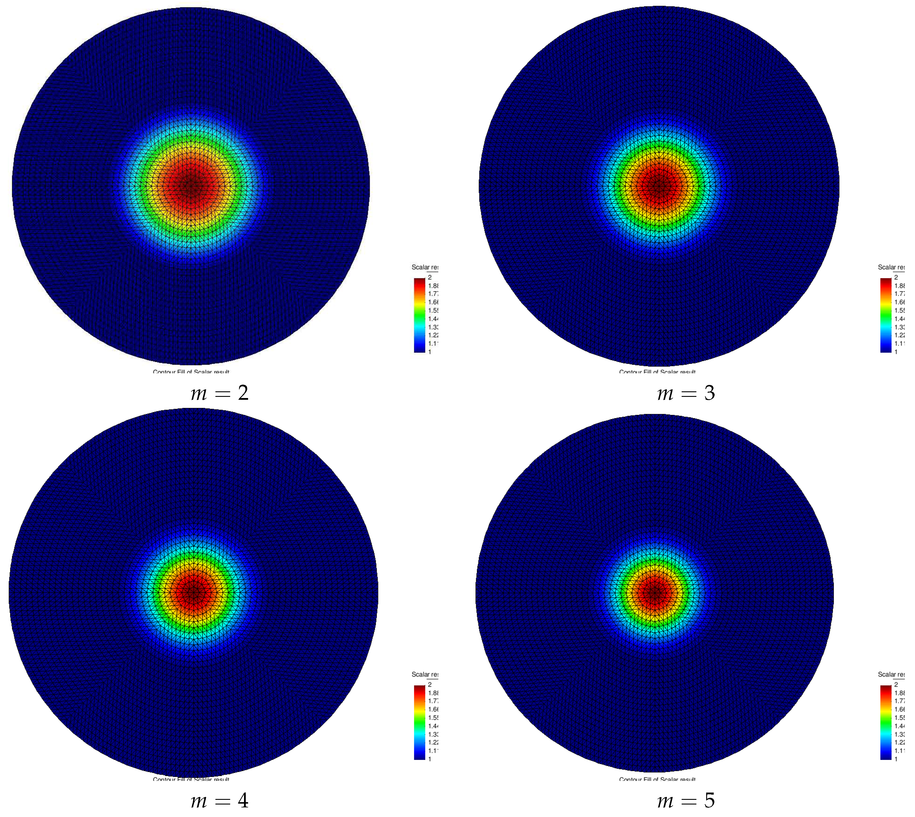
In our computations we used the software package Waves [34] for the finite element method applied to the solution of the model problem (2.2). The spatial domain $\Omega$ is discretized by a family of quasi-uniform meshes consisting of $2\times 2^{2l+2}$ triangles K for $l=1,...,6$, constructed as a certain mapping of the same number of triangles of the uniform mesh of the square $(-1,1)\times (-1,1)$, which is symmetric with respect to the cartesian axes and have their edges parallel to those axes and either to the line $x_1=x_2$ if $x_1{x}_2\ge 0$ or to the line $x_1=-x_2$ otherwise. The above mapping is defined by means of a suitable transformation of cartesian into polar coordinates. For each value of l we define a reference mesh size $h_l$ equal to $2^{-l}$.

We consider a partition of the time domain $(0,T)$ into time intervals $J=(t_{k-1},t_k]$ of equal length ${\tau }_l$ for a given number of time intervals $M,l=1,...,6$. We performed numerical tests taking $m=2,3,4,5$ in (5.130). We choose the time step ${\tau }_l=0.025\times 2^{-l},l=1,...,6$, which provides numerical stability for all meshes. We computed the maximum value over the time steps of the relative errors measured in the $L^2$-norms of the function, its gradient and its time-derivative in the polygon ${\Omega }_h$ for the different meshes in use. Now $\mathbf{e}$ and ${\mathbf{e}}_h$ being the exact and approximate solution of (2.2), setting $M:=T/{\tau }_l$, these quantities are represented by,

$$\begin{array}{cc}\hfill e_l^1& {\displaystyle =\frac{{\displaystyle \underset{1\le k\le M}{max}{\parallel {\mathbf{e}}^k-{\mathbf{e}}_h^k\parallel }_h}}{{\displaystyle \underset{1\le k\le M}{max}{\parallel {\mathbf{e}}^k\parallel }_h}},}\hfill \\ \hfill e_l^2& {\displaystyle =\frac{{\displaystyle \underset{1\le k\le M}{max}{\parallel \nabla ({\mathbf{e}}^k-{\mathbf{e}}_h^k)\parallel }_h}}{{\displaystyle \underset{1\le k\le M}{max}{\parallel \nabla {\mathbf{e}}^k\parallel }_h}},}\hfill \\ \hfill e_l^3& {\displaystyle =\frac{{\displaystyle \underset{1\le k\le M-1}{max}{\parallel {\left\{{\partial }_t(\mathbf{e}-{\mathbf{e}}_h)\right\}}^{k+1/2}\parallel }_h}}{{\displaystyle \underset{1\le k\le M-1}{max}{\parallel {\left\{{\partial }_t\mathbf{e}\right\}}^{k+1/2}\parallel }_h}}.}\hfill \end{array}$$

(5.131)

In Table 1, Table 2, Table 3 and Table 4 method’s convergence in these three senses is observed taking $m=2,3,4,5$ in (5.130). Figure 2 shows convergence rates of our numerical scheme based on a $P_1$ space discretization, taking the function $\epsilon$ defined by (5.130) with $m=2$ (on the left) and $m=3$ (on the right) for $\epsilon \left(r\right)$. Similar convergence results are presented in Figure 3 taking $m=4$ (on the left) and $m=5$ (on the right) in (5.130).

Table 1. Computed maximum relative errors $e_l$ in maximum energy, maximum $L^2$ and maximum in broken time error on different meshes with mesh sizes $h_l=2^{-l},l=1,...,6$ for the function $\epsilon$ with $m=2$ in (5.130).

l	$\mathit{n}\mathit{e}\mathit{l}$	$\mathit{n}\mathit{n}\mathit{o}$	${\mathit{e}}_{\mathit{l}}^{\left(1\right)}$	${\mathit{e}}_{\mathit{l}-1}^{\left(1\right)}/{\mathit{e}}_{\mathit{l}}^{\left(1\right)}$	${\mathit{e}}_{\mathit{l}}^{\left(2\right)}$	${\mathit{e}}_{\mathit{l}-1}^{\left(2\right)}/{\mathit{e}}_{\mathit{l}}^{\left(2\right)}$	${\mathit{e}}_{\mathit{l}}^{\left(3\right)}$	${\mathit{e}}_{\mathit{l}-1}^{\left(3\right)}/{\mathit{e}}_{\mathit{l}}^{\left(3\right)}$
1	32	25	0.6057		2.2827		3.1375
2	128	81	0.1499	4.0418	1.0769	2.1198	1.1536	2.7196
3	512	289	0.0333	4.5007	0.4454	2.4178	0.5776	1.9972
4	2048	1089	0.0078	4.2466	0.2077	2.1449	0.2802	2.0617
5	8192	4225	0.0019	4.1288	0.1066	1.9483	0.1379	2.0313
6	32768	16641	0.0005	4.0653	0.0535	1.9905	0.0690	1.9981

Table 1. Computed maximum relative errors $e_l$ in maximum energy, maximum $L^2$ and maximum in broken time error on different meshes with mesh sizes $h_l=2^{-l},l=1,...,6$ for the function $\epsilon$ with $m=2$ in (5.130).

l	$\mathit{n}\mathit{e}\mathit{l}$	$\mathit{n}\mathit{n}\mathit{o}$	${\mathit{e}}_{\mathit{l}}^{\left(1\right)}$	${\mathit{e}}_{\mathit{l}-1}^{\left(1\right)}/{\mathit{e}}_{\mathit{l}}^{\left(1\right)}$	${\mathit{e}}_{\mathit{l}}^{\left(2\right)}$	${\mathit{e}}_{\mathit{l}-1}^{\left(2\right)}/{\mathit{e}}_{\mathit{l}}^{\left(2\right)}$	${\mathit{e}}_{\mathit{l}}^{\left(3\right)}$	${\mathit{e}}_{\mathit{l}-1}^{\left(3\right)}/{\mathit{e}}_{\mathit{l}}^{\left(3\right)}$
1	32	25	0.6057		2.2827		3.1375
2	128	81	0.1499	4.0418	1.0769	2.1198	1.1536	2.7196
3	512	289	0.0333	4.5007	0.4454	2.4178	0.5776	1.9972
4	2048	1089	0.0078	4.2466	0.2077	2.1449	0.2802	2.0617
5	8192	4225	0.0019	4.1288	0.1066	1.9483	0.1379	2.0313
6	32768	16641	0.0005	4.0653	0.0535	1.9905	0.0690	1.9981

Table 2. Computed maximum relative errors $e_l$ in maximum energy, maximum $L^2$ and maximum in broken time error on different meshes with mesh sizes $h_l=2^{-l},l=1,...,6$ for the function $\epsilon$ with $m=3$ in (5.130).

l	$\mathit{n}\mathit{e}\mathit{l}$	$\mathit{n}\mathit{n}\mathit{o}$	${\mathit{e}}_{\mathit{l}}^{\left(1\right)}$	${\mathit{e}}_{\mathit{l}-1}^{\left(1\right)}/{\mathit{e}}_{\mathit{l}}^{\left(1\right)}$	${\mathit{e}}_{\mathit{l}}^{\left(2\right)}$	${\mathit{e}}_{\mathit{l}-1}^{\left(2\right)}/{\mathit{e}}_{\mathit{l}}^{\left(2\right)}$	${\mathit{e}}_{\mathit{l}}^{\left(3\right)}$	${\mathit{e}}_{\mathit{l}-1}^{\left(3\right)}/{\mathit{e}}_{\mathit{l}}^{\left(3\right)}$
1	32	25	0.6144		1.8851		3.0462
2	128	81	0.1511	4.0666	1.0794	1.7464	1.1417	2.6682
3	512	289	0.0339	4.4553	0.4713	2.2904	0.5680	2.0099
4	2048	1089	0.0080	4.2216	0.2166	2.1753	0.2760	2.0583
5	8192	4225	0.0019	4.1207	0.1137	1.9049	0.1354	2.0381
6	32768	16641	0.0005	4.0615	0.0566	2.0092	0.0677	1.9997

Table 2. Computed maximum relative errors $e_l$ in maximum energy, maximum $L^2$ and maximum in broken time error on different meshes with mesh sizes $h_l=2^{-l},l=1,...,6$ for the function $\epsilon$ with $m=3$ in (5.130).

l	$\mathit{n}\mathit{e}\mathit{l}$	$\mathit{n}\mathit{n}\mathit{o}$	${\mathit{e}}_{\mathit{l}}^{\left(1\right)}$	${\mathit{e}}_{\mathit{l}-1}^{\left(1\right)}/{\mathit{e}}_{\mathit{l}}^{\left(1\right)}$	${\mathit{e}}_{\mathit{l}}^{\left(2\right)}$	${\mathit{e}}_{\mathit{l}-1}^{\left(2\right)}/{\mathit{e}}_{\mathit{l}}^{\left(2\right)}$	${\mathit{e}}_{\mathit{l}}^{\left(3\right)}$	${\mathit{e}}_{\mathit{l}-1}^{\left(3\right)}/{\mathit{e}}_{\mathit{l}}^{\left(3\right)}$
1	32	25	0.6144		1.8851		3.0462
2	128	81	0.1511	4.0666	1.0794	1.7464	1.1417	2.6682
3	512	289	0.0339	4.4553	0.4713	2.2904	0.5680	2.0099
4	2048	1089	0.0080	4.2216	0.2166	2.1753	0.2760	2.0583
5	8192	4225	0.0019	4.1207	0.1137	1.9049	0.1354	2.0381
6	32768	16641	0.0005	4.0615	0.0566	2.0092	0.0677	1.9997

Table 3. Computed maximum relative errors $e_l$ in maximum energy, maximum $L^2$ and maximum in broken time error on different meshes with mesh sizes $h_l=2^{-l},l=1,...,6$ for the function $\epsilon$ with $m=4$ in (5.130).

l	$\mathit{n}\mathit{e}\mathit{l}$	$\mathit{n}\mathit{n}\mathit{o}$	${\mathit{e}}_{\mathit{l}}^{\left(1\right)}$	${\mathit{e}}_{\mathit{l}-1}^{\left(1\right)}/{\mathit{e}}_{\mathit{l}}^{\left(1\right)}$	${\mathit{e}}_{\mathit{l}}^{\left(2\right)}$	${\mathit{e}}_{\mathit{l}-1}^{\left(2\right)}/{\mathit{e}}_{\mathit{l}}^{\left(2\right)}$	${\mathit{e}}_{\mathit{l}}^{\left(3\right)}$	${\mathit{e}}_{\mathit{l}-1}^{\left(3\right)}/{\mathit{e}}_{\mathit{l}}^{\left(3\right)}$
1	32	25	0.6122		1.9517		3.0545
2	128	81	0.1529	4.0027	1.0896	1.7912	1.1445	2.6689
3	512	289	0.0346	4.4266	0.4879	2.2331	0.5639	2.0296
4	2048	1089	0.0082	4.2069	0.2234	2.1839	0.2728	2.0667
5	8192	4225	0.0020	4.1151	0.1183	1.8879	0.1336	2.0418
6	32768	16641	0.0005	4.0585	0.0595	1.9890	0.0668	2.0008

Table 3. Computed maximum relative errors $e_l$ in maximum energy, maximum $L^2$ and maximum in broken time error on different meshes with mesh sizes $h_l=2^{-l},l=1,...,6$ for the function $\epsilon$ with $m=4$ in (5.130).

l	$\mathit{n}\mathit{e}\mathit{l}$	$\mathit{n}\mathit{n}\mathit{o}$	${\mathit{e}}_{\mathit{l}}^{\left(1\right)}$	${\mathit{e}}_{\mathit{l}-1}^{\left(1\right)}/{\mathit{e}}_{\mathit{l}}^{\left(1\right)}$	${\mathit{e}}_{\mathit{l}}^{\left(2\right)}$	${\mathit{e}}_{\mathit{l}-1}^{\left(2\right)}/{\mathit{e}}_{\mathit{l}}^{\left(2\right)}$	${\mathit{e}}_{\mathit{l}}^{\left(3\right)}$	${\mathit{e}}_{\mathit{l}-1}^{\left(3\right)}/{\mathit{e}}_{\mathit{l}}^{\left(3\right)}$
1	32	25	0.6122		1.9517		3.0545
2	128	81	0.1529	4.0027	1.0896	1.7912	1.1445	2.6689
3	512	289	0.0346	4.4266	0.4879	2.2331	0.5639	2.0296
4	2048	1089	0.0082	4.2069	0.2234	2.1839	0.2728	2.0667
5	8192	4225	0.0020	4.1151	0.1183	1.8879	0.1336	2.0418
6	32768	16641	0.0005	4.0585	0.0595	1.9890	0.0668	2.0008

Table 4. Computed maximum relative errors $e_l$ in maximum energy, maximum $L^2$ and maximum in broken time error on different meshes with mesh sizes $h_l=2^{-l},l=1,...,6$ for the function $\epsilon$ with $m=5$ in (5.130).

l	$\mathit{n}\mathit{e}\mathit{l}$	$\mathit{n}\mathit{n}\mathit{o}$	${\mathit{e}}_{\mathit{l}}^{\left(1\right)}$	${\mathit{e}}_{\mathit{l}-1}^{\left(1\right)}/{\mathit{e}}_{\mathit{l}}^{\left(1\right)}$	${\mathit{e}}_{\mathit{l}}^{\left(2\right)}$	${\mathit{e}}_{\mathit{l}-1}^{\left(2\right)}/{\mathit{e}}_{\mathit{l}}^{\left(2\right)}$	${\mathit{e}}_{\mathit{l}}^{\left(3\right)}$	${\mathit{e}}_{\mathit{l}-1}^{\left(3\right)}/{\mathit{e}}_{\mathit{l}}^{\left(3\right)}$
1	32	25	0.6107		1.9930		3.0603
2	128	81	0.1546	3.9505	1.1006	1.8108	1.1464	2.6696
3	512	289	0.0351	4.4031	0.4982	2.2090	0.5619	2.0403
4	2048	1089	0.0084	4.1954	0.2288	2.1777	0.2706	2.0765
5	8192	4225	0.0020	4.1106	0.1223	1.8715	0.1325	2.0417
6	32768	16641	0.0005	4.0561	0.0607	2.0139	0.0662	2.0011

Table 4. Computed maximum relative errors $e_l$ in maximum energy, maximum $L^2$ and maximum in broken time error on different meshes with mesh sizes $h_l=2^{-l},l=1,...,6$ for the function $\epsilon$ with $m=5$ in (5.130).

l	$\mathit{n}\mathit{e}\mathit{l}$	$\mathit{n}\mathit{n}\mathit{o}$	${\mathit{e}}_{\mathit{l}}^{\left(1\right)}$	${\mathit{e}}_{\mathit{l}-1}^{\left(1\right)}/{\mathit{e}}_{\mathit{l}}^{\left(1\right)}$	${\mathit{e}}_{\mathit{l}}^{\left(2\right)}$	${\mathit{e}}_{\mathit{l}-1}^{\left(2\right)}/{\mathit{e}}_{\mathit{l}}^{\left(2\right)}$	${\mathit{e}}_{\mathit{l}}^{\left(3\right)}$	${\mathit{e}}_{\mathit{l}-1}^{\left(3\right)}/{\mathit{e}}_{\mathit{l}}^{\left(3\right)}$
1	32	25	0.6107		1.9930		3.0603
2	128	81	0.1546	3.9505	1.1006	1.8108	1.1464	2.6696
3	512	289	0.0351	4.4031	0.4982	2.2090	0.5619	2.0403
4	2048	1089	0.0084	4.1954	0.2288	2.1777	0.2706	2.0765
5	8192	4225	0.0020	4.1106	0.1223	1.8715	0.1325	2.0417
6	32768	16641	0.0005	4.0561	0.0607	2.0139	0.0662	2.0011

Figure 2. Maximum in time of relative errors for $m=2$ (left) and $m=3$ (right)

Figure 2. Maximum in time of relative errors for $m=2$ (left) and $m=3$ (right)

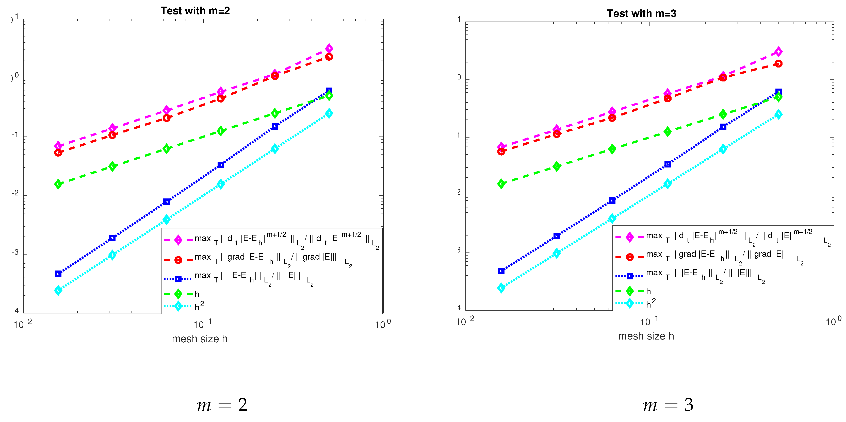
Figure 3. Maximum in time of relative errors for $m=4$ (left) and $m=5$ (right)

Figure 3. Maximum in time of relative errors for $m=4$ (left) and $m=5$ (right)

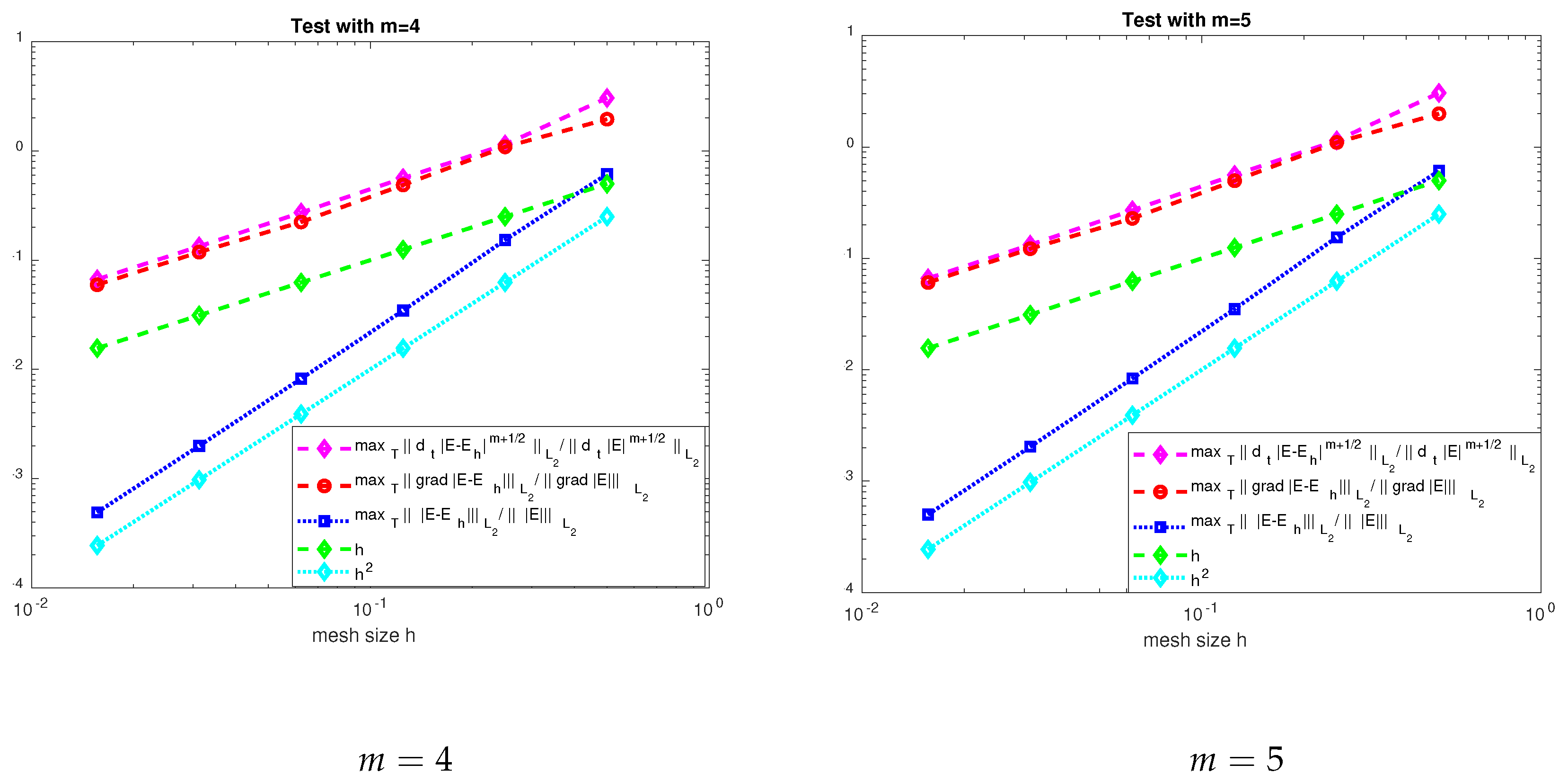
Observation of these tables and figures clearly indicates that our scheme behaves like a first order method in the (semi-)norm of $L^{\infty }[(0,T);H^1(\Omega )]$ for $\mathbf{e}$ and in the norm of $L^{\infty }[(0,T);L^2(\Omega )]$ for ${\partial }_t\mathbf{e}$ for all the chosen values of m. As far as the values of m greater or equal to 4 are concerned this perfectly conforms to the a priori error estimates given in Section 4. However, those tables and figures also show that such theoretical predictions extend to cases not considered in our analysis such as $m=2$ and $m=3$, in which the regularity of the exact solution is lower than assumed. Otherwise stated, some of our assumptions seem to be of academic interest only and a lower regularity of the solution such as $H^2(\Omega \times (0,T))$ should be sufficient to attain optimal first order convergence in both senses. On the other hand second-order convergence can be expected from our scheme in the norm of $L^{\infty }[(0,T);L^2(\Omega )]$ for $\mathbf{e}$, according to Table 1, Table 2, Table 3 and Table 4 and Figure 2 and Figure 3.

6. Final remarks

As previously noted, the approach advocated in this work was extensively and successfully tested in the framework of the solution of CIPs governed by Maxwell’s equations. More specifically it was used with minor modifications to solve both the direct problem and the adjoint problem, as steps of an adaptive algorithm to determine the unknown dielectric permittivity. More details on this procedure can be found in [9] and references therein.

As a matter of fact, the method studied in this paper was designed to handle composite dielectrics structured in such a way that layers with higher permittivity are completely surrounded by layers with a (constant) lower permittivity, say $\epsilon =1$. It should be noted, however, that the assumption that $\epsilon$ attains a minimum in the outer layer was made here only to simplify things. Actually, under the same assumptions (4.129) also applies to the case where $\epsilon$ in inner layers is allowed to be smaller than in the outer layer, say $\epsilon <1$. We refer to [6] for further details.

Another issue that is worth a comment is the practical calculation of the term $(\nabla ·\epsilon {\mathbf{e}}_h^k,\nabla ·\mathbf{v})$ in (3.14). Unless $\epsilon$ is a simple function such as a polynomial, it is not possible to compute this term exactly. That is why we recommend the use of the trapezoidal rule to carry out these computations. At the price of small adjustments in some terms involving norms of $\epsilon$, the thus modified scheme is stable in the same sense as (4.54). Moreover, the qualitative convergence result (4.129) remains unchanged, provided a little more regularity is required from $\epsilon$. We skip details for the sake of brevity.

References

- R.A. Adams, Sobolev Spaces, Academic Press, N.Y., 1975.
- F. Assous, P. Degond, E. Heintze, P.-A. Raviart, On a finite-element method for solving the three-dimensional Maxwell equations, J. Computational Physics, 109 (1993), 222–237. [CrossRef]
- S. Badia, R. Codina, A Nodal-based Finite Element Approximation of the Maxwell Problem Suitable for Singular Solutions, SIAM J. Numer. Anal., 50-2 (2012), 398–417. [CrossRef]
- L. Beilina, M. Grote, Adaptive Hybrid Finite Element/Difference Method for Maxwell’s equations, TWMS J. of Pure and Applied Mathematics, 1-2 (2010), 176-197. [CrossRef]
- L. Beilina, Energy estimates and numerical verification of the stabilized Domain Decomposition Finite Element/Finite Difference approach for time-dependent Maxwell’s system, Cent. Eur. J. Math., 11-4 (2013) 702-733. [CrossRef]
- L. Beilina, V. Ruas, An explicit P1 finite element scheme for Maxwell’s equations with constant permittivity in a boundary neighborhood, arXiv:1808.10720, 2020.
- L. Beilina, V. Ruas, Convergence of Explicit P1 Finite-Element Solutions to Maxwell’s Equations, Springer Proceedings in Mathematics and Statistics, vol 328, p.91-103, Springer, 2020.
- L. Beilina, V. Ruas, On the Maxwell-wave equation coupling problem and its explicit finite-element solution, Applications of Mathematics, open access (2022). [CrossRef]
- J. Bondestam-Malmberg, L. Beilina, An adaptive finite element method in quantitative reconstruction of small inclusions from limited observations, Appl. Maths & Information Sci., 12-1 (2018), 1–19.
- A. Bossavit, Computational Electromagnetism, Variational Formulations, Complementary, Edge Elements, in: Electromagnetism, vol. 2, Academic Press, New York, 1998.
- F. Brezzi, On the existence, uniqueness and approximation of saddle-point problems arising from Lagrange multipliers, RAIRO Analyse Numérique, 8-2 (1974), 129-151.
- J.H. Carneiro de Araujo, P.D. Gomes, V. Ruas, Study of a finite element method for the time-dependent generalized Stokes system associated with viscoelastic flow, J. Computational Applied Mathematics, 234-8 (2010), 2562-2577. [CrossRef]
- V.C. Chen and W.V. Wahl, Das Rand-Anfangswertproblem für quasilineare Wellen-gleichungen in Sobolevräumen niedriger Ordnung, Z. reine angew. Math., 337 (1982), 77-112. [CrossRef]
- P.G. Ciarlet, The Finite Element Method for Elliptic Problems, North Holland, 1978.
- P. Ciarlet Jr, J. Zou, Fully discrete finite element approaches for time-dependent Maxwell’s equations, Numerische Mathematik, 82-2 (1999), 193–219. [CrossRef]
- P. Ciarlet Jr, Augmented formulations for solving Maxwell equations, Computer Methods in Applied Mechanics and Engineering, 194-2–5 (2005), 559–586. [CrossRef]
- P. Ciarlet Jr, E. Jamelot, Continuous Galerkin methods for solving the time-dependent Maxwell equations in 3D geometries, J. Computational Physics, 226-1 (2007), 1122-1135. [CrossRef]
- G. Cohen, P. Monk, Gauss point mass lumping schemes for Maxwell’s equations, Numerical Methods for Partial Differential Equations, 14-1 (1998), 63–88.
- M. Costabel, A coercive bilinear form for Maxwell’s equations, J. Math. Anal. Appl., 157-2 (1991), 527–541. [CrossRef]
- M. Costabel, M. Dauge, Singularities of Maxwell’s equations on polyhedral domains, Analysis, Numerics and Applications of Differential and Integral Equations, Pitman Research Notes in Mathematics Series, Vol. 379, p.69–76, 1998.
- M. Costabel, M. Dauge, Weighted regularization of Maxwell’s equations in polyhedral domains. A rehabilitation of nodal finite elements, Numerische Mathematik, 93-2 (2002), 239–277. [CrossRef]
- A. Ditkowski and D. Gottlieb, On the Engquist–Majda absorbing boundary conditions for hyperbolic systems, Contemporary Mathematics, 330 (2003), 55–72.
- A. Elmkies and P. Joly, Finite elements and mass lumping for Maxwell’s equations: the 2D case. Numerical Analysis, C. R. Acad.Sci.Paris, 324, pp. 1287–1293, 1997.
- B. Engquist, A. Majda, Absorbing boundary conditions for the numerical simulation of waves, Mathematics of Computation, 31 (1977), 629-651.
- V. Girault, P.A. Raviart, Finite Element Methods for Navier-Stokes Equations, Springer Series in Computational Mathematics, Vol. 5, Springer-Verlag, Berlin, 1986.
- P. Grisvard, Sigularities in Boundary Value Problems, Masson, Paris, 1992.
- E. Jamelot, Résolution des équations de Maxwell avec des éléments finis de Galerkin continus, thèse doctorale, École Polytechnique, Palaiseau, France, 2005.
- P. Monk. Finite Element Methods for Maxwell’s Equations, Clarendon Press, 2003.
- J.-C. Nédélec, Mixed finite elements in R3, Numerische Mathematik, 35 (1980), 315-341. [CrossRef]
- P.-A. Raviart and J.-M. Thomas, Mixed Finite Element Methods for Second Order Elliptic Problems, Lecture Notes in Mathematics, Springer Verlag, 606: 292-315, 1977.
- V. Ruas, Numerical Methods for Partial Differential Equations; an Introduction, Wiley, 2016.
- V. Ruas and M.A. Silva Ramos, A Hermite Method for Maxwell’s Equations, Appl. Maths & Information Sci., 12-2 (2018), 271–283. [CrossRef]
- V. Thomée, Galerkin Finite Element Methods for Parabolic Problems, Springer Series in Computational Mathematics, Second edition, 1997.
- WavES, the software package, http://www.waves24.com.
Disclaimer/Publisher’s Note: The statements, opinions and data contained in all publications are solely those of the individual author(s) and contributor(s) and not of MDPI and/or the editor(s). MDPI and/or the editor(s) disclaim responsibility for any injury to people or property resulting from any ideas, methods, instructions or products referred to in the content. |
© 2024 by the authors. Licensee MDPI, Basel, Switzerland. This article is an open access article distributed under the terms and conditions of the Creative Commons Attribution (CC BY) license (http://creativecommons.org/licenses/by/4.0/).
Copyright: This open access article is published under a Creative Commons CC BY 4.0 license, which permit the free download, distribution, and reuse, provided that the author and preprint are cited in any reuse.